
Numerical Study of the Hygrothermal Effects on Low Velocity Impact Induced Indentation and Its Rebound in Composite Laminate


Abstract
:1. Introduction
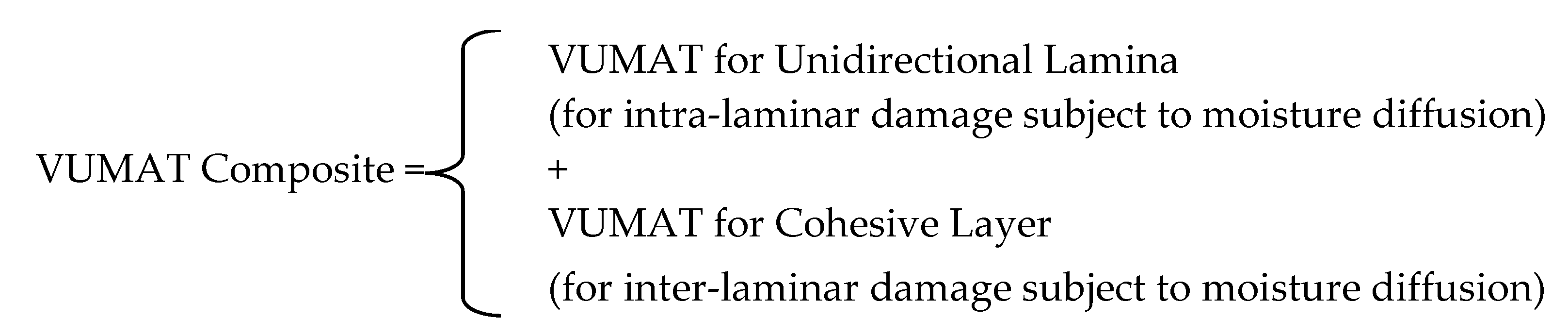
2. Moisture-Dependent Viscoelastic Constitution for Composite Laminate
2.1. Constitutive Equations for a UD Laminae Ply
2.2. Failure Law of UD Laminae Ply
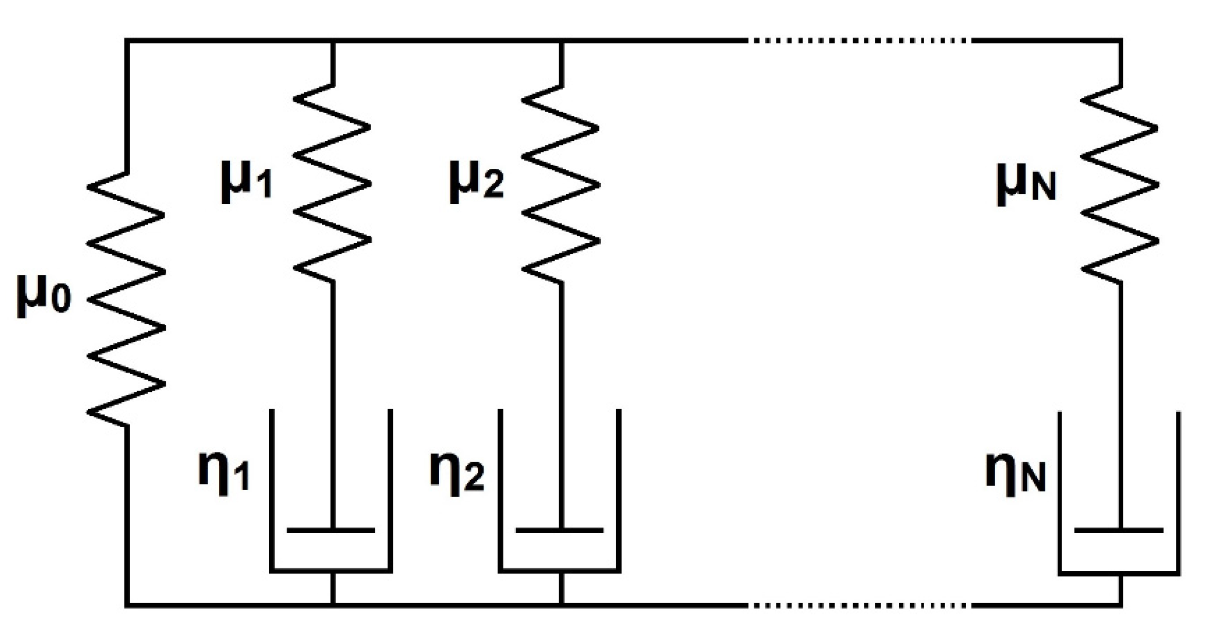
2.3. Constitutive Equations for the Cohesive Interface
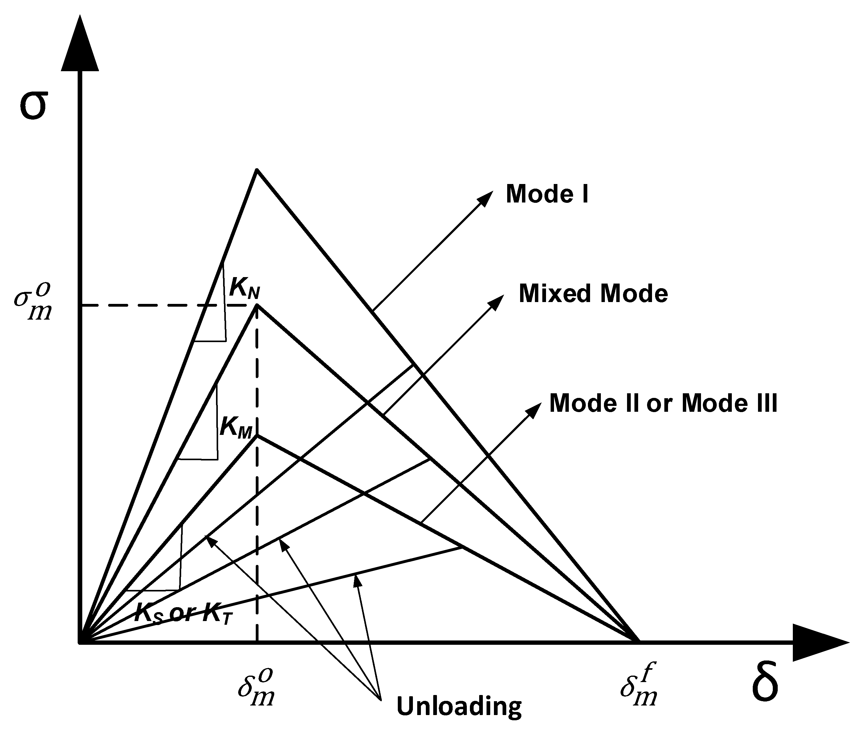
2.4. Damage Law of Cohesive Interface
3. Experiment and FEM Simulation
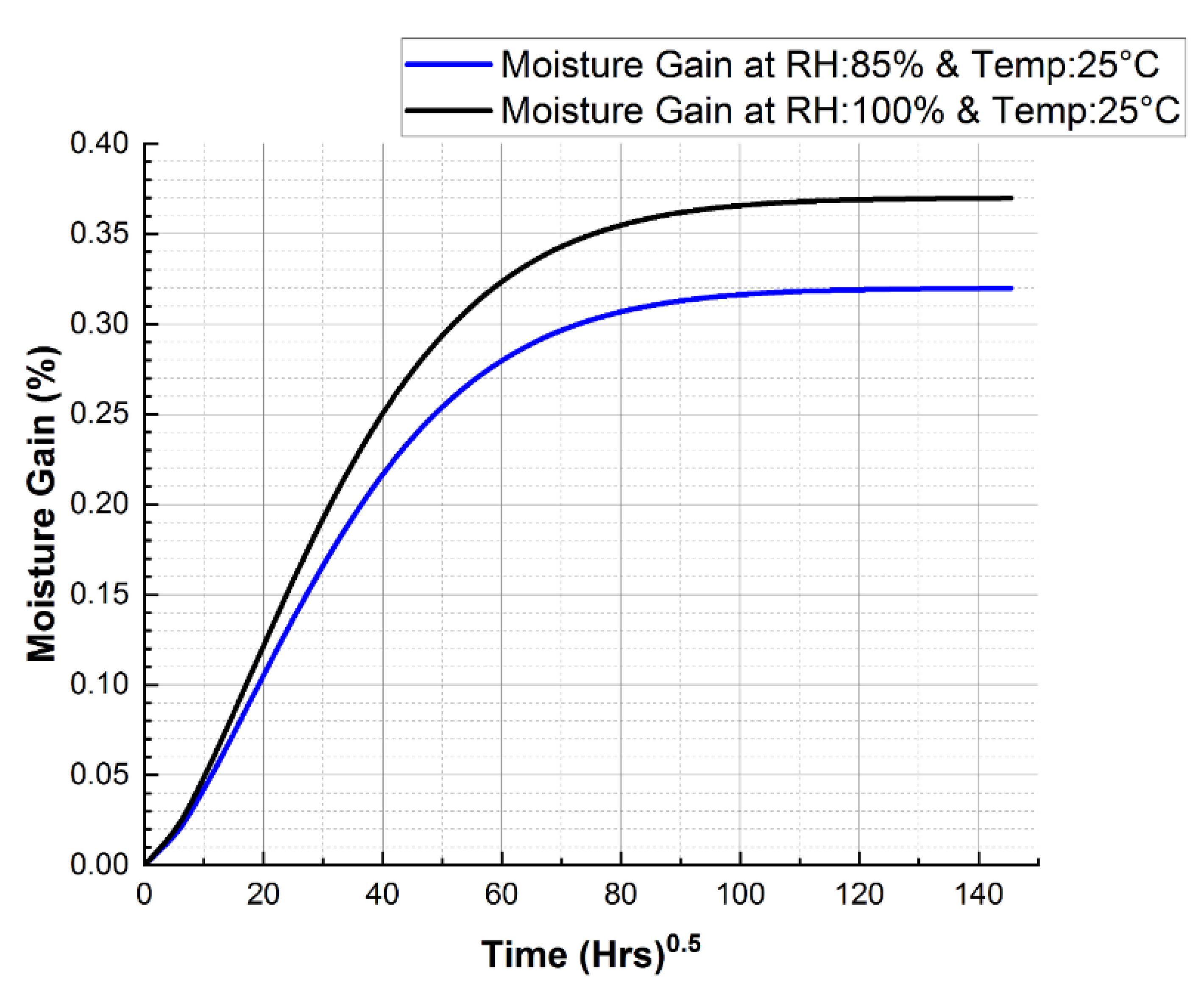
3.1. Experimental Methodology
- I.
- 25 °C/RH: 85%;
- II.
- 25 °C/RH: 100%.
3.2. Simulation Methodology
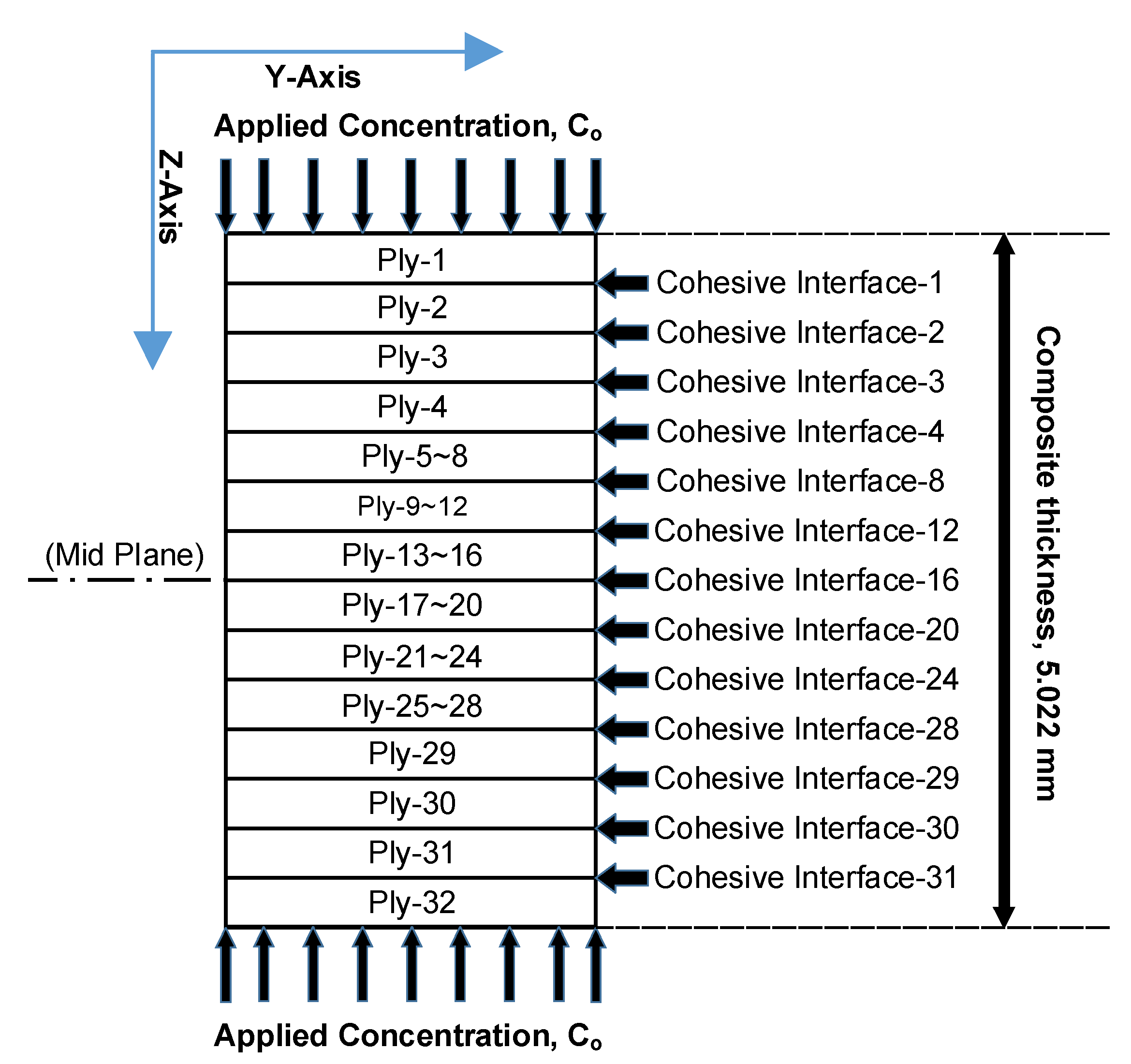
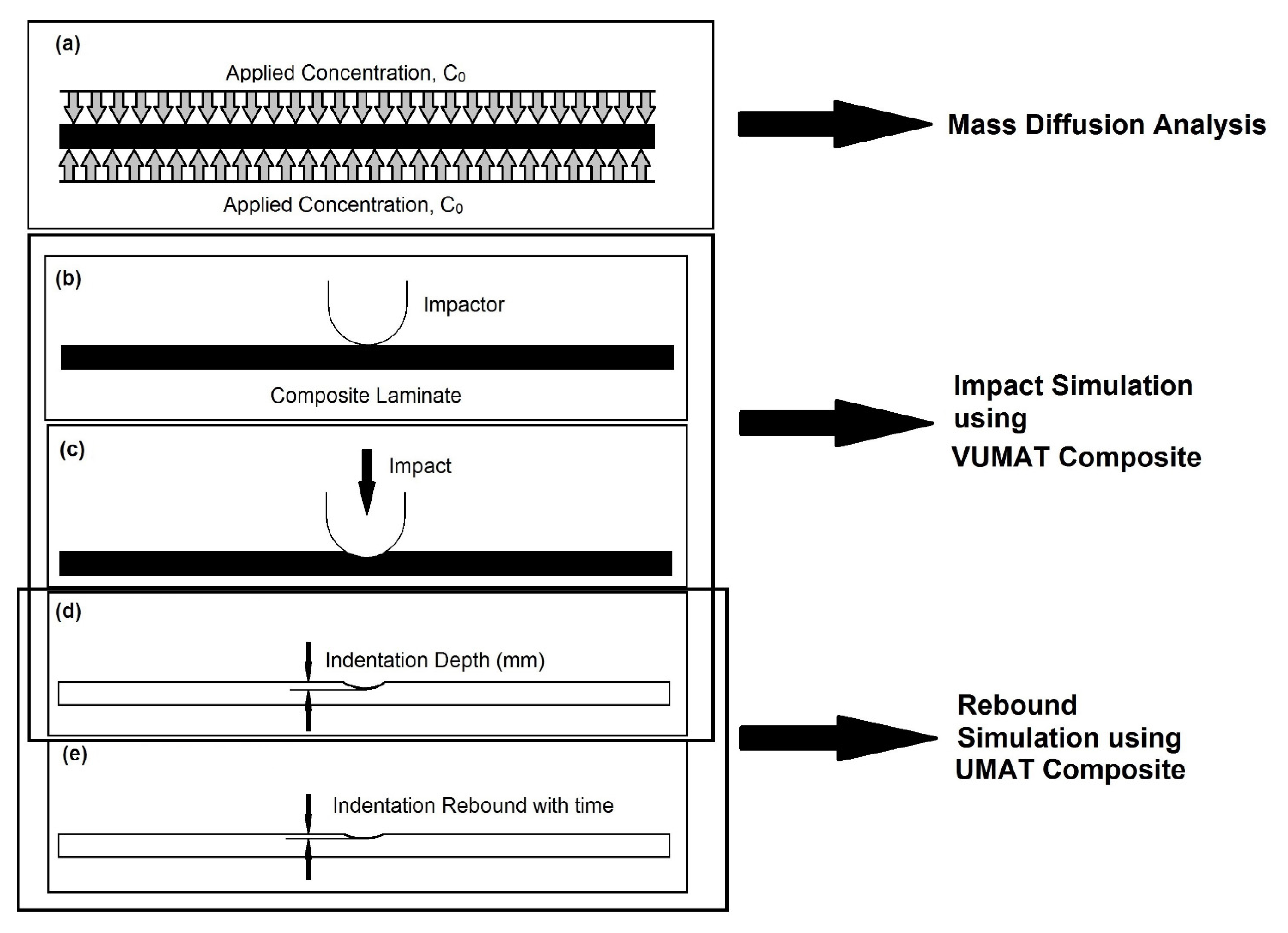
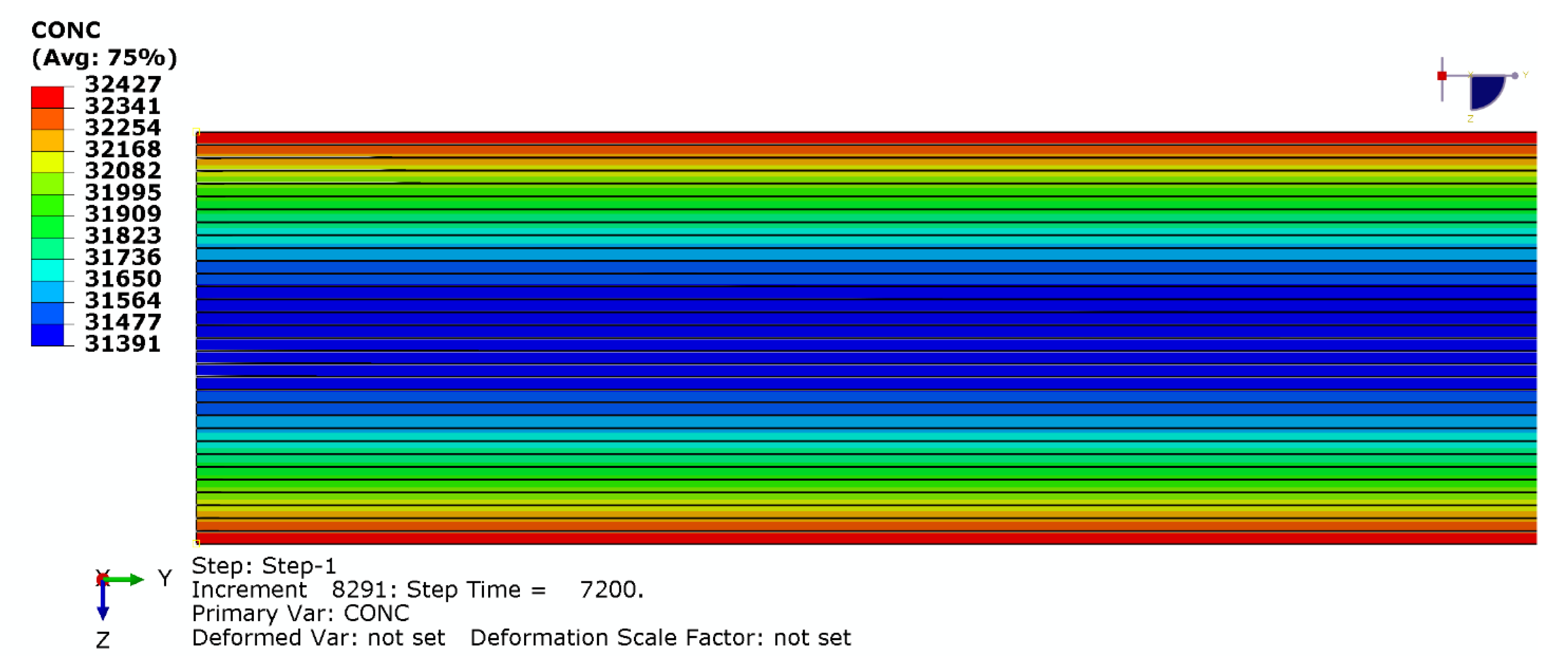
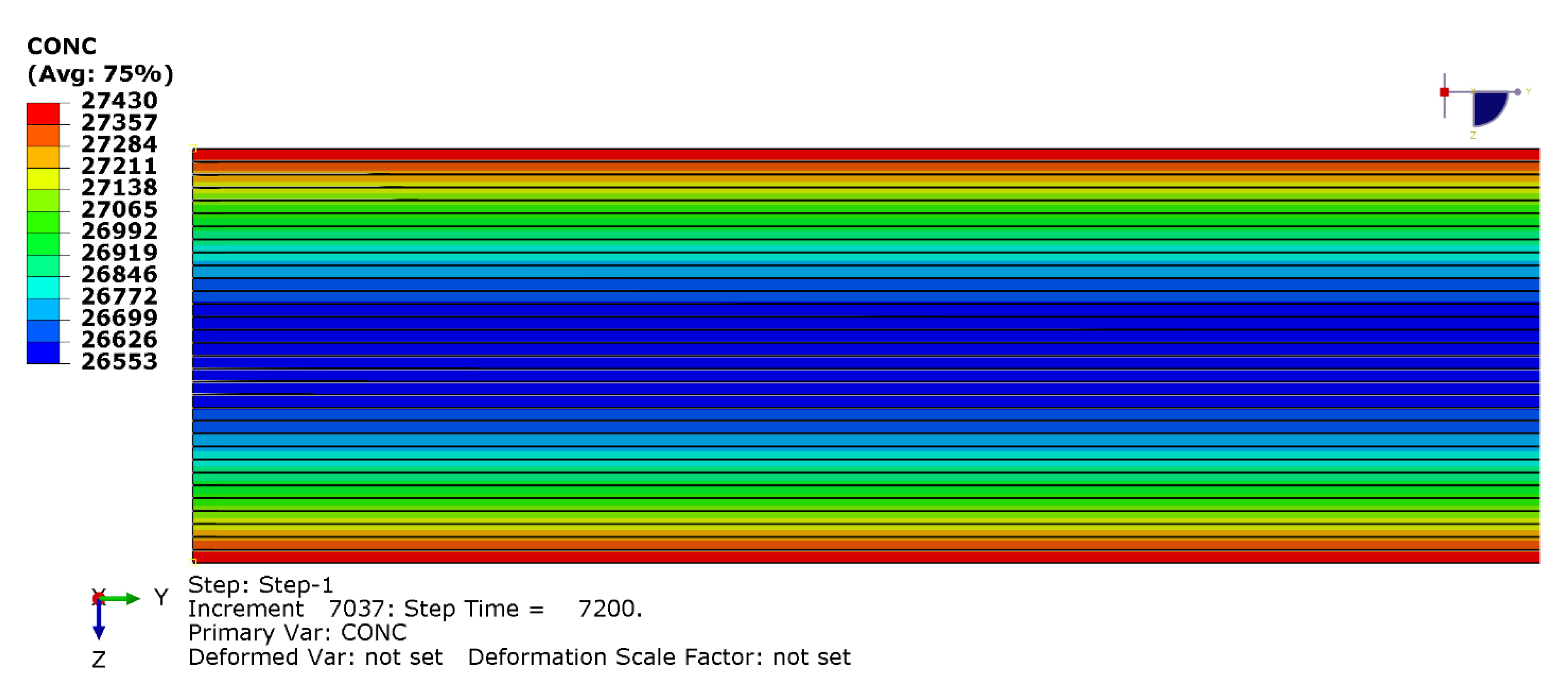
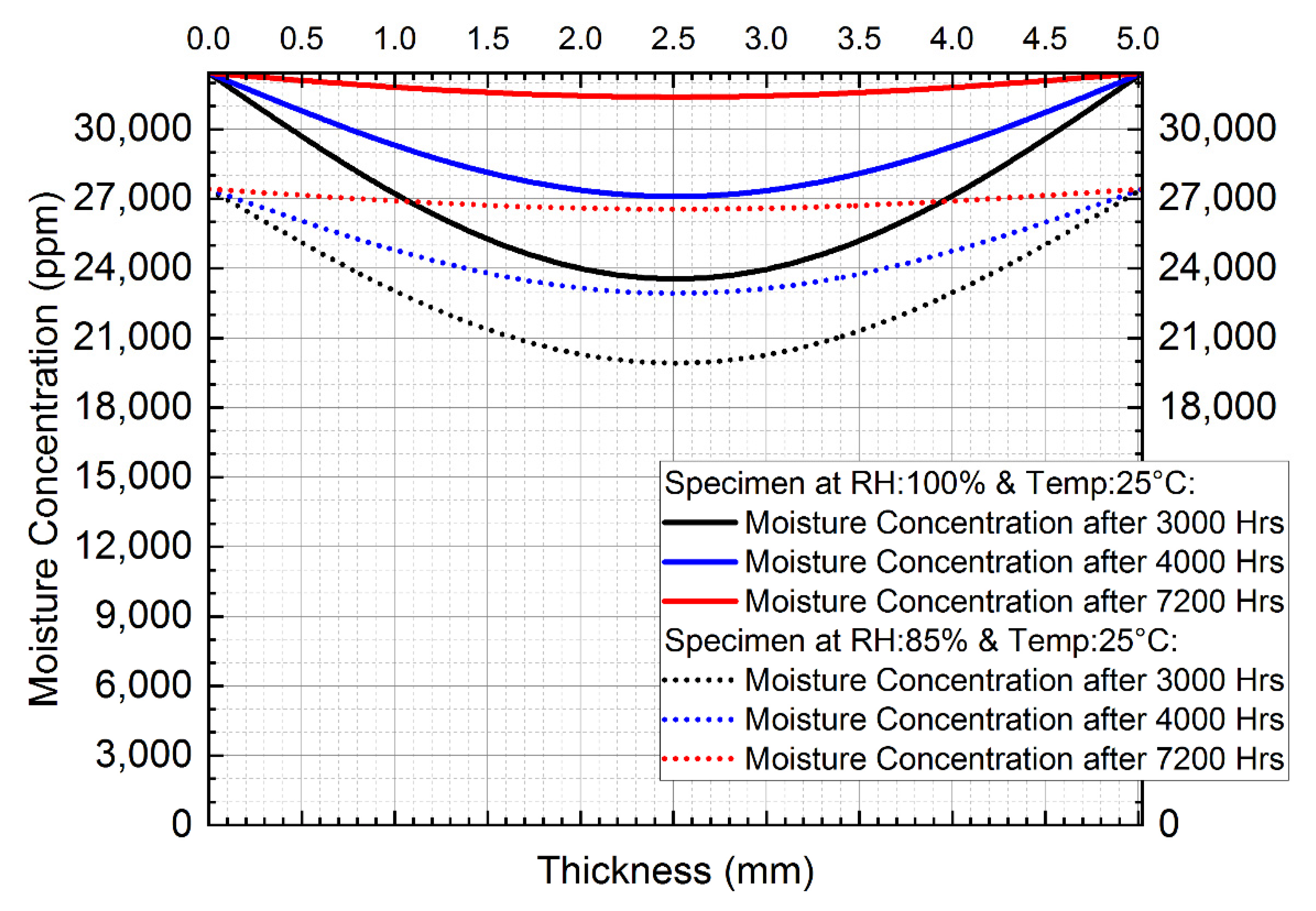
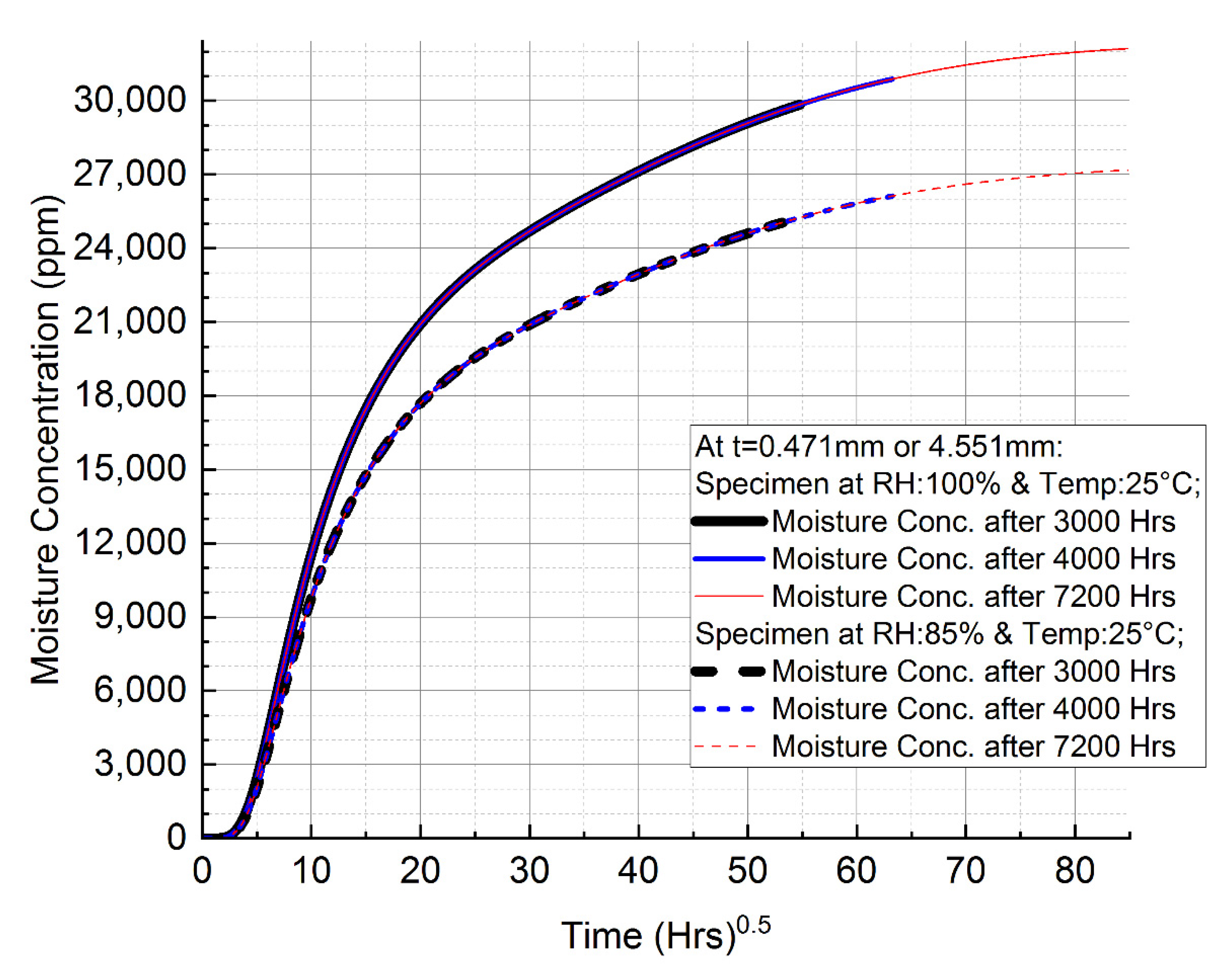
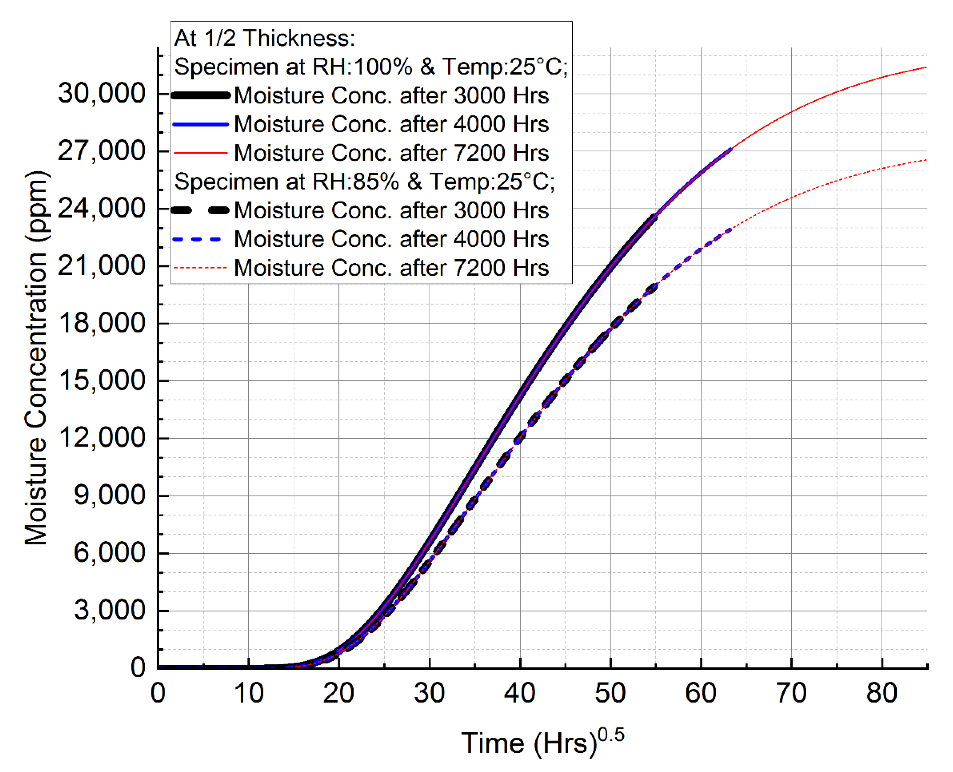
3.2.1. Simulation for the Moisture Diffusion Case
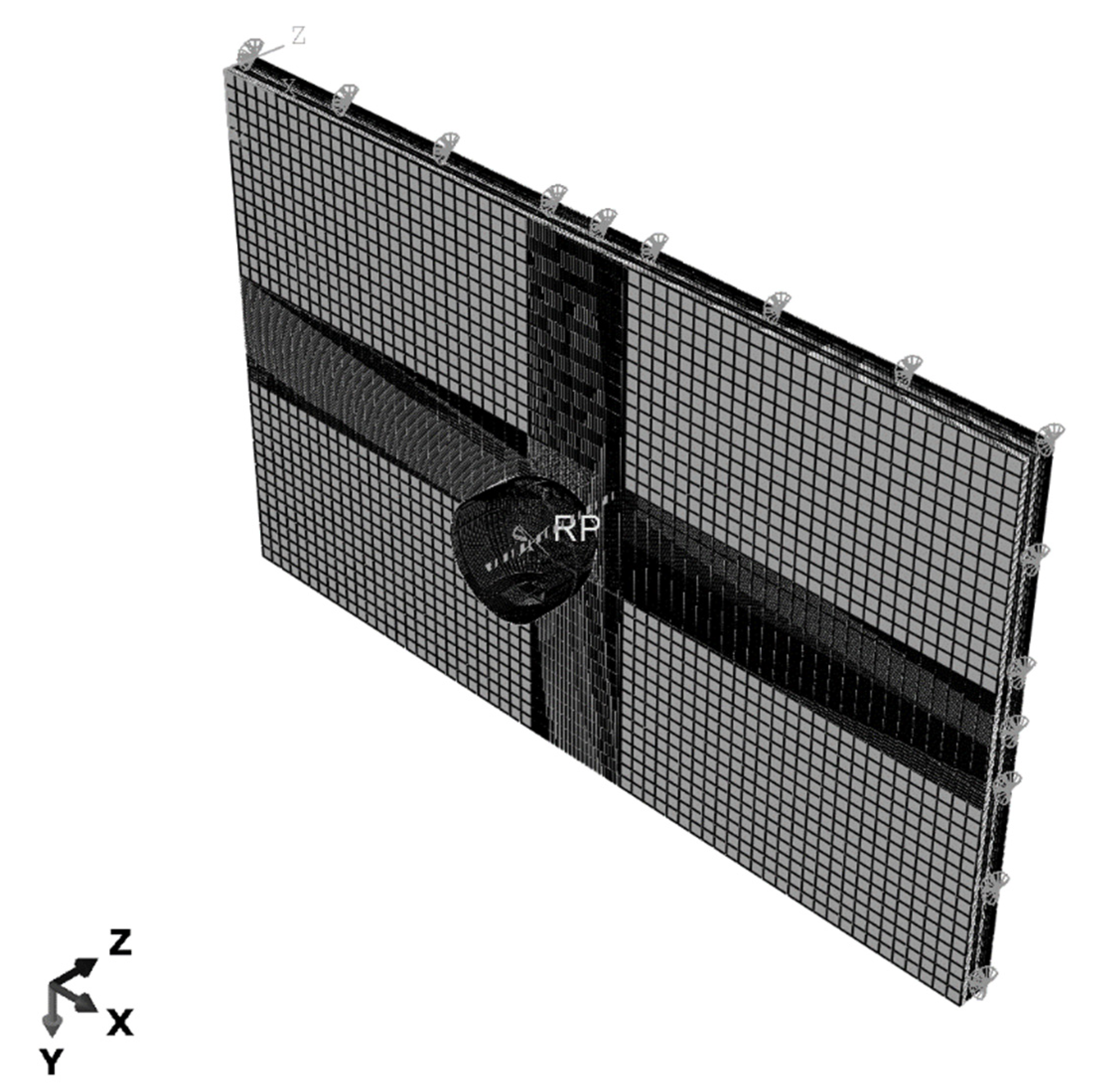
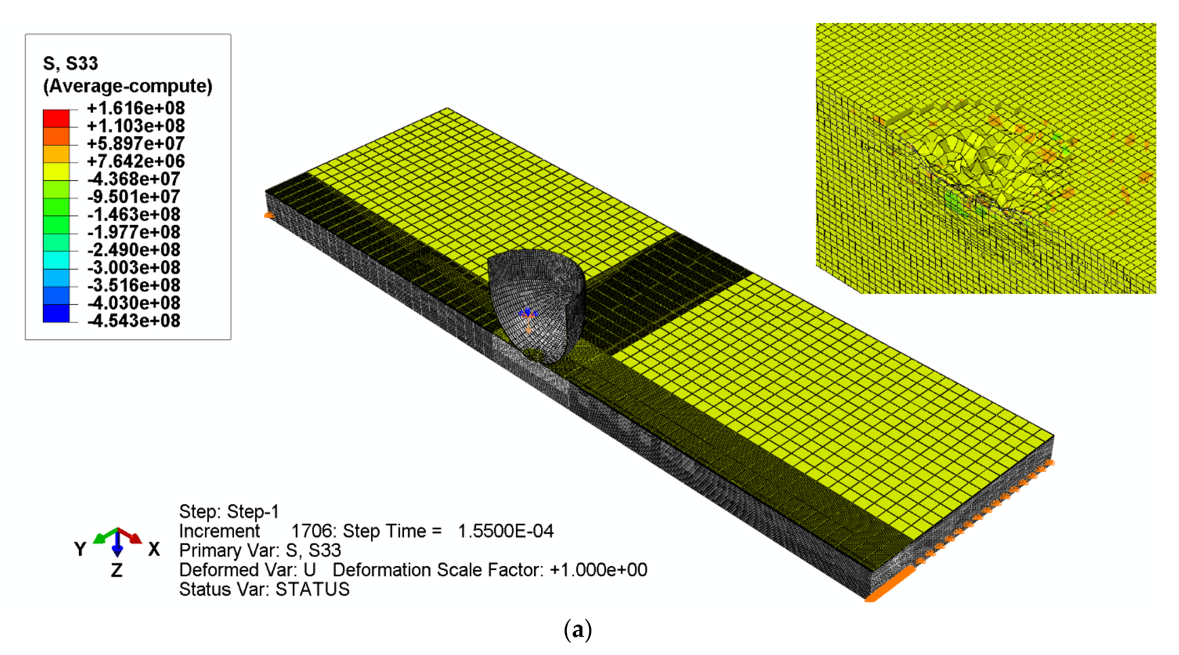
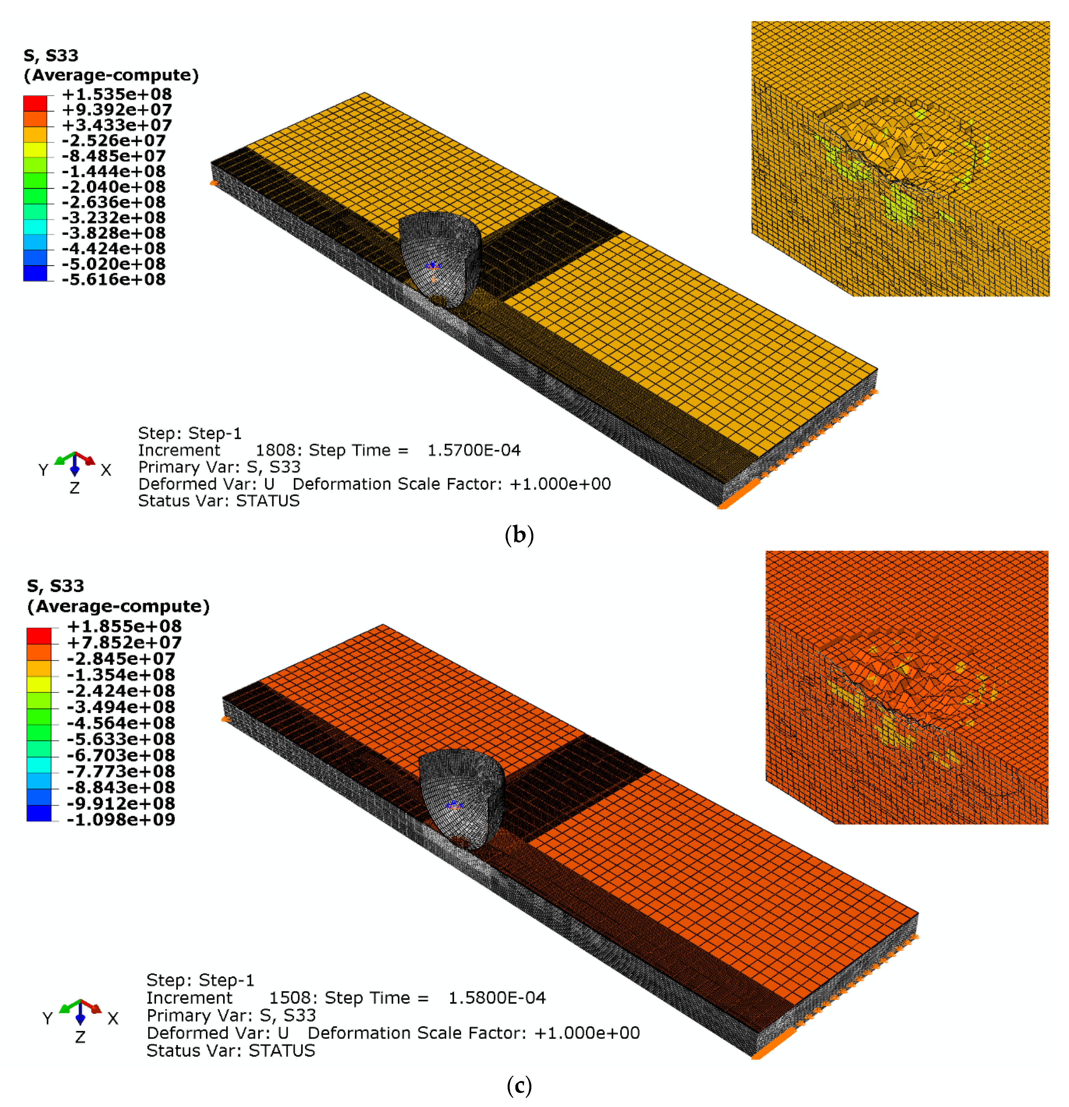
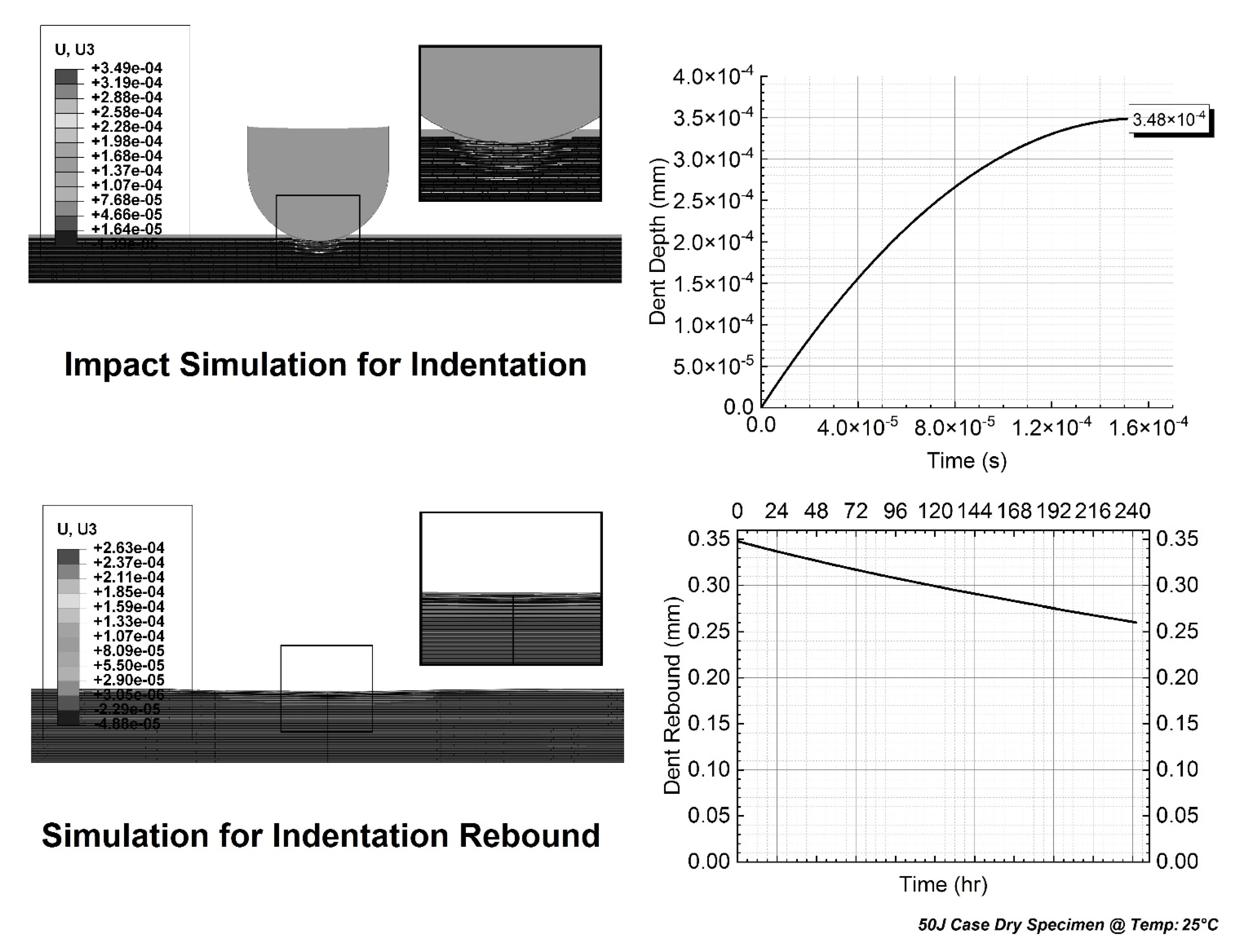
3.2.2. Simulation for the Impact Case

3.2.3. Simulation for the Rebound Case

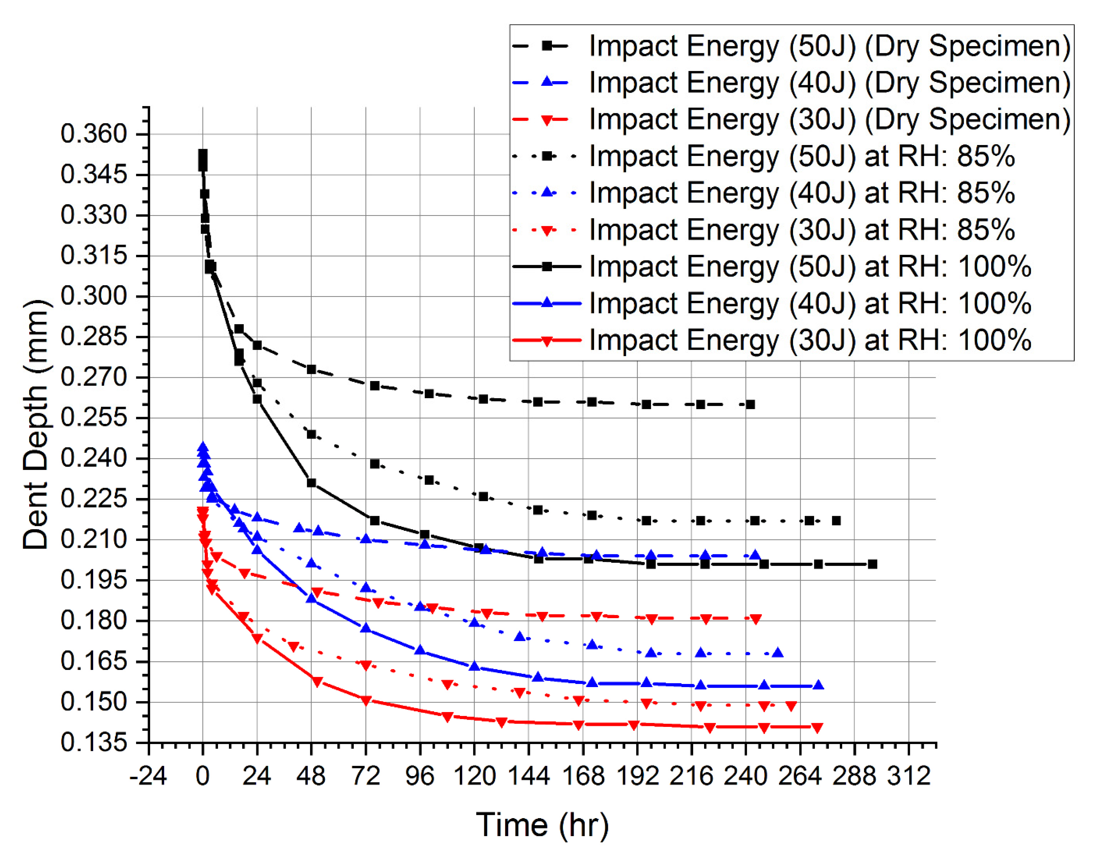
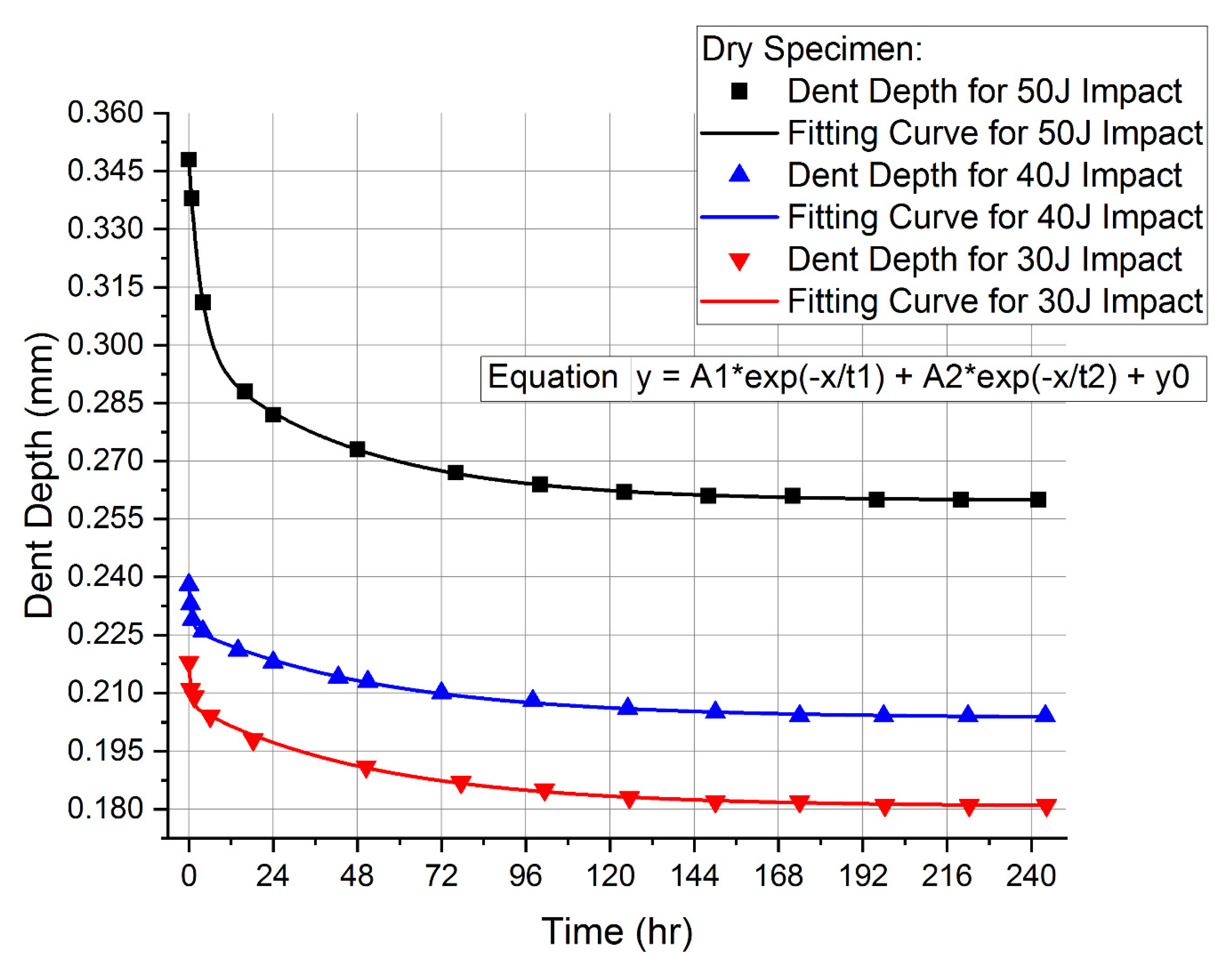
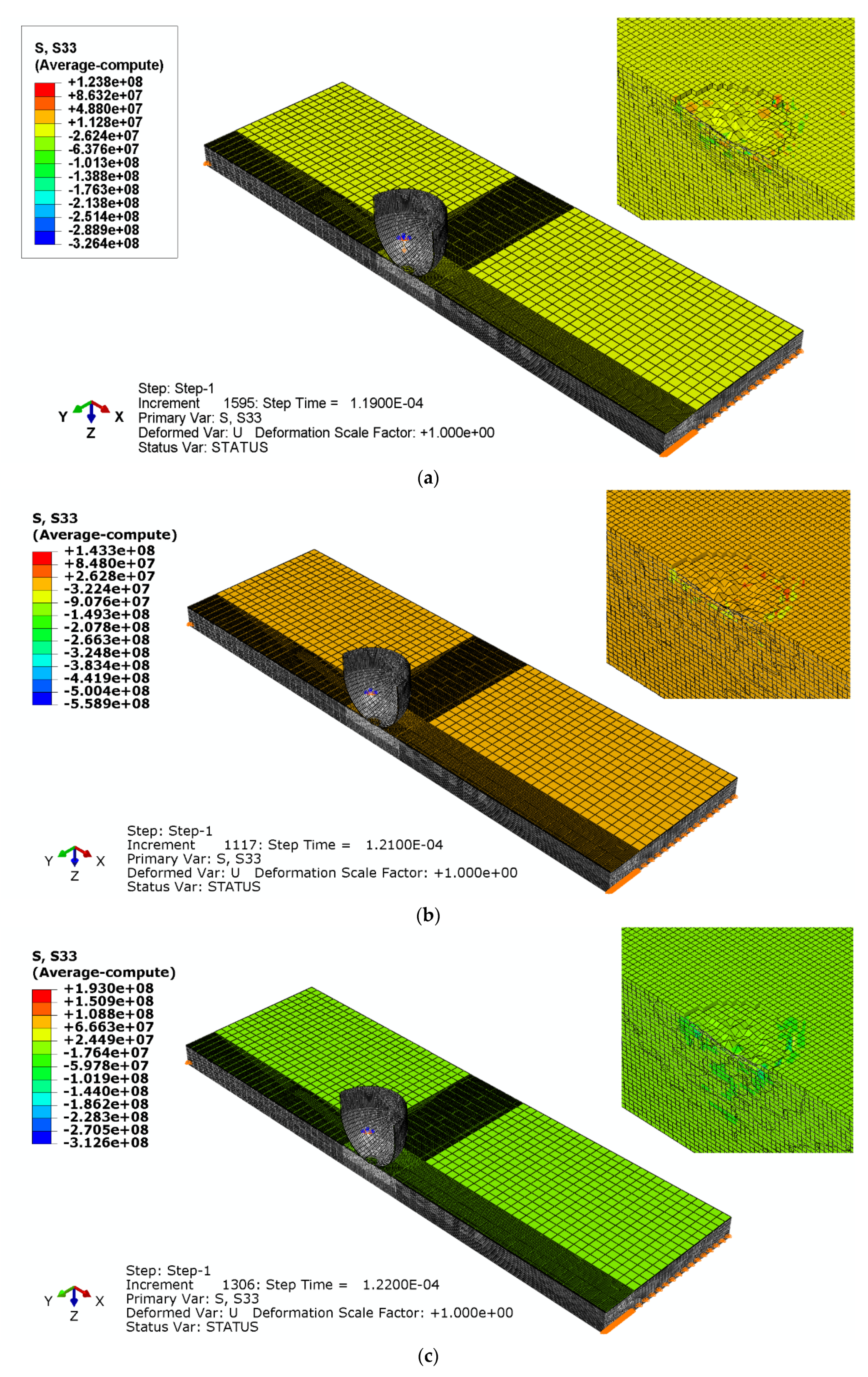
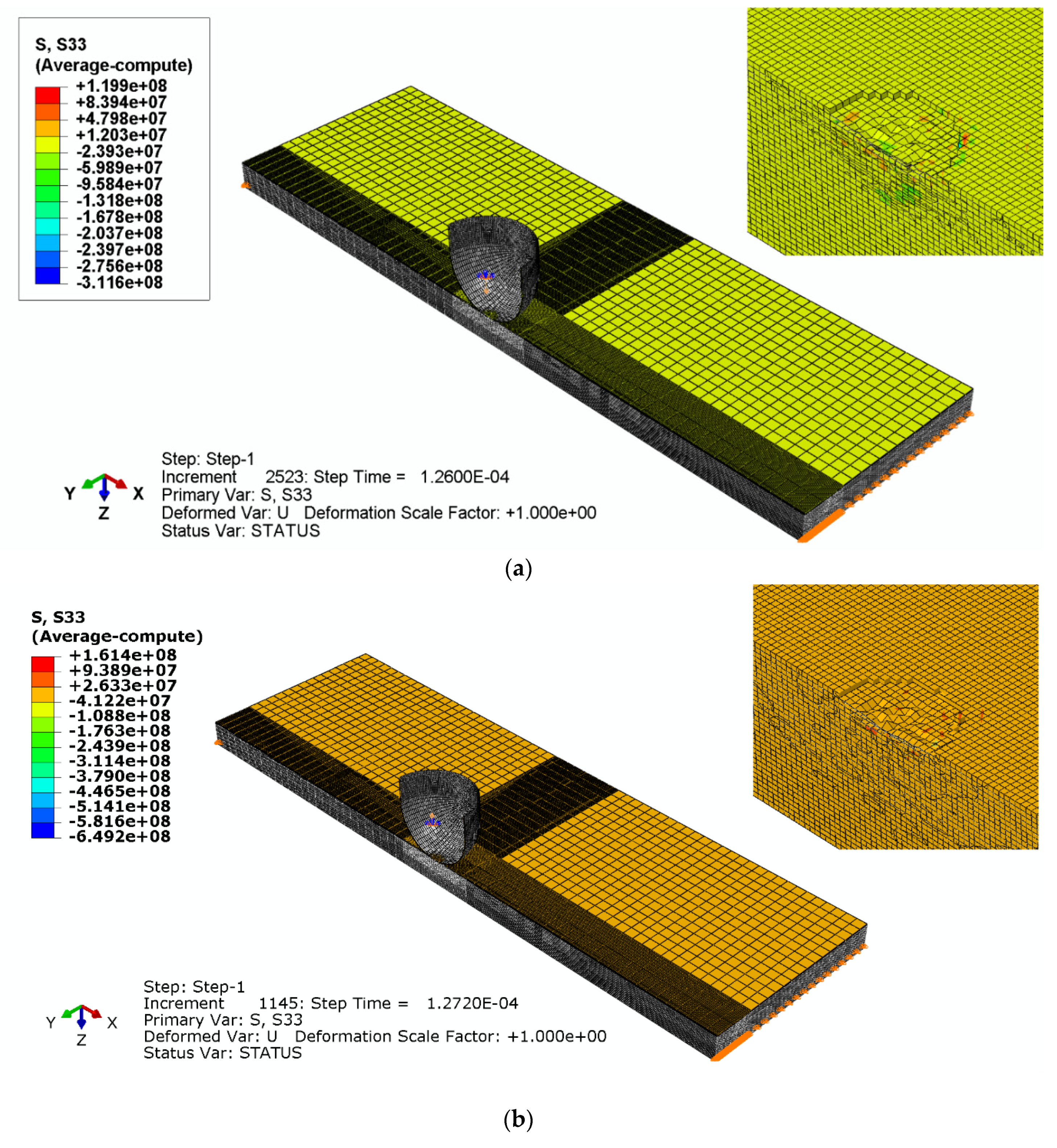
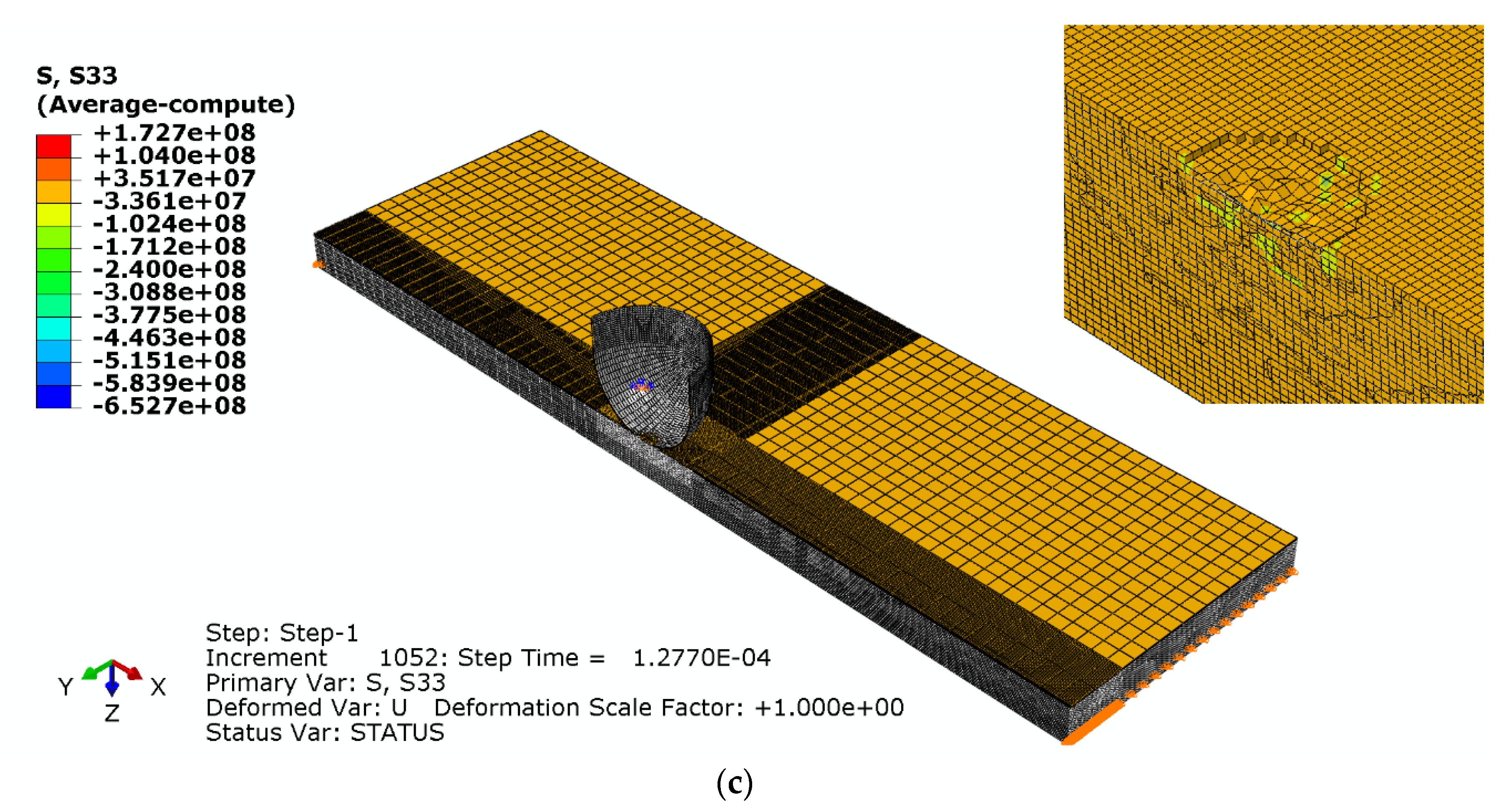
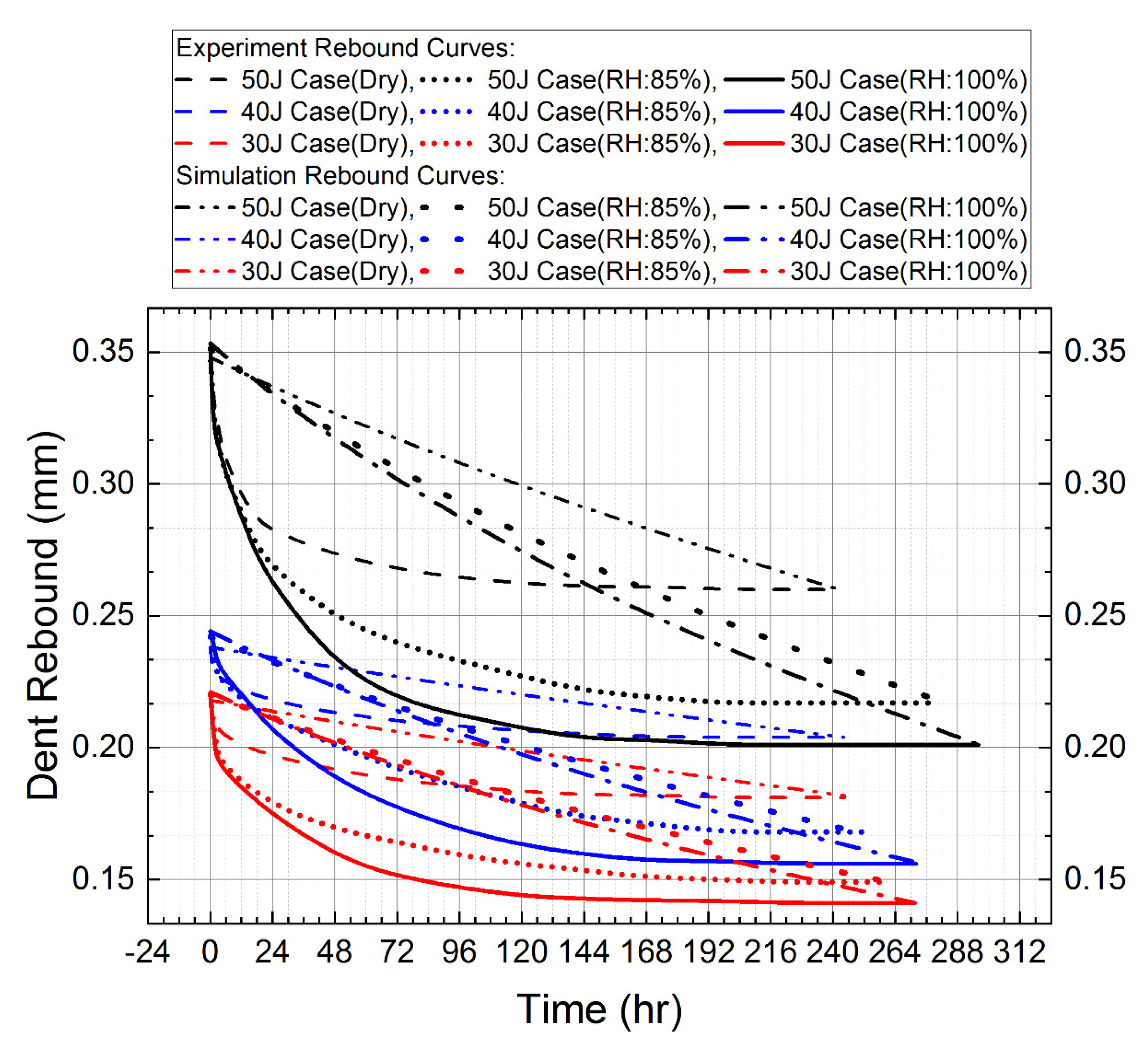
4. Results and Discussion
5. Conclusions
Author Contributions
Funding
Data Availability Statement
Conflicts of Interest
Abbreviations
| LVI | Low Velocity Impact |
| PMC | Polymer Matrix Composite |
| B-K | Benzeggagh–Kenane |
| UMAT | User Material Subroutine for ABAQUS/Standard |
| VUMAT | User Material Subroutine for ABAQUS/Explicit |
| CFRP | Carbon Fiber Reinforced Polymer |
| CZM | Cohesive Zone Modeling |
| VCCT | Virtual Crack Closure Technique |
| CDM | Continuum Damage Mechanics |
| UD | Unidirectional |
| GRP | Glass Reinforced Plastic |
| FRC | Fiber Reinforced Concrete |
| TS | Thermoset |
| TP | Thermoplastic |
| AE | Acoustic Emission |
| NDT | Non-Destructive Testing |
| LCA | Life Cycle Analysis |
References
- Choi, H.Y.; Chang, F.K. A model for predicting damage in graphite/epoxy laminated composites resulting from low-velocity point impact. J. Compos. Mater. 1992, 26, 2134–2169. [Google Scholar] [CrossRef]
- Brewer, J.C.; Lagace, P.A. Quadratic stress criterion for initiation of delamination. J. Compos. Mater. 1988, 22, 1141–1155. [Google Scholar] [CrossRef]
- Tita, V.; Carvalho, J.; Vandepitte, D. Failure analysis of low velocity impact on thin composite laminates: Experimental and numerical approaches. Compos. Struct. 2008, 83, 413–428. [Google Scholar] [CrossRef]
- Farooq, U.; Myler, P. Efficient computational modelling of carbon fibre reinforced laminated composite panels subjected to low velocity drop-weight impact. Mater. Des. 2014, 54, 43–56. [Google Scholar] [CrossRef]
- Fleming, D.C. Delamination Modeling of Composites for Improved Crash Analysis; NASA/CR-1999-209725; National Aeronautics and Space Administration, Langley Research Center: Hampton, VA, USA, 1999. [Google Scholar]
- Ronald, K. Virtual crack closure technique: History, approach, and applications. Appl. Mech. Rev. 2004, 57, 109–143. [Google Scholar]
- Aymerich, F.; Dore, F.; Priolo, P. Prediction of impact-induced delamination in cross-ply composite laminates using cohesive interface elements. Compos. Sci. Technol. 2008, 68, 2383–2390. [Google Scholar] [CrossRef] [Green Version]
- Shi, Y.; Soutis, C. A finite element analysis of impact damage in composite laminates. Aeronaut. J. 2012, 116, 1131–1147. [Google Scholar] [CrossRef]
- Caputo, F.; De Luca, A.; Lamanna, G.; Borrelli, R.; Mercurio, U. Numerical study for the structural analysis of composite laminates subjected to low velocity impact. Compos. Part B 2014, 67, 296–302. [Google Scholar] [CrossRef]
- Bouvet, C.; Castanié, B.; Bizeul, M.; Barrau, J.J. Low velocity impact modelling in laminate composite panels with discrete interface elements. Int. J. Solids Struct. 2009, 46, 2809–2821. [Google Scholar] [CrossRef] [Green Version]
- Donadon, M.V.; Iannucci, L.; Falzon, B.G.; Hodgkinson, J.M.; de Almeida, S.F. A progressive failure model for composite laminates subjected to low velocity impact damage. Comput. Struct. 2008, 86, 1232–1252. [Google Scholar] [CrossRef]
- Kim, E.H.; Rim, M.S.; Lee, I.; Hwang, T.K. Composite damage model based on continuum damage mechanics and low velocity impact analysis of composite plates. Compos. Struct. 2013, 95, 123–134. [Google Scholar] [CrossRef]
- Riccio, A.; De Luca, A.; Di Felice, G.; Caputo, F. Modelling the simulation of impact induced damage onset and evolution in composites. Compos. Part B 2014, 66, 340–347. [Google Scholar] [CrossRef]
- Batra, R.C.; Gopinath, G.; Zheng, J.Q. Damage and failure in low energy impact of fiber-reinforced polymeric composite laminates. Compos. Struct. 2012, 94, 540–547. [Google Scholar] [CrossRef]
- Zubillaga, L.; Turon, A.; Maimi, P.; Costa, J.; Mahdi, S.; Linde, P. An energy based failure criterion for matrix crack induced delamination in laminated composite structures. J. Compos. Struct. 2014, 112, 339–344. [Google Scholar] [CrossRef]
- Bouvet, C.; Rivallant, S. Damage tolerance of composite structures under low-velocity impact. In Dynamic Deformation, Damage and Fracture in Composite Materials and Structures; Woodhead Publishing: Cambridge, UK, 2016. [Google Scholar] [CrossRef]
- Luo, G.M.; Lee, Y.J. Quasi-static simulation of constrained layered damped laminated curvature shells subjected to low-velocity impact. Compos. Part B 2011, 42, 1233–1243. [Google Scholar] [CrossRef]
- Sutherland, L.S.; Guedes Soares, C. The use of quasi-static testing to obtain the low-velocity impact damage resistance of marine GRP laminates. Compos. Part B 2012, 43, 1459–1467. [Google Scholar] [CrossRef]
- Yokozeki, T.; Kuroda, A.; Yoshimura, A.; Ogasawara, T.; Aoki, T. Damage characterization in thin-ply composite laminates under out-of-plane transverse loadings. Compos. Struct. 2010, 93, 49–57. [Google Scholar] [CrossRef]
- Brindle, A.R.; Zhang, X. Predicting the compression-after-impact performance of carbon fibre composites based on impact response. In Proceedings of the 17th International Conference on Composite Materials (ICCM17), Edinburgh, UK, 27–31 July 2009. [Google Scholar]
- Yigit, A.S.; Christoforou, A.P. Limits of asymptotic solutions in low-velocity impact of composite plates. Compos. Struct. 2007, 81, 568–574. [Google Scholar] [CrossRef]
- Wagih, A.; Maimí, P.; Blanco, N.; González, E.V. Scaling effects of composite laminates under out-of-plane loading. Compos. Part A Appl. Sci. Manuf. 2019, 16, 1–12. [Google Scholar] [CrossRef]
- Karakuzu, R.; Erbil, E.; Aktas, M. Impact characterization of glass/epoxy composite plates: An experimental and numerical study. Compos. Part B 2010, 41, 388–395. [Google Scholar] [CrossRef]
- Caprino, G.; Langella, A.; Lopresto, A. Indentation and penetration of carbon fibre reinforced plastic laminates. Compos. Part B 2003, 34, 319–325. [Google Scholar] [CrossRef]
- He, W.; Guan, Z.; Li, X.; Liu, D. Prediction of permanent indentation due to impact on laminated composites based on an elasto-plastic model incorporating fiber failure. Compos. Struct. 2013, 96, 232–242. [Google Scholar] [CrossRef]
- Xiao, L.; Wang, G.; Qiu, S.; Han, Z.; Lia, X.; Zhang, D. Exploration of energy absorption and viscoelastic behavior of CFRPs subjected to low velocity impact. Compos. Part B Eng. 2019, 165, 247–254. [Google Scholar] [CrossRef]
- Zobeiry, N.; Malek, S.; Vaziri, R.; Poursartip, A. A differential approach to finite element modelling of isotropic and transversely isotropic viscoelastic materials. Mech. Mater. 2016, 97, 76–91. [Google Scholar] [CrossRef]
- Wagih, A.; Maimí, P.; Blanco, N.; Costa, J. A quasi-static indentation test to elucidate the sequence of damage events in low velocity impacts on composite laminates. Compos. Part A Appl. Sci. Manuf. 2016, 82, 180–189. [Google Scholar] [CrossRef]
- Thomas, M. Study of the evolution of the dent depth due to impact on carbon/epoxy laminates, consequences on impact damage visibility and on in service inspection requirements for civil aircraft composite structures. In Proceedings of the MIL-HDBK 17 Meeting, Monterey, CA, USA, 29–31 March 1994. [Google Scholar]
- Wolff, E.G. Moisture effects on polymer matrix composites. SAMPE J. 1993, 29, 11–19. [Google Scholar]
- Sutherland, L.S. A review of impact testing on marine composite materials: Part III–Damage tolerance and durability. Compos. Struct. 2018, 188, 512–518. [Google Scholar] [CrossRef]
- Berketis, K.; Tzetzis, D.; Hogg, P.J. The influence of long term water immersion ageing on impact damage behaviour and residual compression strength of glass fibre reinforced polymer (GFRP). Mater. Des. 2008, 29, 1300–1310. [Google Scholar] [CrossRef]
- Kimpara, I.; Saito, H. Post-impact fatigue behavior of woven and knitted fabric CFRP laminates for marine use. In Major Accomplishments in Composite Materials and Sandwich Structures; Springer: Dordrecht, The Netherlands, 2009; pp. 113–132. [Google Scholar]
- Strait, L.H.; Karasek, M.L.; Amateau, M.F. Effects of seawater immersion on the impact resistance of glass fiber reinforced epoxy composites. J. Compos. Mater. 1992, 26, 2118–2133. [Google Scholar] [CrossRef]
- Parvatareddy, H.; Tsang, P.W.; Dillard, D. Impact damage resistance and tolerance of high-performance polymeric composites subjected to environmental aging. Compos. Sci. Technol. 1996, 56, 1129–1140. [Google Scholar] [CrossRef]
- Li, G.; Pang, S.S.; Helms, J.E.; Ibekwe, S.I. Low velocity impact response of GFRP laminates subjected to cycling moistures. Polym. Compos. 2000, 21, 686–695. [Google Scholar] [CrossRef]
- Mortas, N.; Er, O.; Reis, P.; Ferreira, J. Effect of corrosive solutions on composites laminates subjected to low velocity impact loading. Compos. Struct. 2014, 108, 205–211. [Google Scholar] [CrossRef]
- Vieille, B.; Aucher, J.; Taleb, L. Comparative study on the behavior of woven-ply reinforced thermoplastic or thermosetting laminates under severe environmental conditions. Mater. Des. 2012, 35, 707–719. [Google Scholar] [CrossRef]
- Castaing, P.; Mallard, H. Effect of plasticization with water on the behaviour of longterm exposed filament wounded composites. In Progress in Durability Analysis of Composite Systems; Cardon, A.H., Fukuda, H., Reifsnider, K., Eds.; Taylor and Francis: Abingdon, UK, 1996; pp. 233–239. [Google Scholar]
- Browning, C.E.; Husman, G.; Whitney, J.M. Moisture Effects in Epoxy Matrix Composites; ASTM special technical publications: West Conshohocken, PA, USA, 1977; pp. 481–496. [Google Scholar]
- Chateauminois, A.; Chabert, B.; Soulier, J.P.; Vincent, L. Hygrothermal ageing effects on viscoelastic and fatigue behaviour of glass/epoxy composites. In Proceedings of the Eighth International Conference on Composite Materials (ICCM8), Honolulu, HI, USA, 15–19 July 1991. [Google Scholar]
- Godin, N.; Reynaud, P.; Fantozzi, G. Acoustic Emission and Durability of Composites Materials; ISTE-Wiley: London, UK, 2018; ISBN 9781786300195. [Google Scholar]
- Barre, S.; Benzeggagh, M. On the use of acoustic emission to investigate damage mechanisms in glass-fiber reinforced polypropylene. Compos. Sci. Technol. 1994, 52, 369–376. [Google Scholar] [CrossRef]
- Chen, O.; Karandikar, P.; Takeda, N.; Kishi, T. Acoustic emission characterization of a glass-matrix composite. Nondestruct. Test. Eval. 1992, 8–9, 869–878. [Google Scholar] [CrossRef]
- Kim, S.-T.; Lee, Y.-T. Characteristics of damage and fracture process of carbon fiber reinforced plastic under loading-unloading test by using AE method. Mater. Sci. Eng. 1997, A234–A236, 322–326. [Google Scholar] [CrossRef]
- Kotsikos, G.; Evans, J.T.; Gibson, A.G.; Hale, J. Use of acoustic emission to characterize corrosion fatigue damage accumulation in glass fiber reinforced polyester laminates. Polym. Compos. 1999, 20, 689–696. [Google Scholar] [CrossRef]
- Kaliske, M.; Rothert, H. Formulation and implementation of three-dimensional viscoelasticity at small and finite strains. Comput. Mech. 1997, 19, 228–239. [Google Scholar] [CrossRef]
- Yousaf, M.; Zhou, C. Numerical Study on the Rebound of Low-Velocity Impact-Induced Indentation in Composite Laminate. Aerospace 2022, 9, 651. [Google Scholar] [CrossRef]
- Zhang, J.; Zhang, X. An efficient approach for predicting low-velocity impact force and damage in composite laminates. Compos. Struct. 2015, 130, 85–94. [Google Scholar] [CrossRef]
- Benzeggagh, M.L.; Kenane, M. Measurement of mixed-mode delamination fracture toughness of unidirectional glass/epoxy composites with mixed-mode bending apparatus. J. Compos. Sci. Technol. 2003, 56, 439–449. [Google Scholar] [CrossRef]
- Camanho, P.P.; Davila, C.G.; De Moura, M.F. Numerical simulation of mixed-mode progressive delamination in composite materials. J. Compos. Mater. 2003, 37, 1415–1438. [Google Scholar] [CrossRef]
- D 5229/D 5229M-92; Standard Test Method for Moisture Absorption Properties and Equilibrium Conditioning of Polymer Matrix Composite Materials. ASTM International: West Conshohocken, PA, USA, 2004.
- ASTM D7136; Standard Test METHOD for Measuring the Damage Resistance of a Fiber Reinforced Polymer Matrix Composite to a Drop-Weight Impact Event. Annual Book of ASTM Standards. ASTM International: West Conshohocken, PA, USA, 2015; pp. 1–16.


| Damage Type | Failure Mode | Damage Initiation | |
|---|---|---|---|
| Lamina Ply Level | Matrix | Tension Cracking | |
| Compression Cracking | |||
| Fiber | Tension Failure | ||
| Compression Failure | |||
| Damage Type | Damage Initiation | Damage Propagation |
|---|---|---|
| Cohesive Layer Interface | Linear Softening Mixed Mode B-K Law |
| Elastic Constants of a Single UD Ply | Strength of a Single UD Ply |
|---|---|
| E1 = 144.62 GPa | = 2612.24 MPa |
| E2 = 9.76 GPa | = 1583.47 MPa |
| G12 = 5.44 GPa | = 58.25 MPa |
| G23 = 3.92 GPa | = 161.76 MPa |
| v12 = 0.31 | = 126.79 MPa |
| v23 = 0.46 | = 91.84 MPa |
(GPa/mm) | (GPa/mm) | (MPa) | (MPa) | (mm) | (mm) | (GPa/mm) | (mm) |
|---|---|---|---|---|---|---|---|
| 1390.0 | 510.0 | 65.5 | 95.5 | 0.014 | 0.025 | 26.5 | 0.043 |
| Dry Specimen at 25 °C Temperature | ||||||
|---|---|---|---|---|---|---|
| Case-I: 50J | Case-II: 40J | Case-III: 30J | ||||
| Time (h) | Depth (mm) | Time (h) | Depth (mm) | Time (h) | Depth (mm) | |
| 0 | 0.348 | 0 | 0.238 | 0 | 0.218 | (di)Dry |
| 0.75 | 0.338 | 0.5 | 0.233 | 0.5 | 0.211 | |
| 4 | 0.311 | 1 | 0.229 | 1.5 | 0.209 | |
| 16 | 0.288 | 4 | 0.226 | 6 | 0.204 | |
| 24 | 0.282 | 14 | 0.221 | 18.33 | 0.198 | |
| 48 | 0.273 | 24 | 0.218 | 50.5 | 0.191 | |
| 76 | 0.267 | 42.5 | 0.214 | 77.5 | 0.187 | |
| 100 | 0.264 | 51 | 0.213 | 101.33 | 0.185 | |
| 124 | 0.262 | 72 | 0.210 | 125.5 | 0.183 | |
| 148 | 0.261 | 98 | 0.208 | 150 | 0.182 | |
| 172 | 0.261 | 125 | 0.206 | 174 | 0.182 | |
| 196 | 0.260 | 150 | 0.205 | 198.33 | 0.181 | |
| 174 | 0.204 | |||||
| 220 | 0.260 | 198 | 0.204 | 222.33 | 0.181 | |
| 222 | 0.204 | |||||
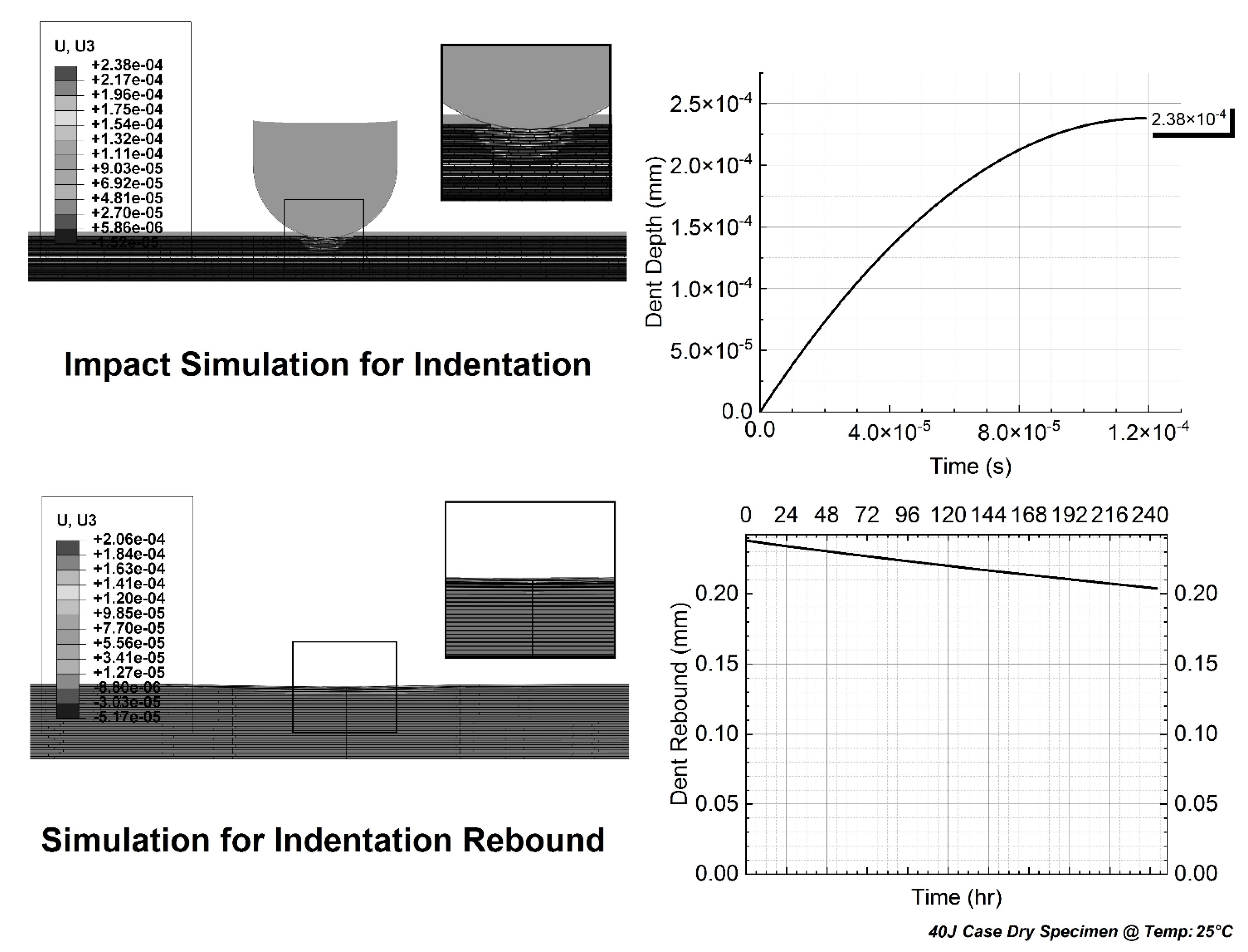
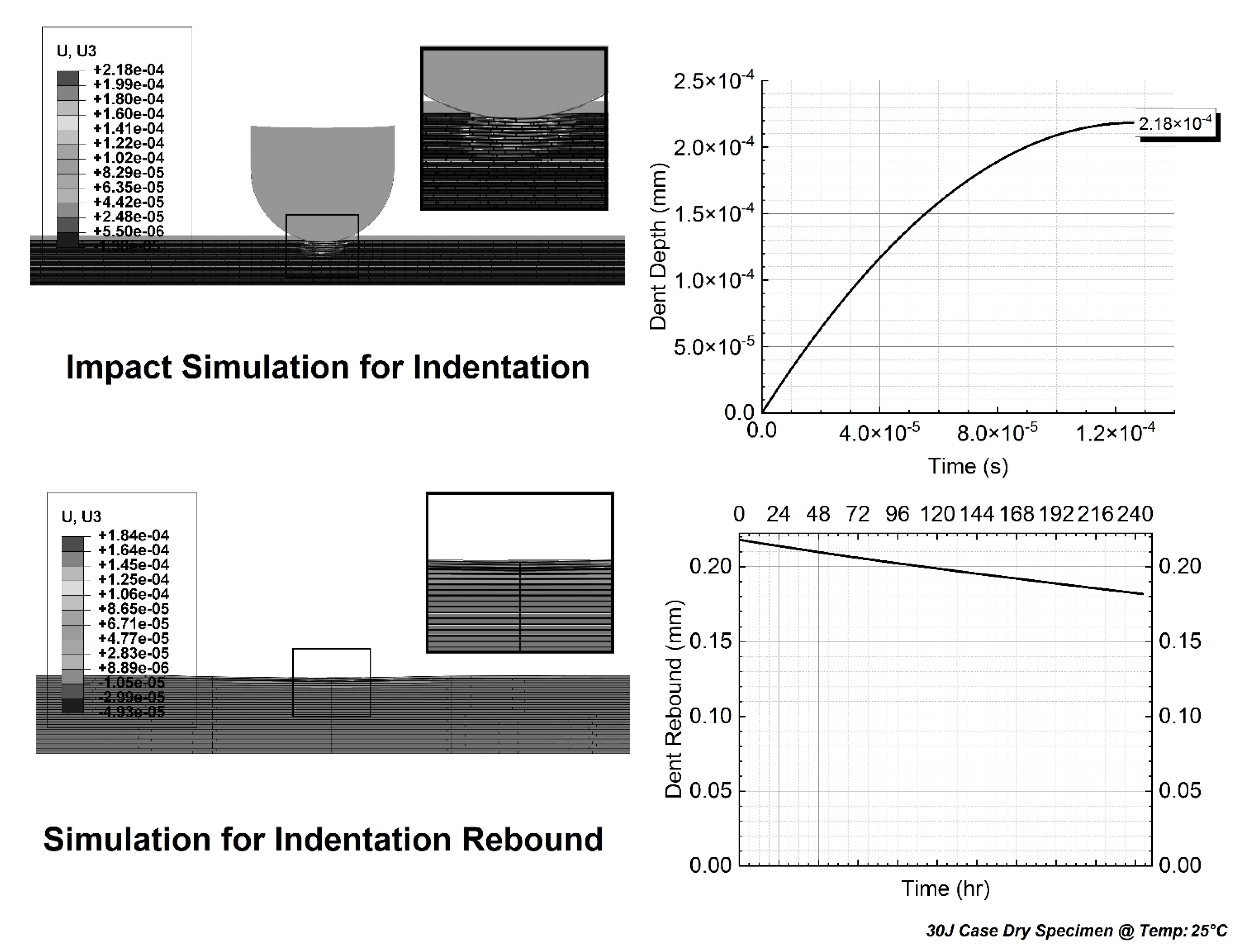
| 242 | 0.260 | 244 | 0.204 | 244.33 | 0.181 | (df)Dry |
| At 25 °C Temperature and RH: 85% | ||||||
|---|---|---|---|---|---|---|
| Case-I: 50J | Case-II: 40J | Case-III: 30J | ||||
| Time (h) | Depth (mm) | Time (h) | Depth (mm) | Time (h) | Depth (mm) | |
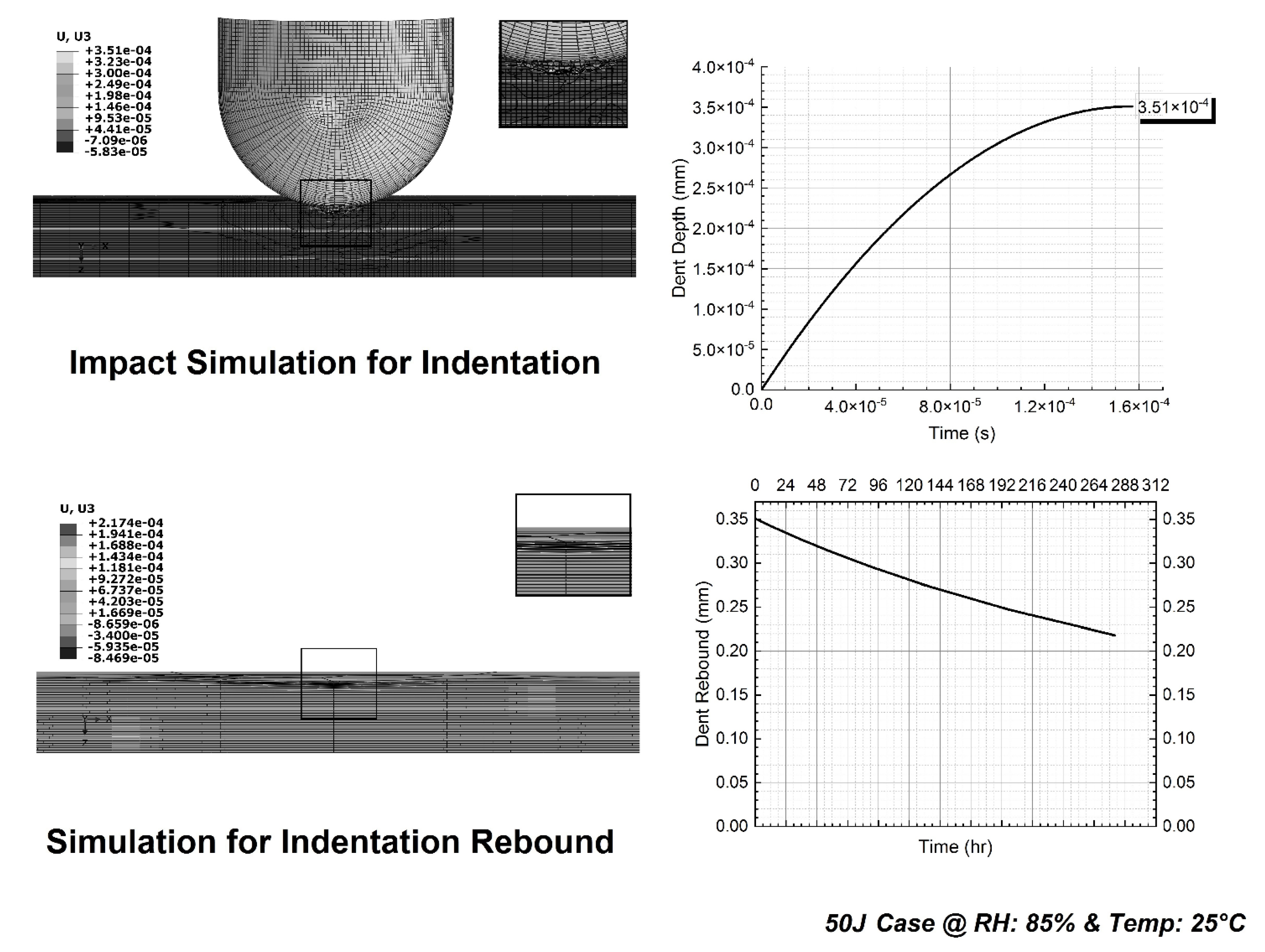
| 0 | 0.351 | 0 | 0.242 | 0 | 0.220 | |
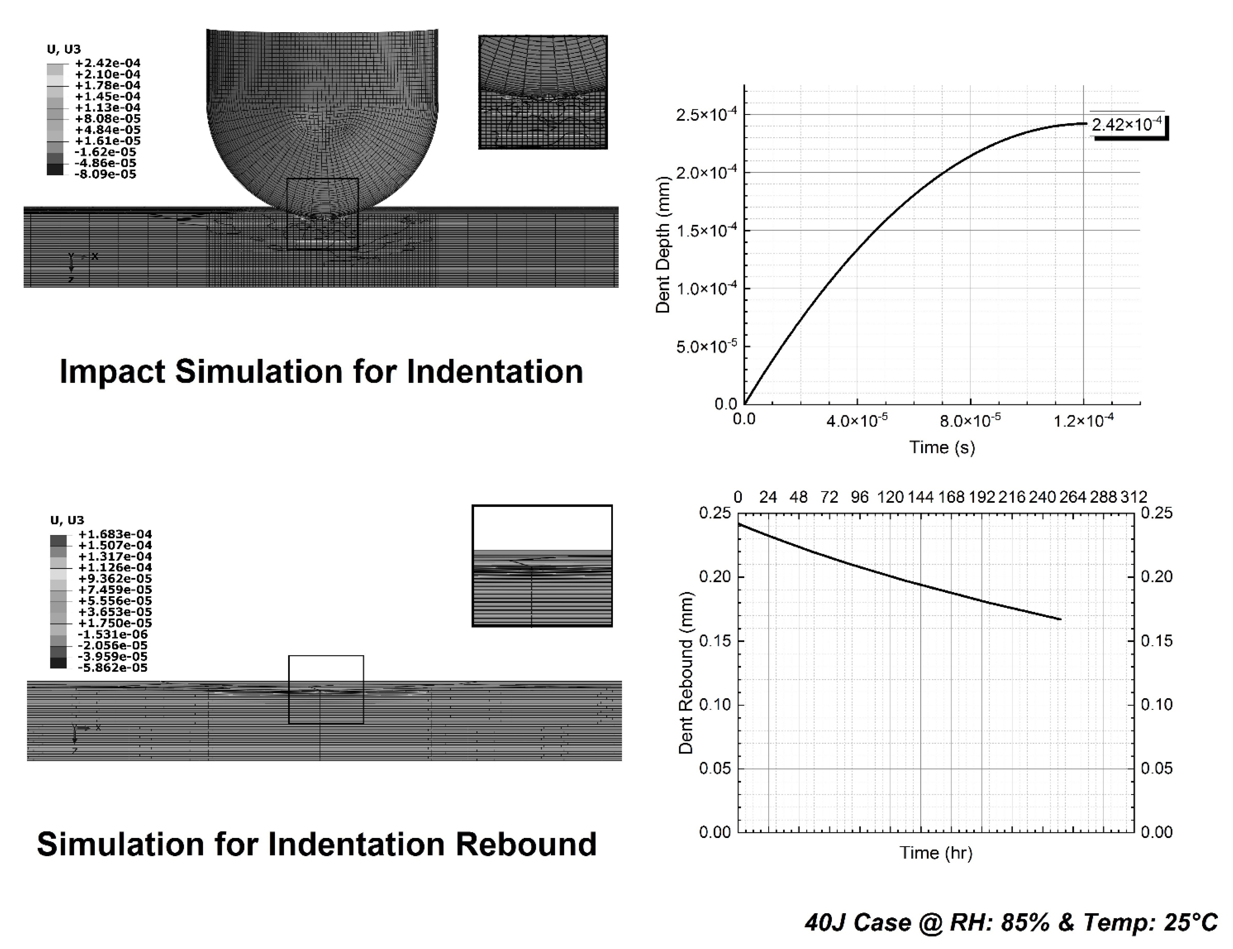
| 1 | 0.329 | 1 | 0.238 | 1 | 0.212 | |
| 3 | 0.310 | 2 | 0.230 | 2 | 0.201 | |
| 16 | 0.279 | 4 | 0.225 | 4 | 0.194 | |
| 24 | 0.268 | 18 | 0.214 | 18 | 0.182 | |
| 48 | 0.249 | 24 | 0.211 | 40 | 0.171 | |
| 76 | 0.238 | 48 | 0.201 | 72 | 0.164 | |
| 100 | 0.232 | 72 | 0.192 | 108 | 0.157 | |
| 124 | 0.226 | 96 | 0.185 | 140 | 0.154 | |
| 148 | 0.221 | 120 | 0.179 | 166 | 0.151 | |
| 172 | 0.219 | 140 | 0.174 | 196 | 0.15 | |
| 196 | 0.217 | 172 | 0.171 | 220 | 0.149 | |
| 220 | 0.217 | 198 | 0.168 | 248 | 0.149 | |
| 244 | 0.217 | 220 | 0.168 | |||
| 268 | 0.217 | |||||
| 280 | 0.217 | 254 | 0.168 | 260 | 0.149 | |
| At 25 °C Temperature and RH: 100% | ||||||
|---|---|---|---|---|---|---|
| Case-I: 50J | Case-II: 40J | Case-III: 30J | ||||
| Time (h) | Depth (mm) | Time (h) | Depth (mm) | Time (h) | Depth (mm) | |
| 0 | 0.353 | 0 | 0.244 | 0 | 0.221 | |
| 1 | 0.325 | 1 | 0.241 | 1 | 0.209 | |
| 3 | 0.312 | 2 | 0.235 | 2 | 0.198 | |
| 16 | 0.276 | 4 | 0.229 | 4 | 0.192 | |
| 24 | 0.262 | 16 | 0.216 | 24 | 0.174 | |
| 48 | 0.231 | 24 | 0.206 | 50.5 | 0.158 | |
| 76 | 0.217 | 48 | 0.188 | 72 | 0.151 | |
| 98 | 0.212 | 72 | 0.177 | 108 | 0.145 | |
| 122 | 0.207 | 96 | 0.169 | 132 | 0.143 | |
| 148.5 | 0.203 | 120 | 0.163 | 166 | 0.142 | |
| 170.5 | 0.203 | 148 | 0.159 | 190.5 | 0.142 | |
| 198 | 0.201 | 172 | 0.157 | 224 | 0.141 | |
| 222 | 0.201 | 196 | 0.157 | |||
| 248 | 0.201 | 220 | 0.156 | 248 | 0.141 | |
| 272 | 0.201 | 248 | 0.156 | |||
| 296 | 0.201 | 272 | 0.156 | 271.5 | 0.141 | |
| Hygrothermal Condition | Impact Energy | A1 | t1 | A2 | t2 | y0 | Adj. R-Square |
|---|---|---|---|---|---|---|---|
| 25 °C, Dry Specimen [47] | 50J Case | 0.04918 | 3.48385 | 0.03910 | 44.22815 | 0.25979 | 0.99989 |
| 40J Case | 0.01135 | 0.78406 | 0.02320 | 54.84134 | 0.20355 | 0.99823 | |
| 30J Case | 0.01074 | 0.74417 | 0.02614 | 52.47742 | 0.18074 | 0.99644 | |
| 25 °C, RH: 85% | 50J Case | 0.05212 | 2.38215 | 0.08222 | 56.32780 | 0.21584 | 0.99888 |
| 40J Case | 0.01713 | 2.18399 | 0.06377 | 92.10215 | 0.16190 | 0.99726 | |
| 30J Case | 0.02978 | 2.37639 | 0.04347 | 70.98319 | 0.14747 | 0.99808 | |
| 25 °C, RH: 100% | 50J Case | 0.03347 | 0.76271 | 0.11800 | 36.08439 | 0.20149 | 0.99932 |
| 40J Case | 0.00987 | 1.92337 | 0.08031 | 55.13927 | 0.15452 | 0.99905 | |
| 30J Case | 0.02600 | 1.44405 | 0.05480 | 44.42592 | 0.14066 | 0.99880 |
| Relative Humidity (% RH) | Temperature (°C) | Pressure (atm, mm of Hg) | Moisture Content (g/m3) | Mass Concentration (ppmv) | Volume (% v) |
|---|---|---|---|---|---|
| 85 | 25 | 1, 760 | 20 | 27430 | 2.74 |
| 100 | 25 | 1, 760 | 23 | 32427 | 3.24 |
| Impact Energy (J) | |||
|---|---|---|---|
| 50 | 40 | 30 | |
| Velocity (m/s) | 4.47 | 4.00 | 3.46 |
| Hygrothermal Condition | Material Type | α |
|---|---|---|
| 25 °C/RH: 85% | UD Laminae Ply | 0.1420 GPa |
| Cohesive Interface | 1.3622 GPa/mm | |
| 25 °C/RH: 100% | UD Laminae Ply | 0.1880 GPa |
| Cohesive Interface | 1.8070 GPa/mm |
| Impact Case | ABAQUS Explicit Analysis | ABAQUS Standard Analysis | |||
|---|---|---|---|---|---|
| Loading Step Time (ms) | Max Pressure (Pa) | Initial Indentation Depth (mm) | Rebound Step Time (h) | Final Indentation Depth (mm) | |
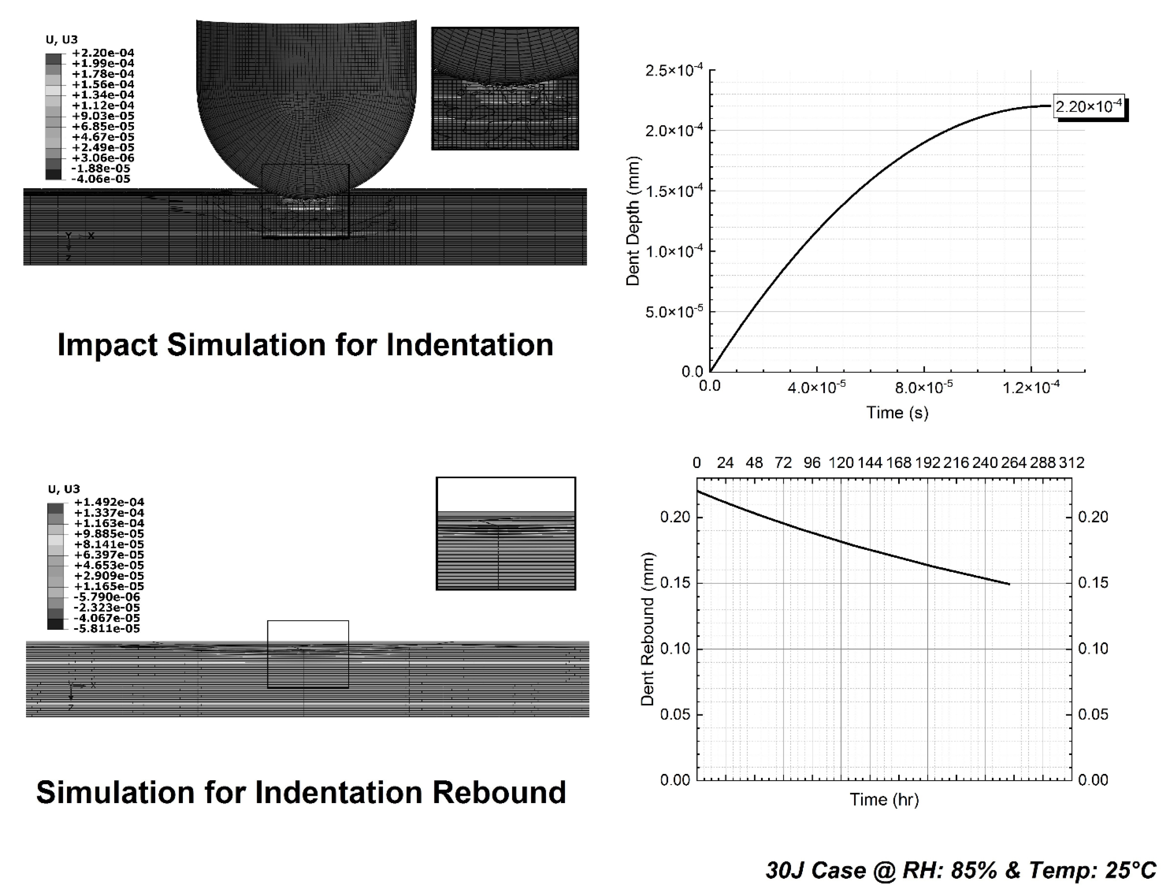
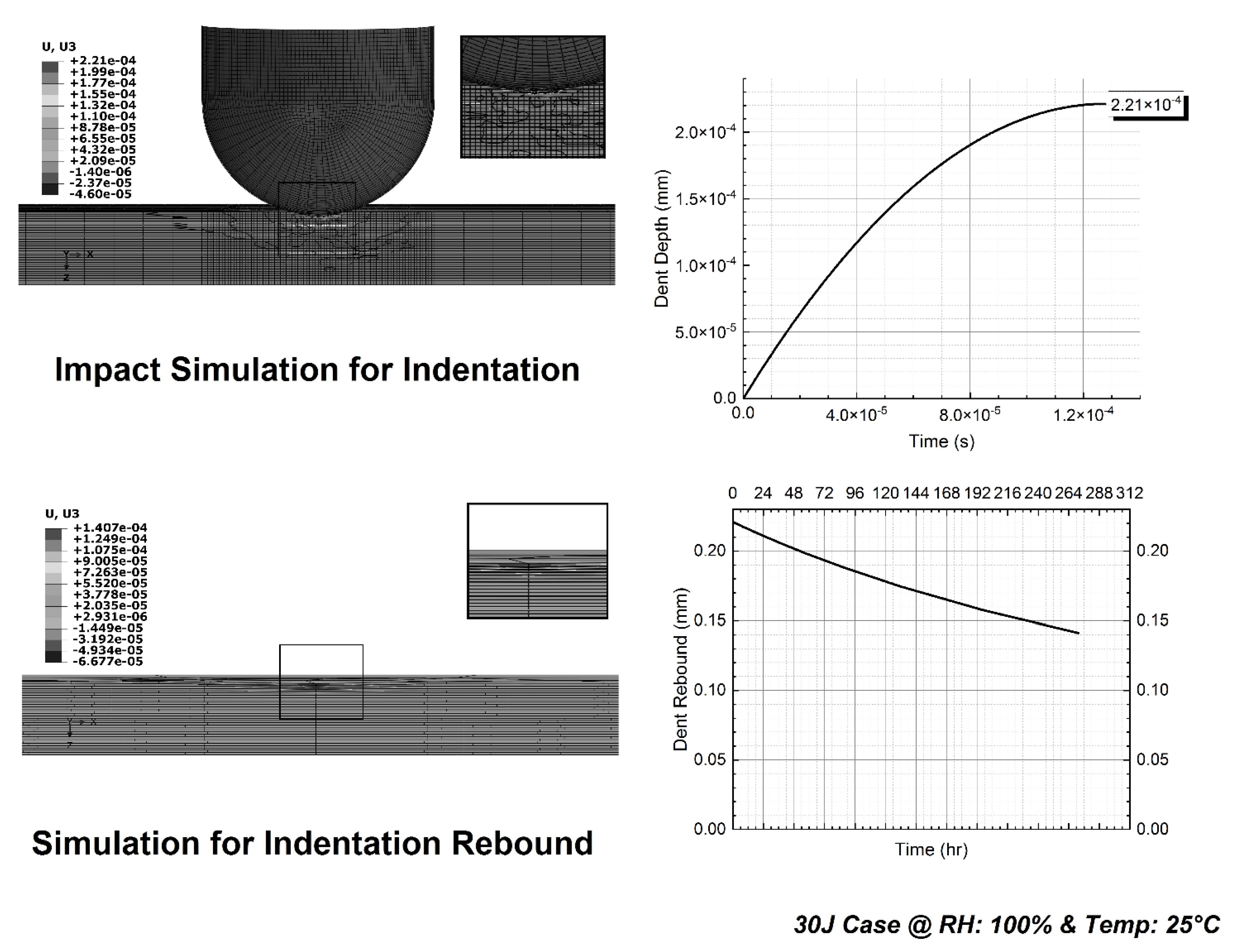
| Case-I: 50J | 0.155 | 4.8 × 10⁸ | 0.348 | 242 | 0.260 |
| Case-II: 40J | 0.119 | 4.4 × 10⁸ | 0.238 | 244 | 0.204 |
| Case-III: 30J | 0.126 | 4.1 × 10⁸ | 0.218 | 244.33 | 0.181 |
| Impact Case | ABAQUS Explicit Analysis | ABAQUS Standard Analysis | |||
|---|---|---|---|---|---|
| Loading Step Time (ms) | Max Contact Pressure (Pa) | Initial Indentation Depth (mm) | Rebound Step Time (h) | Final Indentation Depth (mm) | |
| Case-I: 50J | 0.157 | 4.5 × 10⁸ | 0.351 | 280 | 0.217 |
| Case-II: 40J | 0.121 | 4.6 × 10⁸ | 0.242 | 254 | 0.168 |
| Case-III: 30J | 0.1272 | 3.4 × 10⁸ | 0.220 | 260 | 0.149 |
| Impact Case | ABAQUS Explicit Analysis | ABAQUS Standard Analysis | |||
|---|---|---|---|---|---|
| Loading Step Time (ms) | Max Contact Pressure (Pa) | Initial Indentation Depth (mm) | Rebound Step Time (h) | Final Indentation Depth (mm) | |
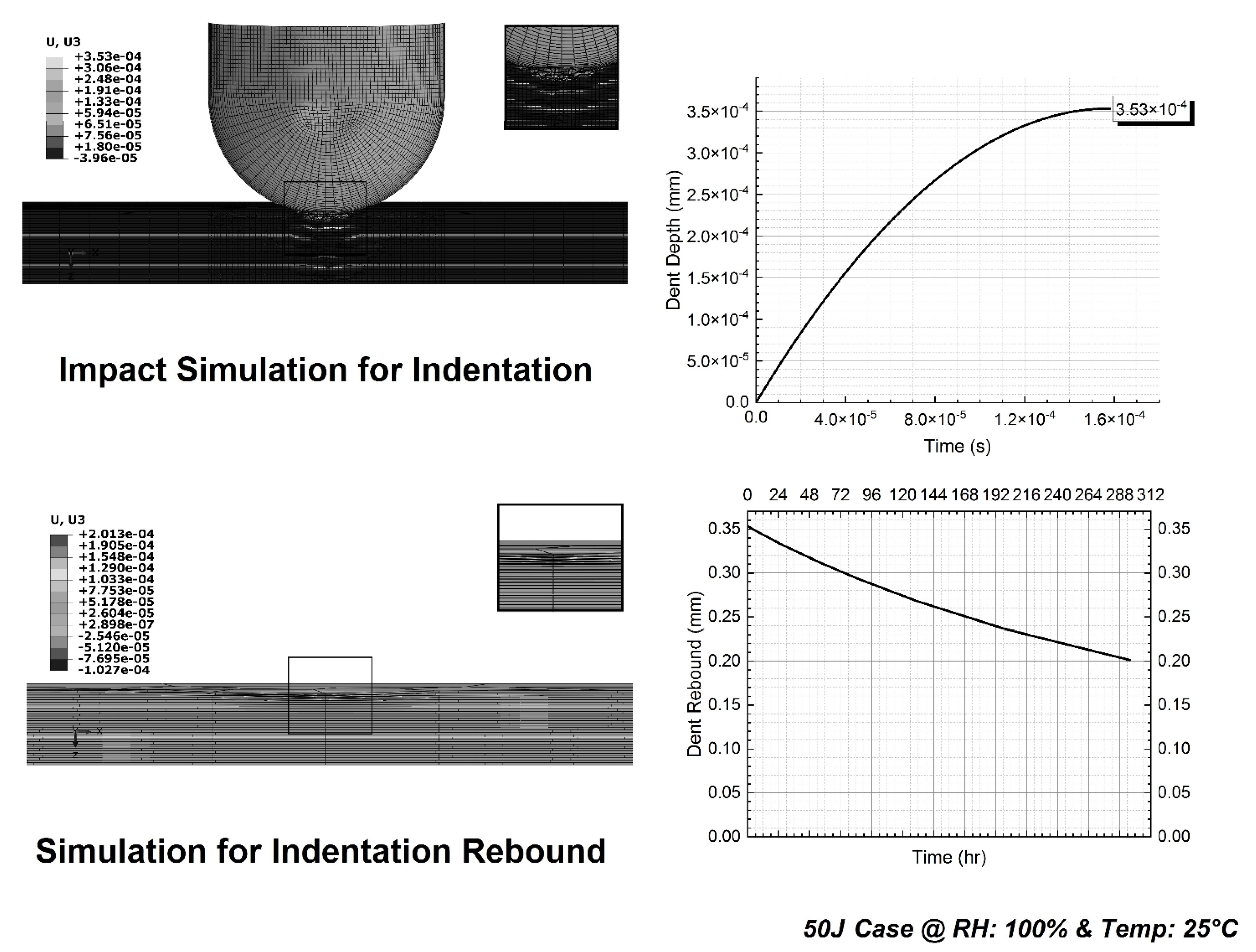
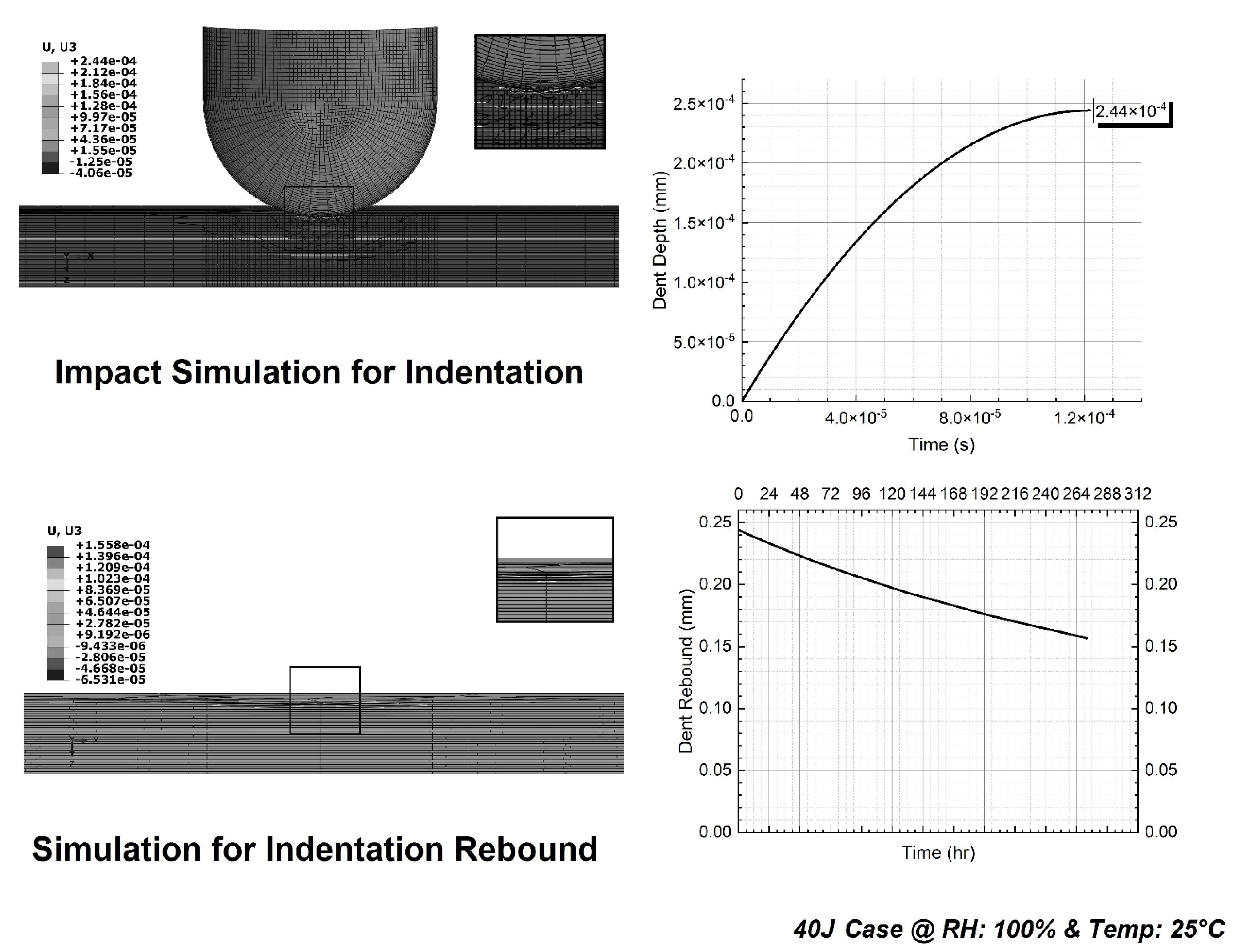
| Case-I: 50J | 0.158 | 6.0 × 10⁸ | 0.353 | 296 | 0.201 |
| Case-II: 40J | 0.122 | 4.9 × 10⁸ | 0.244 | 272 | 0.156 |
| Case-III: 30J | 0.1277 | 3.7 × 10⁸ | 0.221 | 271.5 | 0.141 |
| Impact Case | Material Type | 1st Maxwell Chain | 2nd Maxwell Chain | ||||
|---|---|---|---|---|---|---|---|
| Time 1 (h) | Value 1 (GPa) | Time 2 (h) | Value 2 (GPa) | ||||
| Case-I: 50J | UD Laminae Ply | 240 | 100 | 14 | 2 × 10⁷ | ||
| Cohesive Interface | 240 | Value 1 | Value 1 | 14 | Value 2 | Value 2 | |
| 55.208 | 9.331 | 1.68 × 10⁸ | 2.85 × 10⁷ | ||||
| Case-II: 40J | UD Laminae Ply | 240 | 100 | 21 | 2 × 10⁷ | ||
| Cohesive Interface | 240 | 55.208 | 9.331 | 21 | 1.93 × 10⁸ | 3.27 × 10⁷ | |
| Case-III: 30J | UD Laminae Ply | 240 | 100 | 16 | 2 × 10⁷ | ||
| Cohesive Interface | 240 | 55.208 | 9.331 | 16 | 2.15 × 10⁸ | 3.64 × 10⁷ | |
| Hygrothermal Condition | Rebound Case | Material Type | α | β |
|---|---|---|---|---|
| 25 °C/RH:85% | Case-I: 50J | UD Laminae Ply | The same as in Table 11 | 0.335 |
| Cohesive Interface | ||||
| Case-II: 40J | UD Laminae Ply | 0.580 | ||
| Cohesive Interface | ||||
| Case-III: 30J | UD Laminae Ply | 0.535 | ||
| Cohesive Interface | ||||
| 25 °C/RH:100% | Case-I: 50J | UD Laminae Ply | The same as in Table 11 | 0.400 |
| Cohesive Interface | ||||
| Case-II: 40J | UD Laminae Ply | 0.630 | ||
| Cohesive Interface | ||||
| Case-III: 30J | UD Laminae Ply | 0.580 | ||
| Cohesive Interface |
| Dry Specimen at 25 °C Temperature | |||||
|---|---|---|---|---|---|
| Impact Energy Case | Total Dent Rebound (mm) | Way Out | Experimental Result | Simulation Result | Prediction Accuracy |
| Case-I: 50J | 0.088 | Initial and final dent depths | Matched | Matched | Accurately predicted |
| Dent rebound path | The curve is decaying at a faster rate and soon stops decaying before the final point | The curve is decaying at a slower rate and never stops decaying until the final point | Poor prediction Max error: 19.35% | ||
| Case-II: 40J | 0.034 | Initial and final dent depths | Matched | Matched | Accurately predicted |
| Dent rebound path | The curve is decaying at a faster rate and soon stops decaying before the final point | The curve is decaying at a slower rate and never stops decaying until the final point | Fairly inaccurate prediction Max error: 7.97% | ||
| Case-III: 30J | 0.037 | Initial and final dent depths | Matched | Matched | Accurately predicted |
| Dent rebound path | The curve is decaying at a faster rate and soon stops decaying before the final point | The curve is decaying at a slower rate and never stops decaying until the final point | Fairly inaccurate prediction Max error: 9.88% | ||
| Specimen at 25 °C Temperature and RH: 85% | |||||
|---|---|---|---|---|---|
| Impact Case | Total Dent Rebound (mm) | Way Out | Experimental Result | Simulation Result | Prediction Accuracy |
| Case-I: 50J | 0.134 | Initial and final dent depths | Matched | Matched | Accurately predicted |
| Dent rebound path | Curve is decaying at a faster rate and soon stops decaying before the final point | Curve is decaying at a slower rate and never stops decaying until the final point | Poor prediction Max error: 28.36% | ||
| Case-II: 40J | 0.074 | Initial and final dent depths | Matched | Matched | Accurately predicted |
| Dent rebound path | Curve is decaying at a faster rate and soon stops decaying before the final point | Curve is decaying at a slower rate and never stops decaying until the final point | Fairly inaccurate prediction Max error: 12.29% | ||
| Case-III: 30J | 0.071 | Initial and final dent depths | Matched | Matched | Accurately predicted |
| Dent rebound path | Curve is decaying at a faster rate and soon stops decaying before the final point | Curve is decaying at a slower rate and never stops decaying until the final point | Inaccurate prediction Max error: 20.36% | ||
| Specimen at 25 °C Temperature and RH: 100% | |||||
|---|---|---|---|---|---|
| Impact Case | Total Dent Rebound (mm) | Way Out | Experimental Result | Simulation Result | Prediction Accuracy |
| Case-I: 50J | 0.152 | Initial and final dent depths | Matched | Matched | Accurately predicted |
| Dent rebound path | Curve is decaying at a faster rate and soon stops decaying before the final point | Curve is decaying at a slower rate and never stops decaying until the final point | Poor prediction Max error: 37.90% | ||
| Case-II: 40J | 0.088 | Initial and final dent depths | Matched | Matched | Accurately predicted |
| Dent rebound path | Curve is decaying at a faster rate and soon stops decaying before the final point | Curve is decaying at a slower rate and never stops decaying until the final point | Inaccurate prediction Max error: 21.50% | ||
| Case-III: 30J | 0.080 | Initial and final dent depths | Matched | Matched | Accurately predicted |
| Dent rebound path | Curve is decaying at a faster rate and soon stops decaying before the final point | Curve is decaying at a slower rate and never stops decaying until the final point | Poor prediction Max error: 28.04% | ||
Publisher’s Note: MDPI stays neutral with regard to jurisdictional claims in published maps and institutional affiliations. |
© 2022 by the authors. Licensee MDPI, Basel, Switzerland. This article is an open access article distributed under the terms and conditions of the Creative Commons Attribution (CC BY) license (https://creativecommons.org/licenses/by/4.0/).
Share and Cite
Yousaf, M.; Zhou, C.; Yang, Y.; Wang, L. Numerical Study of the Hygrothermal Effects on Low Velocity Impact Induced Indentation and Its Rebound in Composite Laminate. Aerospace 2022, 9, 802. https://doi.org/10.3390/aerospace9120802
Yousaf M, Zhou C, Yang Y, Wang L. Numerical Study of the Hygrothermal Effects on Low Velocity Impact Induced Indentation and Its Rebound in Composite Laminate. Aerospace. 2022; 9(12):802. https://doi.org/10.3390/aerospace9120802
Chicago/Turabian StyleYousaf, Muhammad, Chuwei Zhou, Yu Yang, and Li Wang. 2022. "Numerical Study of the Hygrothermal Effects on Low Velocity Impact Induced Indentation and Its Rebound in Composite Laminate" Aerospace 9, no. 12: 802. https://doi.org/10.3390/aerospace9120802