Article

A Novel Fuzzy-SAE Control Method for an Improved Test Wind Tunnel Simulating Sand/Dust Environment

National Key Laboratory of Human Machine and Environment Engineering, School of Aeronautical Science and Engineering, Beihang University, Beijing 100191, China
*
Author to whom correspondence should be addressed.
Aerospace 2022, 9(12), 784; https://doi.org/10.3390/aerospace9120784
Submission received: 27 August 2022 / Revised: 17 November 2022 / Accepted: 21 November 2022 / Published: 1 December 2022

Abstract

:
The sand/dust environment is an important cause of aircraft failure. A sand/dust environment simulation experiment must be devised to meet the standard technical requirements. Therefore, this article designs the control system for a sand/dust environment test tunnel, including a wind speed control system and a pneumatic conveying and concentration control system. A fuzzy intelligent control method and a deep neural network are used to track and control experimental parameters. Compared to the classic PID algorithm, this method achieves smaller overshoot, faster response speed, no steady error and a better dynamic response curve, as demonstrated by both the test result in the wind tunnel and a simulation result. Both the classic PID control method and the high-precision fuzzy control method are fast, stable, and robust. The fuzzy-SAE intelligent control method not only has the high accuracy of the classic PID control method but also has the high speed, stability, and robustness of fuzzy control, which can meet the intelligent control requirements of the sand/dust environment test equipment.

1. Introduction

The presence of a sand/dust environment is one of the most important environmental factors that cause aircraft failures [1]. Widespread distribution of sand/dust has a serious impact on the components, systems, and airborne equipment of machinery and aircrafts [2]. The primary types of damage are: erosion, wear, corrosion, and penetration [3]. In light of the laws of dilute gas-solid, harnessing two-phase flow can not only improve the quality of equipment development but also can be used to guide the design and implementation of sand/dust tests and render them more scientific and realistic, which in turn informs the design of sand/dust damage prevention equipment [4]. Meanwhile, it improves the development, production, and identification of weapons and equipment, which has great practical value. At present, it is still difficult to use computers to simulate a sand/dust environment [5]. Therefore, it is essential to construct experimental equipment that simulates such an environment instead.
The standardized sand/dust test conditions are a typical gas-solid two-phase flow field. In the experiment, the concentration of the blowing dust is approximately 10.6 ± 7 g/m3, while the concentration of the blowing sand is between 0.18 ± 0.2 g/m3 and 2.2 ± 0.5 g/m3 [6], in the range of dilute phase transport. Under typical working conditions with a wind speed of 30 m/s, the Reynolds number of the test section will reach 4.47 × 10⁶, which is greater than the critical value of both laminar flow and turbulent flow. The gas is in the turbulent state. Therefore, the flow field in the test device can be considered a dilute-phase turbulent flow and gas-solid two-phase flow.
Designing reliable simulation experiments of a sand/dust environment to meet the requirements is a top priority task [7]. In this article, the effective capacity of the wind tunnel test section and the circulating air volume more than meet the requirements [8]. There is no similar equipment in China that has been specially developed to synthesize blowing sand and blowing dust into a whole device.
To successfully develop such large sand/dust test equipment, solutions must be found for the technical difficulties of temperature, wind speed, and sand/dust concentration control [9]. At the same time, the corrosive sample of the sand/dust should be effectively separated and reclaimed. This will ensure the test equipment’s high reliability and long service life [10]. Therefore, temperature control, wind speed control, sand/dust concentration control, particle distribution uniformity control, and sand/dust reclamation efficiency are the key issues that determine the quality of the developed equipment.
To solve the above problems, B. Barlow presented an experimental method for a low speed wind tunnel [11]. J. Yao offered a control method for wind speed and air flow in a low speed wind tunnel [12]. E. Brown and J. Duhon advanced a concept for designing and testing a full-size helicopter’s air duct [13]. Li Yunze and Yuan Lingshuang developed a control strategy using a Proportion Integration Differentiation (PID) controller in the helicopter’s sand/dust environmental test tunnel [14]. Li Yunze and Yuan Lingshuang proposed a lumped parameter model and control strategy based on the pressure in the wind tunnel [15]. Using the wind tunnel of a helicopter sand/dust test, Ma Zhihong and Yuan Lingshuang formulated a temperature control measurement strategy based on an environmental cooling water flow and electric heater power controller [16]. As for humidity control, Zhang Kaiping outlined a method of dehumidification by controlling the dry compressed air flow [17].
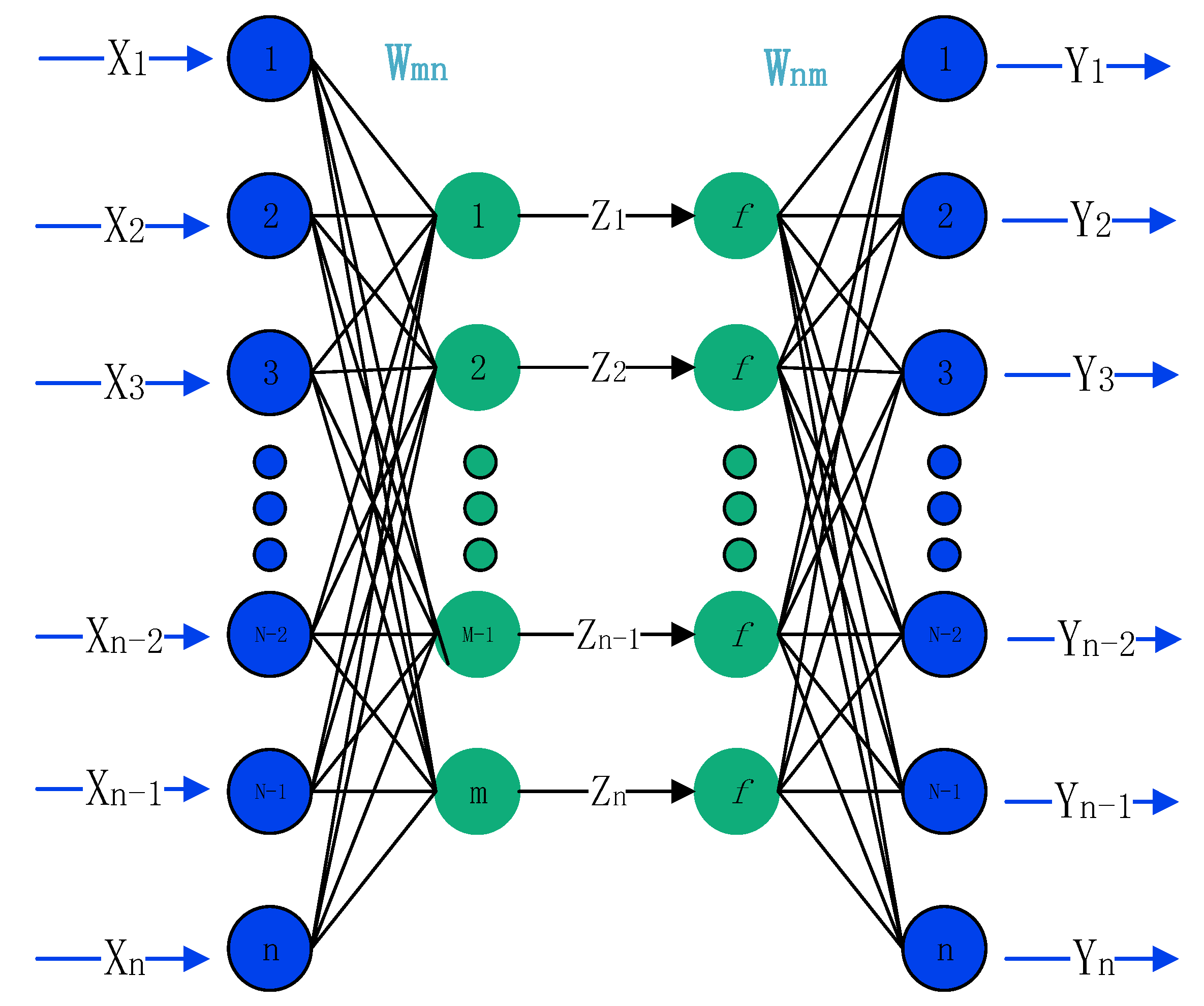
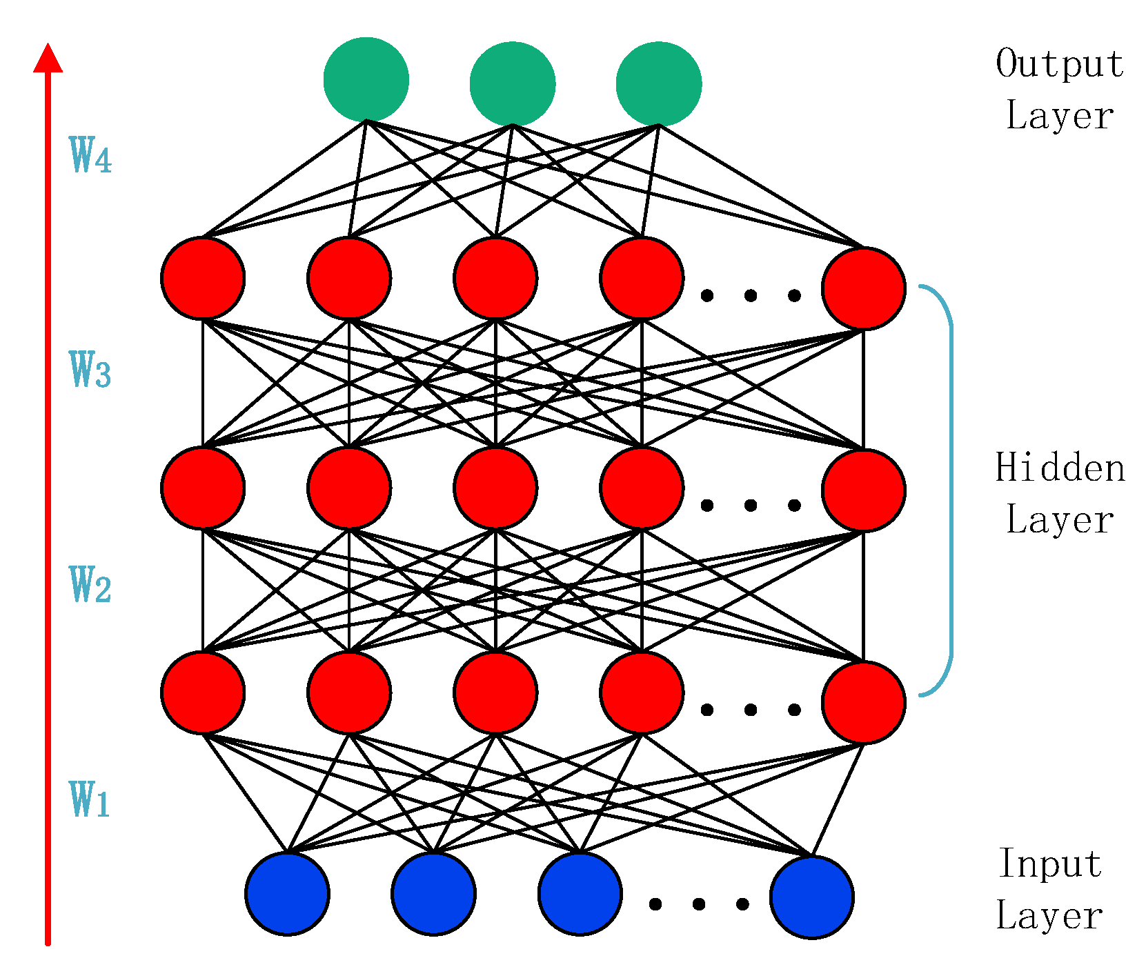
In this paper, we designed a helicopter’s sand/dust test environment. A control system for the sand and dust test environment is developed based on a reflux flow wind tunnel with a dilute gas-solid, two-phase flow field. The control system mainly uses the SAE (Stacked Autoencoder) algorithm and fuzzy controller [18]. SAE is an unsupervised algorithm consisting of a deep neural network model with multiple layers of sparse autoencoder that automatically learns features from unlabeled data and gives a better feature description than the original data [19]. The fuzzy-SAE algorithm can automatically adjust PID parameters to improve the control accuracy and speed of the sand/dust testing environment.

2. Control Scheme

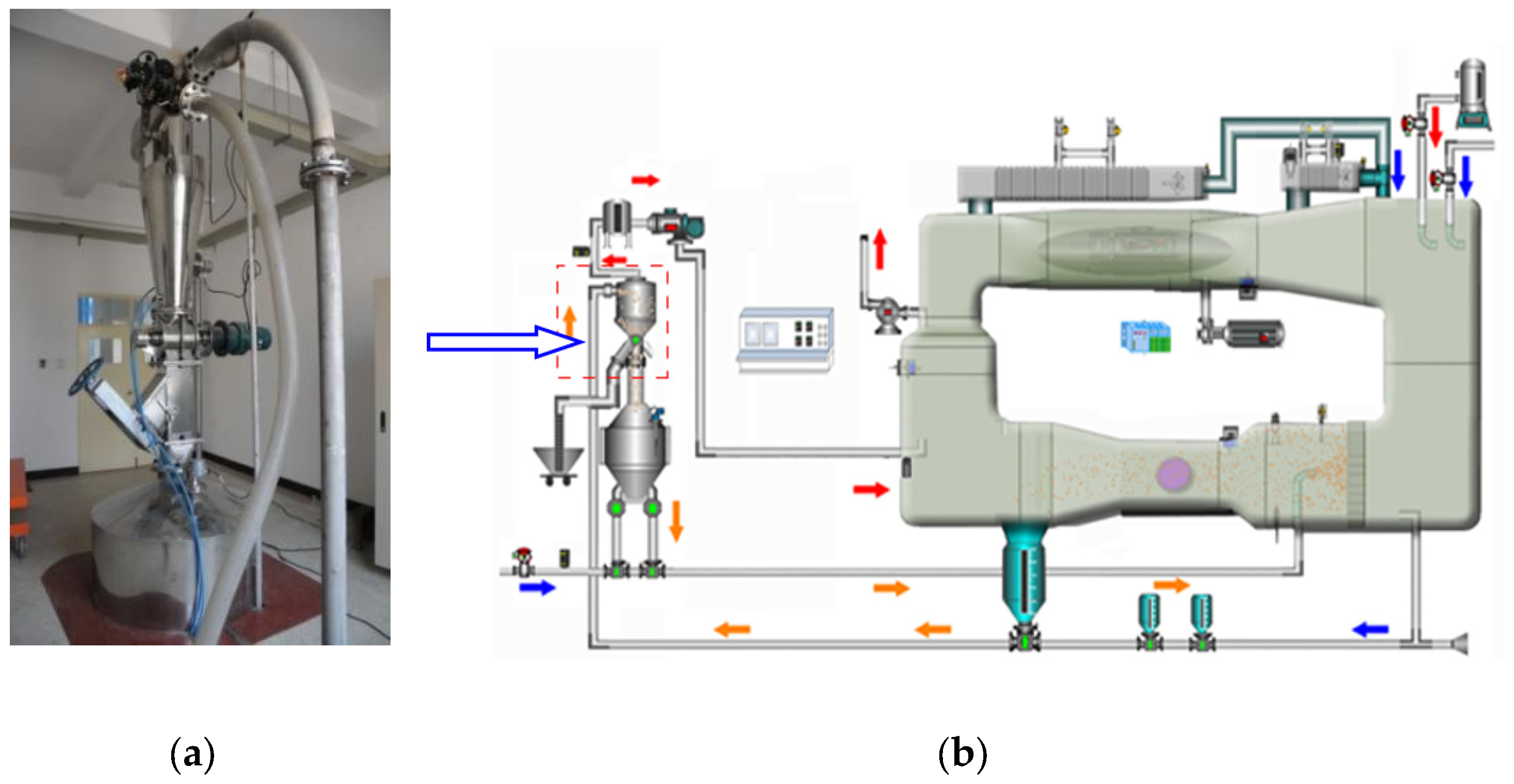
The flow chart for the pneumatic conveyance control system is shown in Figure 1. The red arrow is the flow direction of sand/dust. The blue and orange arrows are the flow directions of the cool and the hot air, respectively. The appearance of the pneumatic conveyance component is also presented in Figure 1a. 
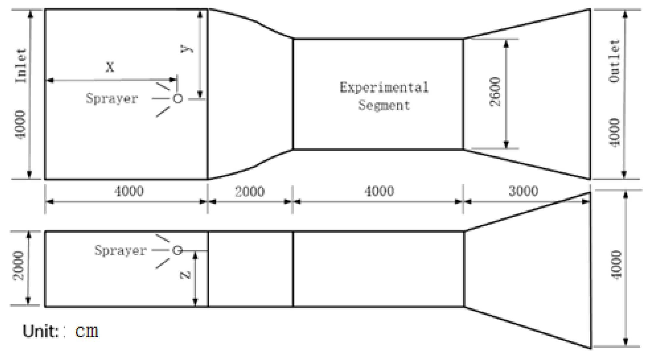
Figure 2 is a schematic diagram of the experimental wind tunnel, which is a typical wind tunnel structure.

2.1. Wind Speed Control System

The wind speed control system is based on the measurement and control system using the fuzzy controller. The wind speed can be calculated by the relationship between pressure and air density:
v = 2 ρ Δ P
where v is wind speed value, ρ is the air density, Δ P 
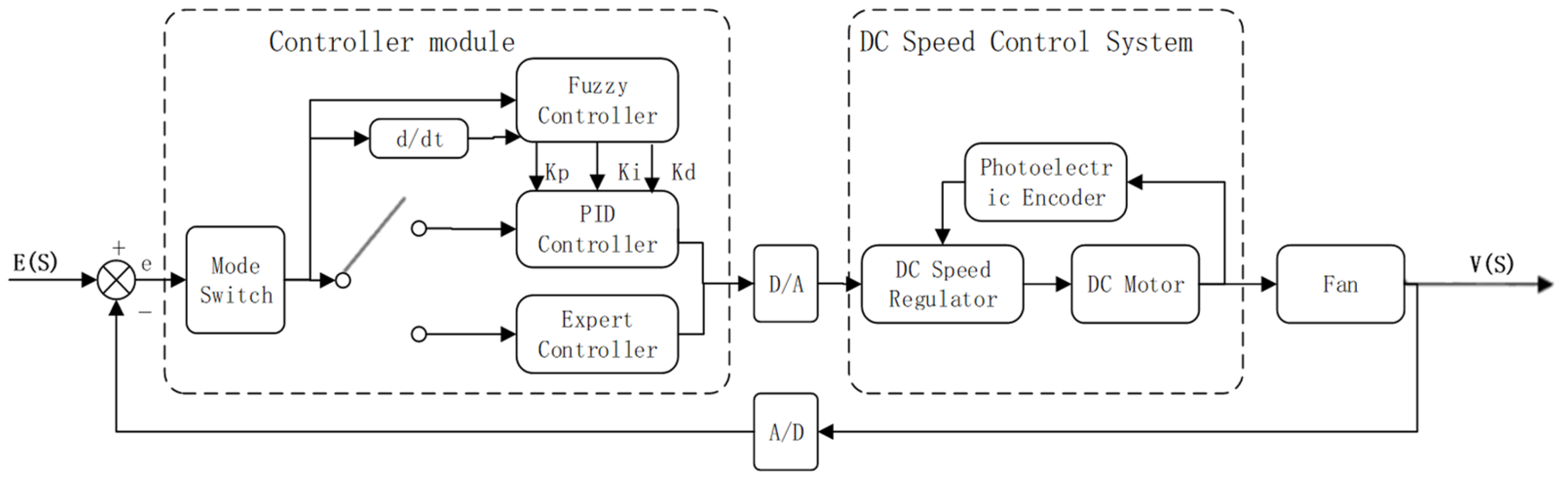
is the difference in pressure between the total pressure and the static pressure of the wind tunnel test section, and is measured by using a high-precision, differential pressure transducer that delivers measurements to the computer by a 16-bit (analogue/digital converter) acquisition. The controller is composed of a mode selection switch, a fuzzy controller, and an expert controller. The fuzzy controller consists of a fuzzy parameter regulator and a standard PID controller. The D/A (digital/analogue converter) converts a computer controlled digital value into an analogue current, that is, the standard current signal, and transports it to the governor SSR (Solid State Relay) thermostat. The DC motor power in the wind tunnel is 300 kW. The DC motor speed control system, a closed-loop speed adjustment system, is composed of a DC speed regulator, a DC motor, and a photoelectric encoder. Figure 3 shows the schematic diagram of the wind velocity measurement and control system.
In the wind speed feedback control system, the control console is the analogue comparator element using A/D to collect the data, and the D/A to produce output signals. The DC speed regulator is an actuator and the wind speed is the controlled variable, measured by the wind speed sensor.

2.2. Pneumatic Conveyance and Concentration Control System

The function of this system is to adjust the amount of sand/dust in the circulating air duct beyond the spray head. Further, it ensures that the sand/dust concentration in the control test section is in accordance with the requirements and is kept uniform along the interface.
The sand/dust concentration is measured by a sand/dust sensor transmitter that is installed on the top of the inlet duct of the test section. The input of 4 to 20 mA is a standard DC signal to the controller. Next, the controller operation produces a 4–20 mA output control signal. Adjustment of the rotary feeder speed is performed by a frequency converter, R4. This changes the amount of sand/dust and keep the concentration of sand/dust at the set value [20].
The concentration uniformity is related to the shape, quantity, arrangement, spraying angle, and length of the nozzle. In light of our analysis, we determined that the use of two or three nozzles is sufficient. The nozzle shape can be chosen to have a circular straight channel, or circular expansion, or square expansion. The injection angle, the number of nozzles, and the shape were chosen based on an experiment carried out in the open wind tunnel by the Cold and Arid Regions Research Institute of the Academy of Sciences [4]. The distance from the nozzle to the test section was also determined from that experiment.
The average value of the three sand/dust sensors’ transmitted signal is used as the control signal. We used the EMP7-3270 dust concentration online monitor (Australian Plateau Corporation, Sydney, Australia), which is manufactured by the Australian Plateau Corporation (GOYEN). The technical index of the device is shown in Table 1.
After a blowing sand/dust test, especially the duct test, sand and large dust material will be recycled into the material storage barrel after settlement and separation. However, the suspended dust in the circulating air flow must be cleared otherwise it may impact the ratio of sand and dust in the next test.

2.3. Hardware Design

The main air duct is a reflux type, low speed wind tunnel. The sand/dust recycling system consists of the recovery system, the feeding system, the electric control system, and the fixed supporting and grounding equipment. The concentration of sand/dust is different in the two working conditions, ranging from 0.1–20 g/m3. The concentration of sand/dust is controlled by the rotation of the material valve through the frequency converter. The experiment used the Mitsubishi E500 inverter (Tokyo, Japan). The control of the sand/dust concentration must be carried out under a certain wind speed. The same sand/dust concentration will change at different wind speeds with a constant sand/dust feed amount. This experiment selected the EMP7 smoke emission monitor (Australian Plateau Corporation, Sydney, Australia) for the sand/dust concentration measurement. The dust particles flowing through the probe generate an electric charge that measures the online dust emissions (unit = mg/sec or g/h). Given a constant velocity, the corresponding emission concentration (mg/m3) can be determined accurately as a function of the velocity of the smoke and dust.
This experiment adopts the PID automatic control scheme of negative feedback. The concentration sensor is the measuring element. The console data acquisition and output value comparison is the comparing element. The rotary valve feeder that controls the sand/dust amount is the controlled object. The dust concentration is the controlled variable, and a change of the wind speed is a disturbance of the concentration. As the executive component, the frequency converter motor controls the rotary feed valve. 
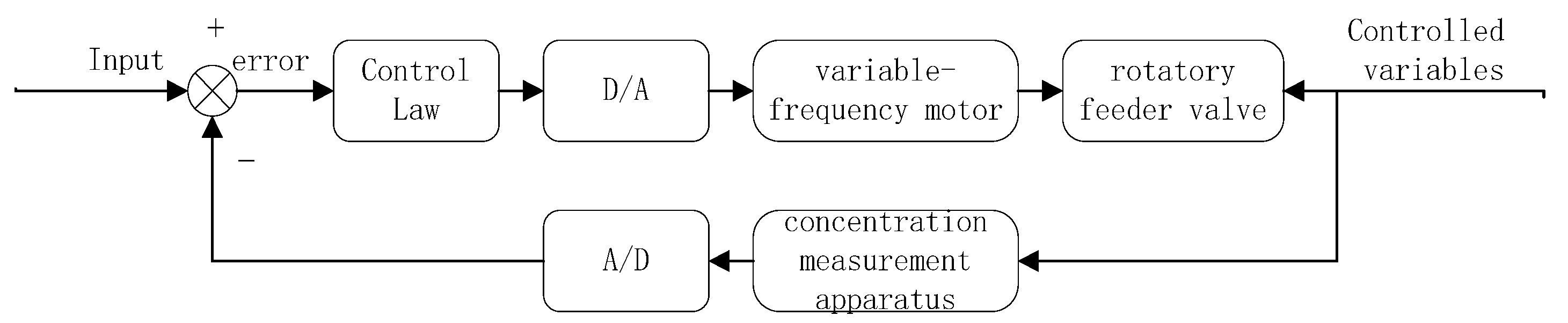
Figure 3 shows the flow chart of the control system. Figure 4 is the dust concentration feedback control block diagram.
In the feedback control system for the wind speed, the control panel is the comparison component, which collects data through the A/D and outputs an analogue quantity through the D/A. The DC speed control system is the implementation component, the wind speed is the controlled variable, and the wind speed sensor is the measuring element. The main air duct is a low speed closed circuit wind tunnel. The sand/dust recycling system includes the recovery system, the feeding system, the electric control system, and fixed supporting and grounding equipment.
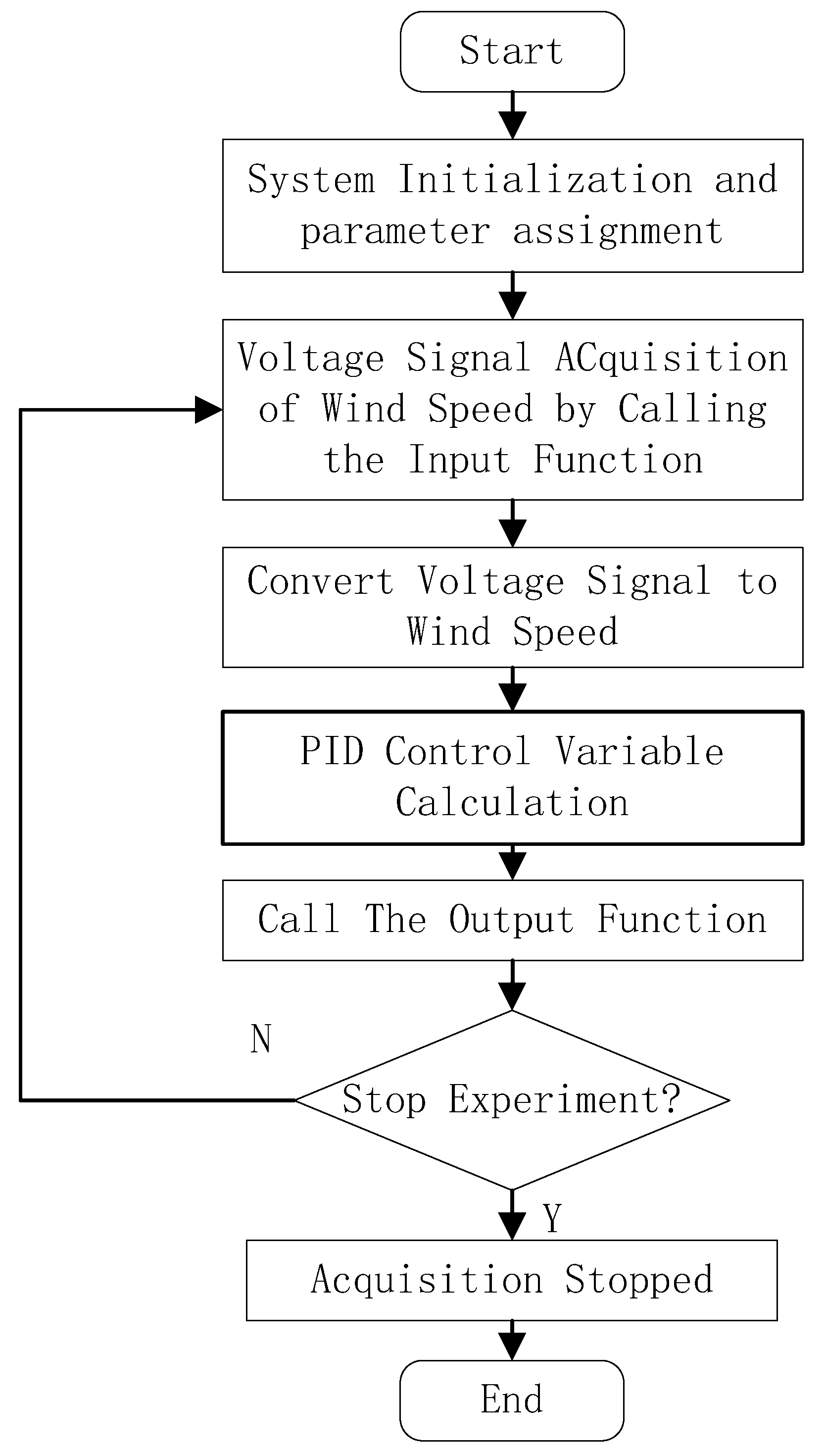
Consider the wind speed parameter as an example. Our experiment involved writing the procedure in the dialog box, adding the hardware drive function, and designing the computer data acquisition and control program—where T is the sampling period in seconds. The flow chart of such a program is shown in Figure 5.

2.4. PID Control Algorithm

We first introduce the vocabulary of the PID control algorithm [21]. The algorithm primarily uses the following formulas [22]:
u ( t ) = K p e ( t ) + 1 T i 0 t e ( τ ) d τ + T d d e ( t ) d t
Next, the program will be implemented according to:
u ( n ) = u ( n 1 ) + K p [ e ( n ) e ( n 1 ) ] + K i e ( n ) + k d [ e ( n ) 2 e ( n 1 ) + e ( n 2 ) ]
where u ( n ) is the nth output, e ( n ) is the sampling bias, K i = K p T T i is the integral coefficient, T i is the integration time constant, K p is the proportional coefficient, K d = K p T d T is the differential coefficient, T is the sampling period and T d is the differential time constant [23].
The temperature should be controlled to stay in the range of 20 to 60 °C. The task of temperature control is accomplished by both the temperature control system and the circulating air duct insulation structure. The polyurethane foam plastic insulation layer is 50 mm thick. An external thermal insulation structure is adopted because of the special characteristics of the device. The insulation prevents a large heat scatter into the test hall when the air temperature is higher than the ambient temperature. This reduces the energy consumption of the air conditioner when the air temperature is lower than the ambient temperature. As the equipment works, the main fan and the air conditioner driving power are ultimately converted into heat that can be quite significant. Therefore, to maintain the set temperature, the area must be cooled. In high temperature conditions, especially accompanied by low wind speed, the power driving the fan is reduced, but the heat capacity of the circulating air duct is very large due to the external heat insulation structure. In order to shorten the heating time, an electric heater is also present in the air conditioner box. The heater has another effect, namely, adjusting the temperature precisely; this makes the refrigerator conditions relatively stable and the temperature control precision higher.
The temperature control system is composed of the air conditioning box, the water chilling device, the three way regulating valve of chilled water, the frequency converter for the air conditioner fan and the corresponding equipment for measurement and control. The temperature sensor is installed in front of the feeding nozzle. The temperature controlling components include: the outlet water temperature control of the water chilling unit, the bypass control of the water quantity in the table cooler through the gas (or electric) three way regulating valve QF4, and the frequency conversion speed controlled by the combined air conditioning fan and electric heater control. In order to ensure that the chilling unit and the air conditioner maintain a stable environment and reduce the temperature induced fluctuations in the other systems, it is common to use the first three temperature control methods for the remote control. In this experiment, we set the electric heater in automatic fine adjustment working mode, and positioned the electric air valve at the inlet of the air conditioning box.
Due to the airflow carrying dust entering the air-conditioner, the dust can accumulate in the tube and fin tube of the heat exchanger, which can affect the heat transfer. Therefore, the cooling fin tube and the electric heating fin tube cannot be have the conventional fin tubes spacing; instead, the tubes should be larger and slightly higher than the norm. Accordingly, as the effective heat transfer area decreases and the fouling resistance increases, the total length of the finned tube will increase and the size of the cooling device and the electric heater will be increased. In addition, the pipeline blowing off compressed air should also be appropriately arranged so as to automatically swipe off the dust on the surface of the finned tube by the control program. Temperature measuring points are arranged on the inlet pipe of the cold water surface cooler and the bypass mixing pipe to monitor the temperature change after combining the air from the outlet of the air conditioner, outlet of the main fan, and the main fan.

3. Mathematical Models of Control System

The mathematical model is not only used for simulation. It is also used to adjust the automatic tuning parameters in real experiments. The data collected by the sensors such as temperature and wind speed are fed into the mathematical model and are able to derive the theoretically required adjustment amount, which is then input into the fuzzy-SAE controller.

3.1. The Model of Concentration

The dynamic control equation depends on the change in the sand/dust concentration in the return flow type test environment. The equation is expressed as:
[ V t s + ( 1 η t ) V t f ] d C t d t = k p μ p m p 1 + m p p p p t [ g 0 ( 1 η t ) + A t v t η t ] C t 2 Ω u 2
M p d m p d t = k f n f k p μ p m p 1 + m p p p p t
V t s is the volume in the high concentration region between the circulating air duct feeding port and separated section outlet. V t f is the total volume of the other sections. k p is the flow coefficient of the feeding tube. C t is the concentration in the test section. p t is the pressure of the circulating air duct. g 0 is the auxiliary flow rate of the circulating air duct. η t is the separation efficiency of the gas-solid separation device in the air duct. A t is the cross sectional area of the test wind tunnel. v t is the wind speed. m p , μ p , p p are the mass mixing ratio, the valve opening of the gas source, and the gas pressure of the sand/dust in feeding tube of pneumatic conveyance system, respectively. n f is the speed of the rotary feeder. Finally, M p is the air quality in the duct.
The change in concentration over time can be obtained by the law of conservation of mass.
V t d C t d t = G p t G t s G t o
V t is the converted volume considering the different concentrations of each component. G p t is the sand/dust quality in the air duct of the pneumatic conveyance system in one unit of time. G t s is the quality of the sand/dust separated in one unit of time. G t o is the sand/dust quality flowing away with the auxiliary air from the circulating air duct in one unit of time. C t is the concentration of test section.
The mixing ratio of the pneumatic conveyance system changes is described by Formula (7).
M p d m p d t = G f G p t
G f is the sand/dust flow into the pneumatic conveyance system by a rotary feeder in one unit of time.
The speed of the rotary feeder n f using the classical PID control method can be calculated by the principle of closed-loop control.
n f = K u p ( C t C t ) + K u i ( C t C t ) d t + K n d d d t ( C t C t )
The control equation of the valve opening of the pneumatic conveyance system is:
u p = K u p ( u p u p ) + K u i ( u p u p ) d t
where K u p , K u i , K n d are, respectively, the proportion coefficient, the integral coefficient, and the differential coefficient of the rotary feeder speed controller. C t and C t are, respectively, the measured value and the given value of the sand/dust concentration.

3.2. The Model of Pressure

The dynamic equation of the changing pressure is:
d P d t = C j s k j s P j s P + C t s k t s P t s P C x l C z h n z 2 P 0 C t y n t
where C j s is the sand flow factor, C t s is the moisture transfer factor, C x l is the leakage factor, C t y is the pressure regulating factor, and C z h is the main fan factor. P j s , k j s are, respectively, the pressure and the valve opening of the gas-solid two-phase flow when adding sand. If the speed of the regulating fan is selected to be the control variable, the control equation is:
n t = K p ( p s p ) + K I 0 t ( P s P ) d t

3.3. The Model of Temperature

The dynamic equation of the temperature variation in the circulating air duct is shown in Formula (12).
M t c t d θ t d t = k h n f 3 + G a c a ( θ a θ t ) k s F s ( θ t θ s ) + Q d G w c w ( θ t + Δ θ w o θ w i )
M t is the equivalent metal mass of the circulating air duct. c t is the ratio of the specific heat. θ t is the temperature of the duct. Q d is the heating power of the electric heater. n f is the speed of the fan. k h is the ratio coefficient. c a is the specific heat of the air flow. θ a is the temperature of the air flowing into the duct.
k s , F s and θ s are, respectively, the heat dissipation coefficient, the heat dissipation area, and the ambient temperature of the outer surface of the circulating air duct. At this point, the control equation of the cooling water flow is:
G w = K c p λ c v e t + K c i ( λ c v e t ) d t + K c d λ c v de t d t
G w is the amount of cooling water. e t is the deviation signal between the test temperature and the measured value. K c p , K c i and K c d are, respectively, the proportion coefficient, the integral coefficient, and the differential coefficient of the electric heater. The control equation for the heating power of the electric heater is shown in Formula (14).
Q d = K t p ( 1 λ c v ) e t + K t i ( 1 λ c v ) e t d t + K t d ( 1 λ c v ) d e t d t
Q d is the heating power of the electric heater. K t p , K t i , K t d are, respectively, the proportion coefficient, the integral coefficient, and the differential coefficient of the electric heater.

4. Control Algorithm

4.1. Fuzzy Control Strategy for Wind Speed

As we can see from Figure 3 showing the fuzzy controller [24], the wind speed can be calculated by Formula (1) after the differential pressure sensor measures the pressure difference Δ P . By setting the wind speed to be V0 and the velocity deviation to be e, the deviation change rate Δ e can be computed. When using the e and Δ e as the inputs, expert control or fuzzy control can be chosen with the mode switch. PID control is chosen when e is greater than the setting value, while expert control is chosen when e is smaller than the setting value [25].
The output of the controller should be kept constant when the measured value of the wind speed reaches the accuracy of the experiment. In this method, the speed of the motor is constant and the wind in the circulating air duct is blown through a few cycles of the wind tunnel to stabilize. Thus, the wind speed can be achieved within the error allowed by the test requirements [26]. The expert controller depends upon expert judgment. This judgment is primarily reflected in the if-then statement in the program [27].
The fuzzy controller is based on the conventional PID controller. The fuzzy theory establishes the parameters k p , k i and k d , the absolute deviation | E | and deviation change | Δ E | . It can adjust the k p , k i and k d by itself, online, according to different | E | and | Δ E | . The general form of the control function of the conventional PID regulator is
U ( k ) = k p e ( k ) + k i e ( k ) + k d Δ e ( k )
k p , k i , k d are the ratio coefficient, the differential coefficient, and the integral coefficient, respectively. k is a value between 0 and n. e ( k ) is the deviation and Δ e ( k ) is the deviation change rate. The fuzzy adaptive PID controller design can be achieved according to the following five steps discussed in Section 4.1.1, Section 4.1.2, Section 4.1.3, Section 4.1.4 and Section 4.1.5 below.

4.1.1. Fuzzy Process

The practical range of values of e ( k ) and Δ e ( k ) is [−60, 60] and 60 is the maximum opening wind speed. We transform e ( k ) and Δ e ( k ) into a more precise domain in order to realize the fuzzy control method’s coarse tuning and fine tuning.
| e | = ln | e ( k ) | 3 | e ( k ) | > 3 0 3 e ( k ) 3
| Δ e | = ln | Δ e ( k ) | 3 | e ( k ) | > 3 0 3 e ( k ) 3
This process of dynamic range is greatly compressed after the transformation.We then turn them into two fuzzy variables. Both contain fuzzy sets {NB, NM, NS, Z, PS, PM, PB}. NB represents negative big, NM represents negative medium, NS represents negative small, Z represents zero, PS represents positive small, PM represents the positive median, and PB represents positive big. The membership functions of linguistic variable E and Δ E can select linear or nonlinear functions according to the actual situation. The mathematical forms of their membership functions are as follows.
μ B E = 1 | E | > | E | 3 | E | | E | 2 | E 3 | | E | 2 | E | 2 | E | | E | 3 0 | E | < | E | 2
μ M E = 0 | E | < | E | 1 | E | | E | 1 | E | 2 | E | 1 | E | 1 | E | | E | 2 | E | 3 | E | | E | 3 | E | 2 | E | 2 | E | | E | 3 0 | E | > | E | 3
μ S E = 1 | E | < | E | 1 | E | | E | 1 | E | 2 | E | 1 | E | 1 | E | | E | 2 0 | E | > | E | 2
μ B Δ E = 1 | Δ E | > | Δ E | 3 | Δ E | | Δ E | 2 | Δ E 3 | | Δ E | 2 | Δ E | 2 | Δ E | | Δ E | 3 0 | Δ E | < | Δ E | 2
μ M Δ E = 0 | Δ E | < | Δ E | 1 | Δ E | | Δ E | 1 | Δ E | 2 | Δ E | 1 | Δ E | 1 | Δ E | | Δ E | 2 | Δ E | 3 | Δ E | | Δ E | 3 | Δ E | 2 | Δ E | 2 | Δ E | | Δ E | 3 0 | Δ E | > | Δ E | 3
μ S Δ E = 1 | Δ E | < | Δ E | 1 | Δ E | | Δ E | 1 | Δ E | 2 | Δ E | 1 | Δ E | 1 | Δ E | | Δ E | 2 0 | Δ E | > | Δ E | 2
The membership function curves of E and Δ E are shown in Figure 6.

4.1.2. Establishing Rules of Inference

The fuzzy rules of k p , k i and k d for the control system are established as follows:

4.1.3. Fuzzy Inference and Defuzzification

According to the system sampling of E and Δ E , the parameters of the controller can be calculated by Formula (24).
The relationship in every part is “and”, so the AND operation is used. The value of the membership of antecedent can be expressed as μ j which is shown in Formula (25).
k p = j = 1 9 μ j ( E , Δ E ) k p j j = 1 9 μ j ( E , Δ E ) k I = j = 1 9 μ j ( E , Δ E ) k I j j = 1 9 μ j ( E , Δ E ) k d = j = 1 9 μ j ( E , Δ E ) k d j j = 1 9 μ j ( E , Δ E )
μ j ( | E | , | Δ E | ) = μ j ( | E | ) μ j ( | Δ E | )

4.1.4. Parameter Acquisition

When the error | E | is large, in order to ensure that the system has a good speed tracking performance, k p ought to be larger and k d ought to be smaller, regardless of the variation tendency of the error. At the same time, a smaller k i value avoids a large over-shoot in the system response. When the error in E is of a medium size, k p should be a smaller value to keep a smaller overshoot in the system response. At the same time, to ensure the system’s response speed is sufficient, k i and k d should be moderate in size. The value of k d has a significant influence on the system response. When the error in E is small, kp and ki should be greater values. The fuzzy inference rules of k p , k i , k d are shown in Table 2.

4.1.5. Adding Expert Judgment

When the value of the measured wind velocity is in the vicinity of the set value and the required accuracy is achieved, the mode selection switch should switch to the expert control state. The output of the controller holds the line, meaning u (k) = u (k − 1). This property allows the measured value to stabilize. When the measured value exceeds the steady error accuracy range, then the system is switched to the adaptive PID controller state.

4.2. Tracking Strategy by Stacked Autoencoder Neural Network

The PID control needs to adjust the coefficient ratio, the integral coefficient, and the differential coefficient into a proper state, forming a relationship of mutual coordination and mutual restraint to achieve a better control effect. Generally, the relationship between k p , k i , k d is usually nonlinear, and finding the best k p , k i , k d is a big problem. For this reason, this article uses a stacked autoencoder composed of a multilayer neural network, which can express any nonlinear relation. However, it is easy to fall into local extreme points in the process of training, and there is also the gradient diffusion problem in the traditional multilayer neural network. Therefore, a stacked autoencoder neural network is used in this article. We apply the layer-by-layer greedy training method, training only one layer at a time. First, a network with only one hidden layer is trained. Training the second hidden layer of the network occurs only after the completed training of the first hidden layer network, and so on. In this way, we can avoid the local extreme point problem and the gradient dispersion problem of the traditional multilayer neural network. The stacked autoencoder used in this article is composed of several autoencoders, in which the output of the former autoencoder is the input of the next auto encoder.

4.2.1. Autoencoders

Every autoencoder is composed of an input layer, a hidden layer, and an output layer. The layers are all connected between the neurons of two adjacent layers. However, there is no connection between the neurons of the same layer. As shown in Figure 7, there are n nodes of the input layer and m nodes of the hidden layer. The offset of the ith node of the hidden layer is the connection weights from the jth node of the input layer to the ith node of the hidden layer, which are the connection weights from the ith node of the hidden layer to the jth node of the output layer, and so on. The input is [ x 1 , x 2 , , x n ] T and the output is [ y 1 , y 2 , , y n ] T . The autoencoder consists of two parts, encoding and decoding.
Encoding: The weight matrix W i j is randomly initialized and calculates the activation value of the hidden layer neurons by Formula (26), which is here noted as [ O 1 , O 2 , , O m ] T .
o 1 o 2 o m = w 11 w 12 w 1 n w 21 w 22 w 2 n w m 1 w m 2 w m n x 1 x 2 x n + b 1 b 2 b m
Decoding: The nodes of the output layer are the same as the input layer. The weight matrix W j i is randomly initialized and calculates the activation value of the output layer neurons by Formula (27).
y 1 y 2 y n = w 11 w 12 w 1 m w 21 w 22 w 2 m w m 1 w m 2 w n m o 1 o 2 o n + b 1 b 2 b n
The cost function is shown in Formula (28).
J = 1 2 i = 1 n ( y i x i ) 2
Finally, the algorithm uses the gradient descent method and gets the final W i j and b i that make the cost function converge. The terms of interest [ O 1 , O 2 , , O m ] T are calculated using W i j and b i .

4.2.2. Stacked Autoencoder

In this article, a stacked autoencoder with five layers is used that includes three autoencoders—that is, the network contains one input layer, one output layer, and three hidden layers. The topological graph of the stacked autoencoder is shown in Figure 8.
The input layer is:
O j ( 1 ) = x ( j ) ( j = 1 , 2 , , M )
The output layer contains three neurons corresponding to the three adjustable parameters k p , k i , k d . A non-negative sigmoid function is chosen because k p , k i , k d cannot be negative. The basic training process of the stacked autoencoder is as follows:
  • Using multiple auto encoders to construct the neural network and using the sample as the input;
  • Training the network layer by layer: transform the data into the reconstruction data by encoding and decoding; calculate the cost function, minimize it, and compute the optimal { W m n , b n } , which is the initial weight for the neural network;
  • Train each autoencoder in turn according to the steps in (b) and record the { W m n , b n } generated by every autoencoder: complete the training of the entire deep neural network and realize the PID adaptive adjustment control;
  • Use “random gradient Descent”.
By contrast to using standard gradient descent to calculate the gradient accurately, the stochastic gradient descent method adds random factors to calculate the gradient, so even if it falls into the local minimum point, the gradient it calculates may still not be 0, and it is therefore possible to jump out of the local minimum and continue searching.

5. Simulation

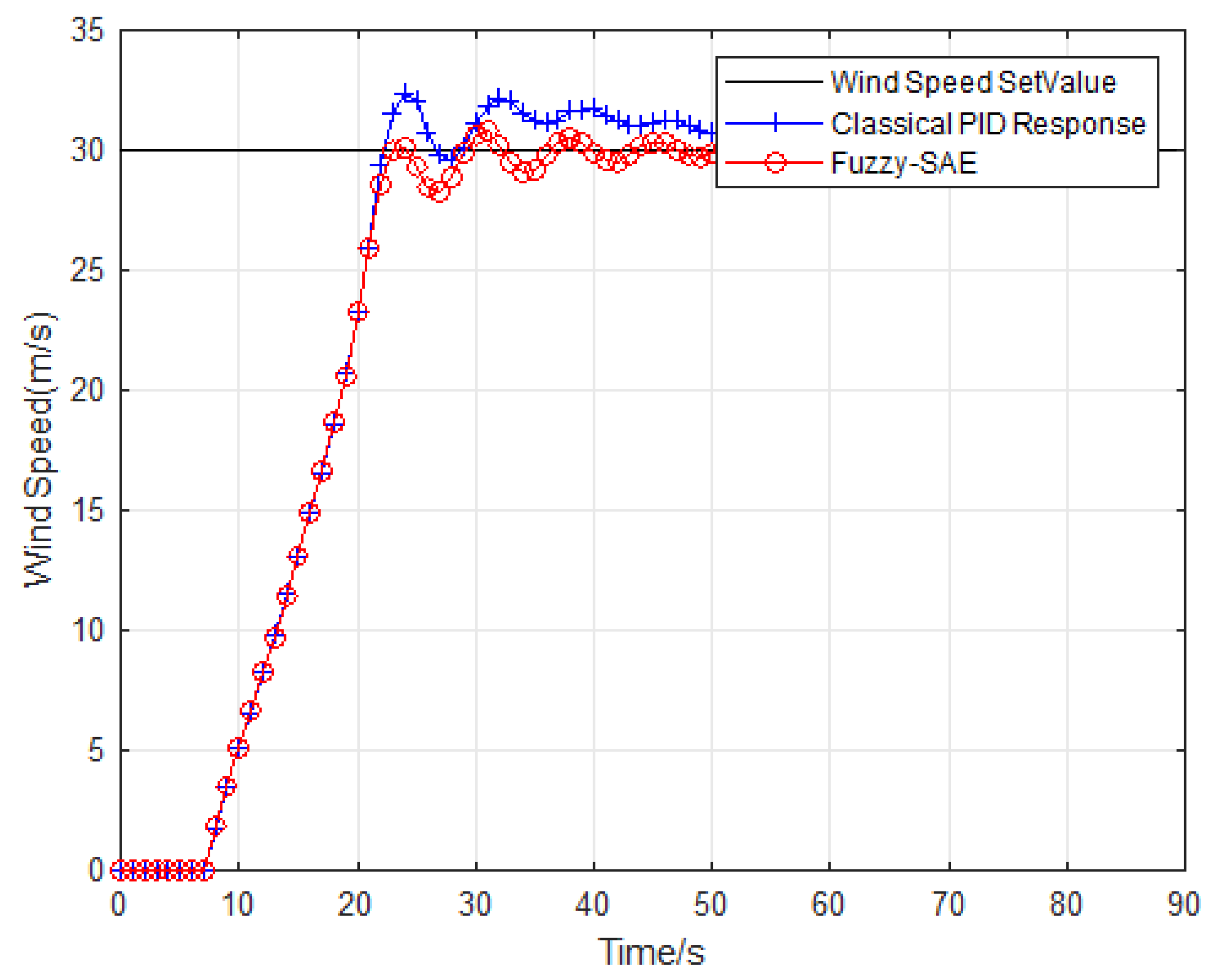
To initially verify the effectiveness of the algorithm, we observe the results of the two algorithms by simulation. Using a wind speed simulation, the fuzzy-SAE algorithm and the classic PID algorithm curve chart is shown in Figure 9.
In the simulation, the PID parameters are set through several attempts and the corresponding parameters are modified according to the control effect to finally select the best parameters.
By comparing the simulation results, we observe that the response curve of the fuzzy algorithm is smaller and that the fuzzy algorithm achieves the required wind speed control accuracy after the control system reaches the stable state.
The measured data can also prove the above conclusion. Compared with the classic PID algorithm, the fuzzy-SAE algorithm has a better dynamic response curve for the wind speed measured in the D-4 wind tunnel of Beihang University.
As shown in Figure 9, the X-line is the classic PID algorithm. The straight line is based on the fuzzy-SAE algorithm. The PID parameter can be adjusted online by itself. When the Reynolds number changes, the speed setting value and model attitude angle change too. The fuzzy-SAE algorithm does not need to manually adjust the control parameters.
It can be seen that the wind speed variation is basically the same for both control methods at the beginning, because the algorithm has already controlled the motor to reach the maximum power at this time. However, the fuzzy-SAE quickly results in converged wind speed oscillation when the wind speed approaches the target value. 
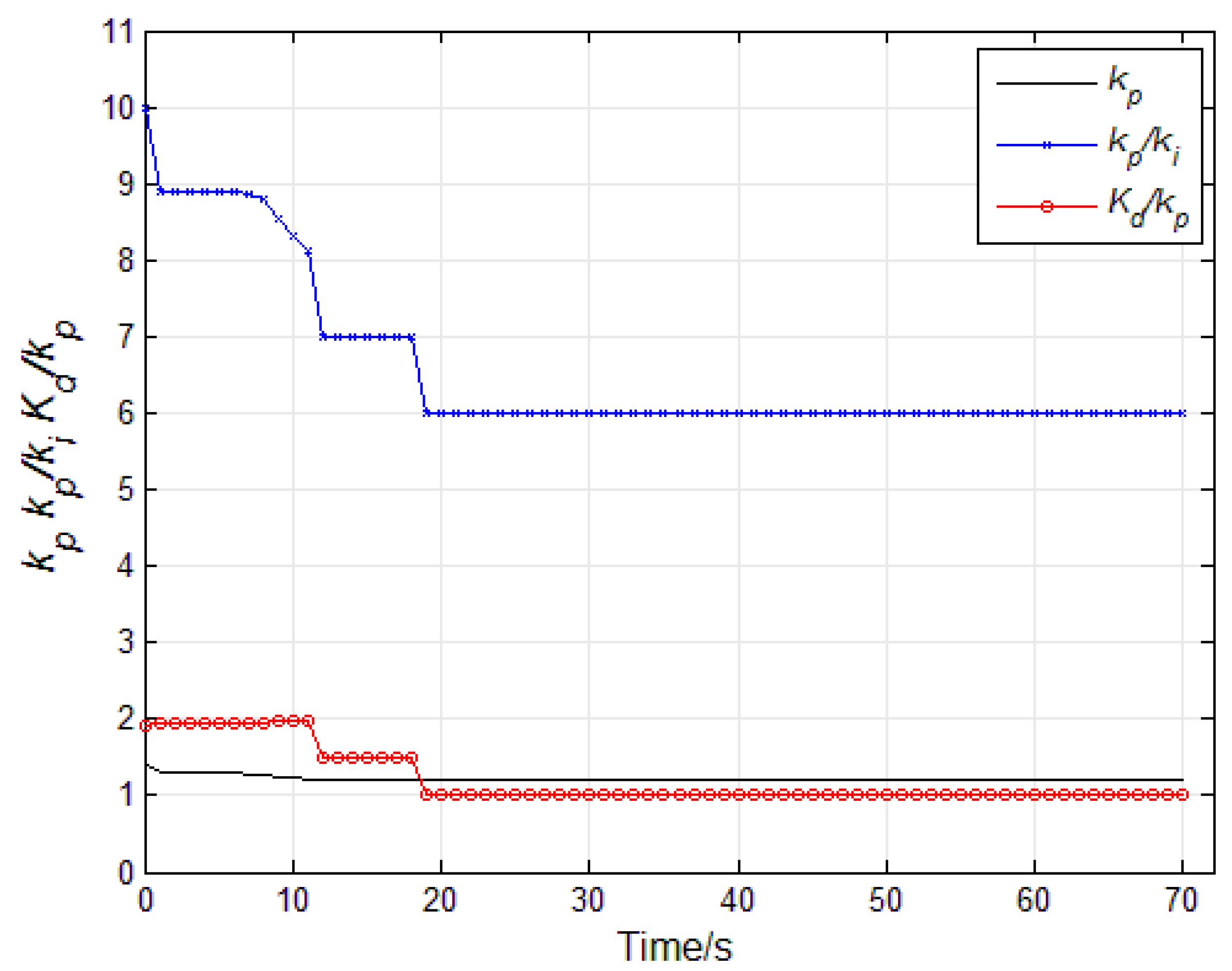
Figure 10 shows the variation of the three parameters Ki, Kp, and Kd. Due to the characteristics of the controller and the instrument itself, the three parameters are different, and Ki < Kp, and Kd > Kp. For better presentation, Kp/Ki and Kd/Kp are used to represent the parameter changes.
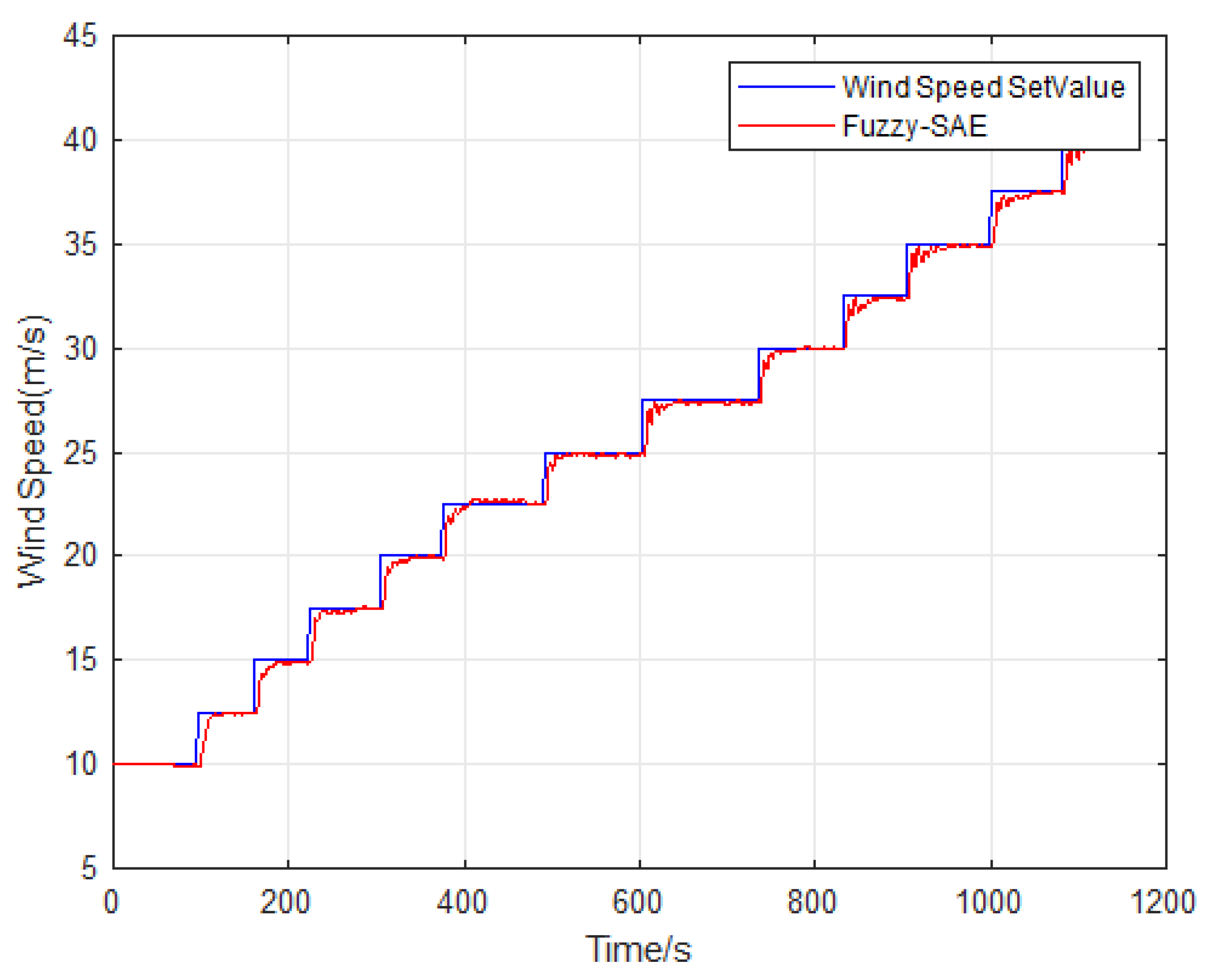
In Figure 11, the fuzzy-SAE algorithm is also able to adjust quickly without steady-state error or overshoot when the wind speed is changed.

6. Experimental Result

The experimental conditions are shown in Table 3. The requirements for these experimental environments are derived from the Chinese national standard for helicopter sand/dust testing.
In this test, blowing dust at room temperature lasts for 6 h and at a warm temperature for 6 h. The size of dust particles is less than 149 µm. The sand size is between 180 and 850 µm. All measurements were carried out in the steady state of the wind tunnel.
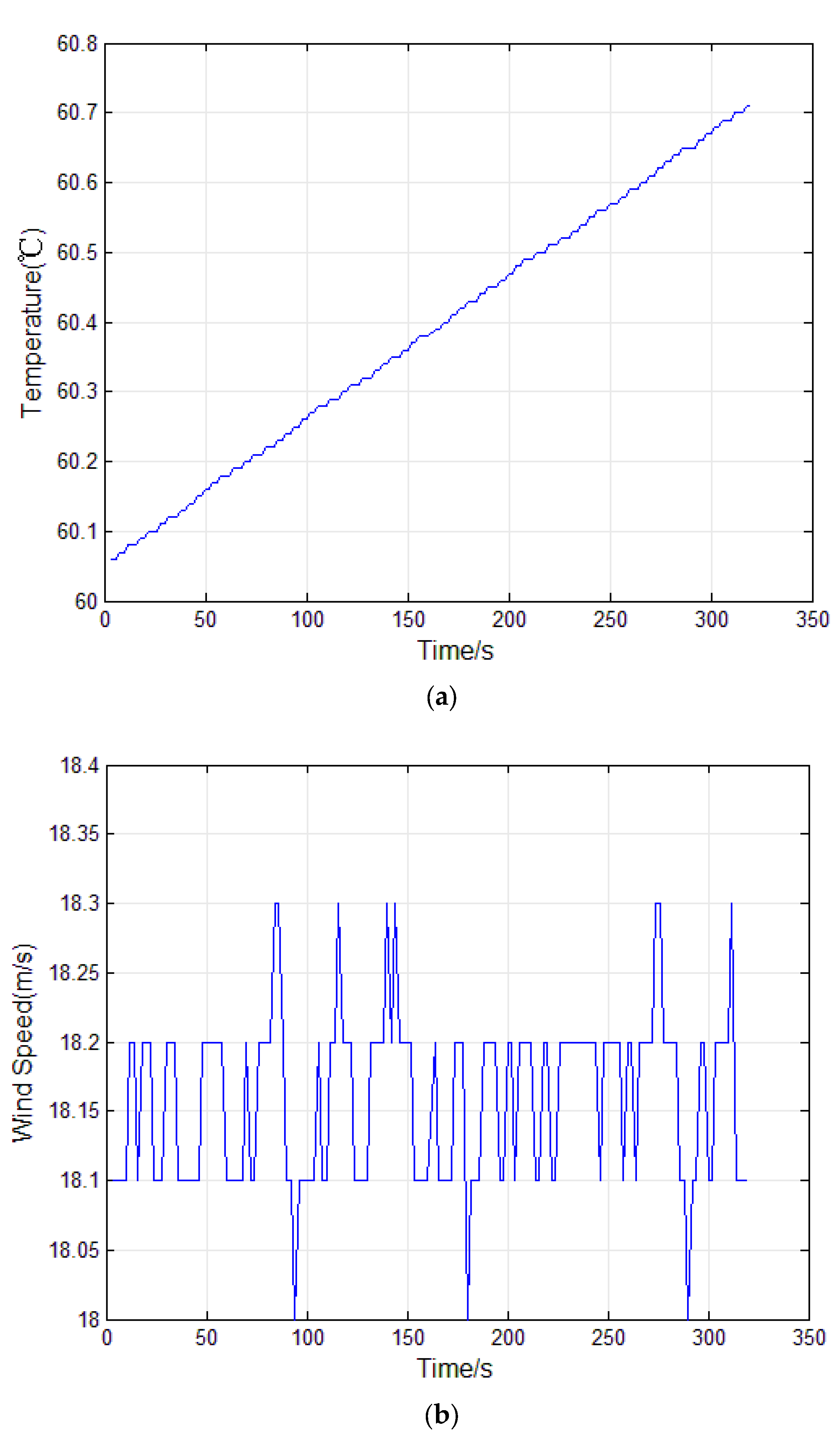
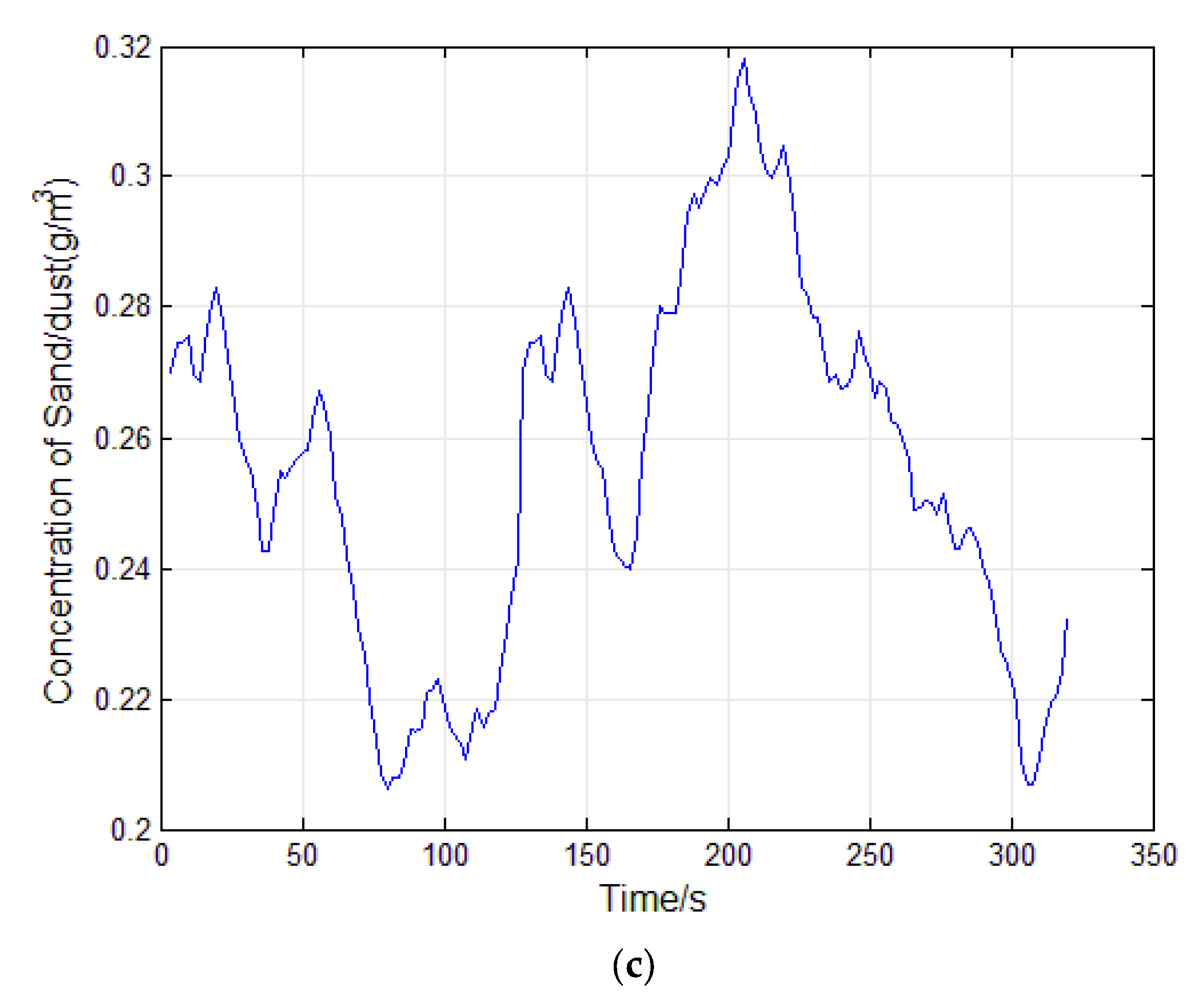
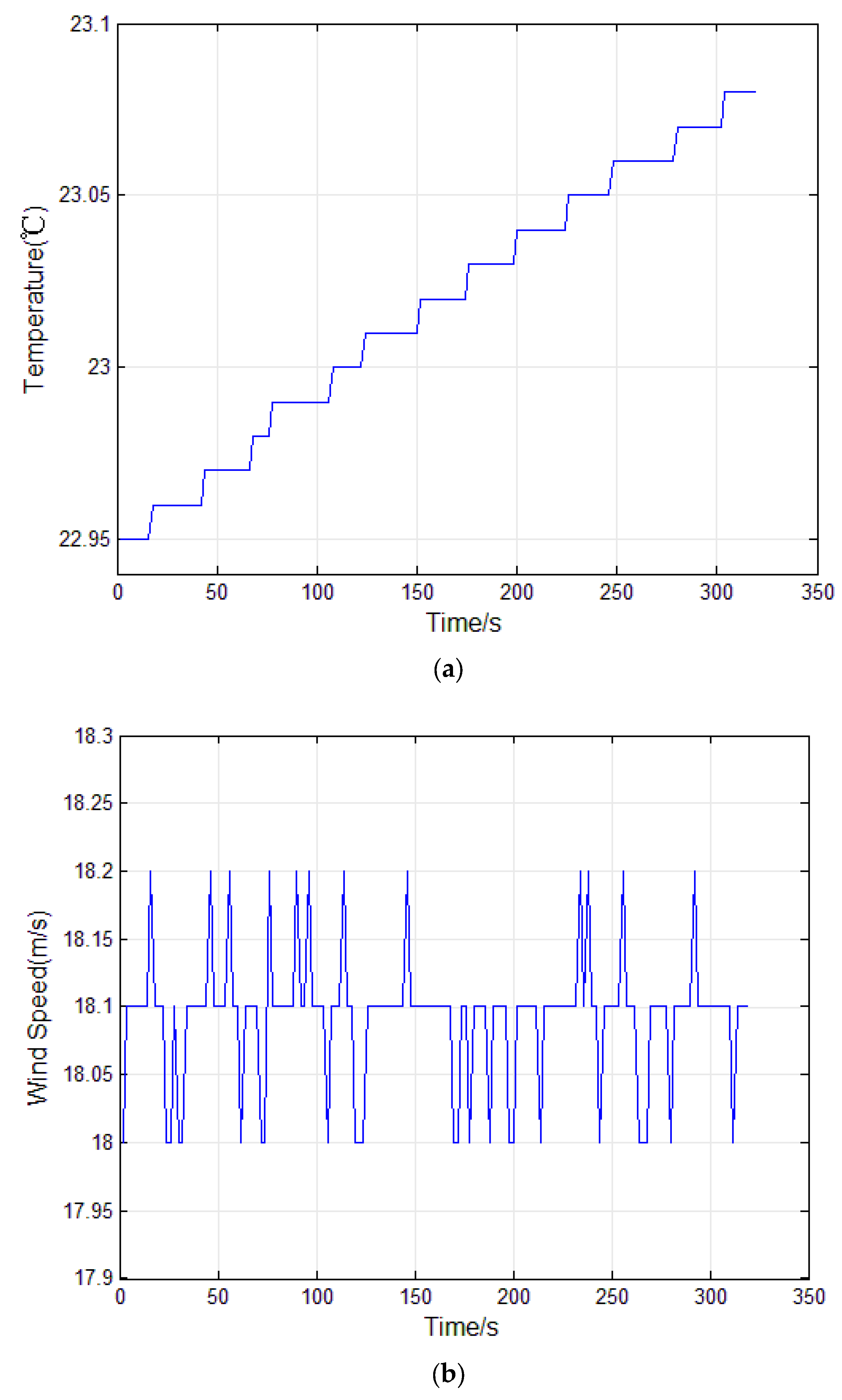
The relevant data from some test sections are as follows. The temperature, wind speed, and concentration meet the requirements of the technical specifications. Low sand concentration data are shown in Figure 12a–c. Commissioning results of 18 m/s wind speed, high temperature and low sand is shown in Table 4.
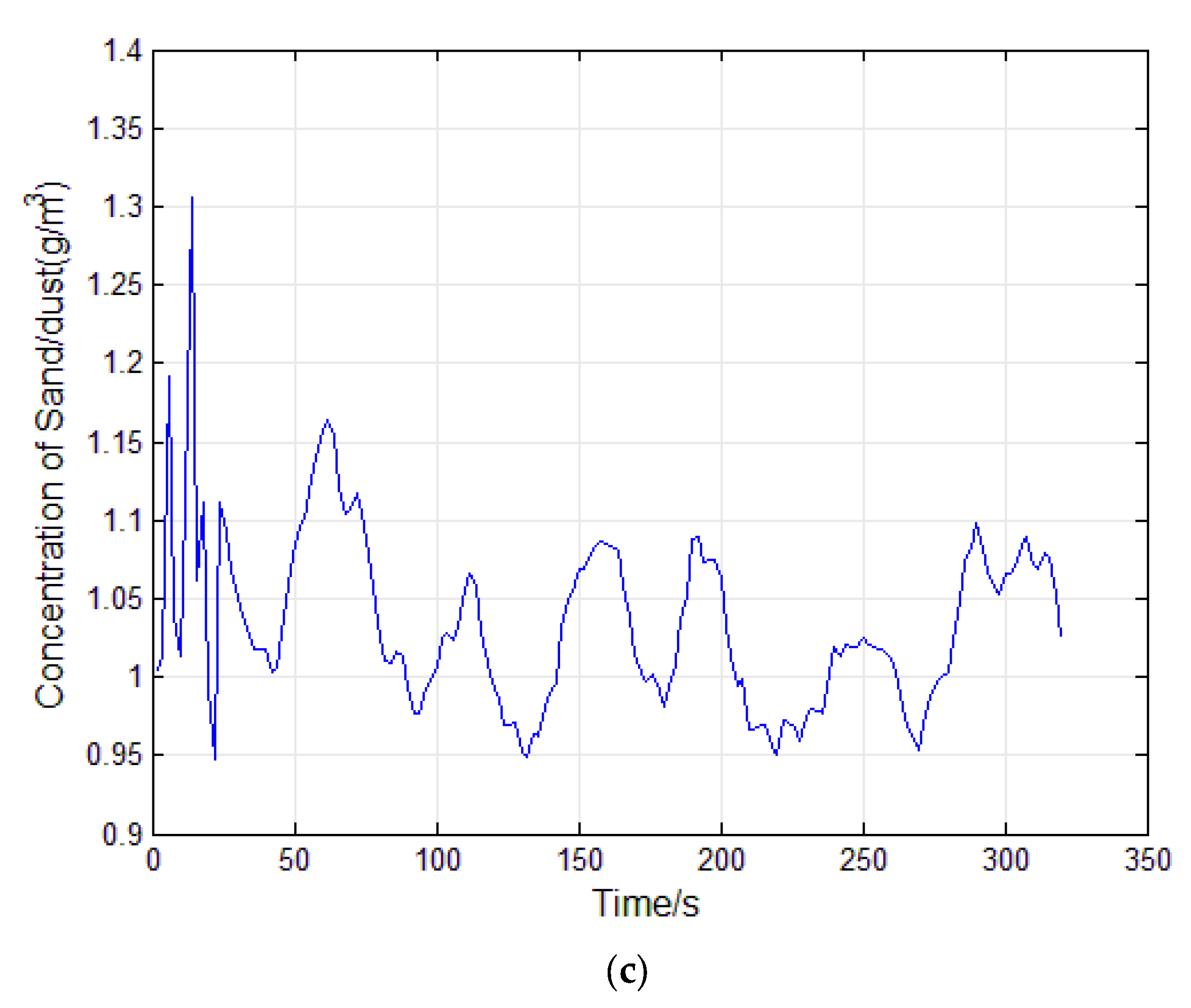
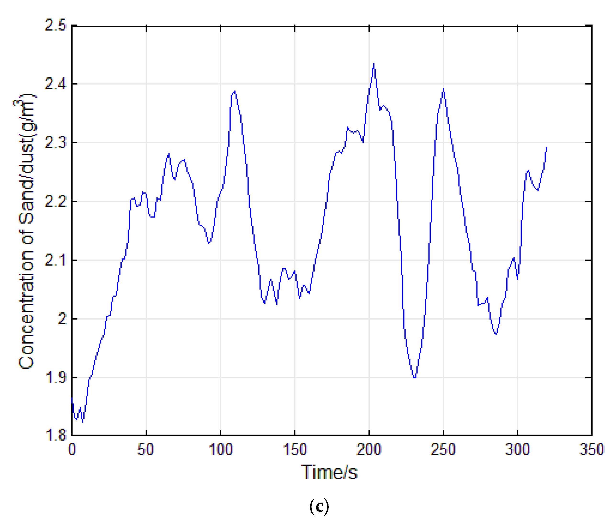
Medium sand concentration data are shown in Figure 13a–c. Especially in Figure 13c, fluctuation in the initial phase of the experiment is significant. The concentration is disturbed when suddenly adding sand and dust into the test tunnel and generally four cycles are required to achieve uniform concentration. Commissioning results of 18 m/s wind speed, high temperature and medium sand is shown in Table 5.
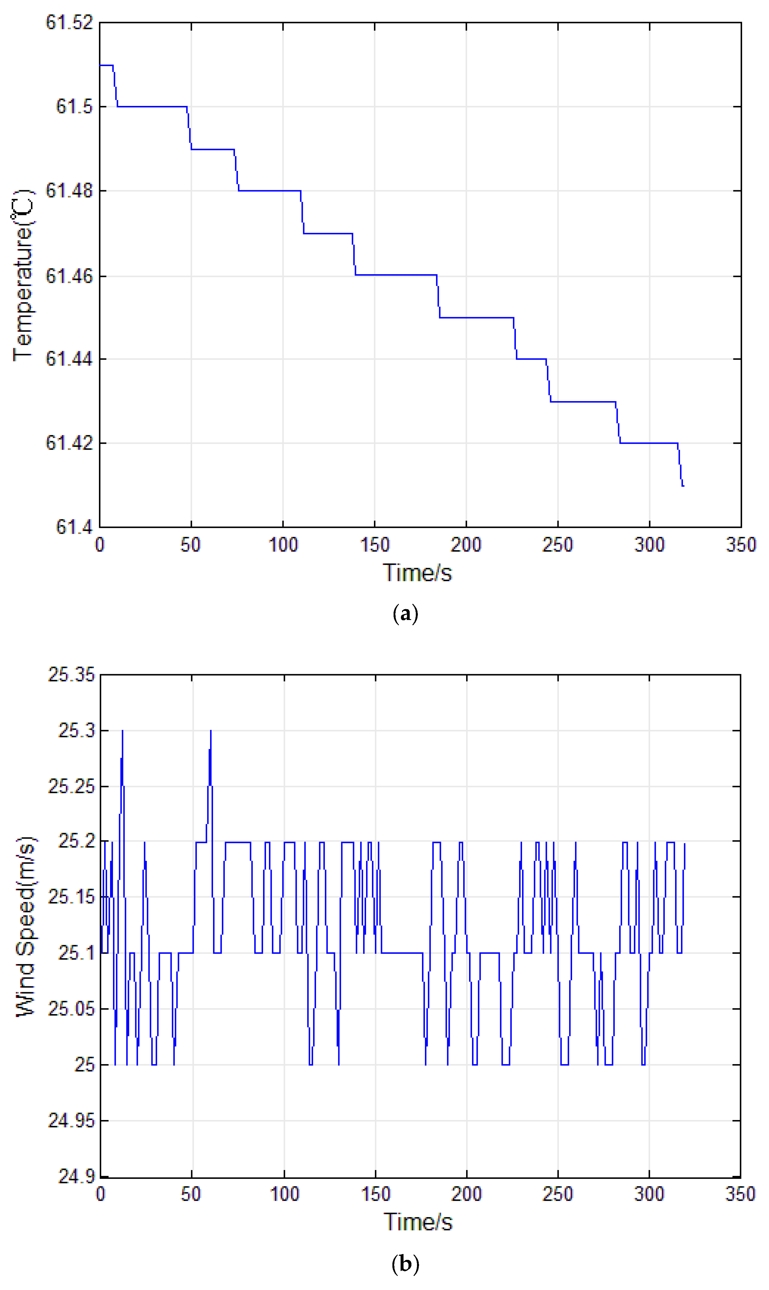
High sand concentration data are shown in Figure 14a–c.
The fluctuations of temperature and wind speed are very small. Sand/dust concentration is slightly unstable, but still meets the requirements of sand and dust test environment.
By carrying out the tests under three different working conditions, it can be seen that the fuzzy-SAE algorithm can accurately control the temperature, wind speed, and sand/dust concentration, and meets the requirements of helicopter sand/dust experiments.
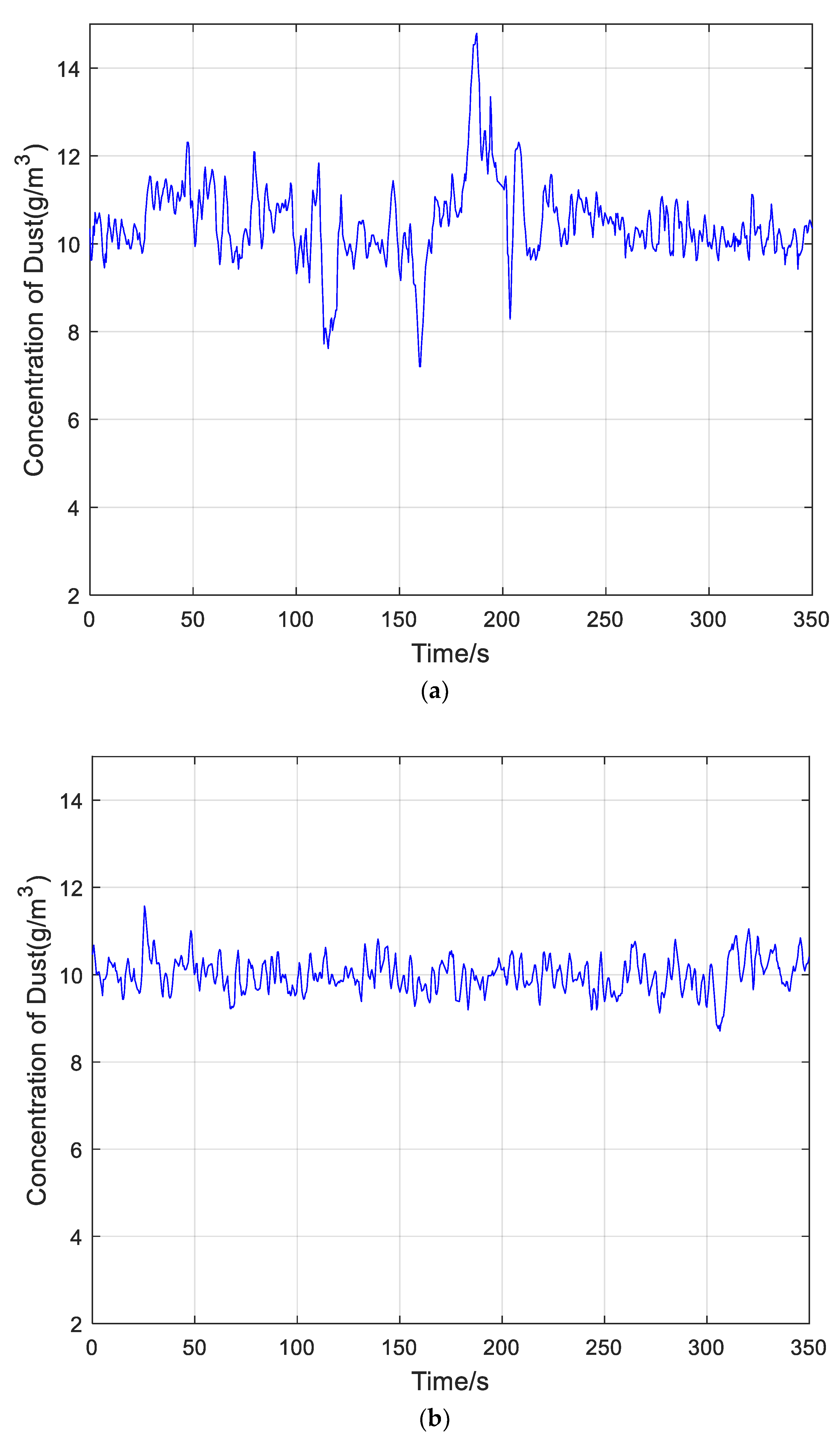
Figure 15 shows the results of the dust blowing experiment. Experiments were conducted using both fuzzy-SAE and PID controllers, at 23 °C and 8.9 m/s wind speed. The parameters of the PID controller were set in the same way as the simulation. Commissioning results of 25 m/s wind speed, high temperature and low sand is shown in Table 6.
Both algorithms can meet the 10 g ± 7 g requirement. However, it can be seen that the fuzzy-SAE controller has better smoothness, and smaller stability error. This indicates that our proposed fuzzy-SAE algorithm offers a significant improvement over the traditional PID algorithm.

7. Conclusions

A sand/dust environment is one of the most important factors that must be considered in helicopter failure. It is technologically difficult to simulate such an environment by wind tunnel, especially the temperature control, wind speed control, sand/dust concentration, and controlled particle distribution uniformity. The fuzzy intelligent control method and the deep neural network tracking strategy proposed in this paper can control the experimental parameters very well, with a smaller overshoot, faster response speed, no steady error, and a better dynamic response curve compared to the classic PID control. This method better meets the standard technical indicators with regard to the test temperature, wind speed, and sand/dust concentration in the wind tunnel. The fuzzy-SAE intelligent control method not only has the high accuracy of the classic PID control method but also has the high speed, stability, and robustness afforded by fuzzy control, which can meet the intelligent control requirements of the sand/dust environment test equipment. The design and control method has a reference value for the construction of similar sand/dust environmental wind tunnels and lays the experimental foundation for further studies.

Author Contributions

Conceptualization, K.L. and J.W.; methodology, K.L.; software, Y.L.; validation, L.M., Y.L. and M.L.; formal analysis, Y.L.; investigation, L.M.; writing, K.L. and M.L.—original draft preparation. All authors have read and agreed to the published version of the manuscript.

Funding

The authors are supported by the National Natural Science Foundation of China (No. 61773039), and the Aeronautical Science Foundation of China (No. 2017ZDXX1043 and 2018XXX).

Conflicts of Interest

The authors declare no conflict of interest.

References

  1. Zhang, Y.; Jiang, C.; Zhan, X. Modelling the multi-physics of wind-blown sand impacts on high-speed train. Wind. Struct. 2021, 32, 487. [Google Scholar]
  2. Vijayakumar, R.; Seshadri, V.; Singh, S.N.; Kulkarni, P.R. A Wind Tunnel Study on the Interaction of Hot Exhaust from the Funnel with the Superstructure of a Naval Ship. In Proceedings of the OCEANS 2008—MTS/IEEE Kobe Techno-Ocean, Kobe, Japan, 8–11 April 2008. [Google Scholar]
  3. Blasi, L.; Barbato, S.; Mattei, M. A particle swarm approach for flight path optimization in a constrained environment. Aerosp. Sci. Technol. 2013, 26, 128–137. [Google Scholar] [CrossRef]
  4. Yin, J.; Liu, H.; Wang, J.; Li, K. Control System Design of Pneumatic Conveying in Sand/Dust Environment Simulation Test. Appl. Mech. Mater. 2013, 442, 424–429. [Google Scholar] [CrossRef]
  5. Zhang, L.; Wang, J.; Li, G. Research on Sand-dust Separation Technology Based on Gas-solid Two-phase Numerical Simulation. E3S Web Conf. 2020, 145, 02068. [Google Scholar] [CrossRef] [Green Version]
  6. Gedikli, H.; Özen, İ. Investigation of solid particle erosion behaviour on erosion shield of a helicopter rotor blade. Pamukkale Univ. J. Eng. Sci. 2020, 26, 68–74. [Google Scholar] [CrossRef] [Green Version]
  7. Özen, I.; Gedikli, H. Solid Particle Erosion on Shield Surface of a Helicopter Rotor Blade Using Computational Fluid Dynamics. J. Aerosp. Eng. 2019, 32, 04018131. [Google Scholar] [CrossRef]
  8. Li, K.; Liu, W.; Wang, J.; Huang, Y. An intelligent control method for a large multi-parameter environmental simulation cabin. Chin. J. Aeronaut. 2013, 26, 1360–1369. [Google Scholar] [CrossRef] [Green Version]
  9. Li, K.; Liu, Y.; Wang, Q.; Wu, Y.; Song, S.; Sun, Y.; Liu, T.; Wang, J.; Li, Y.; Du, S. A Spacecraft Electrical Characteristics Multi-Label Classification Method Based on Off-Line FCM Clustering and On-Line WPSVM. PLoS ONE 2015, 10, e0140395. [Google Scholar] [CrossRef] [Green Version]
  10. Li, K.; Liu, W.; Wang, J.; Huang, Y.; Liu, M. Multi-parameter decoupling and slope tracking control strategy of a large-scale high altitude environment simulation test cabin. Chin. J. Aeronaut. 2014, 27, 1390–1400. [Google Scholar] [CrossRef] [Green Version]
  11. Ma, T.Q.; Bin Sun, D.; Yao, X.J.; Wang, S.R. Research on Technologies about Fuzzy Environment Adaptability Design of Large Scale Wind Turbine. Appl. Mech. Mater. 2014, 722, 247–253. [Google Scholar] [CrossRef]
  12. Bar, N.; Elperin, T.; Katra, I.; Yizhaq, H. Numerical study of shear stress distribution at sand ripple surface in wind tunnel flow. Aeolian Res. 2016, 21, 125–130. [Google Scholar] [CrossRef]
  13. Nalepa, K.; Smieja, M.; Pietkiewicz, P.; Miaskowski, W.; Neugebauer, M. Conception and Fabrication of the Wind Tunnel Control System. In Proceedings of the 8th International Conference on Information and Communication Technologies in Agriculture, Food & Environment Chania, Crete, Greece, 21–24 September 2017. [Google Scholar]
  14. Siddiqui, M.S.; Kvamsdal, T.; Rasheed, A. High Fidelity Computational Fluid Dynamics Assessment of Wind Tunnel Turbine Test. J. Physics Conf. Ser. 2019, 1356, 012044. [Google Scholar] [CrossRef]
  15. Li, Y.; Yuan, L.; Wang, J. Concentration control and simulation of sand/dust environmental test tunnel for helicopter. Acta Simulata Syst. Sin. 2005, 17, 1241–1243. [Google Scholar]
  16. Yuan, L. Pressure characteristics and control method of wind tunnel for sand and dust test. J. Beijing Univ. Aeronaut. Astronaut. 2005, 31, 592–594. [Google Scholar]
  17. Georgescu, M.R.; Chitaru, G.M.; Cosoiu, C.I.; Brînză, I.; Nae, C. Numerical study of the secondary phase dispersion in a particle-laden flow. In Proceedings of the 2017 International Conference on Energy and Environment, Bucharest, Romania, 19–20 October 2017; pp. 394–398. [Google Scholar]
  18. Li, Y.Z.; Ma, Z.H.; Yuan, L.S.; Wang, J. Temperature control and simulation of helicopter’s sand/dust environmental test tunnel. Acta Aeronaut. Astronaut. Sin. 2005, 26, 135–138. [Google Scholar]
  19. De Almeida, L.H.L.; Aguiar, R. Trajectory tracking control based in fuzzy concepts. In Proceedings of the 2018 IEEE International Conference on Fuzzy Systems (FUZZ-IEEE), Rio de Janeiro, Brazil, 8–13 July 2018; pp. 1–7. [Google Scholar]
  20. Ghanooni, P.; Yazdani, A.M.; Mahmoudi, A.; MahmoudZadeh, S.; Movahed, M.A.; Fathi, M. Robust precise trajectory tracking of hybrid stepper motor using adaptive critic-based neuro-fuzzy controller. Comput. Electr. Eng. 2020, 81, 106535. [Google Scholar] [CrossRef]
  21. Hao, Y.; Feng, Y.; Fan, J. Experimental study into erosion damage mechanism of concrete materials in a wind-blown sand environment. Constr. Build. Mater. 2016, 111, 662–670. [Google Scholar] [CrossRef]
  22. Jung, J.-W.; Leu, V.Q.; Do, T.D.; Kim, E.-K.; Choi, H.H. Adaptive PID Speed Control Design for Permanent Magnet Synchronous Motor Drives. IEEE Trans. Power Electron. 2014, 30, 900–908. [Google Scholar] [CrossRef]
  23. Chao, C.T.; Sutarna, N.; Chiou, J.S.; Wang, C.J. An Optimal Fuzzy PID Controller Design Based on Conventional PID Control and Nonlinear Factors. Appl. Sci. 2019, 9, 1224. [Google Scholar] [CrossRef] [Green Version]
  24. Rodriguez-Abreo, O.; Rodriguez-Resendiz, J.; Fuentes-Silva, C.; Hernandez-Alvarado, R.; Falcon, M.d.C.P.T. Self-Tuning Neural Network PID With Dynamic Response Control. IEEE Access 2021, 9, 65206–65215. [Google Scholar] [CrossRef]
  25. Eltag, K.; Aslamx, M.S.; Ullah, R. Dynamic Stability Enhancement Using Fuzzy PID Control Technology for Power System. Int. J. Control. Autom. Syst. 2019, 17, 234–242. [Google Scholar] [CrossRef]
  26. Talpur, N.; Abdulkadir, S.J.; Alhussian, H.; Aziz, N.; Bamhdi, A. A comprehensive review of deep neuro-fuzzy system architectures and their optimization methods. Neural Comput. Appl. 2022, 34, 1837–1875. [Google Scholar] [CrossRef]
  27. Sari, N.N.; Jahanshahi, H.; Fakoor, M. Adaptive Fuzzy PID Control Strategy for Spacecraft Attitude Control. Int. J. Fuzzy Syst. 2019, 21, 769–781. [Google Scholar] [CrossRef]
Figure 1. (a) Appearance of the pneumatic conveyance component; (b) Flow chart for the pneumatic conveyance control system.
Aerospace 09 00784 g001
Figure 2. Structural diagram of the experimental wind tunnel.
Aerospace 09 00784 g002
Figure 3. Schematic diagram of the wind velocity measurement and control system.
Aerospace 09 00784 g003
Figure 4. Feedback control block diagram for sand/dust concentration.
Aerospace 09 00784 g004
Figure 5. Flow chart of the program.
Aerospace 09 00784 g005
Figure 6. The membership function curve of E and Δ E .
Aerospace 09 00784 g006
Figure 7. Topological graph of the autoencoder.
Aerospace 09 00784 g007
Figure 8. Topological graph of stacked autoencoder.
Aerospace 09 00784 g008
Figure 9. Curve of the classic PID algorithm and the fuzzy-SAE algorithm based on measured data.
Aerospace 09 00784 g009
Figure 10. Online self-regulation of PID parameters.
Aerospace 09 00784 g010
Figure 11. Using the fuzzy-SAE algorithm to test the wind speed curve of the variable Reynolds number.
Aerospace 09 00784 g011
Figure 12. (a) Temperature variation of the test section in the low sand environment; (b) wind speed of the test section in the low sand environment; (c) sand concentration of the test section in the low sand environment.
Aerospace 09 00784 g012aAerospace 09 00784 g012b
Figure 13. (a) Temperature variation of the test section in the medium sand environment; (b) wind speed of the test section in the medium sand environment; (c) sand concentration of the test section in the medium sand environment.
Aerospace 09 00784 g013aAerospace 09 00784 g013b
Figure 14. (a) Temperature variation of the test section in the high sand environment; (b) wind speed of the test section in the high sand environment; (c) sand concentration of the test section in the high sand environment.
Aerospace 09 00784 g014aAerospace 09 00784 g014b
Figure 15. (a) Dust concentration controlled with PID controller; (b) dust concentration controlled with fuzzy-SAE controller.
Aerospace 09 00784 g015
Table 1. Technical index of EMP7-3270 dust concentration on-line monitor.
Control VariableCondition
Air Temperature−20 °C~200 °C
Diameter0.1~1000 μm
Pressure≤100 KPa
Concentration of Sand/Dust0.01 mg/m3~1000 g/m3
Airflow Speed4~20 m/s
Pressure of Compressed Air ≤400 Kpa
OutputDC Signal (4~20 mA)
Table 2. Fuzzy Inference Rules of k p , k i , k d .
E△E E△E E△E
NBNMNSZOPSPMPB NBNMNSZOPSPMPB NBNMNSZOPSPMPB
NBPBPBPMPMPSZOZO NBNBNBNMNMNSZOZO NBPSNSNBNBNBNMPS
NMPBPBPMPSPSZONS NMNBNBNMNSNSZOZO NMPSNSNBNMNMNSZO
NSPMPMPMPSZONSNS NSNBNMNSNSZOPSPS NSZONSNMNMNSNSZO
ZOPMPMPSZONSNMNM ZONMNMNSZOPSPMPM ZOZONSNSNSNSNSZO
PSPSPSZONSNSNMNM PSNMNSZOPSPSPMPB PSZOZOZOZOZOZOZO
PMPSZONSNMNMNMNB PMZOZOPSPSPMPBPB PMPBNSPSPSPSPSPB
PBZOZONMNMNMNBNB PBZOZOPSPMPMPBNB PBPBPMPMPMPSPSNB
Table 3. Experimental conditions of the control system.
Control VariableCondition
Wind Speed1~30 m/s
Temperature23~70 °C
Temperature Deviation±2 °C
Humidity≤30%
Concentration of Dust
Blowing
3~17 g/m3
Low Concentration of
Dust Blowing
0.18 0.0 + 0.2 g/m3
Medium Concentration
of Dust Blowing
1.1 ± 0.3 g/m3
High Concentration
of Dust Blowing
2.2 ± 0.5 g/m3
Blowing Time at Room
Temperature
6 h
Blowing Time at High
Temperature
6 h
Size of Dust≤149 μm
Size of Sand150~850 μm
Table 4. Commissioning Results of 18m/s Wind Speed, High Temperature and Low Sand.
Set Point ValueAllowable DeviationMaximum Positive DeviationMaximum Negative DeviationTime of Experiment
Wind Speed18 m/s±1.2+0.3 m/s−0.1 m/s45 min
Temperature60 °C±2+0.80
Low Concentration of
Dust Blowing
0.18 0.0 + 0.2  g/m30.2+0.170
Table 5. Commissioning Results of 18 m/s Wind Speed, High Temperature and Medium Sand.
Set Point ValueAllowable DeviationMaximum Positive
Deviation
Maximum Negative DeviationTime of
Experiment
Wind Speed18 m/s±1.2+0.3 m/s−0.1 m/s45 min
Temperature60 °C±2+0.3−0.2
MIddle Concentration of
Dust Blowing
1.1 0.3 + 0.3  g/m3±0.3+0.21−0.18
Table 6. Commissioning Results of 25 m/s Wind Speed, High Temperature and Low Sand.
Set Point ValueAllowable DeviationMaximum Positive
Deviation
Maximum Negative DeviationTime of
Experiment
Wind Speed25 m/s±1.2+0.1 m/s−0.2 m/s45 min
Temperature60 °C±2+10
Low Concentration of
Dust Blowing
0.18 0.0 + 0.2 g/m30.2+0.180
Publisher’s Note: MDPI stays neutral with regard to jurisdictional claims in published maps and institutional affiliations.

