
Mesh Adaptation for Simulating Lateral Jet Interaction Flow

College of Aerospace Engineering, Nanjing University of Aeronautics and Astronautics, Nanjing 210016, China
*
Author to whom correspondence should be addressed.
Aerospace 2022, 9(12), 781; https://doi.org/10.3390/aerospace9120781
Submission received: 29 October 2022
/
Revised: 23 November 2022
/
Accepted: 25 November 2022
/
Published: 1 December 2022
(This article belongs to the Special Issue Latest Advancements in Aeronautics and Astronautics: Celebrating the 70th Anniversary of Nanjing University of Aeronautics and Astronautics)
Abstract
:Under the condition of supersonic incoming flow, a missile lateral jet flow field has complex flow structures, such as a strong shock wave, an unsteady vortex and flow separation. In order to improve ability to capture complex flow structures in numerical simulation of lateral jets, this paper proposes a combined-grid adaptive method. When combined with finite volume approximation of second-order and h-type adaptive technology, our method was verified by numerical experiments, which shows that wave structure and vortex structure in the jet flow field can be effectively captured at the same time. In comparison of uniformly refined mesh results, it was found that accuracy of computed results and resolution of characteristic flow structures were significantly improved after mesh adaptation. In comparison of the pressure coefficient, it was found that the error between the adaptive mesh and the uniformly refined mesh was smaller, and the maximum errors of the base grid, adaptive grid and uniformly refined grid were 92.1% and 12.3%.
1. Introduction
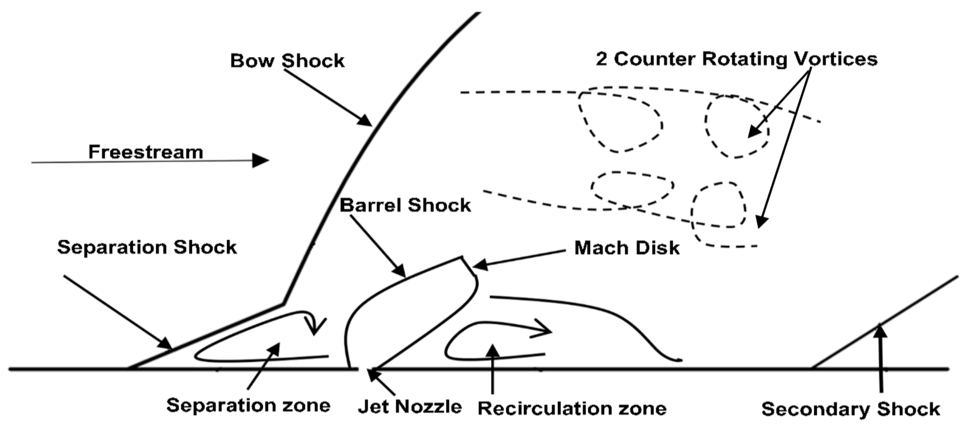
With continuous improvements in maneuverability of targets, traditional aerodynamic rudder control can no longer meet the requirements of precise strikes. Using lateral jet force to control tactical missile attitude and trajectory not only has a rapid response and high efficiency but can also possess effective control at high altitude [1]. Direct force is usually provided by a gas engine that produces lateral jets, and in a high-altitude, low-pressure area, higher requirements are placed on the performance of the gas engine [2,3]. As shown in Figure 1, a complex flow structure exists in the flow field due to interaction between the free stream and the nozzle jet [4]. Under action of incoming flow, the lateral jet is deflected to form a barrel-shaped shock wave and a Mach disk structure, and, at the same time, acts as an obstacle on the surface of the projectile. Therefore, bow shock is formed in the supersonic incoming flow in front of the jet obstruction, while in front of the nozzle, the boundary layer is separated due to the adverse pressure gradient that forms separation shock. At the same time, a low-pressure recirculation zone is formed behind the nozzle. The reflected shock wave acts on the surface of the model and results in secondary shock-wave interference. A pair of antisymmetric vortex structures are generated in the separation zone in front of the nozzle and interact with each other to form a horseshoe vortex near the model wall. The antisymmetric wake vortex interferes with the shock wave in the downstream flow, further enhancing mixing of the supersonic free stream and the jet [5,6]. The complex flow structure requires better material properties for the model shell and internal engine [7,8,9]. For simulation of lateral jet interaction flow, an effective approach is to use an unstructured hybrid grid [10]. However, in an unstructured grid, resolution is usually improved via uniform refinement, and level of refinement is determined empirically. This method increases computational cost. Mesh adaptation can automatically adjust grid distribution and density according to flow characteristics of the flow field in order to improve resolution of the flow with a smaller mesh scale, if possible.
Mesh adaptation technology first emerged in the 1970s, and great progress has been achieved in the fields of error estimation, optimization of grid distribution and object surface grid geometry projection. Grid-distribution optimization can be divided into three types: namely, local grid calculation with precision format upgrade (p-type), grid node movement (r-type) and local grid refinement (h-type) [11]. The p-type method adaptively selects the order of the used numerical scheme according to flow features. However, it is more difficult to program than other methods, so it is rarely used. The r-type method moves grid nodes adaptively according to flow features without changing topology of the grid; however, its ability to change grid distribution is limited, so its application to 3D complex geometries is also limited. Moreover, h-type adaptation refines or coarsens mesh by dividing or merging cells to change grid distribution and improve local resolution of key regions with changing mesh topology [12,13]. From the perspective of engineering applicability, the unstructured hybrid grid is widely used for complex geometries, and it is suitable for h-type adaptation.
Considering the interference flow field of lateral jets, this paper proposes an adaptive criterion combination method to capture and identify the shock wave and vortex structure in the lateral jet interaction flow field. Through adoption of h-type grid adaptive technology, adaptive numerical simulation of the interference flow field under steady and unsteady conditions was carried out. Compared with the uniformly refined mesh results, the simulation results verified that the adaptive criterion combination method developed in this paper can effectively improve flow structure of the lateral jet disturbance flow field.
2. Hybrid Mesh Adaptive Method
2.1. Numerical Simulation Method
Three-dimensional unsteady compressible Reynolds-averaged Navier–Stokes equations were employed as the governing equations for the flow simulation; in the Cartesian coordinate system, they can be written as:
where denotes the vector of conserved quantities; , and are the vectors of convective fluxes; and , and are the vectors of viscous fluxes.
The finite volume approach was used for discretization, the second-order precision format was adopted for spatial discretization [14], the viscous term was discretized by the central difference and the implicit scheme was employed for temporal discretization with the LU-SGS method [15]. The SA one-equation model was adopted for turbulence closure [16]. The wall was adiabatic and no-slip. At the far-field boundary, the Riemann condition was imposed.
The dynamic unsteady calculation adopts the dual time-stepping method to solve the flow control equation under the specified pitching-motion form and parameters. First, the flux tensor, E (including the inviscid term and the viscous term ), was used to simplify Equation (1) and discretize it as Formula (2):
Here, represents net flux passing through the control volume (E), including inflow and outflow grid units, and V is the reciprocal of the Jacobian. Due to overall change in the grid during the pitching process, no local deformation occurs, so the dynamic grid is realized with rigid rotation technology. Formula (2) is written as:
The pseudo-time step τ is introduced here, the superscript n indicates the real-time step and the unsteady implicit calculation format is:
The superscript p represents the pseudo-time step and W represents the original variable. The iterative formula of linearization after discretization is:
In the iterative equation, if , then Formula (4) is established, and the time satisfies the second-order precision [17].
2.2. Adaptation Strategy
The h-type adaptation was adopted to refine and coarsen the unstructured hybrid grid, and cell distribution was optimized via division and merging of cells.
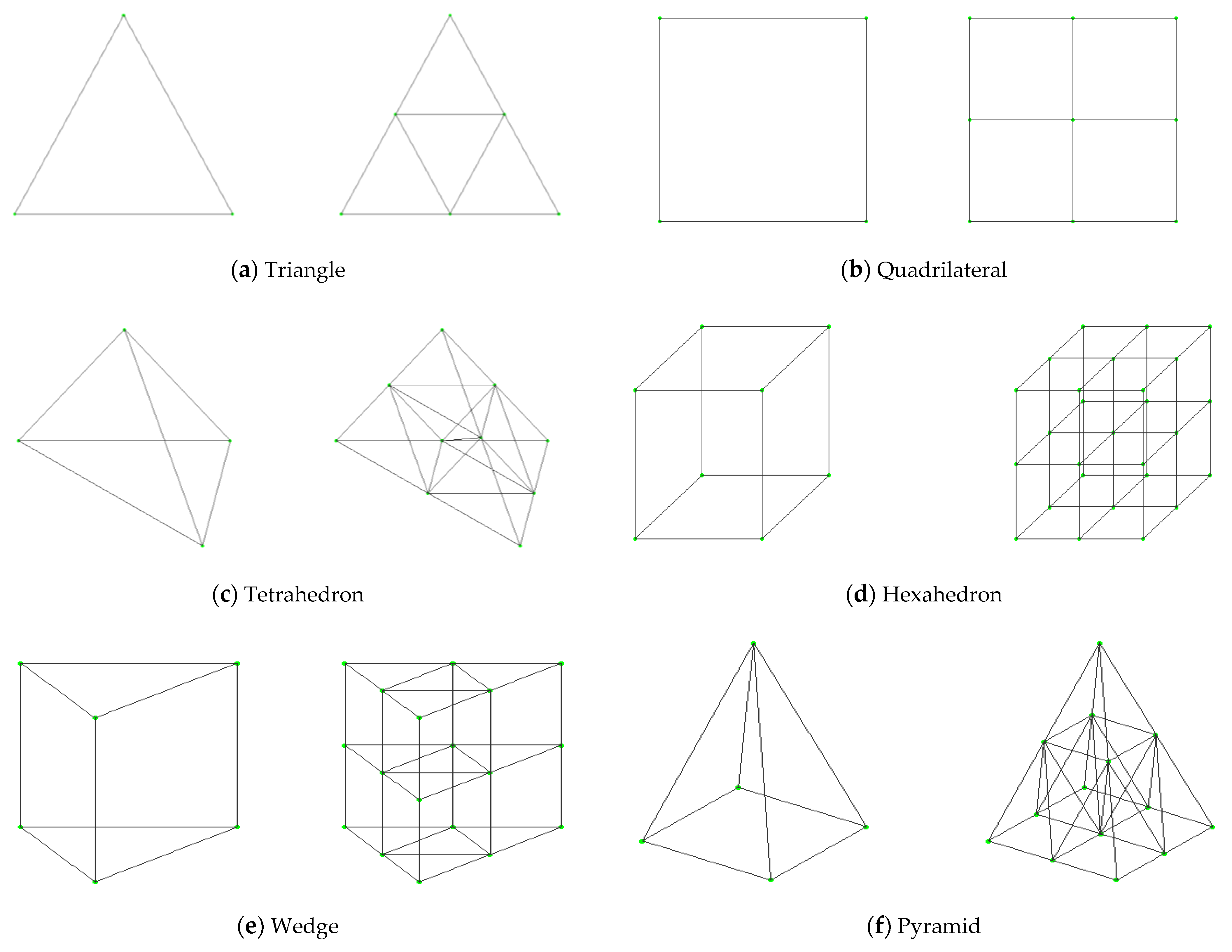
Surface mesh is usually composed of two types of cells: triangular and quadrilateral. Spatial mesh is usually composed of four types of cells: tetrahedral, pyramidal, wedge and hexahedral. With comprehensive consideration of robustness and efficiency of the refinement schemes, isotropic refined cells were selected; each type of cell corresponded to a unique refinement mode. Figure 2 shows subdivision of different cells. After mesh refinement, the spatial mesh was smoothed with Laplacian smoothing to improve geometrical quality. At the same time, combined with the criterion of mesh geometrical quality, the minimum value of the geometrical criterion remained unchanged, and the overall geometrical quality of the mesh was improved as far as possible.
The basic idea of Laplacian smoothness is to move a node to the centroid of a graph surrounded by all nodes that are directly connected to the node through grid edges, so as to improve overall grid quality. The moving distance of the i-th node is:
where is the moving distance of node i, N is the total number of nodes directly connected to node i through grid edges and is the vector that directly connects node i and node k. Multiple instances of smoothing will evenly distribute mesh, and quality of mesh near the object surface will deteriorate. The purpose of this is to ensure grid quality, and thus the number of smoothing times must be limited [18].
Cell coarsening is an inverse process of refinement. In this paper, a “backward” method was used for grid coarsening. Before coarsening, it is necessary to establish the relationship between grid cells at different levels. This is known as the “parent–child” relationship. When all child cells of a parent cell are marked as “coarsening needed”, the parent cell recovers to the state before refinement. If a cell reaches the initial level, the coarsening process is no longer performed [19].
2.3. Adaptive Criteria
To accurately capture change in flow structure in grid adaptation, selection of an adaption criterion is an important task. In this paper, an adaptation criterion based on flow features (such as shock waves and vortices) was used to automatically capture regions where the flow changed severely, making computed results more accurate and reasonable.
2.3.1. Quasi-Gradient-Based Adaptation Criterion
We used gradient of the flow variable as the adaptation criterion because discretization errors may have been large in the region where the flow field changes greatly. The flow variables we used were temperature, pressure, magnitude of velocity and density. The combination of the weighted flow variables can be expressed as:
where is temperature, is pressure, is the modulus of velocity and is density. are the weights of the four variables. The quasi-gradient expression [21] of the flow field variable is:
where I = 1, 2, …, N; N is the total number of units; is cell volume; r is a constant (2 for two dimensions and 3 for three dimensions); and δ is weight of the volume gradient, with a value from 0 to 1.
During the calculation, if a cell evaluates and satisfies , then it needs to be refined, and if a cell evaluates and satisfies, then it needs to be coarsened. Where is the maximum value in the flow field, and are the threshold parameters of adaptive refinement and coarsening.
2.3.2. Adaptation Criterion Based on Curl and Gradient of Velocity
The criterion based on the curl and gradient of velocity [22] was used to identify the free shear vortex and shock structure in the lateral jet flow. It can be expressed as:
where ; N is the total number of cells; and ( is the cell volume), with equal to 2 for two-dimensional problems and 3 for three-dimensional problems. The standard deviation of the two parameters is defined as follows [23]:
During the calculation, for the given threshold function , if the condition of is met in a cell, it needs to be refined. In addition, if a cell satisfies , it needs to be coarsened. Similarly, for the given threshold function , if a cell satisfies , it needs to be refined, and it needs to be coarsened if in it. Here, , , and are the threshold parameters of adaptive refinement and coarsening, respectively.
2.3.3. Adaptation Criterion Based on Vortex Vector
The vortex-vector criterion is a new vortex identification criterion proposed recently by Tian et al. [24]. Compared with the traditional Q criterion, the vortex-vector criterion can capture not only main vortex structures but also more small vortices. In addition, it can exclude shear information that is always identified as a vortex structure by the Q criterion. Therefore, the vortex-vector criterion is more suitable for identification of complex vortex structures. In this work, it is used as the criterion for identifying vortex structures in the lateral jet interaction flow. The vortex vector (R), representing local fluid rotation, is defined as follows:
where , is local fluid rotational angular velocity and is the local fluid-rotational axis. In order to solve for local fluid rotation angular velocity, it is necessary to convert the reference frame xyz to a new reference frame: XYZ. The new reference frame is a local coordinate system with as the Z-axis, and the velocity gradient tensors in the reference frame are xyz and XYZ, respectively:
The velocity-gradient-tensor relationship between the two reference frames can be described as:
where is the transformation matrix from the coordinate system xyz to the coordinate system XYZ [25]. The expression of the vortex vector (R) is as follows:
Standard deviation of the vortex vector (R) is defined as:
During the calculation, for the given threshold function , if a cell satisfies , then it needs to be refined, and it needs to be coarsened if in it. and are the threshold parameters of adaptive refinement and coarsening.
2.4. Combined Adaptation Criteria
Lateral jet interference flow contains complex structures, such as shock waves and vortices, that are difficult to accurately detect and identify using a single adaptation criterion. Therefore, the method of combing multiple adaptation criteria was employed to analyze the lateral jet interference flow field.
The following judgments are utilized:
- (1)
- If a mesh cell satisfies and , then it needs to be refined. This identifies shock waves in the flow field.
- (2)
- If a mesh cell satisfies or , then it needs to be refined. This identifies vortex structures in the flow field.
- (3)
- If a mesh cell satisfies or , then it needs to be coarsened. This identifies absence of shock waves in the flow field.
- (4)
- If a mesh cell satisfies and , then it needs to be coarsened. This identifies absence of a vortex in the flow field.
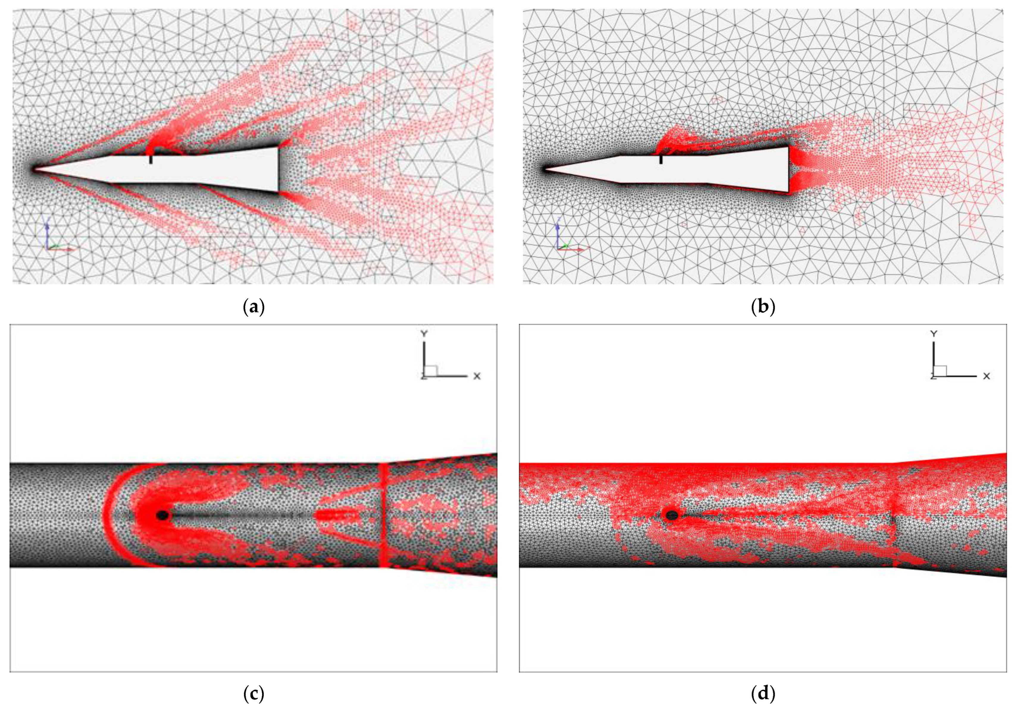
Using the model and calculation conditions described in Section 3.1, we obtained results of different combinations of methods. Figure 3a,c show mesh results under Criterion (1) (refinement) and Criterion (3) (coarsening), and it can be seen that this combination method can more accurately identify shock-wave structure in the flow field as well as surface structure of the model. Figure 3b,d show the mesh results under Criterion (2) (refinement) and Criterion (4) (coarsening). This combination method is better for capturing vortex structure, but is not as beneficial for identification of surface structure of the model.
For the structural regions identified by the methods above, another combination is required. A combined adaptation criterion for simulating a lateral jet interaction flow field was constructed in the following way: In the boundary layer, cells that satisfy Criterion (1) are marked to be refined, and those that satisfy Criterion (3) are marked to be coarsened. In the regions outside of the boundary layer, cells that satisfy Criterion (1) or (2) are marked as refined cells, and the cells that satisfy both Criterion (3) and Criterion (4) are marked to be coarsened. , , and (i = 1, 2, 3) are criterion control parameters; parameters are selected empirically for different flow conditions.
2.5. Frequency Selection for Dynamic Grid Adaptation
The dynamic grid adaptation was used to automatically capture features of unsteady flows involving moving bodies, and at the same time, the grid in the region near the transverse jet would also be refined or coarsened dynamically. The adaptation criteria have been described above, and frequency of dynamic adaptation () needed to be predetermined. is defined as the ratio of the time interval of each adaptation () to the time step of the flow calculation (). The interval of grid adaptation () also needed to be predetermined and is related to the minimum cell size of the base grid (hmin) and characteristic length of the concerned flow structure (Lv); its value is in the following range () [23]:
where is reference velocity (generally taken as free-flow velocity) and is characteristic length of the shock wave in the lateral jet interference flow (taken as the distance between the beginning and the end point of bow shock on a symmetrical plane in this paper). Therefore, the range of adaptation frequency () is:
3. Adaptive Simulation of Lateral Jet Interaction Flow Field
3.1. Generic Missile Model and Flow Conditions
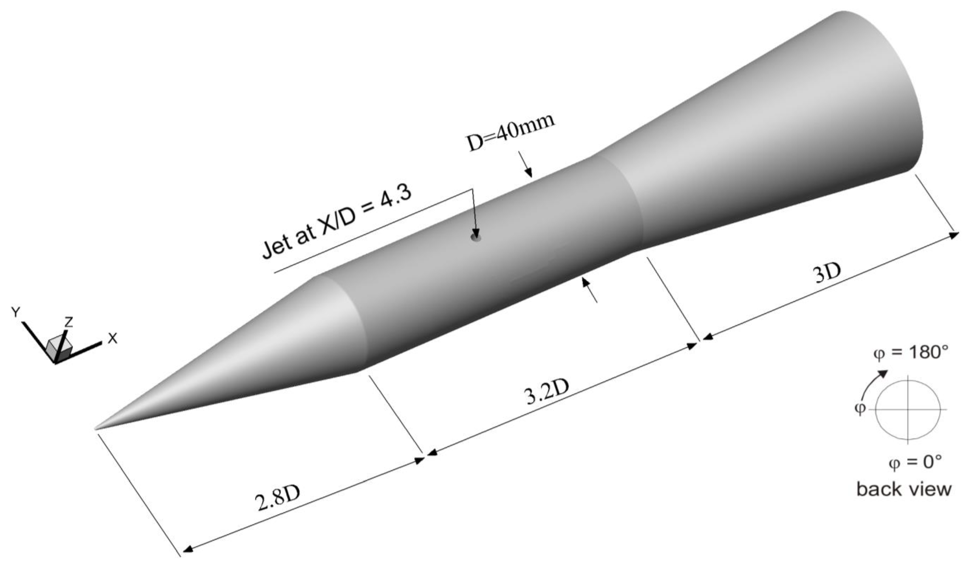
In this work, the standard model of the lateral jet [26] was used to test the ability of the present grid adaptation method. As shown in Figure 4, the standard model consists of a cone-shaped nose, a cylindrical body (diameter D = 40 mm) and an adjacent flared afterbody, which in turn is connected to a cylindrical aft extension. A circular sonic-side jet nozzle of 4 mm (0.1 D) in diameter is located on the cylindrical midsection at an azimuth of ϕ = 180° and a position of X = 4.3 D downstream from the model tip. The jet axis is perpendicular to the longitudinal axis of the model. Since the centroid position of the model was not specified in the referenced article [26], in this work, the model was assumed to be homogenous and the centroid position xcg = 6.05 D. The free-stream condition was as follows: Mach number = 2.8, static temperature = 108.96 K, static pressure = 20,793.2 Pa, Reynolds number = and angle of attack = 0°. The pressure ratio of the jet was (the total pressure of the jet divided by the static pressure of the free stream), and the static temperature of the jet was the same as that of the free stream.
Adaptive combined criteria were as described in Section 2.4, and in Formula (7), pressure was selected as the gradient variable (the pressure on the weight of the flow-field variable was 1, and the weights of the other variables were 0 each). In order to accurately identify essential structures in lateral jet interference flow, achieve a reasonable distribution of adaptive mesh and reduce computational cost, the parameters of the adaptation criterion were specified as:
3.2. Transverse Jet Efficiency
In order to accurately describe the actual control effect of the lateral jet in different situations, we obtained the overall effect of the jet on the model, and the concept of the amplification factor was introduced [5]. The force-amplification factor () and the moment-amplification factor () were defined:
where and are aerodynamic force and moment due to interference between the jet and the supersonic flow, and and are aerodynamic force and moment directly generated by the jet. The related expressions are [27]:
In Formula (25), and are aerodynamic force and moment without jet interference, respectively; and are aerodynamic force and moment with jet interference, respectively; is the gas-specific heat ratio, is the Mach number at the jet outlet, is pressure at the jet outlet, is area at the jet outlet, is pressure of the incoming flow and is the distance from the nozzle to the centroid.
3.3. Simulation of a Steady Flow
The total cell number of the base mesh was about 1.71 million. The initial flow field was iterated via 10,000 time steps, and the number of iterations was also 10,000 after each mesh adaptation. The base mesh was adapted twice. In order to verify reliability and effectiveness of the present mesh adaptation method, the base mesh was refined uniformly, and the total cell number of the refined mesh was about 30 million.
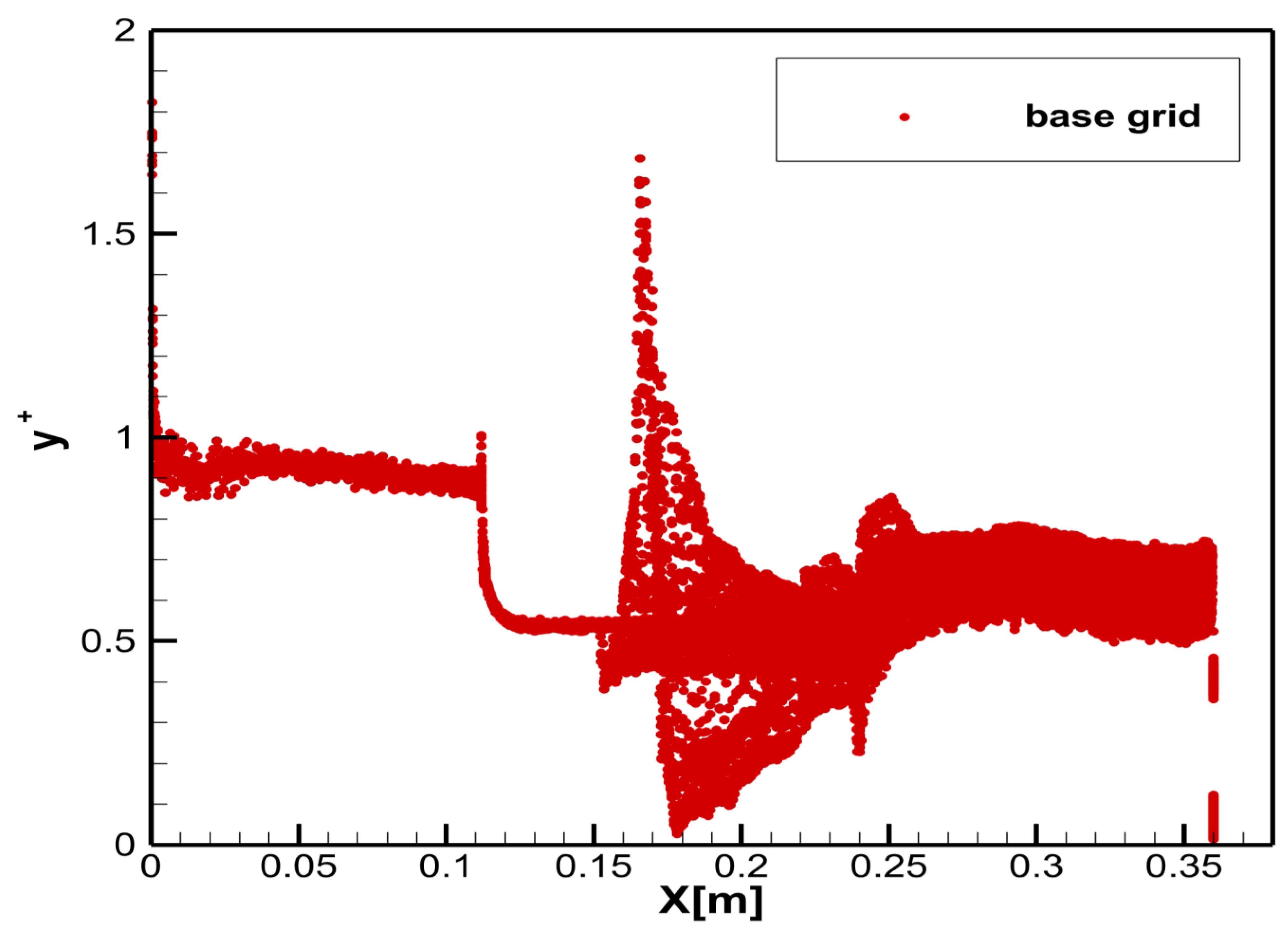
The first boundary-layer height was set as m to ensure that the y+ value was around 1. From the conducted analyses, y+ values were exported from the generated meshes and are presented in Figure 5.
Upon examination of Figure 5, it can be seen that the y+ value is below 1, except in the jet vicinity. Due to separation and recirculation in the jet vicinity, the y+ value increased in that region, which was an expected situation and shows that the first grid height in the boundary layer was adequate for a jet in a cross-flow case.
Total cell numbers for the base mesh and adapted meshes are presented in Table 1. Growth rate is the ratio of the difference between the cell number from the adaptive mesh and that of the base mesh, and the cell number from the base mesh. Numerical simulation used 110 cores for parallel computing, and the simulation times for the original grid, adaptive primary grid, adaptive secondary grid and globally refined grid were about 0.6 h, 1.5 h, 6.3 h and 15 h, respectively.
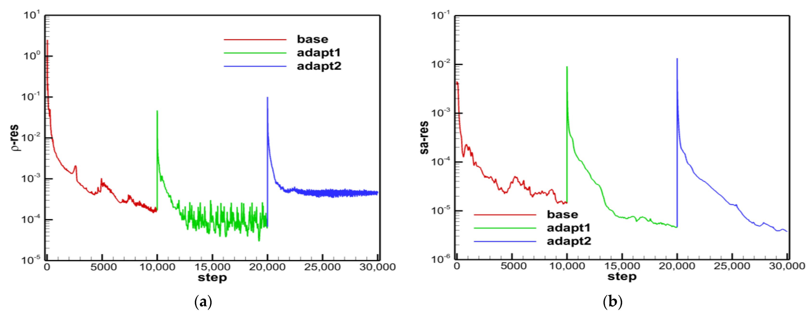
Figure 6a shows the convergence history of residual density during the mesh adaptation. It can be seen that the convergence rate of residual density was significantly improved and more stable after each adaptation, but the residual value of the twice-adapted result was higher. Figure 6b shows the SA turbulence—residual convergence curve during the adaptive simulation process. After adaptive simulation, convergence of residual turbulence was significantly improved, with a greater magnitude of decline and faster speed.
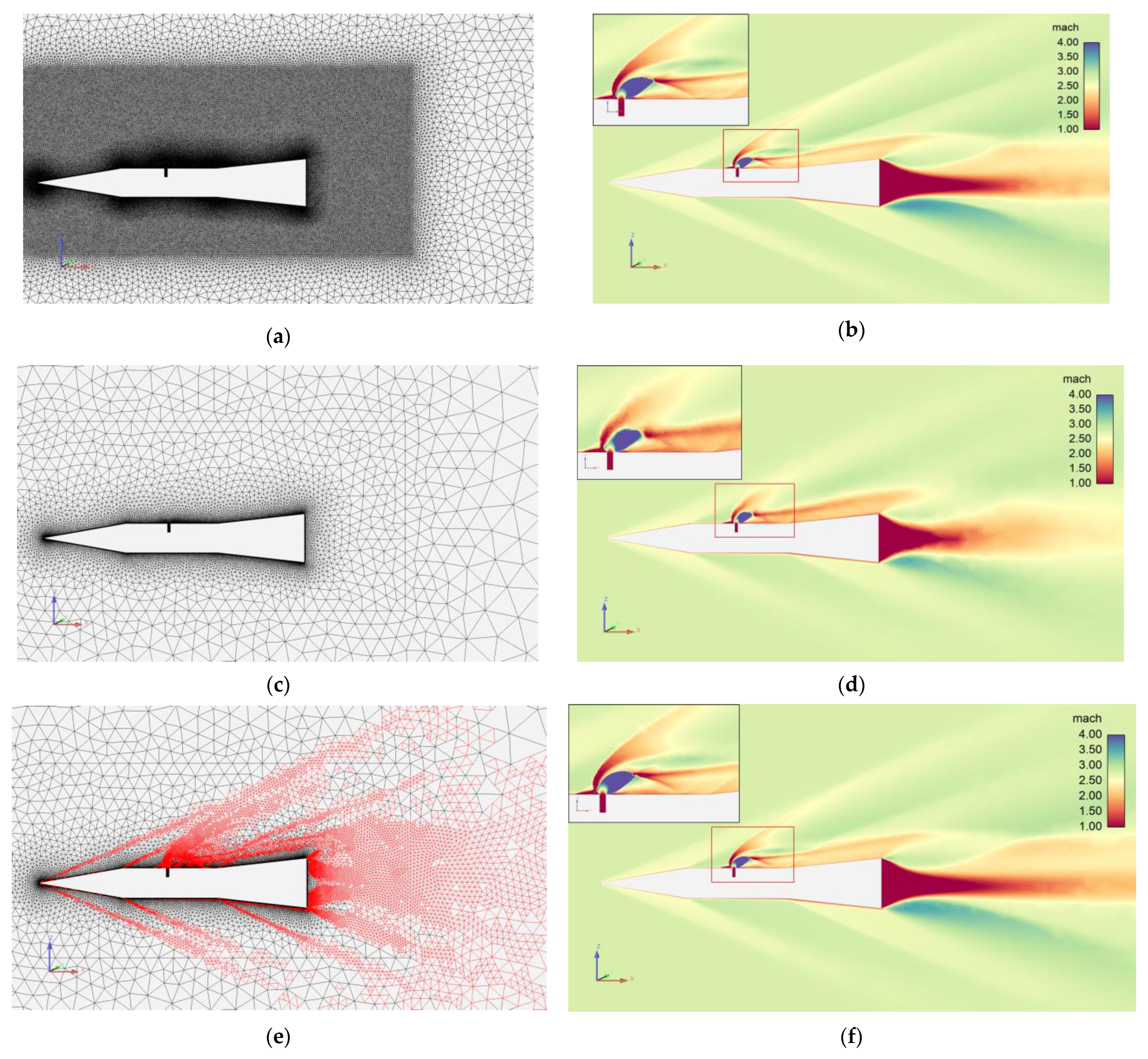
Figure 7 shows the uniformly refined base and adaptive meshes on the symmetry plane of the flow field and the corresponding computed contours of the Mach number. It was found that after adaptive refinement, details of the flow, such as shock-wave interference and vortex structure, were captured much more effectively, and resolution of the flow field was greatly improved. The flow fields computed on the uniformly refined mesh and on the adaptively refined mesh were very close to each other.
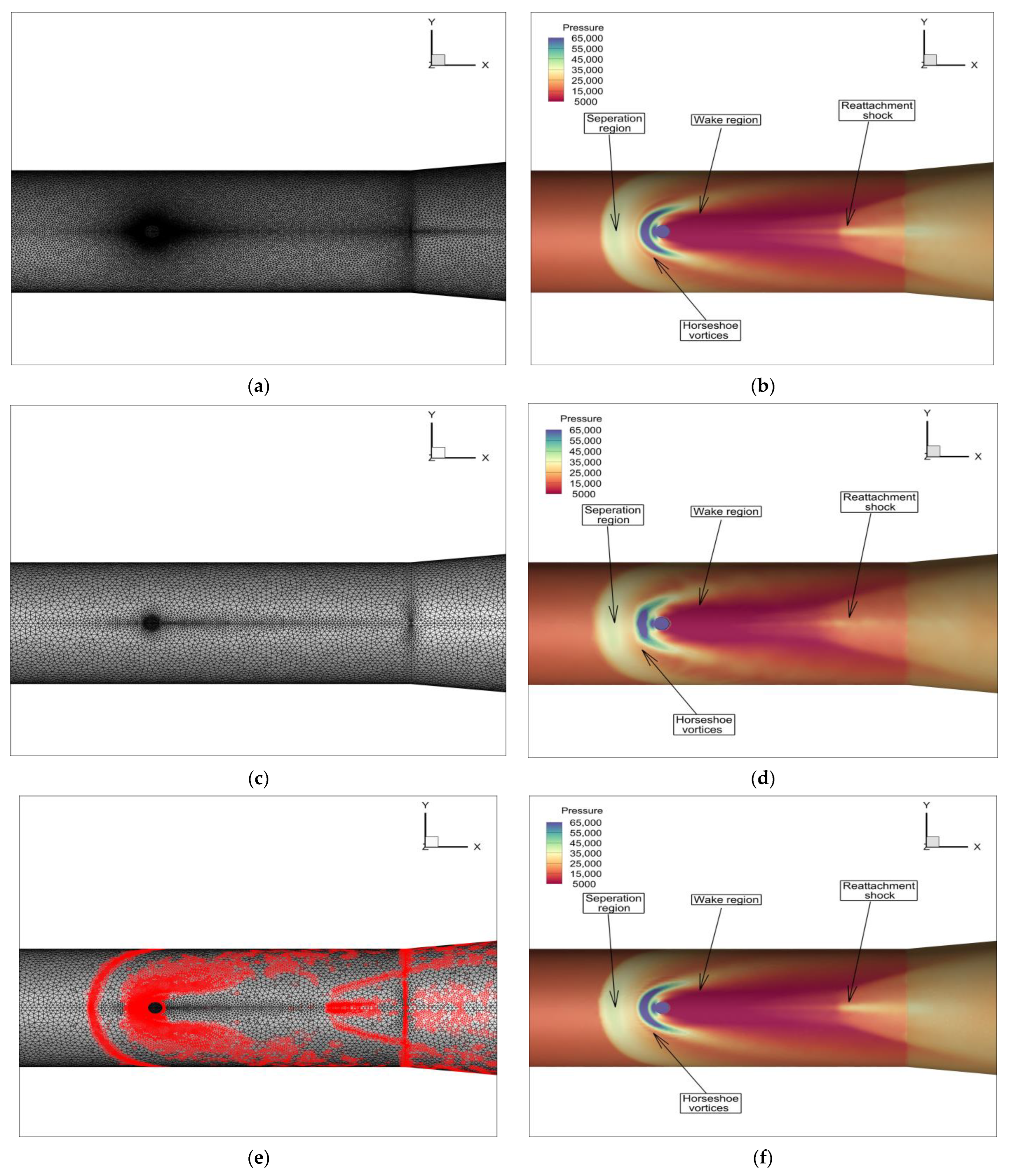
Figure 8 shows the surface mesh and the corresponding contours of pressure on the surface for the uniformly refined base, as well as adaptive meshes before and after global encryption and self-adaptation. It can be seen that the adaptation criterion accurately captures the border of the high-pressure separation zone, horseshoe vortices, the wake region and reattachment shock on the model surface, and pressure distribution on the surface was largely improved.
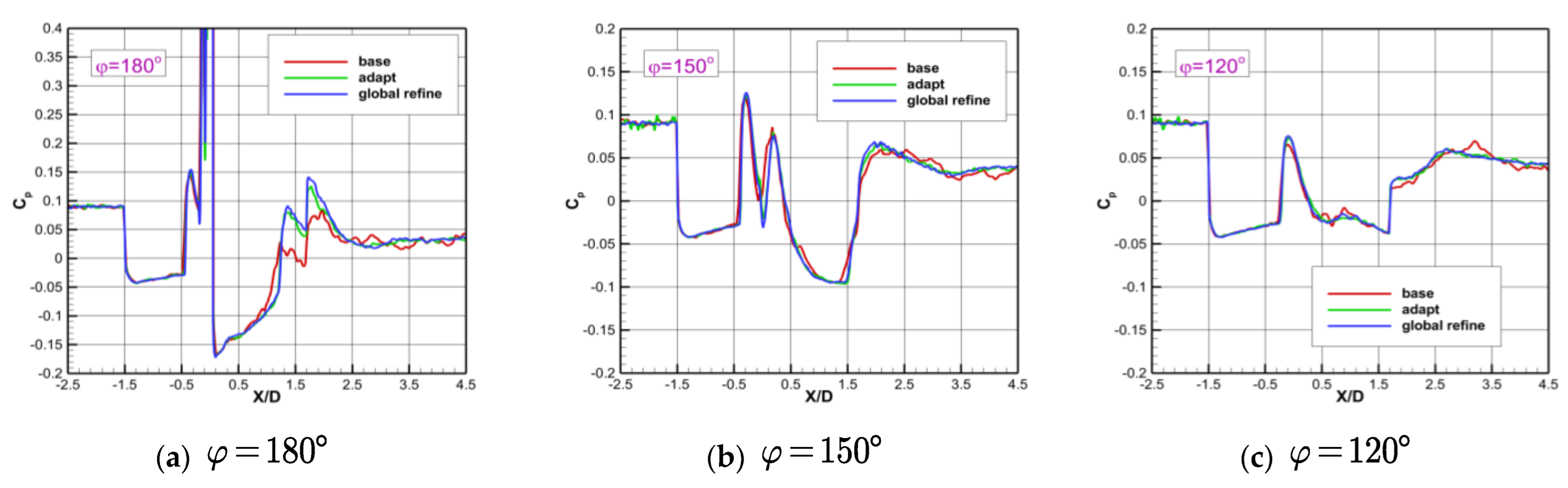
Figure 9 shows distribution of pressure coefficients on the model surface for different azimuth angles. These results show that pressure distribution after adaptation is more stable and reasonable, and fits better with the globally refined mesh. The results computed for the adaptive mesh are much closer to those computed for the uniformly refined mesh. In quantitative comparison of pressure coefficients between different meshes, it could be seen that the relative error was largest on the 180° axis. The errors between the base mesh, adaptive mesh and uniformly refined mesh were 92.1% and 12.3%, respectively.
3.4. Simulation of an Unsteady Flow
In order to verify reliability of the technique of dynamic mesh adaptation, a simulation of an unsteady flow field involving pitching motion of the lateral jet was carried out. Boundary conditions were consistent with the steady calculation. The time step (Δt) was 1/500 of the pitching cycle, the number of inner iterations within each physical time step was 40 and frequency of the dynamic mesh adaptation was determined according to Formula (22). In the base grid, and . The mesh adaptation dynamic frequency was taken as 20 and the maximum level of adaptation as 2. Three oscillation cycles were simulated. The forced pitch motion is described by the variation in the pitch angle with time [28]:
where is the mean angle of pitching, is pitching amplitude, is circular frequency and is frequency. The reduced frequency is defined as:
where denotes diameter of the bullet body. The reduced frequency was 0.107, the mean angle of pitch motion was 0° and the pitching amplitude was 5°. In the process of the unsteady simulation calculation, the maximum number of adaptive grids was 24.42 million, and the simulation time of one cycle was about 50 h.
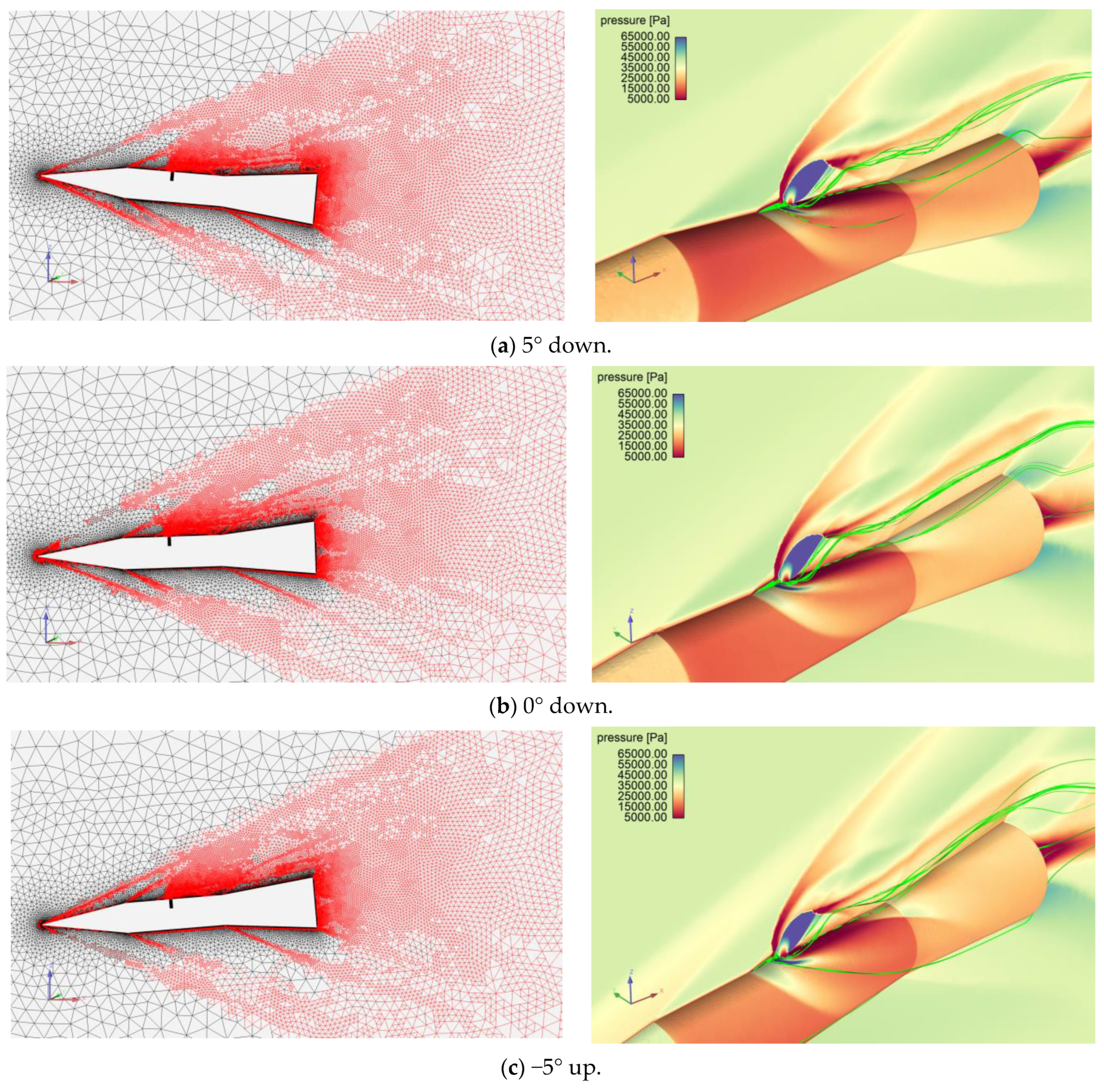
Figure 10 shows adaptive meshes on the symmetry plane and their corresponding flow structures. From the plotted streamlines and the contours of pressure, it can be seen that detailed features in unsteady flows were captured with a high resolution. Effectiveness of the dynamic mesh adaptation for simulation of unsteady flows was verified. It can also be seen that, compared with the steady results, the range of mesh refinement was larger in the unsteady flow simulation, but was still mainly concentrated in the region containing the shock waves and vortices, and the total number of mesh cells also increased to about 20 million at 0°.
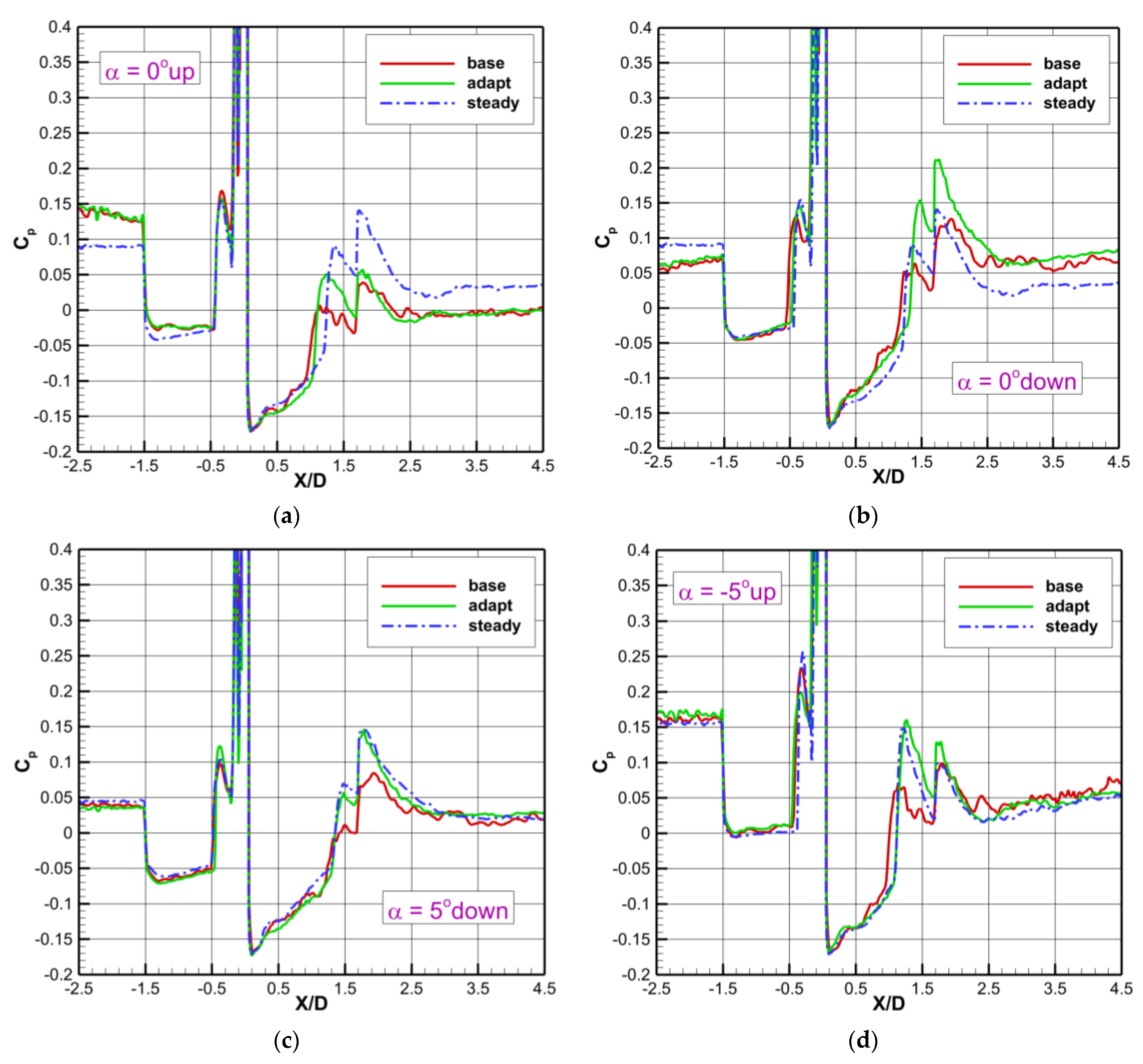
Figure 11 shows distribution of pressure coefficients on the meridian for different pitching angles within one cycle of lateral jet projectile vibration. It can be seen from the figure that the computed results on the base mesh are significantly different from those on the adaptive meshes. In comparison of distribution of pressure coefficients in the steady state, it was found that the unsteady effect was most obvious for the 0° attack angle. The distribution of pressure coefficients at the angle of was significantly different, and those differences were mainly concentrated in the areas in front of and behind the nozzle jet. At the angle of attack of 0°, the difference between the results computed with adaptive meshes for moving up and down was significant, but the difference obtained with the base mesh was not obvious. This indicates that it was difficult for the base mesh to effectively identify any unsteady effects, while the dynamic adaptive mesh could capture unsteady phenomena more easily.
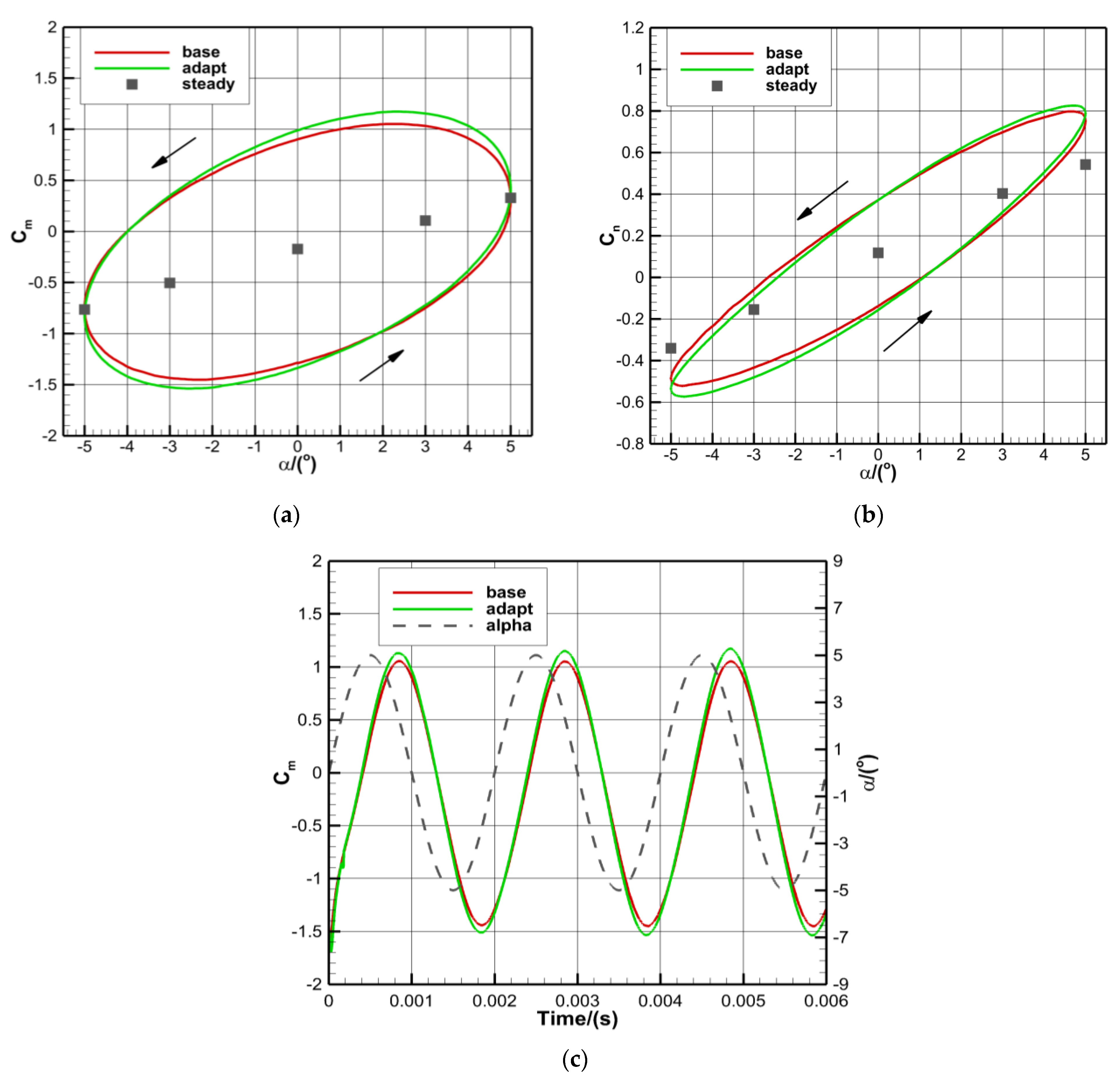
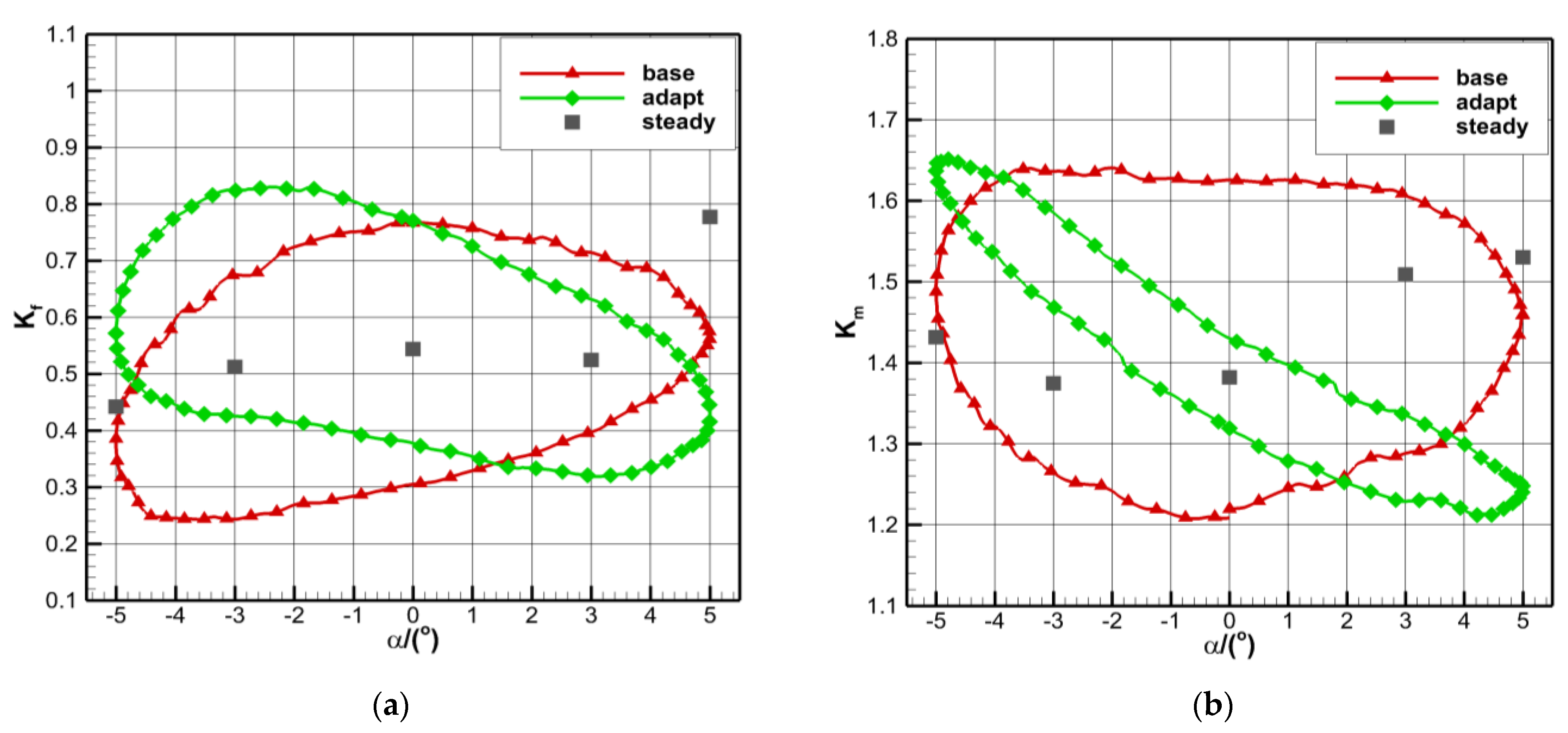
Figure 12 shows variations in the pitching-moment coefficient and in the normal-force coefficient with the angle of pitching. The solid points in the figure represent values at a fixed angle of attack, and obvious dynamic hysteresis can be seen. In comparison of the results of the base and adaptive meshes, it can be seen that the difference between aerodynamic coefficients was not large. From Figure 12c, a significant phase lag in computed results can be seen. Additionally, aerodynamic coefficients were significantly different near the 0 degree angle of attack. Combination with the results of surface distribution of pressure coefficients shows that the proposed adaptation criterion plays an important role in improving aerodynamic calculation of complex lateral jet interaction flows.
Figure 13 shows variation in thrust and moment-amplification factors with the angle of attack. Compared with the steady calculation results, amplification factors changed nonlinearly. Through force and moment-amplification factors, the effect of dynamic mesh adaptation on the interference structure between the jet and incoming flow can be compared and analyzed. Obvious differences were found between the results of the adaptive meshes and those of the base mesh. The moment-amplification factor obtained with the base mesh changed slightly at around 0 degrees, while the adaptive-mesh result changed significantly. Due to the strong unsteady effect at 0 degrees, it can be said that the lateral jet interference flow field was not accurately simulated with the base mesh, and jet interference structures were captured poorly. It was also shown that dynamic mesh adaptation significantly improved prediction of unsteady lateral jet interference structure.
4. Summary
In this paper, a mesh adaptation method was established for simulation of a lateral jet interaction flow field, and numerical experiments for steady and unsteady lateral jet interaction flows on adapted meshes were carried out. The following conclusions were obtained:
- (1)
- A combined adaptation criterion for unstructured hybrid mesh is proposed for simulating lateral jet interaction flows. This can effectively capture complex structures in the lateral jet interaction flow field, such as shock waves and vortices.
- (2)
- The proposed adaptation criterion can significantly improve convergence of flow computation and resolution of flow structures. It also plays an important role in numerical simulation of lateral jet interaction flows and improves prediction accuracy of the aerodynamic characteristics of a missile.
- (3)
- Compared to the uniformly refined mesh, the adaptive mesh had a similar resolution to the flow field, while the total number of mesh cells was much smaller. Additionally, in this way, computational efficiency can be improved greatly.
- (4)
- The present adaptation criteria can identify characteristic structures in the unsteady flow field and effectively improve resolution of flow and accuracy of aerodynamic calculation.
- (5)
- In parallel computing, adaptive refined mesh may be concentrated in one processor in such a way that seriously imbalanced distributed mesh cannot reduce computational cost effectively. Implementation of dynamic load balancing in the solver for parallel computing will be the focus of future research.
Author Contributions
Conceptualization, S.T. and Z.P.; methodology, Z.P.; formal analysis, Z.P.; investigation, S.T. and Z.P.; validation, Z.P.; resources S.T.; writing—original draft preparation, Z.P.; writing—review and editing, S.T. and Z.P.; visualization, Z.P.; supervision, S.T.; project administration, S.T.; funding acquisition, S.T. All authors have read and agreed to the published version of the manuscript.
Funding
This research was funded by the Industry University Research Cooperation Fund of the Eighth Research Institute of China Aerospace Science and Technology Corporation grant number SAST2020-07.
Data Availability Statement
Not applicable.
Acknowledgments
This work was financially supported by the Industry University Research Cooperation Fund of the Eighth Research Institute of China Aerospace Science and Technology Corporation (Grant No. SAST2020-07). This research was also supported in part by the Priority Academic Program Development of Jiangsu Higher Education Institutions.
Conflicts of Interest
The authors declare no conflict of interest.
References
- Zhang, Y.J.; LI, S.H.; Zhu, H.B. Research on Modeling and Simulation of Optimal Search of Multifunction Phased Array Radar. J. Syst. Simul. 2008, 20, 4248–4251. [Google Scholar]
- Saif, U.K.; Saqib, H.; Ali, H.M.; Shehar, B.; Muhammad, A.N.; Naseem, A. Experimental investigation of aluminum fins on relative thermal performance of sintered copper wicked and grooved heat pipes. Prog. Nucl. Energy 2022, 152, 104374. [Google Scholar] [CrossRef]
- Siddiqi, H.-U.; Qamar, A.; Shaukat, R.; Anwar, Z.; Amjad, M.; Farooq, M.; Abbas, M.M.; Imran, S.; Ali, H.; Khan, T.; et al. Heat transfer and pressure drop characteristics of ZnO/DIW based nanofluids in small diameter compact channels: An experimental study. Case Stud. Therm. Eng. 2022, 39, 102441. [Google Scholar] [CrossRef]
- Lee, J.W.; Min, B.Y.; Byun, Y.H.; Lee, C. Numerical Analysis and Design Optimization of Lateral Jet Controlled Missile. In Proceedings of the 21st International Congress of Theoretical and Applied Mechanics, Warsaw, Poland, 5–21 August 2004. [Google Scholar]
- Gnemmi, P.; Schäfer, H.J. Experimental and Numerical Investigations of a Transverse Jet Interaction on a Missile Body. In Proceedings of the 43rd AIAA Aerospace Sciences Meeting and Exhibit, Reno, NV, USA, 10–13 January 2005. [Google Scholar]
- Christie, R. Lateral Jet Interaction with a Supersonic Crossflow. Master’s Thesis, University of Cranfield, Cranfield, UK, October 2010. [Google Scholar]
- Alqahtani, S.; Ali, H.M.; Farukh, F.; Kandan, K. Experimental and computational analysis of polymeric lattice structure for efficient building materials. Appl. Therm. Eng. 2023, 218, 119366. [Google Scholar] [CrossRef]
- Zawawi, N.N.M.; Azmi, W.H.; Ghazali, M.F.; Ali, H.M. Performance of Air-Conditioning System with Different Nanoparticle Composition Ratio of Hybrid Nanolubricant. Micromachines 2022, 13, 1871. [Google Scholar] [CrossRef] [PubMed]
- Lawag, R.A.; Ali, H.M. Phase change materials for thermal management and energy storage: A review. J. Energy Storage 2022, 55, 105602. [Google Scholar] [CrossRef]
- Baker, T.J. Mesh generation: Art or science? Prog. Aerosp. Sci. 2005, 41, 29–63. [Google Scholar] [CrossRef]
- Baker, T.J. Mesh adaption strategies for problems in fluid dynamics. Finite Elem. Anal. Des. 1997, 25, 243–273. [Google Scholar] [CrossRef]
- Mavriplis, D.J. Unstructured Mesh Generation and Adaptivity: NASA-CR-195069; NASA: Washington, DC, USA, 1995.
- Lohner, R. Adaptive h-refinement on 3D unstructured grids for transient problems. Int. J. Numer. Methods Fluids 1992, 14, 1407–1419. [Google Scholar] [CrossRef]
- Roe, P.L. Approximate Riemann solvers, parameter vectors and different schemes. J. Comput. Phys. 1981, 43, 357–372. [Google Scholar] [CrossRef]
- Yoon, S.; Jameson, A. Lower-upper Symmetric Gauss Sediel method for the Euler and Navier-Stokers equations. AIAA J. 1988, 26, 1025–1026. [Google Scholar] [CrossRef]
- Spalart, P.R.; Allmaras, S.R. A one-equation turbulence model for aerodynamic flows. In Proceedings of the AIAA the Aerospace Sciences Meeting and Exhibit, Reno, NV, USA, 6–9 January 1992. [Google Scholar]
- Lai, J.; Zhao, Z.; Wang, X.; Li, H.; Li, Y. Uniform pitching motion and angular rate effects on transverse jet interaction. Acta Aeronaut. Astronaut. Sin. 2019, 40, 122866. (In Chinese) [Google Scholar] [CrossRef]
- Tang, J.; Zheng, M.; Deng, Y.Q.; Li, B. Grid adaption for flow simulation of complicated configuration. Chin. J. Comput. Mech. 2015, 32, 752–757. [Google Scholar]
- Zhang, P.H.; Tang, Y.; Tang, J.; Luo, L.; Jia, H.Y.; Zhang, Y.B. High Mach number cavity flow simulation based on adaptive unstructured hybrid mesh. J. Beijing Univ. Aeronaut. Astronaut. 2022, 1–12. [Google Scholar] [CrossRef]
- Fluent2020r2/Fluent Theory Guide/Hanging Node Adaption. Available online: https://ansyshelp.ansys.com/account/secured?returnurl=/Views/Secured/corp/v202/en/flu_th/flu_th_sec_adapt_hanging.html?q=Figure%2029.3 (accessed on 15 September 2022).
- Daunenhofer, J.F.; Baron, J.R. Grid Adaption for the 2D Euler Equations. In Technical Report AIAA-85-0484; American Institute of Aeronautics and Astronautics: Reston, VA, USA, 1985. [Google Scholar]
- De Zeeuw, D.L. A Quadtree Based Adaptively Refined Cartesian-Grid Algorithm for Solution of the Euler Equations. Ph.D. Thesis, University of Michigan, Ann Arbor, MI, USA, 1993. [Google Scholar]
- Hu, O. Development of Cartesian Grid Method for Complex Compressible Flows and its Applications. Ph.D. Thesis, Nanjing University of Aeronautics and Astronautics, Nanjing, China, 2013. [Google Scholar]
- Tian, S.; Gao, Y.; Dong, X.; Liu, C. Definitions of vortex vector and vortex. J. Fluid Mech. 2018, 849, 312–339. [Google Scholar] [CrossRef] [Green Version]
- Tian, S.; Fu, H.; Xia, J.; Yang, Y. A vortex identification method based on local fluid rotation. Phys. Fluids 2020, 32, 015104. [Google Scholar] [CrossRef]
- Gnemmi, P.; Adeli, R.; Longo, J. Computational Comparisons of the Interaction of a Lateral Jet on a Supersonic Generic Missile. In Proceedings of the AIAA Atmospheric Flight Mechanics Conference, Honolulu, HI, USA, 18–21 August 2008. [Google Scholar] [CrossRef]
- Geng, Y.F. Numerical Simulation of the New Methods of Drag Reduction and Thermal Protection in the Hypersonic Vehicle Design. Master’s Thesis, Beihang University, Beijing, China, 2011. [Google Scholar]
- Zhao, H.Y.; Liu, W.; Ren, B. Numerical simulation of lateral jets with forced pitching oscillation. Chin. Q. Mech. 2007, 28, 363–368. [Google Scholar]
Figure 1.
Complex flow structure around jet nozzle.

Figure 2.
Subdivision of different cells [20].
Figure 2.
Subdivision of different cells [20].

Figure 3.
Meshes on the symmetry plane and model: (a,b) symmetry mesh and (c,d) model mesh.

Figure 4.
DLR wind-tunnel test model.

Figure 5.
y+ values of the base mesh.

Figure 6.
Residual convergence: (a) density and (b) turbulence.

Figure 7.
Meshes and contours of the Mach number on the symmetry plane: (a) uniformly refined mesh, (c) base mesh and (e) adaptive mesh; (b,d,f) contours of the Mach number on corresponding meshes in (a,c,e).
Figure 7.
Meshes and contours of the Mach number on the symmetry plane: (a) uniformly refined mesh, (c) base mesh and (e) adaptive mesh; (b,d,f) contours of the Mach number on corresponding meshes in (a,c,e).

Figure 8.
Mesh and pressure contour on model: (a) uniformly refined mesh, (c) base mesh and (e) adaptive mesh; (b,d,f) contours of pressure on corresponding meshes in (a,c,e).
Figure 8.
Mesh and pressure contour on model: (a) uniformly refined mesh, (c) base mesh and (e) adaptive mesh; (b,d,f) contours of pressure on corresponding meshes in (a,c,e).

Figure 9.
Distribution of pressure coefficients obtained with different meshes.

Figure 10.
Adaptive meshes, contours of pressure and streamlines at different pitching angles.

Figure 11.
Distribution of pressure coefficients on model surface at different angles of attack.

Figure 12.
Curves for aerodynamic coefficient: (a) variation in pitching-moment coefficient with angle of attack, (b) variation in normal-force coefficient with angle of attack, and (c) variation in pitching-moment coefficient with time.
Figure 12.
Curves for aerodynamic coefficient: (a) variation in pitching-moment coefficient with angle of attack, (b) variation in normal-force coefficient with angle of attack, and (c) variation in pitching-moment coefficient with time.

Figure 13.
Amplification factors of transverse jet interaction: (a) force-amplification factor against pitching angle and (b) moment-amplification factor against pitching angle.
Figure 13.
Amplification factors of transverse jet interaction: (a) force-amplification factor against pitching angle and (b) moment-amplification factor against pitching angle.


Table 1.
Total cell numbers of different meshes.
| Mesh Adaptation | Total Number of Mesh Cells | Growth Rate |
|---|---|---|
| Base mesh | 1.71 million | / |
| Once-adapted | 4.32 million | 155.5% |
| Twice-adapted | 14.22 million | 731.6% |
Publisher’s Note: MDPI stays neutral with regard to jurisdictional claims in published maps and institutional affiliations. |
© 2022 by the authors. Licensee MDPI, Basel, Switzerland. This article is an open access article distributed under the terms and conditions of the Creative Commons Attribution (CC BY) license (https://creativecommons.org/licenses/by/4.0/).
Share and Cite
MDPI and ACS Style
Tian, S.; Peng, Z. Mesh Adaptation for Simulating Lateral Jet Interaction Flow. Aerospace 2022, 9, 781. https://doi.org/10.3390/aerospace9120781
AMA Style
Tian S, Peng Z. Mesh Adaptation for Simulating Lateral Jet Interaction Flow. Aerospace. 2022; 9(12):781. https://doi.org/10.3390/aerospace9120781
Chicago/Turabian StyleTian, Shuling, and Zongzi Peng. 2022. "Mesh Adaptation for Simulating Lateral Jet Interaction Flow" Aerospace 9, no. 12: 781. https://doi.org/10.3390/aerospace9120781
Note that from the first issue of 2016, this journal uses article numbers instead of page numbers. See further details here.