
The Impact of Distributed Propulsion on the Aerodynamic Characteristics of a Blended-Wing-Body Aircraft


Abstract
:1. Introduction
2. Analysis Methods
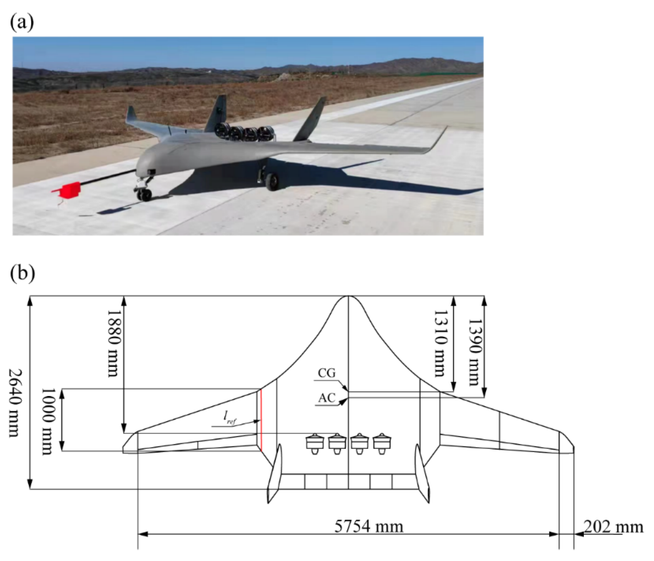
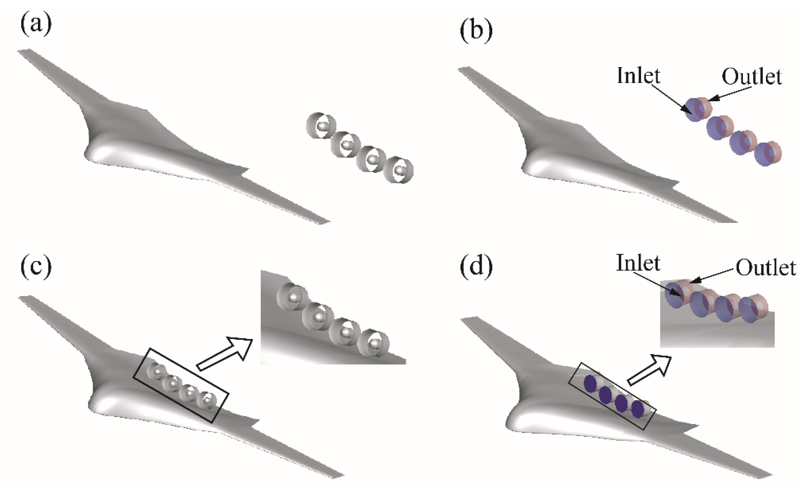
2.1. DPD Model
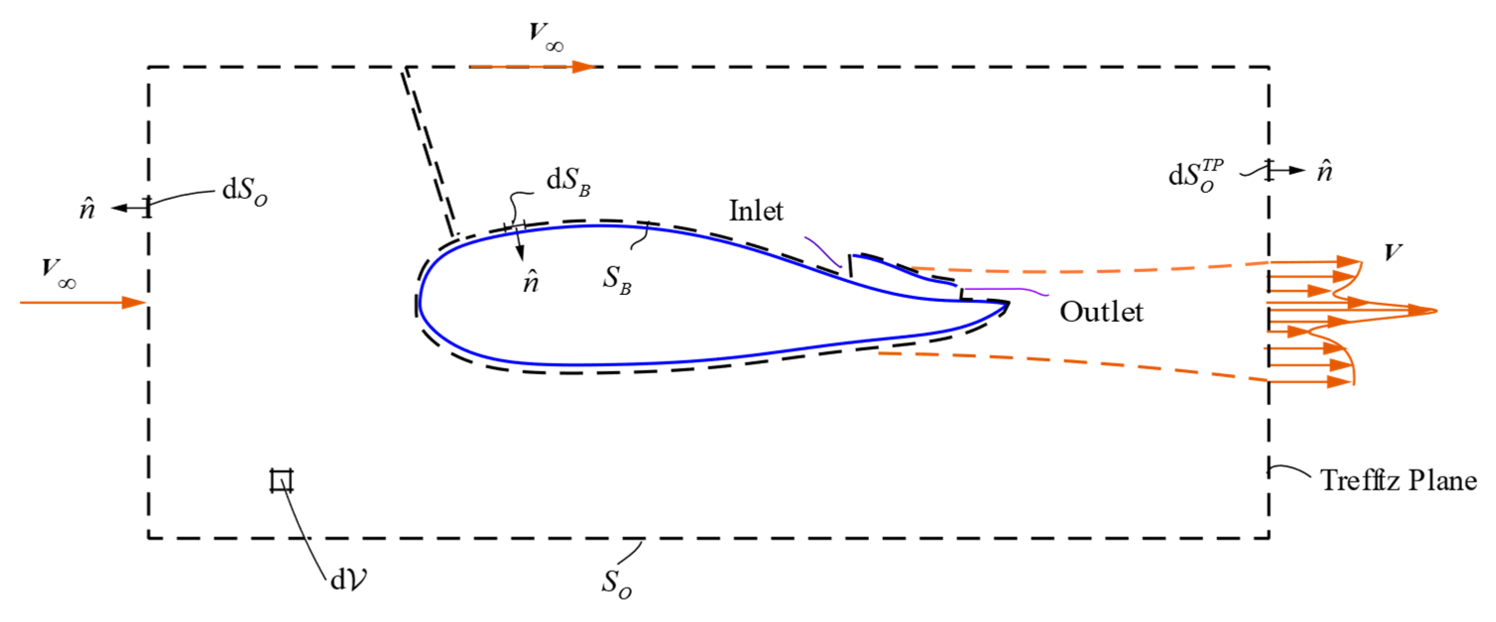
2.2. Aero-Propulsive Integrated Power Balance Analysis
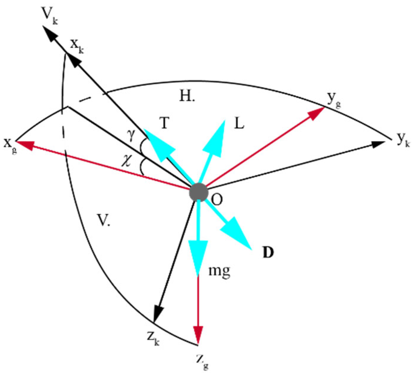
2.2.1. Power Balance in Low-Speed Flow Fields
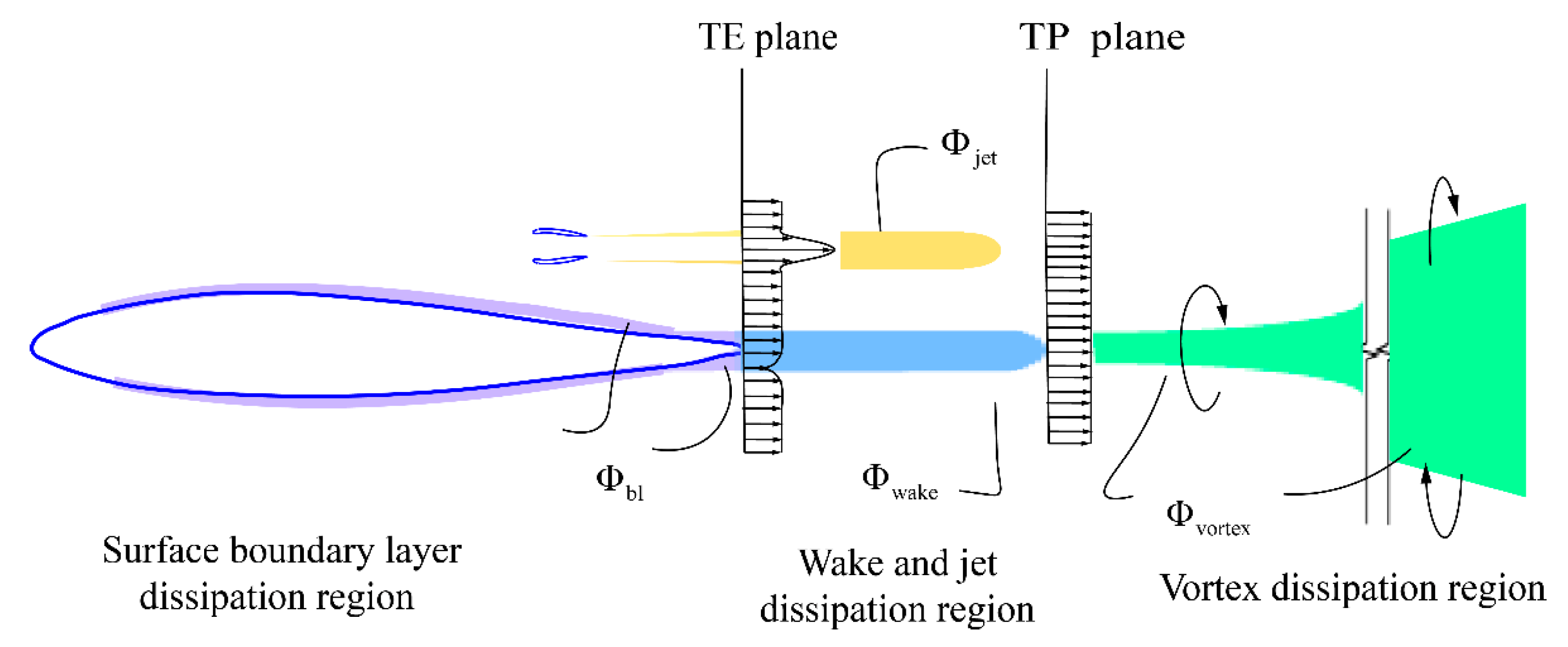
2.2.2. Decomposition of Viscous Dissipation Rate
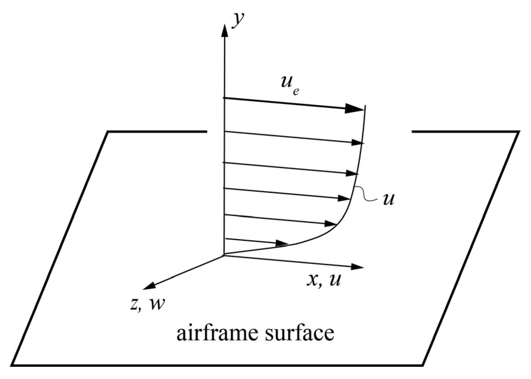
2.2.3. Dissipation Distribution in Boundary Layer and Wake
2.3. CFD Simulation
2.3.1. Solver Setups
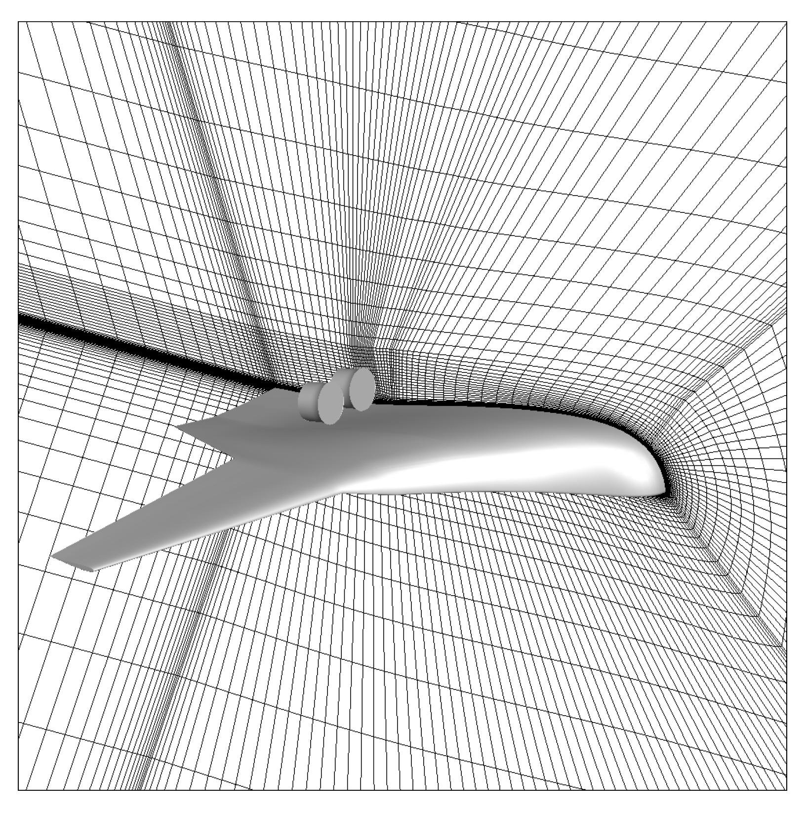
2.3.2. Mesh Setups
2.4. Flight Test
2.4.1. Conditions and Data Collection
2.4.2. Data Postprocessing
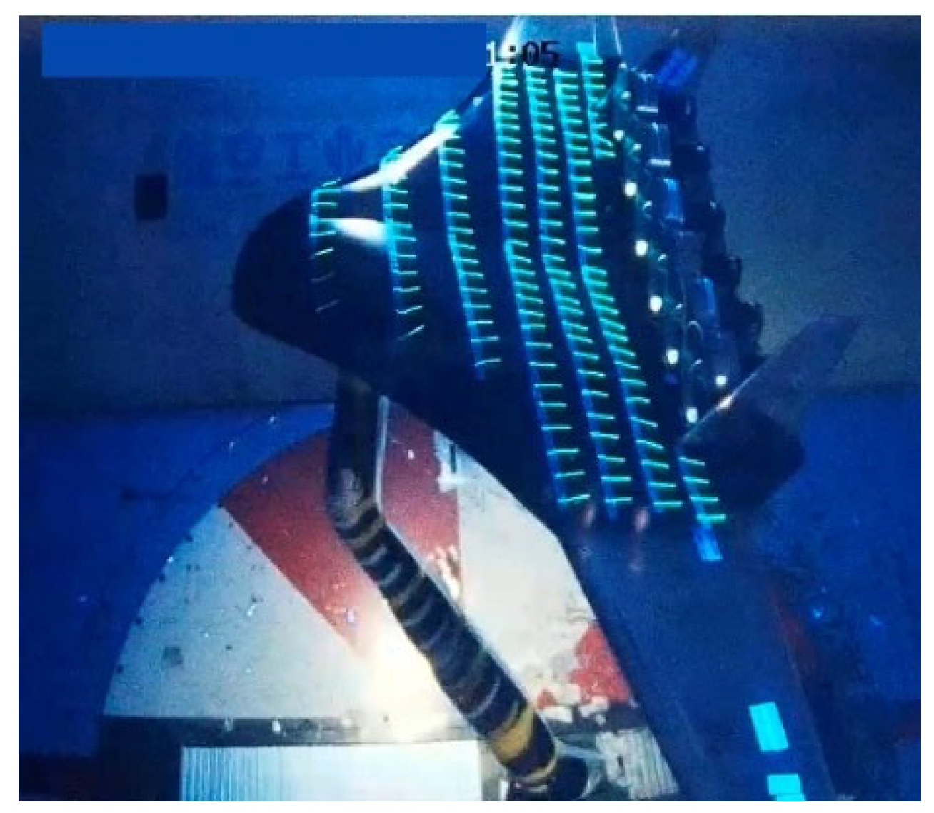
2.4.3. Ground Test for the DP System
2.5. Wind Tunnel Experiments
3. Results and Discussion
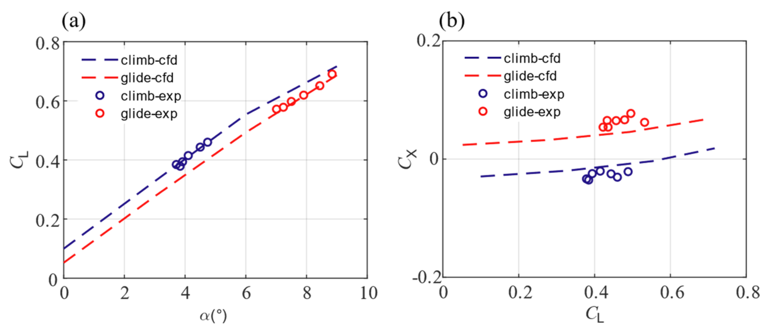
3.1. Impact of DP on the Prestall Aerodynamic Forces of the DPD
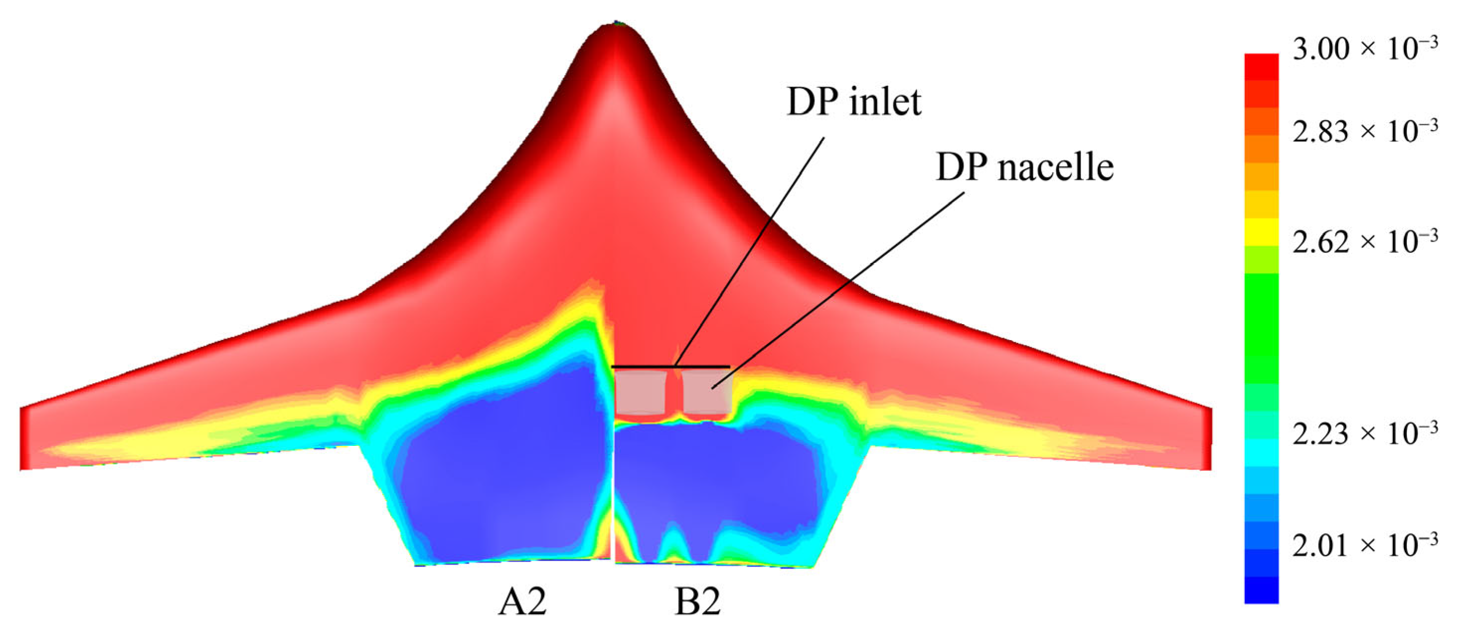
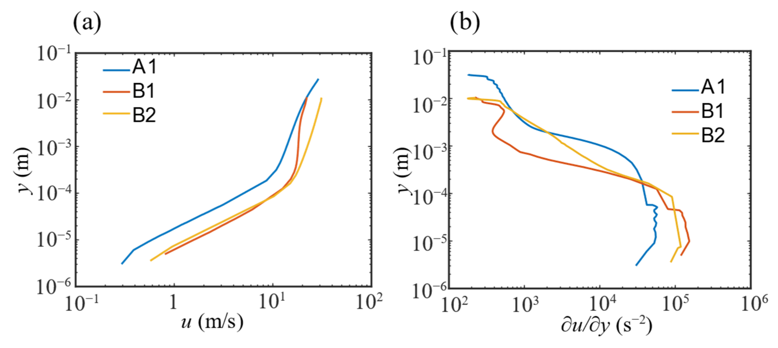
3.2. Impact of the DP System on the Viscous Dissipation Rate of the DPD
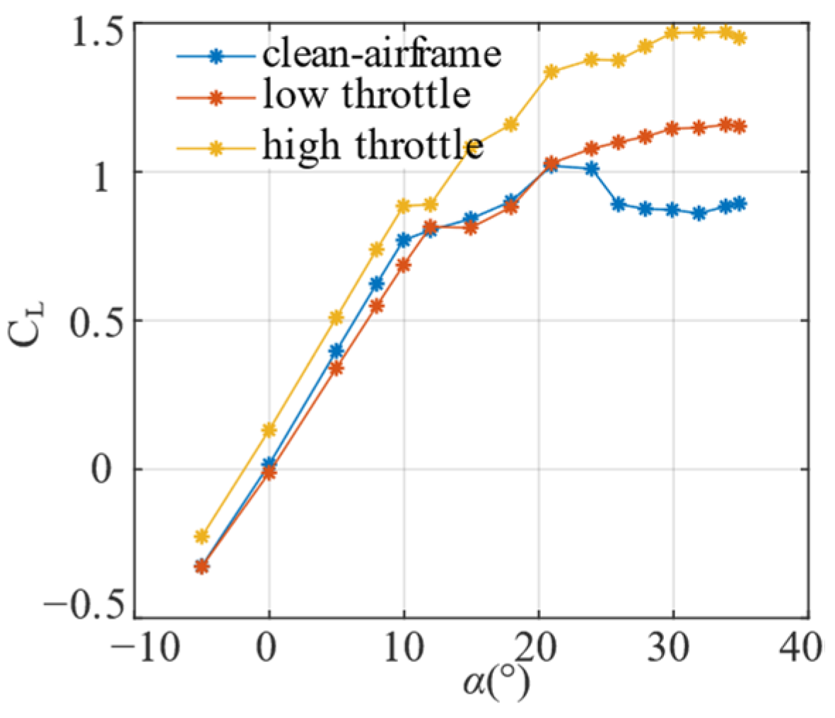
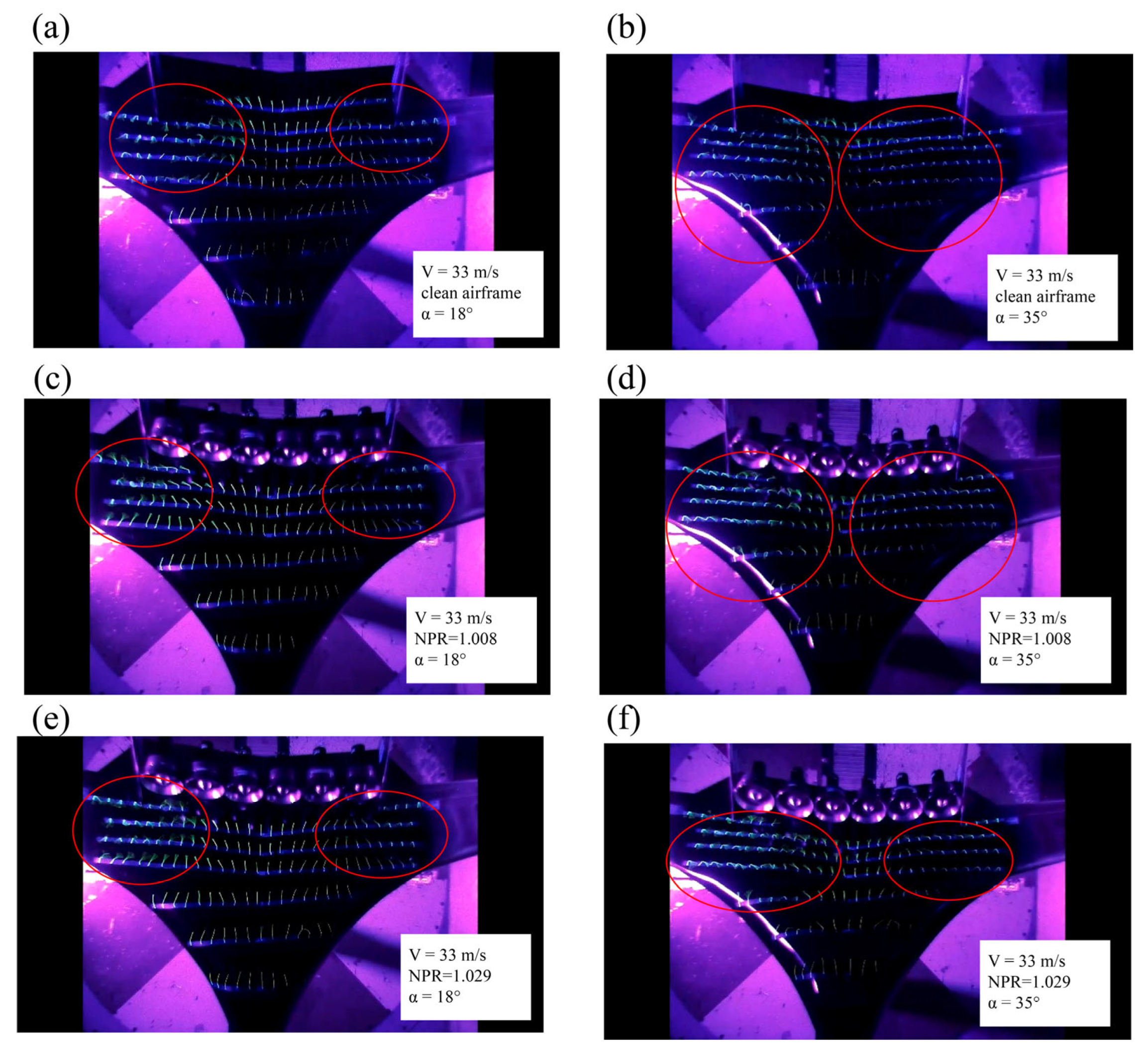
3.3. Improvement of Stall Characteristics of a DPD at Poststall Angles of Attack
4. Conclusions
Author Contributions
Funding
Data Availability Statement
Acknowledgments
Conflicts of Interest
References
- Kim, H.D.; Perry, A.T.; Ansell, P.J. A Review of distributed electric propulsion concepts for air vehicle technology. In Proceedings of the 2018 AIAA/IEEE Electric Aircraft Technologies Symposium, Cincinnati, OH, USA, 12–14 July 2018. [Google Scholar]
- Okonkwo, P.; Smith, H. Review of evolving trends in blended wing body aircraft design. Prog. Aerosp. Sci. 2016, 82, 1–23. [Google Scholar] [CrossRef]
- Brelje, B.J.; Martins, J.R.R.A. Electric, hybrid, and turboelectric fixed-wing aircraft: A review of concepts, models, and design approaches. Prog. Aerosp. Sci. 2019, 104, 1–19. [Google Scholar] [CrossRef]
- Sahoo, S.; Zhao, X.; Kyprianidis, K. A Review of Concepts, Benefits, and Challenges for Future Electrical Propulsion-Based Aircraft. Aerospace 2020, 7, 44. [Google Scholar] [CrossRef] [Green Version]
- Alrashed, M.; Nikolaidis, T.; Pilidis, P.; Jafari, S. Utilisation of turboelectric distribution propulsion in commercial aviation: A review on NASA’s TeDP concept. Chin. J. Aeronaut. 2021, 34, 48–65. [Google Scholar] [CrossRef]
- Hall, C.A.; Crichton, D. Engine Design Studies for a Silent Aircraft. J. Turbomach. 2007, 129, 479–487. [Google Scholar] [CrossRef]
- Felder, J.; Kim, H.; Brown, G. Turboelectric distributed propulsion engine cycle analysis for hybrid-wing-body aircraft. In Proceedings of the 47th AIAA Aerospace Sciences Meeting including The New Horizons Forum and Aerospace Exposition, Orlando, FL, USA, 5–8 January 2009. [Google Scholar]
- Liebeck, R.H. Design of the Blended Wing Body Subsonic Transport. J. Aircr. 2004, 41, 10–25. [Google Scholar] [CrossRef] [Green Version]
- Qin, N.; Vavalle, A.; le Moigne, A.; Laban, M.; Hackett, K.; Weinerfelt, P. Aerodynamic considerations of blended wing body aircraft. Prog. Aerosp. Sci. 2004, 40, 321–343. [Google Scholar] [CrossRef]
- Hileman, J.I.; Spakovszky, Z.S.; Drela, M.; Sargeant, M.A.; Jones, A. Airframe Design for Silent Fuel-Efficient Aircraft. J. Aircr. 2010, 47, 956–969. [Google Scholar] [CrossRef] [Green Version]
- Gohardani, A.S.; Doulgeris, G.; Singh, R. Challenges of future aircraft propulsion: A review of distributed propulsion technology and its potential application for the all electric commercial aircraft. Prog. Aerosp. Sci. 2011, 47, 369–391. [Google Scholar] [CrossRef]
- Kim, H.D.; Felder, J.L.; Tong, M.T.; Armstrong, M. Revolutionary aeropropulsion concept for sustainable aviation: Turboelectric distributed propulsion. In Proceedings of the 2013 International Society for Air Breathing Engines, Busan, Korea, 9–13 September 2013. [Google Scholar]
- Leifsson, L.; Ko, A.; Mason, W.H.; Schetz, J.A.; Grossman, B.; Haftka, R.T. Multidisciplinary design optimization of blended-wing-body transport aircraft with distributed propulsion. Aerosp. Sci. Technol. 2013, 25, 16–28. [Google Scholar] [CrossRef]
- Lv, P.; Rao, A.G.; Ragni, D.; Veldhuis, L. Performance Analysis of Wake and Boundary-Layer Ingestion for Aircraft Design. J. Aircr. 2016, 53, 1517–1526. [Google Scholar] [CrossRef]
- Hall, D.K.; Huang, A.C.; Uranga, A.; Greitzer, E.M.; Drela, M.; Sato, S. Boundary Layer Ingestion Propulsion Benefit for Transport Aircraft. J. Propuls. Power 2017, 33, 1118–1129. [Google Scholar] [CrossRef]
- Uranga, A.; Drela, M.; Greitzer, E.M.; Hall, D.K.; Titchener, N.A.; Lieu, M.K.; Siu, N.M.; Casses, C.; Huang, A.C.; Gatlin, G.M.; et al. Boundary Layer Ingestion Benefit of the D8 Transport Aircraft. AIAA J. 2017, 55, 3693–3708. [Google Scholar] [CrossRef] [Green Version]
- Blumenthal, B.T.; Elmiligui, A.A.; Geiselhart, K.A.; Campbell, R.L.; Maughmer, M.D.; Schmitz, S. Computational Investigation of a Boundary-Layer Ingesting Propulsion System for the Common Research Model. J. Aircr. 2019, 55, 1141–1153. [Google Scholar] [CrossRef] [PubMed]
- Yildirim, A.; Gray, J.S.; Mader, C.A.; Martins, J.R.R.A. Boundary-Layer Ingestion Benefit for the STARC-ABL Concept. J. Aircr. 2022, 59, 896–911. [Google Scholar] [CrossRef]
- Kerho, M.F. Aero-propulsive coupling of an embedded, distributed propulsion system. In Proceedings of the 33rd AIAA Applied Aerodynamics Conference, Dallas, TX, USA, 22–26 June 2015. [Google Scholar]
- Schiltgen, B.T.; Freeman, J. Aeropropulsive interaction and thermal system integration within the ECO-150: A turboelectric distributed propulsion airliner with conventional electric machines. In Proceedings of the 16th AIAA Aviation Technology, Integration, and Operations Conference, Washington, DC, USA, 13–17 June 2016. [Google Scholar]
- Perry, A.T.; Ansell, P.J.; Kerho, M.F. Aero-Propulsive and Propulsor Cross-Coupling Effects on a Distributed Propulsion System. J. Aircr. 2018, 55, 2414–2426. [Google Scholar] [CrossRef]
- Yu, D.; Ansell, P.J.; Hristov, G. Aero-propulsive integration effects of an overwing distributed electric propulsion system. In Proceedings of the AIAA Scitech 2021 Forum, Virtual, 19–21 January 2021. [Google Scholar]
- Borer, N.K.; Derlaga, J.M.; Deere, K.A.; Carter, M.B.; Viken, S.; Patterson, M.D.; Litherland, B.; Stoll, A. Comparison of aero-propulsive performance predictions for distributed propulsion configurations. In Proceedings of the 55th AIAA Aerospace Sciences Meeting, Grapevine, TX, USA, 9–13 January 2017. [Google Scholar]
- Zhang, Y.; Zhou, Z.; Wang, K.; Fan, Z. Influences of distributed propulsion system parameters on aerodynamic characteristics of a BLI-BWB UAV. Xibei Gongye Daxue Xuebao/J. Northwestern Polytech. Univ. 2021, 39, 17–26. [Google Scholar] [CrossRef]
- Zhang, X.; Zhang, W.; Li, W.; Zhang, X.; Lei, T. Experimental research on aero-propulsion coupling characteristics of a distributed electric propulsion aircraft. Chin. J. Aeronaut. 2022; in press. [Google Scholar] [CrossRef]
- Drela, M. Power Balance in Aerodynamic Flows. AIAA J. 2009, 47, 1761–1771. [Google Scholar] [CrossRef] [Green Version]
- Baskaran, P.; Corte, B.D.; van Sluis, M.; Rao, A.G. Aeropropulsive Performance Analysis of Axisymmetric Fuselage Bodies for Boundary-Layer Ingestion Applications. AIAA J. 2022, 60, 1592–1611. [Google Scholar] [CrossRef]


| Parameters | Values |
|---|---|
| Mass, m/kg | 130 |
| Span, b/m | 6.1 |
| Reference area, Sref/m2 | 5.774 |
| Reference length, L/m | 1 |
| Center of gravity, CG/m | 1.31 |
| Aerodynamic center, AC/m | 1.39 |
| Average aerodynamic chord length, c/m | 0.863 |
| Fan length, lfan/m | 0.341 |
| Fan inner diameter, Din/m | 0.241 |
| Fan outer diameter, Dout/m | 0.253 |
| Inlet area, Ain/m | 0.0487 |
| Outlet area, Aout/m | 0.0322 |
| Labels | |
|---|---|
| climb-exp | 0.100 |
| climb-cfd | 0.097 |
| glide-exp | 0.008 |
| glide-cfd | 0.007 |
| α | CX | CPK | |||||
|---|---|---|---|---|---|---|---|
| A1 | 5 | 0.0329 | −0.0020 | 0.0309 | 0.0106 | - | 0.0203 |
| B1 | 5 | 0.0326 | −0.0025 | 0.0301 | 0.0104 | - | 0.0197 |
| A2 | 5 | −0.0145 | 0.0580 | 0.0435 | 0.0109 | 0.0114 | 0.0212 |
| B2 | 4 | −0.0134 | 0.0655 | 0.0521 | 0.0105 | 0.0158 | 0.0258 |
| Φ(x, y) (kg/s3) | 0.5(kg/s3) | Cϕ | |
|---|---|---|---|
| A1 | 46.7 | 1.96 × 10⁴ | 0.0024 |
| B1 | 51.8 | 1.53 × 10⁴ | 0.0034 |
| B2 | 99.7 | 3.23 × 10⁴ | 0.0031 |
Publisher’s Note: MDPI stays neutral with regard to jurisdictional claims in published maps and institutional affiliations. |
© 2022 by the authors. Licensee MDPI, Basel, Switzerland. This article is an open access article distributed under the terms and conditions of the Creative Commons Attribution (CC BY) license (https://creativecommons.org/licenses/by/4.0/).
Share and Cite
Zhao, W.; Zhang, Y.; Tang, P.; Wu, J. The Impact of Distributed Propulsion on the Aerodynamic Characteristics of a Blended-Wing-Body Aircraft. Aerospace 2022, 9, 704. https://doi.org/10.3390/aerospace9110704
Zhao W, Zhang Y, Tang P, Wu J. The Impact of Distributed Propulsion on the Aerodynamic Characteristics of a Blended-Wing-Body Aircraft. Aerospace. 2022; 9(11):704. https://doi.org/10.3390/aerospace9110704
Chicago/Turabian StyleZhao, Wenyuan, Yanlai Zhang, Peng Tang, and Jianghao Wu. 2022. "The Impact of Distributed Propulsion on the Aerodynamic Characteristics of a Blended-Wing-Body Aircraft" Aerospace 9, no. 11: 704. https://doi.org/10.3390/aerospace9110704