Article

Asymptotic Motion of a Satellite under the Action of Sdot Magnetic Attitude Control

Keldysh Institute of Applied Mathematics, Miusskaya Sq. 4, 125047 Moscow, Russia
*
Author to whom correspondence should be addressed.
Aerospace 2022, 9(11), 639; https://doi.org/10.3390/aerospace9110639
Submission received: 9 September 2022 / Revised: 17 October 2022 / Accepted: 21 October 2022 / Published: 24 October 2022
(This article belongs to the Special Issue Spacecraft Attitude Control Using Magnetic Actuators)

Abstract

:
Satellite angular motion under the action of the Sdot one-axis magnetic control algorithm is analyzed. Sdot control stabilizes the maximum moment of inertia axis towards the Sun. Evolutionary equations that avoid singularity in the required position are derived. Linearization of equations is performed and new variables that describe the maximum moment of inertia axis oscillations amplitudes are introduced. The resulting equations are suitable for the averaging method application. Evolutionary equations for slow variables are solved. Simplified evolutionary expressions are verified with numerical simulation.

1. Introduction

An Sdot magnetic attitude control algorithm was proposed in [1]. This one-axis control was designed for the Chibis-M satellite [2] to provide solar panels attitude towards the Sun in emergency situation of the reaction wheels failure. Control was successfully used during the extended mission lifetime in this particular situation [3]. The Sdot control has distinct advantages and disadvantages. As an emergency control algorithm, it benefits from a very simple formulation, thus requiring negligible computation efforts in the commanded dipole moment calculation. Moreover, this control directly utilizes the difference between two consecutive Sun sensor measurements in a way similar to Bdot [4,5], thus avoiding attitude determination routines. The disadvantages are ambiguity in the stabilization direction and low expected accuracy compared to a typical one-axis spin stabilization concept [6,7,8,9,10,11,12,13]. Sdot leads to the satellite rotation. There is no control over the rotation rate since Sun sensors cannot provide information about the rotation around the Sun direction. Sdot may be considered as a simple low performance version of spin stabilization suitable for the Sun’s acquisition in an emergency situation. Similar approach is developed in [14] where Sun sensors and magnetometer measurements are used for the Sun acquisition on a Sun-synchronous orbit. In [15], only two magnetorquers are used. In [16], an intuitive approach is centered around the solar panels’ current output for the control construction. In [17] the Sun direction vector is utilized for the dipole calculation.
The present paper supplements results developed in [1]. Namely, paper [1] analyzes the satellite motion in the Sun acquisition phase, which is far from the required one axis stabilization. Asymptotic behavior is investigated showing that the satellite settles at the rotation around the maximum moment of inertia axis while this axis aligns with the Sun’s direction. However, the equations of motion used in [1] have singularity in the required attitude. Attitude angles of the satellite and its angular momentum that are convenient for the transient motion analysis cannot be used for the investigation of the motion near the required attitude. The present paper fills this gap by introducing different evolutionary equations that are free from singularity in the required attitude. These equations are further linearized and new variables are introduced to represent the amplitudes of oscillations near the Sun’s direction. Linearization is widely used to analyze stability with Floquet theory, design specific magnetic attitude control, or to find an approximate solution to the equations of motion [18,19,20,21,22]. In the present paper, the evolution of amplitudes in linear approximation is investigated using the averaging technique [23,24]. This technique is well suited for the considered problem. The satellite settles at a constant rotation around one axis and the control depends on the periodically varying geomagnetic field. Both situations are extensively studied [25,26,27] with the averaging approach to establish the essential evolutionary dynamics of the satellite. The developed approximate solution is verified with the numerical simulation in the paper.

2. Evolutionary Equations of Motion

Paper [1] utilizes classic evolutionary variables that are also commonly called Beletsky-Chernousko variables [28]. These variables include the angular momentum magnitude and two sets of attitude angles describing the momentum vector and satellite position. Evolutionary equations are convenient for the analysis of spinning satellite dynamics. The rotation rate is characterized by a single variable. A single angle represents the angular momentum vector attitude relative to the designated direction in the inertial space. Similarly, a single nutation angle represents the discrepancy between the angular momentum vector and the maximum moment of the inertia axis. However, the equations exhibit singularity when any of these angles is close to zero. Therefore these equations are well suited for the Sun acquisition motion analysis, but cannot be used in a Sun tracking mode near the required attitude.
To overcome this problem, another set of angles is introduced in the paper. The general approach remains the same. First, the angular momentum vector attitude in the inertial space is established using two angles. Second, the satellite attitude relative to the angular momentum vector is described with three angles. The difference with classic evolutionary variables is that two pairs of angles represent the deviation of the angular momentum from the required direction and the maximum moment of inertia axis deviation from the angular momentum. As a result, this set of angles is less convenient to represent essential motion characteristics, but at the same time the singularity is avoided.

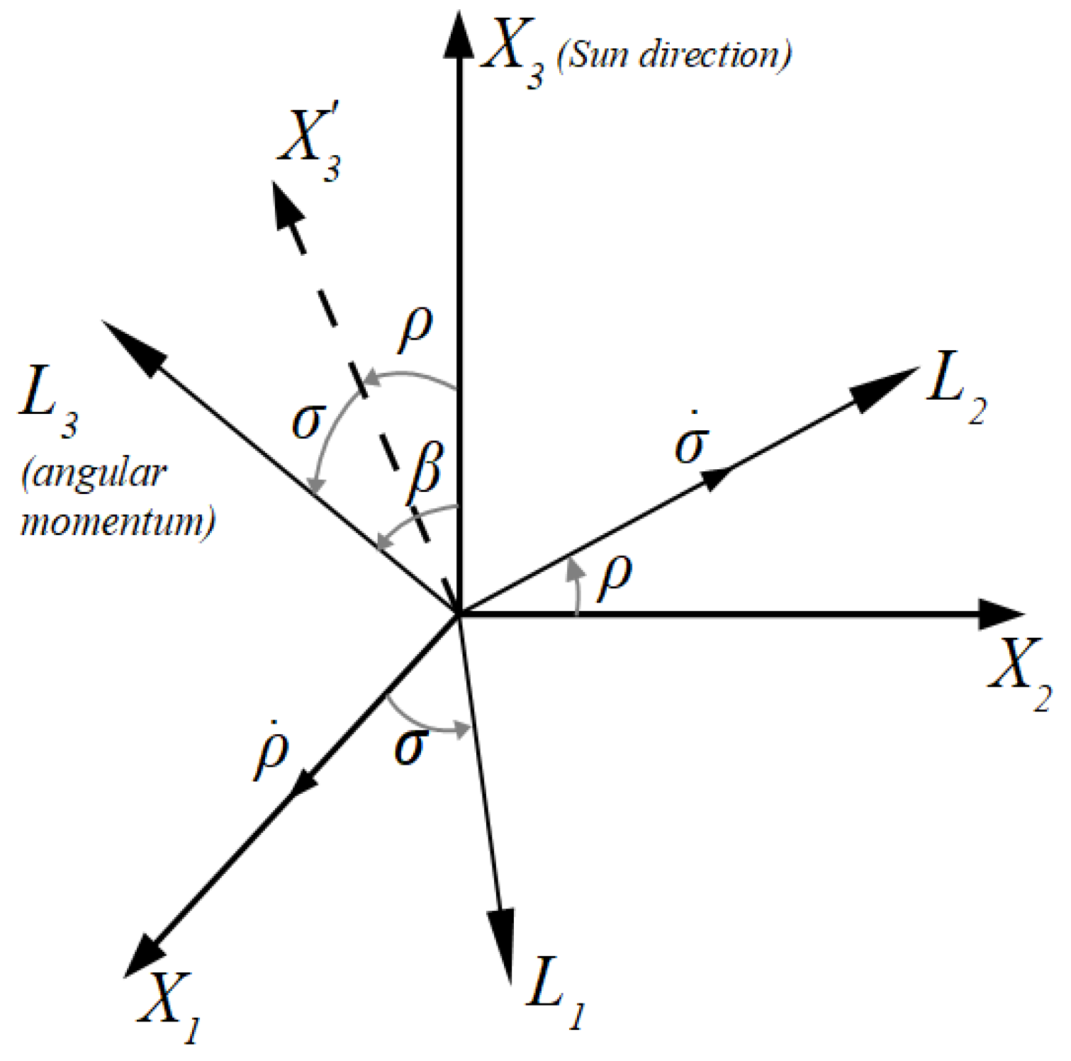
2.1. Angular Momentum Vector Attitude

First the inertial reference frame OY1Y2Y3 is introduced. The origin is placed at the Earth’s center (its motion is neglected on a short time interval of a few hours). Axis OY3 is directed along the satellite orbit normal, and axis OY1 is directed towards the ascending node of a keplerian orbit. This reference frame is used to introduce the geomagnetic induction vector model.
Angular momentum motion is described relative to the inertial reference frame OX1X2X3. This frame has its OX3 axis directed towards the Sun. This direction is considered constant since the dynamic analysis is confined to a few hours and Earth’s motion around the Sun can be neglected. Axes OX1 and OX2 may be chosen at will. Equations of motion utilize satellite attitude with respect to the OX frame whereas the geomagnetic induction vector is represented in the OY frame. Constant matrix C: OYOX is used for the transition between these frames. This matrix depends on the current Sun position OX3 relative to the satellite orbit which is described by OY frame axes.
Reference frame OL1L2L3 is associated with the satellite angular momentum. Axis OL3 is aligned with the momentum vector. The choice of OL1 and OL2 axes is somewhat arbitrary for the single-axis stabilized satellite. In the present paper this choice is governed by the requirement of no singularity in the equations of motion when axes OL3 and OX3 coincide. To construct the OL1 axis, consider the OX1L3 plane (Figure 1). The direction that is perpendicular to OL3 in this plane is designated as OL1. As there are two perpendicular directions in this plane, the angle between OL1 and OX1L3 should be acute for unambiguity of the reference frame construction. Axis OL2 is constructed to complement the right-handed reference frame. The transition from OX reference frame to OL frame is defined by two consecutive rotations. Corresponding angles are defined in Figure 1. The first rotation is performed around the OX1 axis. This rotation aligns OX2 along OL2 axis, and the rotation angle is designated as ρ . A second rotation by the angle σ around the OL2 axis aligns the intermediate third axis with the angular momentum direction OL3. The angle between the angular momentum vector and the maximum moment of inertia axis is defined as cos β = cos θ cos φ .
The required Sun-facing satellite attitude corresponds to the alignment of the angular momentum vector OL3 with the Sun direction OX3 which is characterized by angles ρ = σ = 0 . Unlike classic evolutionary variables, there is no single angle between OL3 and OX3. This complicates the interpretation of the dynamics. On the other hand, this eliminates singularity in the equations of motions. To derive these equations, the transition matrix OLOX is established,
Q = cos σ 0 sin σ sin ρ sin σ cos ρ sin ρ cos σ cos ρ sin σ sin ρ cos ρ cos σ .
Designating the angular momentum vector as L and its magnitude as L one arrives at a simple expression L L = 0 , 0 , L in OL frame. Angular momentum vector in the inertial frame OX is therefore
L X = Q 0 , 0 , L = L sin σ , sin ρ cos σ , cos ρ cos σ .
Subscript X refers to the vector expressed in OX frame. Likewise other subscripts define vectors expressed in different frames further on.
Taking the derivatives of the momentum vector components in the inertial space and solving for L , ρ , and σ derivatives, equations that represent behavior of the angular momentum vector magnitude and its attitude in the inertial space are obtained,
d L d t = M 3 , d ρ d t = 1 L cos σ M 2 , d σ d t = 1 L M 1 ,
where M k are the torque components in the angular momentum reference frame OL in the following analysis.

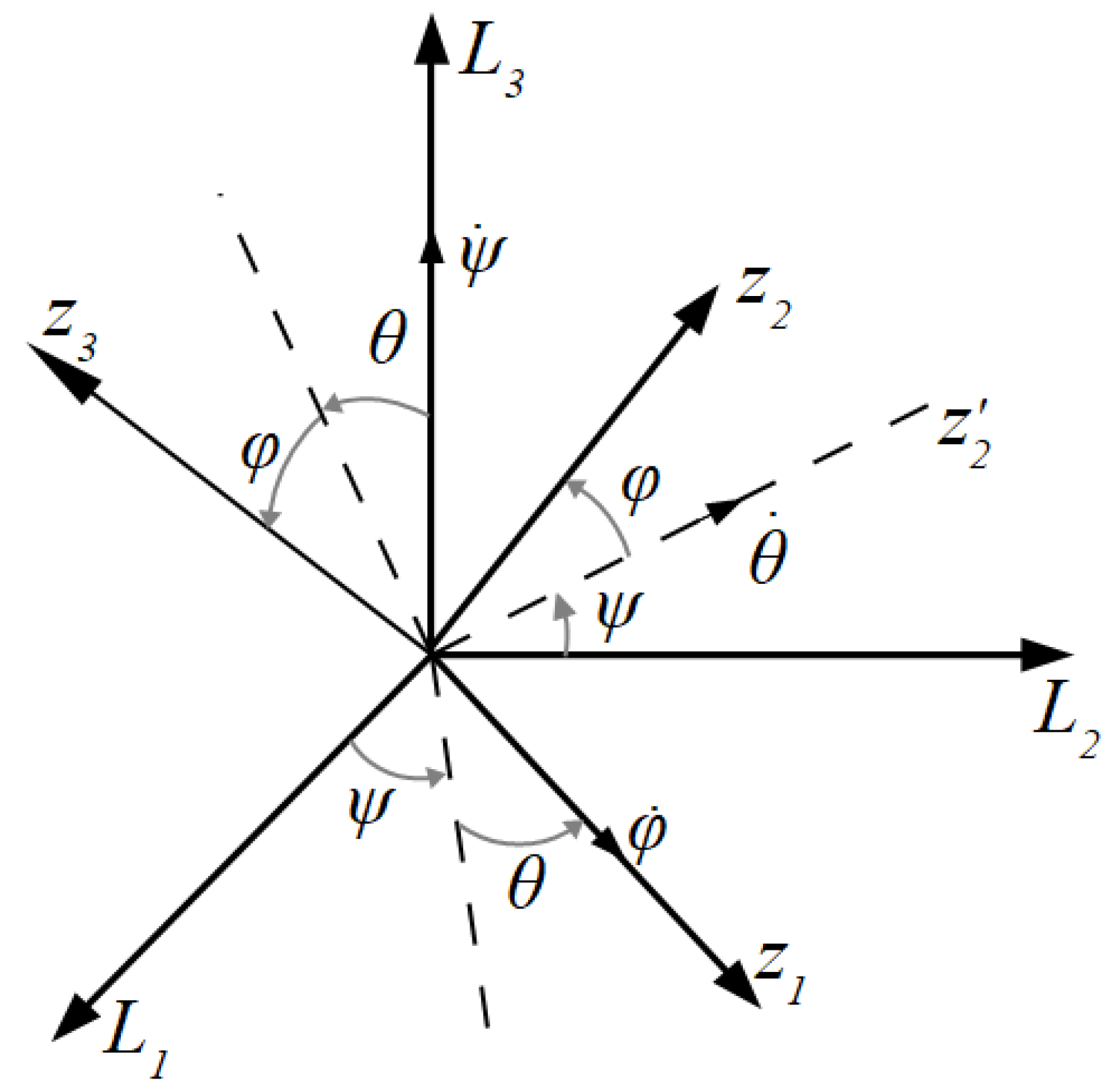
2.2. Satellite Attitude Relative to the Angular Momentum

Satellite-fixed reference frame Oz1z2z3 is defined by the principal central axes of inertia. Satellite reference frame attitude relative to the angular momentum reference frame OL is represented by the rotation angles ψ , θ , φ with rotation sequence 3-2-1 (Figure 2).
The rotation matrix OzOL is
A = cos ψ cos θ sin φ cos ψ sin θ cos φ sin ψ cos φ cos ψ sin θ + sin φ sin ψ sin ψ cos θ sin φ sin ψ sin θ + cos φ cos ψ cos φ sin ψ sin θ sin φ cos ψ sin θ sin φ cos θ cos φ cos θ .
Axis Oz3 is the maximum moment of inertia one further on. As the satellite settles at the rotation around the maximum moment of inertia axis in the Sun acquisition phase [1], this means that Oz3 aligns with OL3. The required attitude is therefore φ = θ = 0 . Analogous to the angular momentum attitude, the maximum moment of inertia axis attitude relative to the angular momentum vector is defined by two angles instead of one in classic evolutionary equations. However, the equations of motion do not exhibit singularity in the required position.
Equations for the attitude angles require expressions for the angular velocity components. Projecting derivatives of angles depicted in Figure 1 and Figure 2 on Oz frame axes yields
ω z 1 = L A a 31 = ψ ˙ a 31 + φ ˙ + ρ ˙ cos σ a 11 + sin σ a 31 + σ ˙ a 21 ,
ω z 2 = L B a 32 = ψ ˙ a 32 + θ ˙ cos φ + ρ ˙ cos σ a 12 + sin σ a 32 + σ ˙ a 22 ,
ω z 3 = L C a 33 = ψ ˙ a 33 θ ˙ sin φ + ρ ˙ cos σ a 13 + sin σ a 33 + σ ˙ a 23 ,
where A , B , C are the principal moments of inertia of the satellite, a i j are matrix A components, ω k are angular velocity components along Oz frame axes. Derivatives of the angular momentum attitude angles ρ , σ are given by (2). Solving equations for the satellite attitude angles derivatives provides
d φ d t = L sin θ 1 A + sin 2 φ B + cos 2 φ C + 1 L cos θ M 1 sin ψ + M 2 cos ψ ,
d ψ d t = L sin 2 φ B + cos 2 φ C + 1 L M 2 cos ψ tan θ + tan σ 1 L M 1 sin ψ tan θ ,
d θ d t = L sin φ cos φ cos θ 1 B 1 C 1 L M 1 cos ψ + M 2 sin ψ .
Equations (2)–(4) fully describe the angular momentum behavior in the inertial space and satellite rotation relative to the angular momentum.

3. Satellite Environment

The satellite motion is considered in two different scenarios. The first simplified scenario is utilized to obtain the approximate evolutionary dynamics of the satellite. It is subjected to the control torque only. Evolutionary equations of motion are solved with an averaging technique revealing expressions that describe the satellite dynamics. In order to verify this result, a second scenario is developed. The satellite is exposed to various disturbance sources in the numerical simulation of initial equations of motion.

3.1. Control Law and Geomagnetic Field Model in Simplified Scenario

The control torque is
M = m × B ,
where m is the control dipole moment, B is the geomagnetic induction vector. Sdot control law expression is [1]
m = k cos α ω × S ,
where k is a positive control gain, S is the direction to the Sun, α is the angle between the Sun direction and geomagnetic induction vector.
The direct dipole model is used for the geomagnetic field representation. The induction vector in OY frame is [29,30]
B Y = B 0 3 2 sin 2 ω 0 t sin i , 3 2 cos 2 ω 0 t 1 2 sin i , cos i = B 0 B 1 Y , B 2 Y , B 3 Y ,
where ω 0 is orbital rate, B 0 = μ / r 3 , μ 7.7245∙106 T∙km3, r is the satellite radius vector.
Note that the induction vector magnitude is not constant. Its magnitude is
B = B 0 χ t ,
where χ t = 1 + 3 sin 2 ω 0 t sin 2 i with i being the orbit inclination. Unit induction vector b Y and its components are introduced according to
b Y = B Y / B 0 χ t ,   b k Y = B k Y / χ .  
Despite not being exactly the induction vector magnitude, constant B 0 is used as a general measure of the field intensity (note that 1 χ 2 ).
Control torque, control dipole moment, and geomagnetic induction expressions complete the dynamical model (2)–(4).

3.2. Satellite Motion Framework in the Numerical Simulation

A numerical simulation is performed with classic Euler angles and quaternion kinematics [31],
J d ω / d t + ω × J ω = M ,
q ˙ 0 q ˙ = 1 2 q 0 q 0 ω ,
where “ ” is the quaternion multiplication and J is the satellite inertia tensor. The satellite is subjected to the control torque, gravitational torque, aerodynamic torque, torque due to the residual dipole moment, and disturbing torque due to the unknown or complex factors.
The control dipole moment (6) is simplified taking into account that d S / d t ω × S for almost constant inertial Sun direction. Further simplifying the derivative as a finite difference, the actual control becomes
m = k cos α S k S k 1 Δ t
where two Sun sensor measurements on two consecutive control steps are used. An IGRF model [32] is used to represent the Earth’s magnetic field for the control torque calculation.
Gravitational torque assumes a central Earth field [31]. Aerodynamic torque is calculated as the sum of torques acting on the sides of a parallelepiped satellite facing the incoming flow [28]. The residual dipole moment has the constant value of the specified magnitude along each satellite axis and periodic part with approximately orbital frequency. Other factors, for example solar radiation pressure, Earth’s oblateness, etc. are generalized under constant and periodic torques, the latter having orbital and double orbital rates. Finally, the Sun’s direction is determined with constant bias and normally distributed noise.

4. Evolutionary Equations near the Required Attitude

Equations of motion (2)-(4) are linearized near the required attitude characterized by small angles φ , θ , ρ , σ ,
d L d t = M 3 , d ρ d t = 1 L M 2 , d σ d t = 1 L M 1 ,
d φ d t = L θ 1 C 1 A + 1 L M 1 sin ψ + M 2 cos ψ ,
d ψ d t = L C + 1 L M 2 θ cos ψ + σ 1 L M 1 θ sin ψ ,
d θ d t = L φ 1 B 1 C 1 L M 1 cos ψ + M 2 sin ψ .
Linearization implies that quantities of the second order of small angles are ignored in the series expansion of cosine function and third order is ignored in sine function. As a result the direction cosines matrices (1) and (3) in the linear approximation become
Q = 1 0 σ 0 1 ρ σ ρ 1 , A = cos ψ sin ψ θ cos ψ + φ sin ψ sin ψ cos ψ θ sin ψ φ cos ψ θ φ 1 .
Specific expressions for the control dipole moment (6) and control torque (5) are required to fully expand equations. Recalling that evolutionary equations utilize torque components in OL frame, the Sun’s direction is calculated as
S L = Q T 0 , 0 , 1 = σ , ρ , 1 .
Note that linearized matrix Q (10) is used. The angular velocity vector in OL frame is related to the velocity vector in Oz frame as ω L = A ω z . The angular momentum vector in Oz frame is related to the angular velocity in the Oz frame and momentum in the OL frame as L z = J ω z = A T 0 , 0 , L . Solving for the velocity in OL frame and using linearized matrix A provides
ω L = L 1 A θ cos ψ 1 B φ sin ψ + 1 C θ cos ψ + φ sin ψ 1 A θ sin ψ + 1 B φ cos ψ + 1 C θ sin ψ φ cos ψ 1 C .
The linearized control dipole moment is therefore
m L = k cos α ω 2 L ρ ω 3 L ω 1 L σ ω 3 L 0 ,
where the angular velocity components ω k L are given by (11). Angle α between the Sun direction and geomagnetic induction vector is calculated in the inertial reference frame. The unit geomagnetic induction vector b X in OX frame is introduced according to (8) as B X = B 0 χ t b X . Specific expressions for the induction vector components are given in the OY frame (7). Transition to the OX frame is performed according to b X = C b Y . Without expanding the transformation expression, b X components are further designated as b k for the majority of the analysis. Note that the subscript “X” that designates vector components in the OX frame is omitted for brevity in b k .
Recalling that the Sun is directed along the OX3 axis and taking into account that b k constitute a unit vector b X , the angle between the Sun direction and the geomagnetic induction vector is calculated as cos α = b 3 . The induction vector in the OL frame is required for the torque calculation,
B L = Q T B X = B 0 χ b 1 σ b 3 b 2 + ρ b 3 b 3 + σ b 1 ρ b 2 .
Substituting the dipole moment and induction vector in the control torque expression (5) provides
M L = k B 0 χ b 3 L σ ω 3 L + ω 1 L b 3 ρ ω 3 L ω 2 L b 3 σ ω 3 L + ω 1 L b 1 ρ ω 3 L ω 2 L b 2 .
Introducing this along with ω k L expressions (11) into the linearized equations of motion yields
d L d t = k B 0 χ b 3 L b 1 1 C σ + θ cos ψ + φ sin ψ 1 A θ cos ψ 1 B φ sin ψ b 2 1 C ρ θ sin ψ + φ cos ψ + 1 A θ sin ψ 1 B φ cos ψ ,
d ρ d t = k B 0 χ b 3 2 1 C ρ + θ sin ψ + φ cos ψ 1 A θ sin ψ + 1 B φ cos ψ ,
d σ d t = k B 0 χ b 3 2 1 C σ + θ cos ψ + φ sin ψ 1 A θ cos ψ 1 B φ sin ψ ,
d φ d t = L θ 1 C 1 A + k B 0 χ b 3 2 1 C σ sin ψ + ρ cos ψ + φ 1 C 1 B ,
d ψ d t = L C ,
d θ d t = L φ 1 B 1 C + k B 0 χ b 3 2 1 C σ cos ψ ρ sin ψ + φ 1 C 1 A .
Note that b k and χ are time-varying and periodic.
Further analysis of the equations of motion requires small parameter introduction and dimensionless time. Angular momentum magnitude L 0 and attitude angles are constant in the absence of the torque. The satellite rotates uniformly in this case,
d ψ d t = L 0 C = c o n s t
The undisturbed rotation rate L 0 / C and corresponding rotation period are used as a base for the dimensionless time τ = L 0 / C t . Small parameter ε = k B 0 / L 0 characterizes the change of the angular momentum relative to its magnitude. The relative change is slow if the control torque is weak enough, and ε 1 . Finally, the dimensionless angular momentum magnitude is expressed in terms of the undisturbed value as l = L / L 0 . Fully dimensionless equations of motion are
l ˙ = ε χ l b 3 b 1 σ + θ cos ψ + φ sin ψ C A θ cos ψ C B φ sin ψ b 2 ρ θ sin ψ + φ cos ψ + C A θ sin ψ C B φ cos ψ ,
ρ ˙ = ε χ b 3 2 ρ + θ sin ψ + φ cos ψ C A θ sin ψ + C B φ cos ψ ,
σ ˙ = ε χ b 3 2 σ + θ cos ψ + φ sin ψ C A θ cos ψ C B φ sin ψ ,
φ ˙ = l θ 1 C A + ε χ b 3 2 σ sin ψ + ρ cos ψ + φ 1 C B ,
ψ ˙ = l ,
θ ˙ = l φ C B 1 + ε χ b 3 2 σ cos ψ ρ sin ψ + φ 1 C A .

5. Linearized Equations Analysis

Equation (12) includes small parameters and therefore l , ρ , and σ are slow variables, whereas the rotation angle ψ is fast. Angles φ and θ represent the maximum moment of inertia axis attitude relative to the angular momentum vector. Intuitively, the angle between the maximum moment of inertia axis and the angular momentum changes slowly. This is formalized in derivatives of φ and θ being proportional to their values, which are small in linear approximation. However, the structure of the equations of motion requires slow variable derivatives to be proportional to small parameter ε for the averaging technique application. Equation (12) does not satisfy this requirement. The additional change of variables is performed to modify these equations.

5.1. Maximum Moment of Inertia Oscillations Amplitude

Angles φ and θ should be replaced with new slow variables. Consider the torque free motion of the satellite for this purpose. In this case ε = 0 and
φ ˙ = λ φ 2 θ , θ ˙ = λ θ 2 φ ,
where λ φ 2 = l C / A 1 , λ θ 2 = l C / B 1 , and the angular momentum magnitude l is constant. Note that C is the maximum moment of inertia. The solution for (13) is
φ = a cos λ φ λ θ τ b λ φ λ θ sin λ φ λ θ τ , θ = a λ θ λ φ sin λ φ λ θ τ + b cos λ φ λ θ τ ,
where a = φ 0 , b = θ 0 .
Torque influence on motion (14) results in change of amplitudes a , b and frequency λ φ λ θ . To find this change, the derivative of the expression for φ is introduced to (12) leading to
φ ˙ = a ˙ cos λ φ λ θ τ a τ d λ φ λ θ d τ sin λ φ λ θ τ a λ φ λ θ sin λ φ λ θ τ b ˙ λ φ λ θ sin λ φ λ θ τ b λ φ λ θ τ d λ φ λ θ d τ cos λ φ λ θ τ b λ φ λ θ cos λ φ λ θ τ = λ φ 2 a λ θ λ φ sin λ φ λ θ τ + b cos λ φ λ θ τ + ε M φ + ε χ b 3 2 1 C B a cos λ φ λ θ τ b λ φ λ θ sin λ φ λ θ τ ,
where M φ = χ b 3 2 σ sin ψ + ρ cos ψ . Note that expressions (14) are used for φ and θ in (12). The frequency derivative is
d λ φ λ θ d τ = d d τ l C / A 1 C / B 1 = ε ξ M l ,
where ξ = C / A 1 C / B 1 , M l is given by the right side of the first equation in (12). Simplifying yields
a ˙ cos λ φ λ θ τ b ˙ λ φ λ θ sin λ φ λ θ τ = ε ξ τ a M l sin λ φ λ θ τ + ε ξ τ b M l λ φ λ θ cos λ φ λ θ τ + ε M φ + ε χ b 3 2 1 C B a cos λ φ λ θ τ b λ φ λ θ sin λ φ λ θ τ .
Performing similar operations with θ provides
a ˙ λ θ λ φ sin λ φ λ θ τ + b ˙ cos λ φ λ θ τ = ε ξ τ a M l λ θ λ φ cos λ φ λ θ τ + ε ξ τ b M l sin λ φ λ θ τ + ε M θ + ε χ b 3 2 1 C A a λ θ λ φ sin λ φ λ θ τ + b cos λ φ λ θ τ ,
where M θ = χ b 3 2 σ cos ψ ρ sin ψ .
Finally solving for the amplitudes derivatives
a ˙ = ε ξ τ b λ φ λ θ M l + ε M a + ε χ a b 3 2 1 C B cos 2 λ φ λ θ τ C A sin 2 λ φ λ θ τ + ε χ b b 3 2 λ φ λ θ C B C A sin λ φ λ θ τ cos λ φ λ θ τ ,
b ˙ = ε ξ τ a M l + ε M b + ε χ b b 3 2 1 C B sin 2 λ φ λ θ τ C A cos 2 λ φ λ θ τ + ε χ a b 3 2 λ θ λ φ C B C A sin λ φ λ θ τ cos λ φ λ θ τ ,
M a = M φ cos λ φ λ θ τ + λ φ λ θ M θ sin λ φ λ θ τ ,
where
M b = λ θ λ φ M φ sin λ φ λ θ τ + M θ cos λ φ λ θ τ .
Unlike derivatives of φ and θ , derivatives of a and b are proportional to the small parameter. Treating (14) as the change of variables φ , θ a , b the equations of motion are represented in the form
l ˙ = ε χ l b 3 b 1 σ + θ cos ψ + φ sin ψ C A θ cos ψ C B φ sin ψ b 2 ρ θ sin ψ + φ cos ψ + C A θ sin ψ C B φ cos ψ ,
ρ ˙ = ε χ b 3 2 ρ + θ sin ψ + φ cos ψ C A θ sin ψ + C B φ cos ψ ,
σ ˙ = ε χ b 3 2 σ + θ cos ψ + φ sin ψ C A θ cos ψ C B φ sin ψ ,
a ˙ = ε ξ τ b λ φ λ θ M l + ε M a + ε χ a b 3 2 1 C B cos 2 λ φ λ θ τ C A sin 2 λ φ λ θ τ +
ε χ b b 3 2 λ φ λ θ C B C A sin λ φ λ θ τ cos λ φ λ θ τ ,
b ˙ = ε ξ τ a M l + ε M b + ε χ b b 3 2 1 C B sin 2 λ φ λ θ τ C A cos 2 λ φ λ θ τ + ε χ a b 3 2 λ θ λ φ C B C A sin λ φ λ θ τ cos λ φ λ θ τ ,
ψ ˙ = l ,
Note that (15) retain φ and θ in the right side of three first equations for brevity. Expression (14) provides relevant dependency φ a , b and θ a , b .

5.2. Averaged Equations of Motion

Equation (15) is suitable for averaging. It contains one fast variable ψ that represents the satellite rotation around the maximum moment of inertia. Slow variables are the angular momentum magnitude, its attitude angles in the inertial space, and the amplitudes of oscillations of the maximum moment of inertia axis relative to the angular momentum vector. Note that Equation (15) also contains time in b k and χ . However, the geomagnetic induction vector changes with the orbital rate. Considering that the satellite rotation rate is significantly higher, Equation (15) is averaged over ψ treating time-dependent terms as slowly varying parameters,
l ˙ = ε χ l b 3 b 1 σ b 2 ρ ,
ρ ˙ = ε χ b 3 2 ρ ,
σ ˙ = ε χ b 3 2 σ ,
a ˙ = ε ξ τ b λ φ λ θ M l + ε χ a b 3 2 1 C B cos 2 λ φ λ θ τ C A sin 2 λ φ λ θ τ +
ε χ b b 3 2 λ φ λ θ C B C A sin λ φ λ θ τ cos λ φ λ θ τ ,
b ˙ = ε ξ τ a M l + ε χ b b 3 2 1 C B sin 2 λ φ λ θ τ C A cos 2 λ φ λ θ τ + ε χ a b 3 2 λ θ λ φ C B C A sin λ φ λ θ τ cos λ φ λ θ τ ,
where M l = χ l b 3 b 1 σ b 2 ρ .
Equations for the angular momentum attitude angles ρ and σ has the form d x / x = f τ d τ and therefore can be directly solved. The exact expression f τ and its integral depend on the geomagnetic induction vector in the OX frame. Recalling from Section 2.1 that B Y = B 0 χ t b Y , B X = C B Y , and expression (7), we arrive at
χ b 3 2 = χ B 3 X χ 2 = 1 χ k = 1 3 m = 1 3 c 3 k c 3 m B k Y B m Y
Here c k m are transition matrix C elements. Induction vector components B k Y are introduced in (7). However, without specifying the Sun’s direction in the OY frame and therefore coefficients c k m it is evident that both angles exponentially tend to zero. The angular momentum magnitude l can be found after ρ and σ directly integrating the first equation in (16). As ρ and σ tend to zero, the angular momentum magnitude tends to the constant value. Overall, the angular momentum vector behavior is fully described by the three first equations in (16), which are independent from the last two equations.

5.3. Maximum Moment of Inertia Oscillations Amplitudes Evolution

The maximum moment of inertia axis motion is described by the last two equations in (16) and expressions (14). Unlike the first three equations in (16), the equations for a and b cannot be directly solved. However, the asymptotic stability of a = b = 0 equilibria can be established. First, we assume that the angular momentum vector already settled near the Sun’s direction, so angles ρ and σ are close to zero and therefore M l 0 . Omitting the first term in equations for a and b provides
a ˙ = ε χ a b 3 2 1 C B cos 2 λ φ λ θ τ C A sin 2 λ φ λ θ τ + ε χ b b 3 2 λ φ λ θ C B C A sin λ φ λ θ τ cos λ φ λ θ τ , b ˙ = ε χ b b 3 2 1 C B sin 2 λ φ λ θ τ C A cos 2 λ φ λ θ τ + ε χ a b 3 2 λ θ λ φ C B C A sin λ φ λ θ τ cos λ φ λ θ τ .
These equations are independent from the equations describing the angular momentum evolution. The following change of variables is introduced,
α = a λ θ λ φ , β = b λ φ λ θ
Equation (18) is expressed as
α ˙ β ˙ = ε χ b 3 2 1 C 2 A C 2 B 1 0 0 1 α β + + 1 2 ε χ b 3 2 C B C A cos 2 λ φ λ θ τ sin 2 λ φ λ θ τ sin 2 λ φ λ θ τ cos 2 λ φ λ θ τ α β .
The next nonsingular change of variables is
α β = cos λ φ λ θ τ sin λ φ λ θ τ sin λ φ λ θ τ cos λ φ λ θ τ u v .
Equation (20) in new variables are
u ˙ v ˙ = ε χ b 3 2 1 C 2 A C 2 B 1 0 0 1 u v + 1 2 ε χ b 3 2 C B C A 1 0 0 1 u v + + λ φ λ θ 0 1 1 0 u v .
The Lyapunov candidate function for this equation is
V = 1 2 u 2 + v 2 .
The derivative of this function is
V ˙ = ε χ b 3 2 1 C B u 2 + ε χ b 3 2 1 C A v 2 .
This derivative is negative if C is the maximum moment of inertia except for the origin u = v = 0 . Therefore, the origin is asymptotically stable. Moreover, as changes of variables (19) and (21) are affine, the initial Equation (18) is stable at origin as well.
Equation (18) may be further simplified by applying averaging over time, thus leading to double averaged equations. Expression χ b 3 2 is expanded according to (17). The induction vector components B k Y , as well as χ , periodically depend on time with frequency η = 2 ω 0 C / L 0 . The averaging of Equation (18) requires right side expansion into a series of trigonometric functions. Therefore, 1 / χ should be expanded. To do so, expression
1 χ 2 = 1 1 + 3 sin 2 1 / 2 η τ sin 2 i = 1 1 + 3 sin 2 i 1 + 2 j = 1 κ 2 j cos j η τ ,
where κ = 1 + 3 sin 2 i 1 3 sin i 2 is established first [33]. Note that parameter κ is relatively small. For example, it is close to ¼ for inclination 51.7°. This parameter is present in powers 2 j in (22). Only the first term in (22) is retained since even this term is noticeably small due to κ 2 0.055 . The root of (22) provides expression for 1 / χ . Decomposing the root in a Tailor series with respect to small parameter κ 2 yields
1 / χ = 1 + 3 sin i 1 / 4 1 + κ 2 cos η τ + O κ 4 .
This expression, as well as expressions (7) for B k Y , are introduced in (18), providing
a ˙ = ε a 1 + 3 sin 2 i 1 / 4 1 + κ 2 cos η τ β 0 + β 1 cos η τ + f T j η τ × 1 C 2 B C 2 A + f T ζ τ + ε b 1 + 3 sin 2 i 1 / 4 1 + κ 2 cos η τ β 0 + β 1 cos η τ + f T j η τ × λ φ λ θ C B C A f T ζ τ , b ˙ = ε b 1 + 3 sin 2 i 1 / 4 1 + κ 2 cos η τ β 0 + β 1 cos η τ + f T j η τ × 1 C 2 B C 2 A + f T ζ τ + ε a 1 + 3 sin 2 i 1 / 4 1 + κ 2 cos η τ β 0 + β 1 cos η τ + f T j η τ × λ θ λ φ C B C A f T ζ τ .
Here j = 1 , 2 , ζ = λ φ λ θ , f T are trigonometric functions, parameters
β 0 = α 0 2 + 1 / 2 α 1 2 + 1 / 2 α 2 2 ,
β 1 = 2 α 0 α 1 ,
α 0 = c 33 cos i 1 / 2 c 32 sin i ,
α 1 = 3 / 2 c 31 sin i ,
α 2 = 3 / 2 c 32 sin i
are derived from (7).
Functions f T j η τ , f T ζ τ , as well as their products with cos η τ , are zero on average provided that ζ and η are incommensurable. Therefore the double averaged equations are
a ˙ = ε 1 + 3 sin 2 i 1 / 4 β 0 + 1 2 κ 2 β 1 1 C 2 B C 2 A a , b ˙ = ε 1 + 3 sin 2 i 1 / 4 β 0 + 1 2 κ 2 β 1 1 C 2 B C 2 A b .
These equations are independent. They are directly solved revealing the exponential decay of the maximum moment of inertia axis oscillations amplitudes.

6. Numerical Simulation

Two numerical simulation scenarios are utilized. The first one corresponds to the simplified framework summarized in Section 3.1 and is used throughout the motion analysis. The goal of this simulation is to verify simplifications adopted in the analysis methodology, which is linearization of the equations of motion and their subsequent single or double averaging. A second simulation scenario is based on the framework of Section 3.2 and includes disturbance sources. This verifies the applicability of developed approximate results to the realistic formulation of satellite motion.

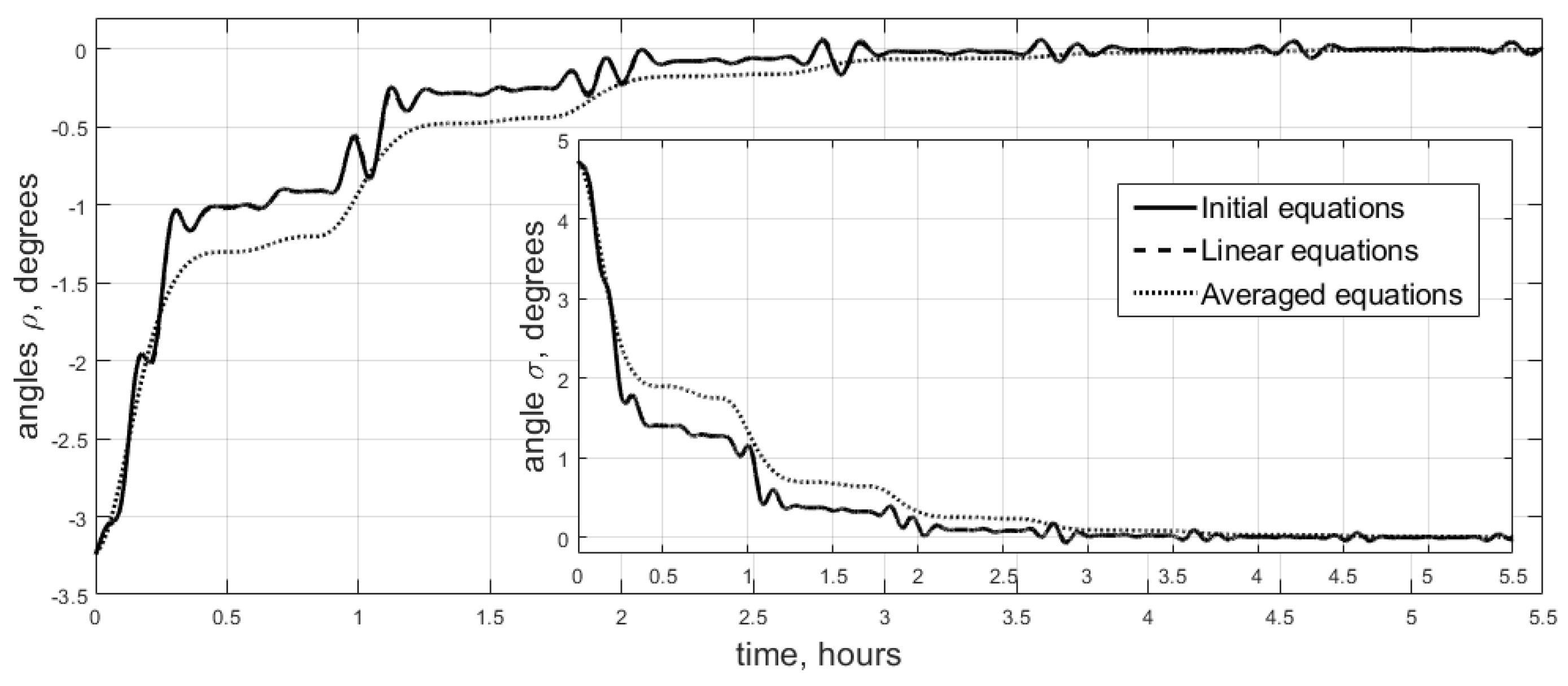
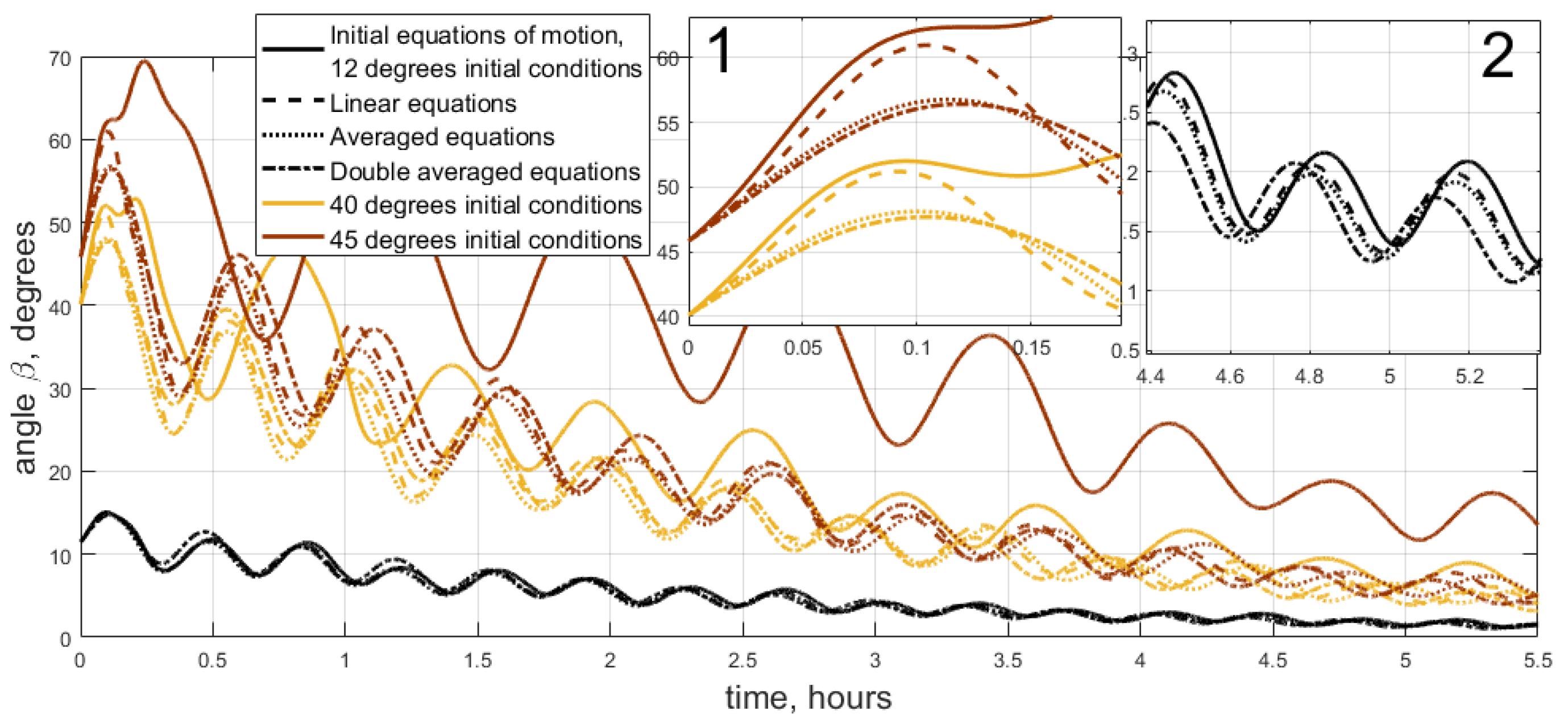
6.1. Simplified Scenario Simulation

Independent simulations of initial evolutionary Equations (2)-(4), linear Equation (15), averaged Equation (16), and double averaged Equation (23) are performed. The following parameters are utilized:
  • Inertia moments of the satellite 1.1, 1.3, 1.5 kg·m2;
  • Orbit inclination 51.7°, altitude 550 km (derived parameters are B 0 ≈ 24,000 nT, orbital rate ω 0 ≈ 10−3 s−1);
  • The Sun’s direction in reference frame OY is defined by two angles, ρ S and σ S , equal to 50 degrees each. These angles are introduced similarly to the angular momentum vector attitude angles ρ and σ in Section 2.1, Figure 1. Accordingly, expression (1) is used for the transition matrix C calculation;
  • Control gain k = 60 kg·m2/s·T.
One of the simplifications utilized in the motion analysis is linearization of the equations of motion. Attitude matrices Q and A are linearized as well in (10). However, unlike initial proper transition matrices, the linearized matrices are no longer orthonormal. Therefore, each time a transition between the reference frame is performed the transformed vector is slightly “stretched”. Typically, this does not lead to noticeable errors since the variables tend to zero in linear approximation anyway. In this paper one of the variables is the angular momentum magnitude which is essentially non-zero in terminal motion. Instead, it settles at a constant magnitude. This magnitude differs in linear and nonlinear equations due to the stretching of the momentum vector in linear approximation. The difference does not exceed the overall accuracy of the linearization assumption. However, the difference may be reduced by adjusting the initial angular momentum magnitude. Namely, the initial momentum magnitude is set to be identical in the inertial reference frame OX in linear and initial equations of motion. Using nonlinear momentum as a base one, recalling transformation rule L X = Q L L , and momentum expression in OL frame L L 0 = 0 , 0 , L 0 , the relation between initial conditions becomes
L l i n e a r 0 = L n o n l i n e a r 0 / q k 3 = L n o n l i n e a r 0 / 1 + σ 2 0 + ρ 2 0 ,
where matrix Q elements q k 3 are calculated in linear approximation. Another adjustment of initial conditions is sometimes required for the averaged equations of motion. Initial and averaged variables are generally not equal at t = 0 , and the averaging procedure is in fact a change of variables. However, in the present case this adjustment turned out to be unnecessary while requiring relatively bulky calculations.
Moving to the simulation results, Figure 3 provides the angular momentum magnitude. Note that the angular momentum behavior is fully covered by the first three averaged equations in (16). It does not depend on the motion of the maximum moment of inertia axis oscillations. Therefore, the angular momentum behavior is the same for averaged and double averaged equations and the latter are not present in Figure 3 and Figure 4.
The angular momentum magnitude remains almost constant according to Figure 3. The satellite motion in the paper is considered near the required attitude, so it is close to the required rotation and mainly wobble suppression is performed. The difference between the averaged and initial equation may seem considerable in Figure 3. However, this difference doesn’t exceed ε 2 , which is the general averaging method accuracy.
Angular momentum attitude angles are provided in Figure 4.
Figure 4 indicates good accuracy of averaged equations in describing the angular momentum evolutionary motion.
Oscillations of the maximum moment of inertia axis relative to the angular momentum vector are revealed with Figure 5. Note that initial equations of motion (2)–(4) are absent in Figure 5 since they lack the oscillations amplitudes and operate with original attitude angles φ and θ instead.
Figure 5 indicates that the simplest double averaged Equation (23) may be used to analyze satellite dynamics relative to the angular momentum vector. Equation (23) and expressions (14) allow angle β between the angular momentum and the maximum moment of inertia axis (see Figure 1) calculation for the initial nonlinear equations of motion. Figure 6 presents a comparison of this angle in four simulation scenarios.
Figure 6 presents simulation results for different initial conditions. This was performed to assess the range of applicability of the linearization assumption. Close-up №2 in Figure 6 indicates that the approximate amplitudes derived from (23)–(14) provide very accurate prediction of the satellite maximum moment of inertia axis motion for small attitude angles up to 15 degrees. The accuracy is fairly accurate up to 30 degrees and linear approximation loses its applicability at about 40 degrees deviation. Close-up № 1 shows this situation. It is clearly seen that linear equations of motion diverge significantly from the nonlinear very quickly. Together with the angular momentum behavior reported in Figure 4, Figure 6 provides overall confirmation of the applicability of the analysis method and the results adopted in Section 4 and Section 5.

6.2. Simulation in a Realistic Scenario

Simplified results are further verified with the simulation of satellite motion with various disturbance sources outlined in Section 3.2. The following parameters are used:
  • aerodynamic torque calculation:
  • satellite parallelepiped sides are 0.2, 1.1, 1.8 m. This is a simplified geometry of Chibis-M satellite which was equipped with solar panels;
  • center of mass displacement relative to the center of pressure is 4, 6, 8 cm along satellite frame axes;
  • atmosphere density is 1.8 × 10⁻¹³ kg/m3 which corresponds to average solar activity for 550 km orbit;
  • residual dipole moment value is approximately 2 × 10⁻³ A·m2. This corresponds to its possible estimation accuracy [34,35,36];
  • Sun direction determination error is 1 degree, both for the constant bias and noise;
  • unknown disturbance value is approximately half of the gravitational torque;
  • control torque calculation and numerical integration steps are one second each;
  • orbit is slightly elliptical with eccentricity 0.01.
The simulation result is provided in Figure 7 for the angle between the maximum moment of inertia axis and the Sun’s direction.
Figure 7 indicates that averaged equations of motion adequately describe satellite dynamics near the required attitude. Note that disturbance parameters strongly affect this fact. For example, aerodynamic torque may have a lot higher magnitude during maximum solar activity. Doubling its magnitude significantly reduces the quality of the approximate result compared to the numerical simulation. Clearly, the higher that the disturbances magnitude is, the less is the accuracy of no-disturbance dynamics analysis. Extensive numerical simulation of satellite motion under Sdot control with significant disturbances influence is present in [37].

7. Conclusions

Satellite motion in the Sun tracking mode is investigated. An Sdot magnetic attitude control algorithm is utilized. Equations of motion suitable for the analysis of satellite motion near the required attitude are derived. Satellite dynamics is analyzed in linear approximation with an averaging technique. Simplified equations of motion that can be directly integrated are obtained. Attitude evolution towards the required motion is described with an accuracy of less than a degree if initial deviation is in the linear range. Simplified results are tested against the numerical simulation results for the satellite dynamics with various disturbance sources showing an accuracy of a few degrees and the overall successful prediction of satellite evolutionary motion.

Author Contributions

Conceptualization, M.O. and D.R.; methodology, D.R.; software, S.T.; formal analysis, D.R.; writing—original draft preparation, D.R.; writing—review and editing, S.T. and M.O. All authors have read and agreed to the published version of the manuscript.

Funding

This research received no external funding.

Data Availability Statement

Not applicable.

Conflicts of Interest

The authors declare that they have no conflicts of interest.

References

  1. Karpenko, S.; Ovchinnikov, M.; Roldugin, D.; Tkachev, S. One-axis attitude of arbitrary satellite using magnetorquers only. Cosm. Res. 2013, 51, 478–484. [Google Scholar] [CrossRef]
  2. Zelenyi, L.; Gurevich, A.; Klimov, S.; Angarov, V.; Batanov, O.; Bogomolov, A.; Bogomolov, V.; Bodnar, L.; Vavilov, D.; Vladimirova, G.; et al. The academic Chibis-M microsatellite. Cosm. Res. 2014, 52, 87–98. [Google Scholar] [CrossRef]
  3. Ovchinnikov, M.; Roldugin, D.; Tkachev, S.; Karpenko, S. New one-axis one-sensor magnetic attitude control theoretical and in-flight performance. Acta Astronaut. 2014, 105, 12–16. [Google Scholar] [CrossRef]
  4. Stickler, A.C. A Magnetic Control System for Attitude Acquisition; NASA-CR-130145; NTRS: Washington, DC, USA, 1972. [Google Scholar]
  5. Stickler, A.; Alfriend, K. Elementary Magnetic Attitude Control System. J. Spacecr. Rocket. 1976, 13, 282–287. [Google Scholar] [CrossRef]
  6. Shigehara, M. Geomagnetic attitude control of an axisymmetric spinning satellite. J. Spacecr. Rocket. 1972, 9, 391–398. [Google Scholar] [CrossRef]
  7. Thomson, W. Spin stabilization of attitude against gravity torque. J. Astronaut. Sci. 1962, 9, 31–33. [Google Scholar]
  8. Zavoli, A.; Giulietti, F.; Avanzini, G.; De Matteis, G. Spacecraft Dynamics Under the Action of Y-dot Magnetic Control Law. Acta Astronaut. 2016, 122, 146–158. [Google Scholar] [CrossRef] [Green Version]
  9. Avanzini, G.; de Angelis, E.; Giulietti, F. Spin-axis pointing of a magnetically actuated spacecraft. Acta Astronaut. 2014, 94, 493–501. [Google Scholar] [CrossRef]
  10. de Ruiter, A. A fault-tolerant magnetic spin stabilizing controller for the JC2Sat-FF mission. Acta Astronaut. 2011, 68, 160–171. [Google Scholar] [CrossRef]
  11. Wheeler, P. Spinning Spacecraft Attitude Control via the Environmental Magnetic Field. J. Spacecr. Rocket. 1967, 4, 1631–1637. [Google Scholar] [CrossRef]
  12. Soken, H.; Sakai, S.; Asamura, K.; Nakamura, Y.; Takashima, T.; Shinohara, I. Filtering-Based Three-Axis Attitude Determination Package for Spinning Spacecraft: Preliminary Results with Arase. Aerospace 2020, 7, 97. [Google Scholar] [CrossRef]
  13. Aleksandrov, A.; Tikhonov, A. Monoaxial Electrodynamic Stabilization of an Artificial Earth Satellite in the Orbital Coordinate System via Control With Distributed Delay. IEEE Access 2021, 9, 132623–132630. [Google Scholar] [CrossRef]
  14. You, H.; Jan, Y. Sun Pointing Attitude Control with Magnetic Torquers Only. In Proceedings of the 57th International Astronautical Congress, Valenica, Spain, 2–6 October 2006; p. IAC-06-C1.2.01. [Google Scholar]
  15. Jan, Y.; Tsai, J.-R. Active control for initial attitude acquisition using magnetic torquers. Acta Astronaut. 2005, 57, 754–759. [Google Scholar] [CrossRef]
  16. Kim, J.; Worrall, K. Sun tracking controller for UKube-1 using magnetic torquer only. IFAC Proc. Vol. 2013, 46, 541–546. [Google Scholar] [CrossRef]
  17. Ignatov, A.; Sazonov, V. Stabilization of the Solar Orientation Mode of an Artificial Earth Satellite by an Electromagnetic Control System. Cosm. Res. 2018, 56, 388–399. [Google Scholar] [CrossRef]
  18. Morozov, V.; Kalenova, V. Stabilization of Satellite Relative Equilibrium Using Magnetic Moments and Aerodynamic Forces. Cosm. Res. 2022, 60, 213–219. [Google Scholar] [CrossRef]
  19. Ergin, E.; Wheeler, P. Magnetic attitude control of a spinning satellite. J. Spacecr. Rocket. 1965, 2, 846–850. [Google Scholar] [CrossRef]
  20. Sorensen, J. A Magnetic Attitude Control System for an Axisymmetric Spinning Spacecraft. J. Spacecr. Rocket. 1971, 8, 441–448. [Google Scholar] [CrossRef]
  21. Zhou, B. Lyapunov differential equations and inequalities for stability and stabilization of linear time-varying systems. Automatica 2021, 131, 109785. [Google Scholar] [CrossRef]
  22. Malkin, I. Theory of Stability of Motion; U.S. Atomic Energy Commission, Technical Information Service: Oak Ridge, TN, USA, 1952. [Google Scholar]
  23. Arnold, V.; Kozlov, V.; Neishtadt, A. Dynamical Systems III: Mathematical Aspects of Classical and Celestial Mechanics; Springer: Berlin/Heidelberg, Germany, 2007. [Google Scholar]
  24. Bogoliubov, Y.; Mitropolsky, N. Asymptotic Methods in the Theory of Nonlinear Oscillations; Gordon and Breach: Philadelphia, PA, USA, 1961; ISBN 067720051X. [Google Scholar]
  25. Celani, F. Robust three-axis attitude stabilization for inertial pointing spacecraft using magnetorquers. Acta Astronaut. 2015, 107, 87–96. [Google Scholar] [CrossRef] [Green Version]
  26. Benson, C.; Scheeres, D. Averaged Solar Torque Rotational Dynamics for Defunct Satellites. J. Guid. Control. Dyn. 2021, 44, 749–766. [Google Scholar] [CrossRef]
  27. Aleksandrov, A.; Tikhonov, A. Averaging technique in the problem of Lorentz attitude stabilization of an Earth-pointing satellite. Aerosp. Sci. Technol. 2020, 104, 105963. [Google Scholar] [CrossRef]
  28. Beletsky, V. Motion of an Artificial Satellite about Its Center of Mass; Israel Program for Scientific Translation: Jerusalem, Israel, 1966. [Google Scholar]
  29. Ovchinnikov, M.; Penkov, V.; Roldugin, D.; Pichuzhkina, A. Geomagnetic field models for satellite angular motion studies. Acta Astronaut. 2018, 144, 171–180. [Google Scholar] [CrossRef]
  30. Antipov, K.; Tikhonov, A. Multipole models of the geomagnetic field: Construction of the Nth approximation. Geomagn. Aeron. 2013, 53, 257–267. [Google Scholar] [CrossRef]
  31. Wertz, J. Spacecraft Attitude Determination and Control; Springer: Dordrecht, Netherlands, 1990. [Google Scholar]
  32. Alken, P.; Thébault, E.; Beggan, C.; Amit, H.; Aubert, J.; Baerenzung, J.; Bondar, T.; Brown, W.; Califf, S.; Chambodut, A.; et al. International Geomagnetic Reference Field: The thirteenth generation. Earth Planets Space 2021, 73, 49. [Google Scholar] [CrossRef]
  33. Ovchinnikov, M.; Roldugin, D. Magnetic attitude control and periodic motion for the in-orbit rotation of a dual-spin satellite. Acta Astronaut. 2021, 186, 203–210. [Google Scholar] [CrossRef]
  34. Inamori, T.; Sako, N.; Nakasuka, S. Compensation of time-variable magnetic moments for a precise attitude control in nano- and micro-satellite missions. Adv. Space Res. 2011, 48, 432–440. [Google Scholar] [CrossRef]
  35. Inamori, T.; Sako, N.; Nakasuka, S. Magnetic dipole moment estimation and compensation for an accurate attitude control in nano-satellite missions. Acta Astronaut. 2011, 68, 2038–2046. [Google Scholar] [CrossRef]
  36. Busch, S.; Bangert, P.; Dombrovski, S.; Schilling, K. UWE-3, in-orbit performance and lessons learned of a modular and flexible satellite bus for future pico-satellite formations. Acta Astronaut. 2015, 117, 73–89. [Google Scholar] [CrossRef]
  37. Roldugin, D.; Tkachev, S.; Ovchinnikov, M. Satellite Angular Motion under the Action of SDOT Magnetic One Axis Sun Acquisition Algorithm. Cosm. Res. 2021, 59, 529–536. [Google Scholar] [CrossRef]
Figure 1. Angular momentum vector attitude in the inertial space.
Aerospace 09 00639 g001
Figure 2. Satellite attitude relative to the angular momentum.
Aerospace 09 00639 g002
Figure 3. Angular momentum magnitude.
Aerospace 09 00639 g003
Figure 4. Angular momentum attitude angles.
Aerospace 09 00639 g004
Figure 5. Satellite oscillations amplitudes relative to the angular momentum.
Aerospace 09 00639 g005
Figure 6. Angle between the angular momentum and maximum moment of inertia axis.
Aerospace 09 00639 g006
Figure 7. Solar panels attitude relative to the Sun.
Aerospace 09 00639 g007
Publisher’s Note: MDPI stays neutral with regard to jurisdictional claims in published maps and institutional affiliations.

