Article

Dynamic Modeling and Analysis of Thrust Reverser Mechanism Considering Clearance Joints and Flexible Component

1
School of Mechanical Engineering and Automation, Northeastern University, Shenyang 110819, China
2
AECC Shenyang Engine Research Institute, Shenyang 110015, China
*
Author to whom correspondence should be addressed.
Aerospace 2022, 9(10), 611; https://doi.org/10.3390/aerospace9100611
Submission received: 5 September 2022 / Revised: 30 September 2022 / Accepted: 12 October 2022 / Published: 17 October 2022

Abstract

:
As a high-precision motion mechanism, the kinematics and dynamics of cascade thrust reverser are sensitive to the changes of nonlinear factors which are rarely considered in traditional dynamic modeling and optimization. In order to study the effect of nonlinear factors on the dynamics behavior of cascade thrust reverser mechanism, the dynamic model considering joint clearance and flexible component is established. Lankarani–Nikravesh and modified-Coulomb model are used to establish the contact force at the clearance, and the flexible component in the mechanism is modeled by the absolute node coordinate method. The effects of joint clearance value, clearance position, flexible component, and driving speed on the dynamic response of the mechanism are studied. Specifically, the nonlinear characteristics of the mechanism increase with the clearance value, and the joint clearance near the mobile fairing has greater influence on the kinematics and dynamics of blocker door. For the mechanical system with clearances, the flexible component can partially reduce the vibration of the system. The analysis of the motion synchronization of the thrust reverser actuators indicates that the asynchronous movement of actuators may increase the driving forces of actuators especially for the middle actuator.

1. Introduction

The reverse thrust device is used to change the thrust direction of the engine, which can decelerate and shorten the landing distance after the aircraft touches the ground. Compared with braking, spoiler, and other deceleration modes, the reverse thrust device is not limited by rain, snow, and other weather conditions, and can reduce the wear of brake pads with good braking effect and high safety factor, so it is widely used in turbojet and turbofan engines of civil and military aircrafts [1,2,3,4,5]. The thrust reverser structure mainly includes bucket type, lobe type, and cascade type. Among them, the cascade type thrust reverser has high thrust reverser efficiency, high reliability, and strong adaptability to different engine conditions. Therefore, it is widely used in large bypass ratio turbofan engine. Each mobile fairing of the cascade thrust reverser is usually driven by three actuators which are powered by hydraulic pressure. A synchronous soft shaft is installed inside the hydraulic pipeline in order to adjust the speed of different actuators, so as to ensure the synchronous movement of actuators during the deployment and retraction process of the thrust reverse device. When the reverse thrust device is in operation during the landing process, the mobile fairing moves backward and drives the blocker doors to turnover, which can change the direction of bypass airstream to generate reverse thrust force and realize the deceleration effect of the aircraft [6,7,8,9,10].
The research on the cascade thrust reverser mainly focuses on aerodynamic performance [11,12,13,14,15,16,17], loading system design [18,19,20], structural parameter optimization design [21]. V. L. Varsegov, et al. [17] studied the numerical model of the airflow through thrust reverser in the engine bypass duct, and proposed the optimal turbulence model. J. Butterfield, et al. [20] focused on the design of the cascade of the thrust reverser and analyzed the pressure distribution on the section of the thrust reverser. E. W. M. Roosenboom [22] successfully measured the flow field of thrust reversal by three-dimensional particle image velocimetry technology, and obtained the influence of blade position on aerodynamic performance. S. Zhang et al. [13] obtained the load-bearing and force transmission characteristics of the thrust reverser mechanism. K. L. McCormick et al. [23] studied the working performance of the thrust reverser by comparing the deceleration effect of the thrust reverser with the braking equipment.
Most of the studies in the above-mentioned literatures are based on the idealized rigid body model, and mainly studied the influence of the thrust flow field on the bearing capacity and working performance of the whole mechanism. In addition, some researchers have studied the kinematics, dynamics, and structural optimization of the mechanism based on traditional single degree of freedom thrust reverser mechanism [5,12,21]. However, there is little research on the current two-degree-of-freedom (DOF) thrust reverser mechanism. Compared with traditional mechanisms, the motion of the 2-DOF thrust reverser mechanism is more complex, and the mechanism dynamics is more sensitive to nonlinear factors [24]. Therefore, it is necessary to study the influence of nonlinear factors on mechanism dynamics. At the same time, as a driving device, the synchronization of the thrust reverser actuator directly affects the change of the driving force of the mechanism, and the synchronization of the actuator has become an important problem in the design and analysis of the mechanism.
In this paper, the cascade thrust reverser is taken as the research object. On the basis of the structural analysis of the thrust reverser, the kinematic and dynamic models of the single chain thrust reverser are established. Based on the single chain model, the influence of nonlinear factors such as joint clearance and flexible component on the dynamics of the thrust reverser are studied, and the effect of thrust reverser actuators synchronization on mechanism dynamics is analyzed through spatial multi-link model.

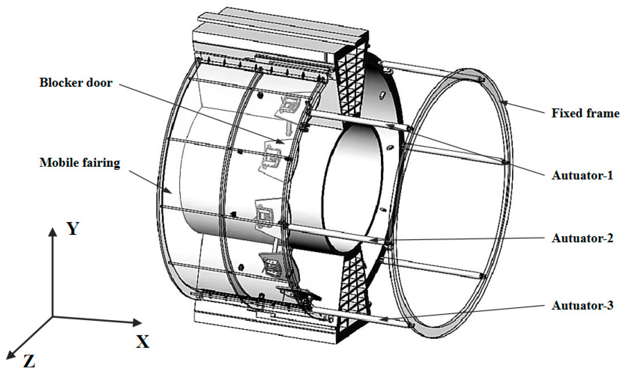
2. Thrust Reverser Mechanism

The cascade thrust reverser is mainly composed of mobile fairing, blocker door, pull rod of blocker door, exhaust cascade, and reverse thrust actuator, etc. In order to facilitate the kinematic and dynamic analysis of the cascade thrust reverser, the schematic diagram of a typical cascade thrust reverser is extracted as shown in Figure 1.
In order to ensure sufficient exhaust area of the cascade, a transfer pull rod is added between the blocker door and the large pull rod, which makes the reverse thrust device a two degree of freedom mechanism with only one input. In order to ensure the under actuated mechanism having a unique motion law, a torsion spring and a limit lug are installed.
The three actuators extend under the hydraulic power to drive the mobile fairing along the air flow direction and open the thrust reverser. In order to ensure the synchronous movement of the thrust reverser actuators, a synchronous soft shaft is connected between each actuator, and the soft shaft is connected with the piston of the actuator through a worm gear mechanism. During the deployment or retraction of the thrust reverser device, the displacement difference between the actuators caused by the inconsistent aerodynamic loads would generate synchronous torque of soft shaft to adjust the actuators and realize the synchronous movement of the thrust reverser device.

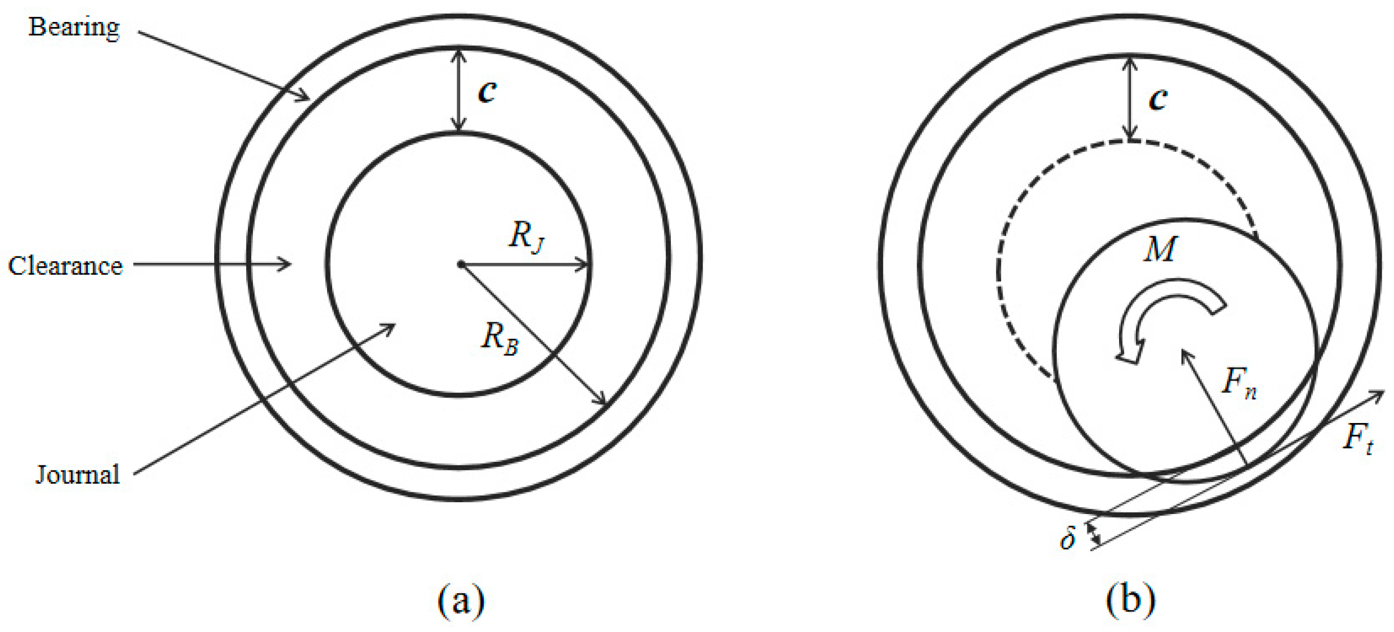
3. Modeling of Revolute Joint with Clearance

In order to analyze the dynamic characteristics of multi-body mechanism with joint clearance, a contact collision model between journal and bearing was established. Figure 2 shows the model diagram of the joint clearance in two states.
The clearance value c can be expressed by the difference between the bearing diameter R B and the journal diameter R J .
c = R B R J
When the center offset distance between the journal and the bearing is less than the clearance value c, the journal and bearing are in a free flight state, otherwise the journal and bearing are in the contact deformation state. The contact force includes normal contact force and tangential friction force. In addition, the tangential friction force will also generate a rotational moment M.

3.1. Normal Contact Force Model

Lankarani et al. [25] proposed the Lankarani–Nikravesh contact force model which estimates the damping factor η by the kinetic energy loss during the collision, which can be expressed as follows:
F n = K δ n + D δ ˙
K = 4 3 ( σ i + σ j ) ( R i R j R i + R j ) 1 2
σ k = 1 μ k 2 E k ,   ( k = i , j )
D = 3 K ( 1 C e 2 ) δ n 4 δ ˙ *
F n = K δ n [ 1 + 3 K ( 1 C e 2 ) δ ˙ 4 δ ˙ * ]
where δ is the contact deformation, N represents the contact force index,   E i and E j represent the elastic modulus of the shaft and the bearing respectively, μ i and μ j represent Poisson’s ratio of shaft and bearing respectively. C e is the recovery coefficient, δ ˙ * is the relative velocity at the initial time of contact.
The L-N contact force model can accurately simulate the contact and collision process at the clearance, and is widely used in the dynamic analysis of mechanisms with clearance [26,27,28,29]. In this paper, L-N contact force model is used to calculate the normal contact force at the clearance.

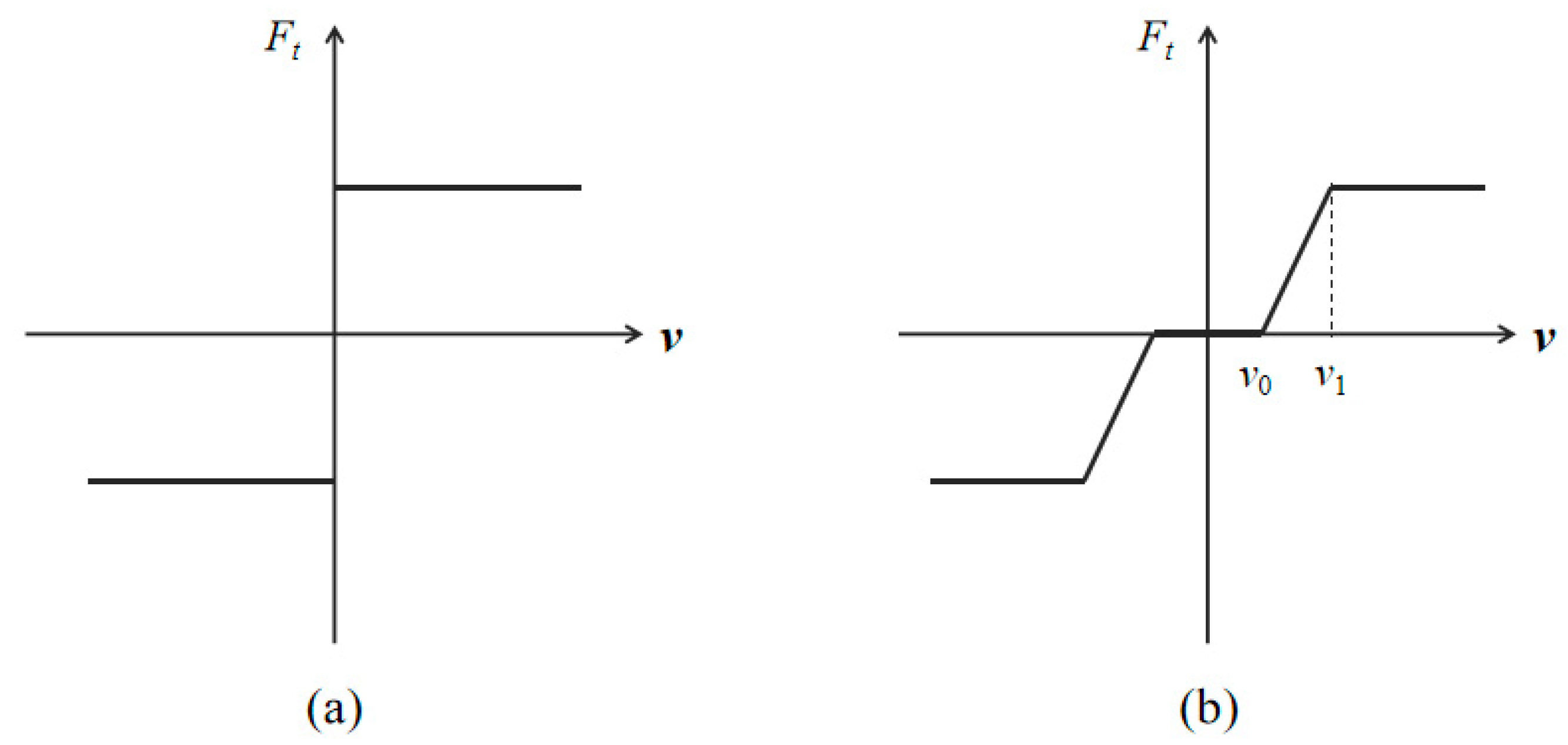
3.2. Tangential Friction Force Model

Coulomb friction model is the most typical friction model [30], in which, the friction force is proportional to the normal contact force
F t = μ | F n | sgn ( v )
where, F t is the tangential friction force, μ is the friction coefficient, v is the relative motion speed.
However, as shown in Figure 3a, when the motion speed is zero, the friction force is discontinuous, and results in non-convergence problem.
The modified Coulomb friction model proposed by Ambrosio [31] is more reasonable, which introduces a transition state around the zero velocity.
F t = c f c d F n v t | v t |
c d = { 0 | v t | v 0 v 1 v 0 1 if   | v t | < v 0 if   v 0 < | v t | < v 1 if   | v t | > v 1
where c f is the friction coefficient, v t is the relative speed, c d is the dynamic correction coefficient, v 0 and v 1 are the speed values specified for calculating the dynamic correction coefficient. The modified Coulomb friction model is used to calculate the tangential friction force in this paper.

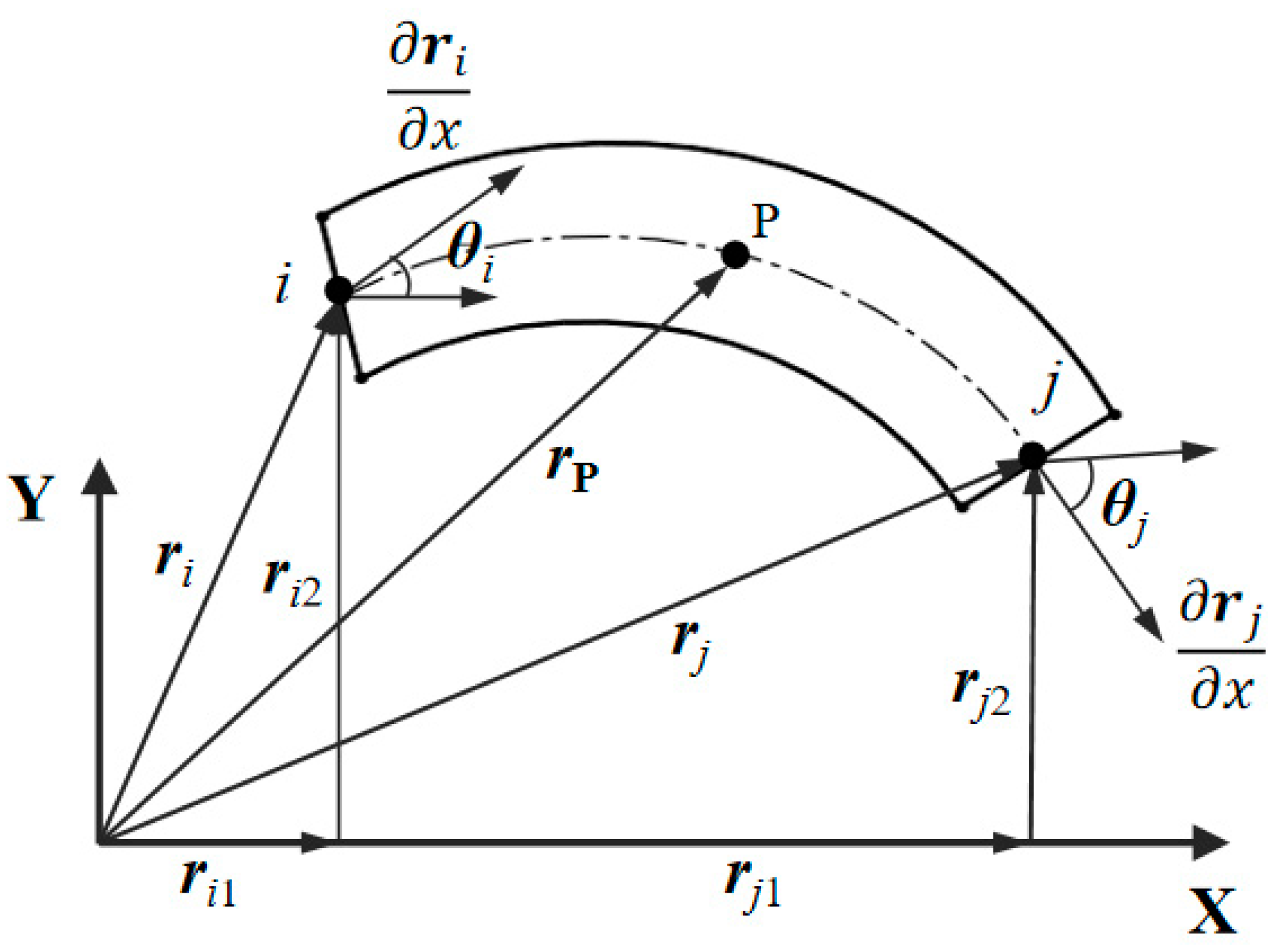
4. Modeling of Revolute Joint with Clearance

The flexible beam element is modeled by absolute nodal coordinate formulation (ANCF) [32,33], as shown in Figure 4.
In the global coordinate system, the position vector of any point P on the flexible beam element can be expressed as
r = [ r x r y ] = [ a 0 + a 1 x + a 2 x 2 + a 3 x 3 b 0 + b 1 x + b 2 x 2 + b 3 x 3 ] = S q e
q e = ( q 1 , q 2 , q 3 , q 4 , q 5 , q 6 , q 7 , q 8 ) T = ( r i x , r i y , r i x x , r i y x , r j x , r j y , r j x x , r j y x ) T
where, S is the global shape function, q is the generalized coordinate of the flexible beam element, [ r m x , r m y ] T ( m = i , j ) represents the position vector of nodes i, j, [ r m x x , r m y x ] T represents the absolute position slope of the beam element node in the global coordinate system.
The global shape function s of the flexible beam element can be expressed as
S = ( S 1 I , S 2 I , S 3 I , S 4 I )
where, I is the identity matrix of 2 × 2, S 1 = 1 3 ξ 2 + 2 ξ 3 , S 2 = l ( ξ 2 ξ 2 + ξ 3 ) , S 3 = 3 ξ 2 2 ξ 3 , S 4 = l ( ξ 3 ξ 2 ) , ξ = x / l , l is the length of flexible beam element.
The kinetic energy of the beam element can be expressed as
T = 1 2 0 V ρ r ˙ T r ˙ d V = 1 2 q e ˙ T ( 0 V ρ S T S d V ) q e ˙ = 1 2 q e ˙ T M a q e ˙
where, M a is the mass matrix of the flexible beam element, ρ and V are the density and volume of the flexible beam element.
Taking the derivative of strain energy with respect to the generalized coordinate, the elastic force of flexible beam element can be written as:
Q k = U e
where Q k is the elastic force of the flexible beam element, U is the total strain energy.
The longitudinal strain energy U l and bending strain energy U t of the beam element can be expressed as:
U l = 1 2 0 l E A ε l 2 d x
U t = 1 2 0 l E I e κ 2 d x
where I e is moment of inertia of the element cross section. κ is the curvature of the beam element.
The total strain energy U consists of U l and U t , can be expressed as:
U = U l + U t = 1 2 0 l ( E A ε l 2 + E I e κ 2 ) d x
Longitudinal elastic force Q l and bending elastic force Q t can be expressed as:
Q l = ( U l e ) T = [ 0 l E A ε l ( S T S ) d x ] e = K l e
Q t = ( U t e ) T = [ 0 l E I ( S T S ) d x ] e = K t e
where, K l is the stiffness matrix corresponding to the longitudinal elastic force, K t is the stiffness matrix corresponding to the bending elastic force.
The total elastic force Q k and total stiffness matrix K of the beam element can be written as
Q k = Q l + Q t = [ 0 l E A ε l ( S T S ) d x ] e + [ 0 l E I ( S T S ) d x ] e
K = K l + K t = 0 l E A ε l ( S T S ) d x + 0 l E I ( S T S ) d x

5. Dynamic Equation of Rigid-Flexible Coupling Mechanism with Joint Clearance

According to Lagrange multiplier method, the dynamic equation of multi-body system with clearances can be expressed as:
{ M a q ¨ + Φ q T λ = Q a Q k + F c Φ ( q , t ) = 0                                                            
where q , q ˙ , and q ¨ are the generalized coordinate, velocity, and acceleration of the system, λ is the Lagrange multiplier matrix, Q a is the generalized external force of the system. Fc is the contact force at the clearance. Φ ( q , t ) is the constraint equation, Φ q is the Jacobian matrix of the constraint equation.
Φ q = Φ ( q , t ) q
Because the mechanism includes rigid body and flexible body simultaneously, the mass matrix and generalized coordinate of the mechanism can be written as follows:
M = [ M r 0 0 M f ] , q = [ q r q f ]
where index r and f represent rigid body and flexible body, respectively.
According to the above equation, the dynamic equation of rigid-flexible coupling multi-body system with clearances can be written as:
{ [ M r 0 0 M f ] [ q r q f ] + [ Φ q r T Φ q f T ] λ = [ Q r Q f ] Φ ( q r , q f , t ) = 0
In order to facilitate numerical algorithm design and calculation, the dynamic equation can be written as:
[ M a Φ e T Φ e 0 ] [ q ¨ λ ] = [ Q γ 2 α Φ ˙ β 2 Φ ]
γ = Φ q q ¨ = ( Φ q q ˙ ) q q ˙ 2 Φ qt q ˙ Φ tt
where Q is the generalized force matrix, α and β are Baumgarte correction coefficients. γ represents the acceleration constraint equation of the mechanism.

6. Calculation and Parameters

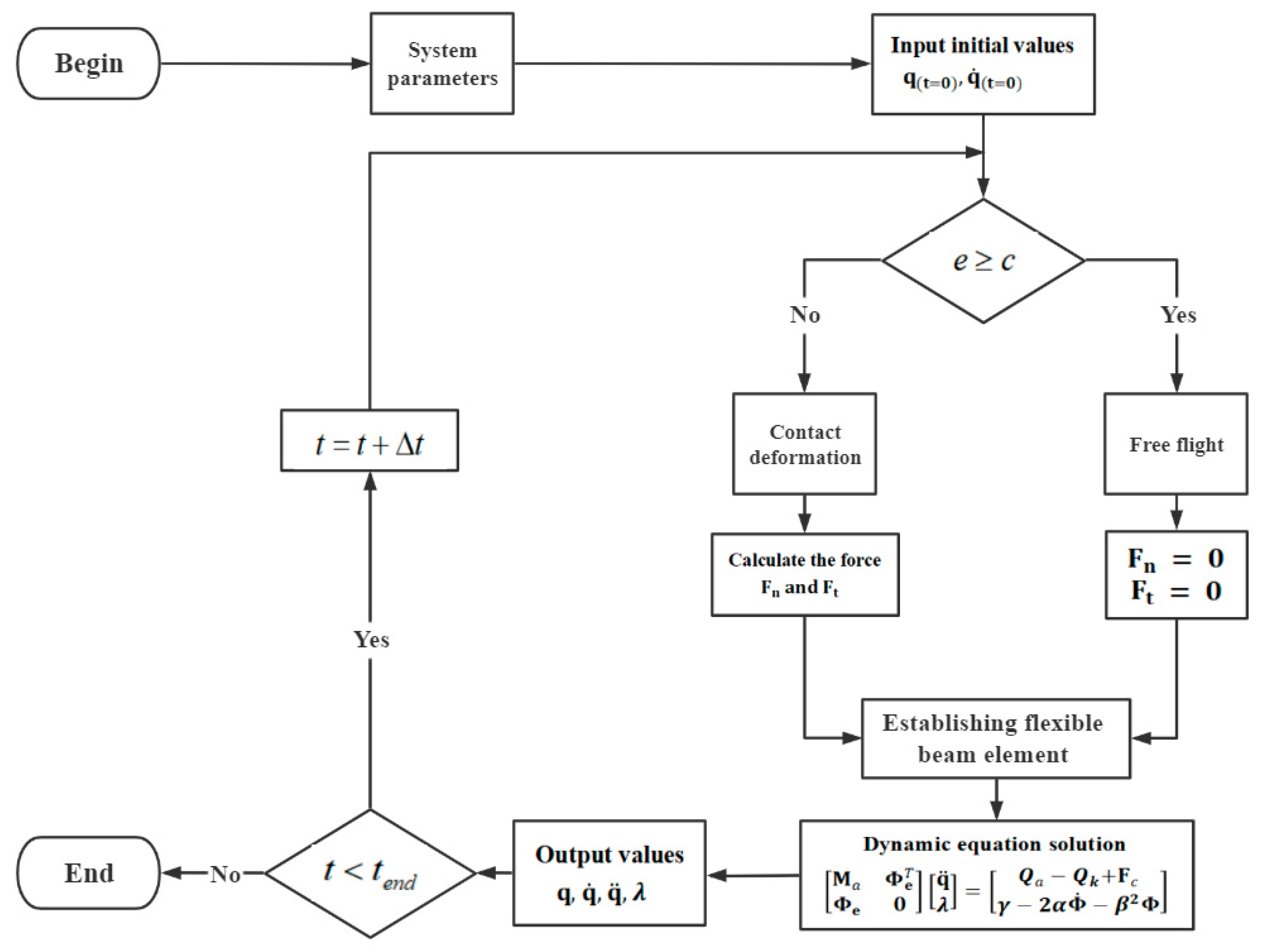
6.1. Solution Process of Dynamic Equation

The dynamic equation of the system is a differential equation containing strongly coupled characteristics and strongly nonlinear characteristics. In order to improve the calculation accuracy and reduce the error, the fourth-order Runge-Kutta method is used to solve DAEs of the system in this paper. The flowchart of solving the dynamic equation is shown in Figure 5, and the solution procedures are as follows: (1) Enter the system parameters and define initial condition, including position coordinates and speed; (2) determine whether the shaft and bearing are in collision, and calculate the contact force; (3) establish the flexible beam element model and obtain the elastic force; (4) calculate the generalized coordinates and velocity by solving the differential algebra dynamic equations; (5) repeat (2)(3)(4) until the end time.

6.2. Model Validation

In order to verify the accuracy of the established model, take the classical three-dimensional flexible pendulum in the literature [34] as an example for comparison. The flexible pendulum is under gravity with initial angular velocity about the vertical Y-axis. The flexible pendulum model diagram is shown in Figure 6, and Table 1 shows the model simulation parameters.
Figure 7 shows the comparison between the calculated results of the established model and the literature results, it can be seen that the two results are highly consistent, which verifies the accuracy of the established model in this paper.

6.3. Mechanism Simulation Parameters

The structural parameters of thrust reverse mechanism are shown in Table 2, the simulation parameters of clearance collision are shown in Table 3, and the simulation parameters of flexible component are shown in Table 4.

7. Results and Discussion

7.1. Dynamic Response Analysis of the Mechanism

7.1.1. Effect of Clearance Value

This section analyzes the effect of different clearance values on dynamic response and nonlinear characteristics of mechanism. Clearance joints A and B are considered simultaneously in the mechanism with the clearance values of 0.1 mm, 0.3 mm, and 0.5 mm respectively under constant driving speed of 0.5 m/s. When the blocker door enters the overturning stage, the aerodynamic load gradually increases from 0 to 2000 N, as shown in Figure 8. The displacement, velocity, and acceleration of blocker door, the driving force and the reaction force of clearance joint are shown in Figure 9. The phase diagrams and Poincare maps of clearance joints A and B are represented in Figure 10.
It can be seen from Figure 9a that the displacement of block door under different clearance values are basically the same, while velocity and acceleration fluctuate more dramatically with larger clearance, which indicates that clearance may worsen the stability of the mechanism. The driving forces of different clearance are identical and maximum driving forces of different clearance all appear at 0.95 s, which is due to the aerodynamic load, but the fluctuation of driving force becomes more obvious with the increase of the clearance value. Figure 9e shows that the contact force at clearance joint A decreases as the clearance value increases. While the maximum contact force at clearance joint B is less influenced by clearance compared with A. From the above kinematics and dynamics curves, it can be found that with the increase of the aerodynamic load on the blocker door, the fluctuation caused by the joint clearance is significantly weakened.
According to Figure 10, with the increase of clearance value, the range of phase diagram further expands and the mapping points from Poincare diagram are less concentrated, which indicates that the periodicity of the motion at the clearance is stronger with smaller clearance, and the nonlinearity of the motion increases with the clearance value. Compared with clearance A, the motion at clearance B is more chaotic.

7.1.2. Effect of the Positions of Clearance Joint

This section analyzes the effect of different positions of clearance joint on dynamic response and nonlinear characteristics of mechanism, the clearance of 0.3 mm is added to joint A and B separately. The kinematic characteristics of blocker door and the driving force are calculated with driving speed of 0.5 m/s. The kinematics of blocker door and the driving force of mechanism are shown in Figure 11. The shaft center trajectory and phase diagram at clearance A and B are shown in Figure 12. Figure 13 shows the phase diagram of blocker door movement with clearance joint A and B, respectively.
It can be seen that the displacement with different locations of clearance joint are basically the same. The fluctuation of velocity, acceleration, and driving force caused by clearance joint B is larger than clearance joint A. It is noteworthy that there is sudden change at around 0.3 s, which is due to the overturning of blocker door. Compared with clearance joint A, the clearance joint B has greater impact on the movement of block door.
It can be seen that under the same clearance value, the movement range of the shaft center at the clearance B is larger and the nonlinear characteristics are stronger. The range of phase diagram of blocker door under the effect of clearance joint A is smaller than that of clearance B and the motion of blocker door under clearance joint A is more stable, which can be verified by the relative acceleration.

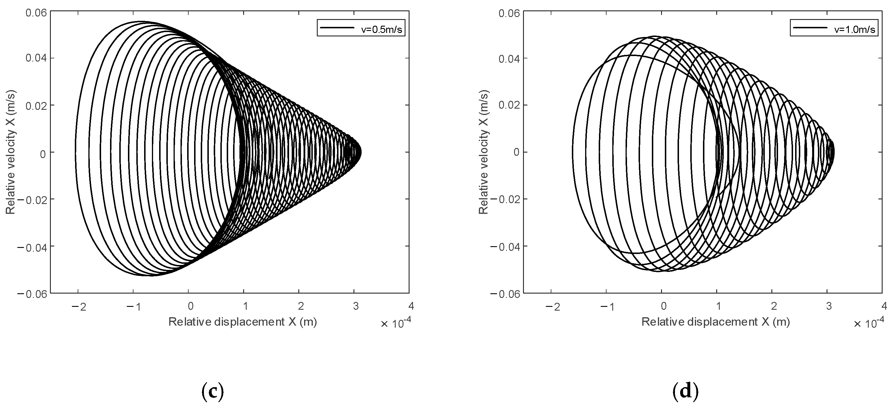
7.1.3. Effect of Driving Speed

This section analyzes the effect of different driving speeds on dynamic response and nonlinear characteristics of the mechanism, which are v = 0.5 m/s and v = 1.0 m/s with clearance joint B of 0.5 mm. The velocity and acceleration of block door, contact force of joint B, and driving force are analyzed.
As shown in Figure 14, the velocity, acceleration, contact force all increase with driving speed. Specifically, the maximum contact force almost tripled when the driving speed increases from 0.5 m/s to 1.0 m/s. When the blocker door starts to overturn, the driving force increases significantly with the increase of the driving speed. It can be seen in Figure 15 and Figure 16 that the increase in driving speed makes the distribution range of shaft center trajectory and phase diagram larger. Through Figure 17, it is found that the mapping points becomes more concentrated at higher driving speed, and the motion is more periodic. Compared with clearance joint A, the mapping points distribution is more dispersed at clearance joint B, which implies stronger nonlinearity there.

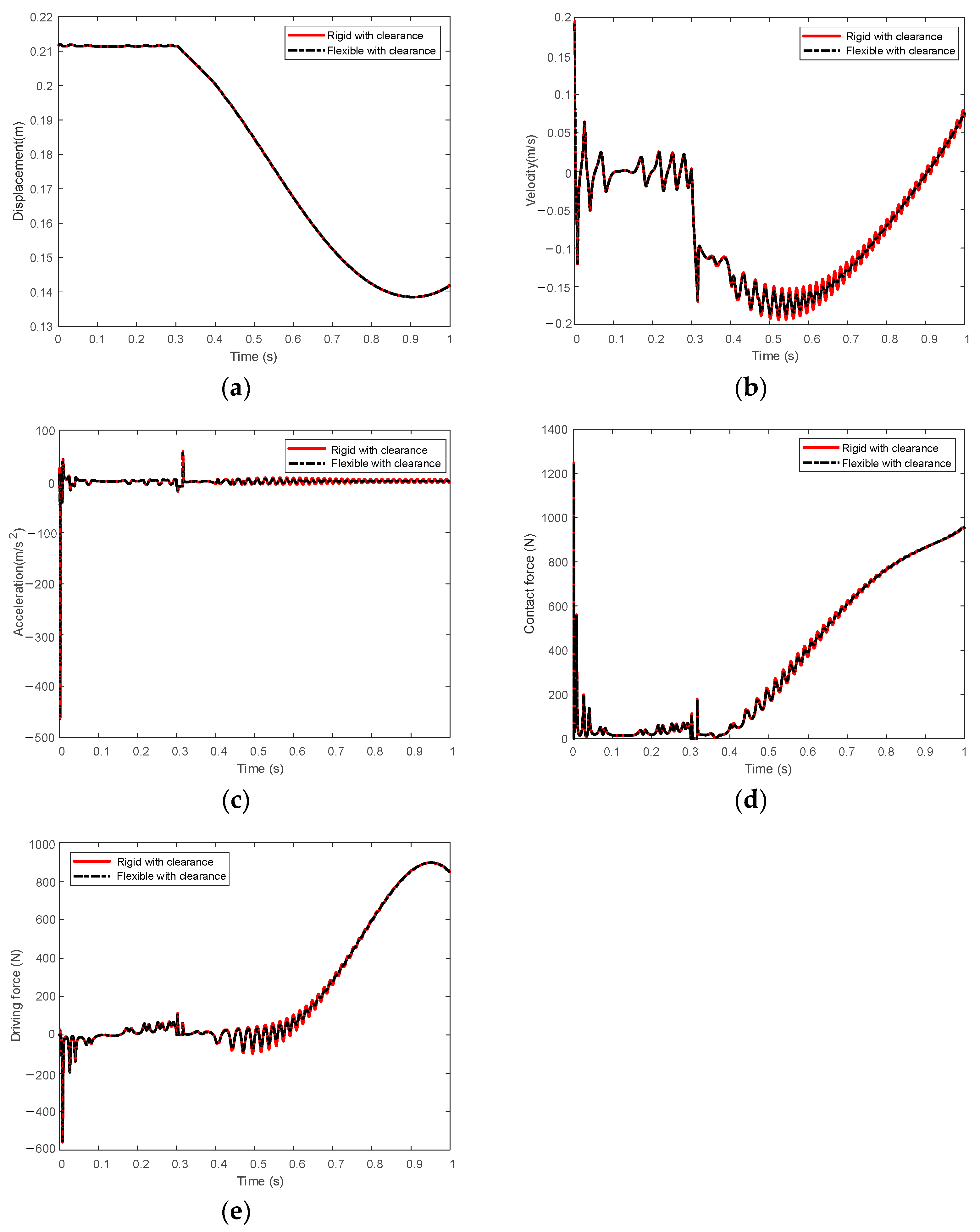
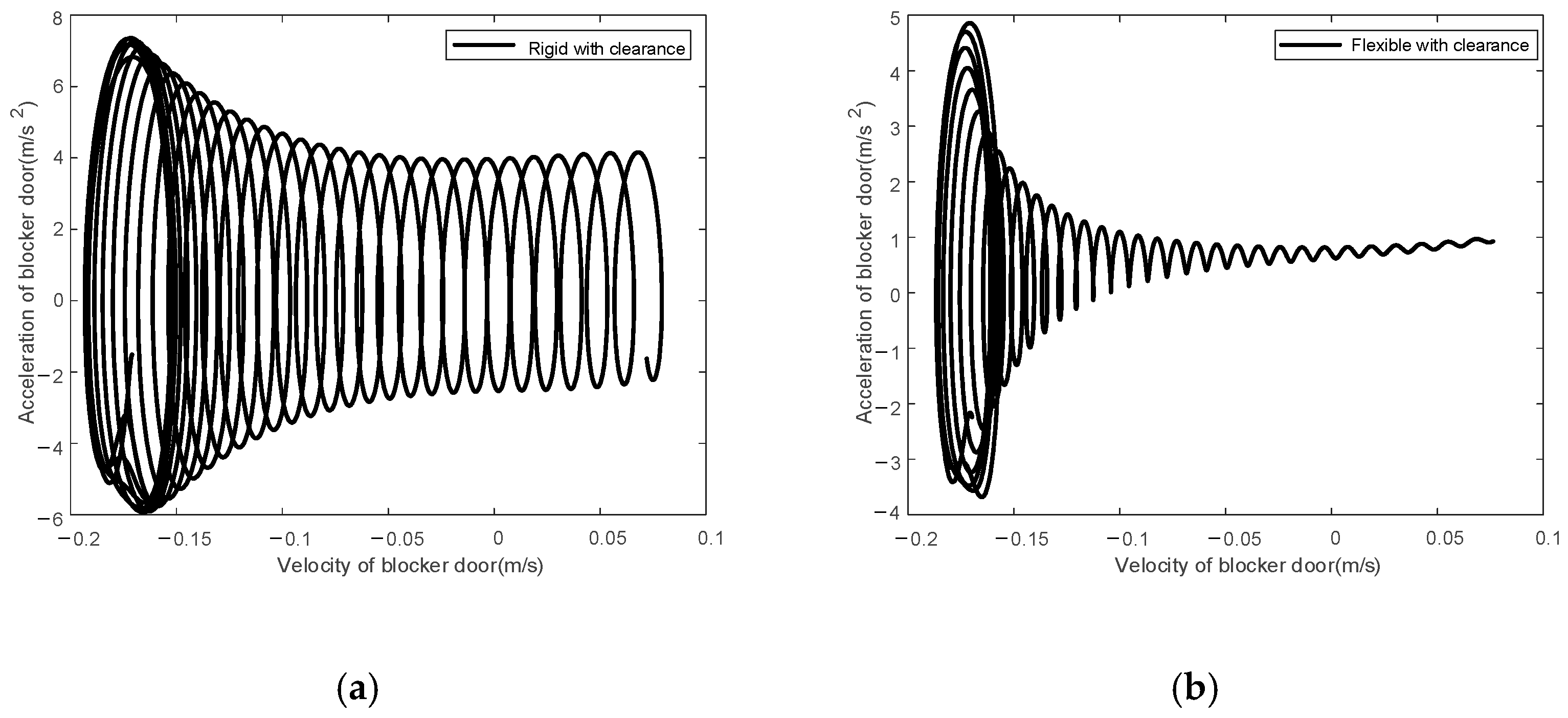
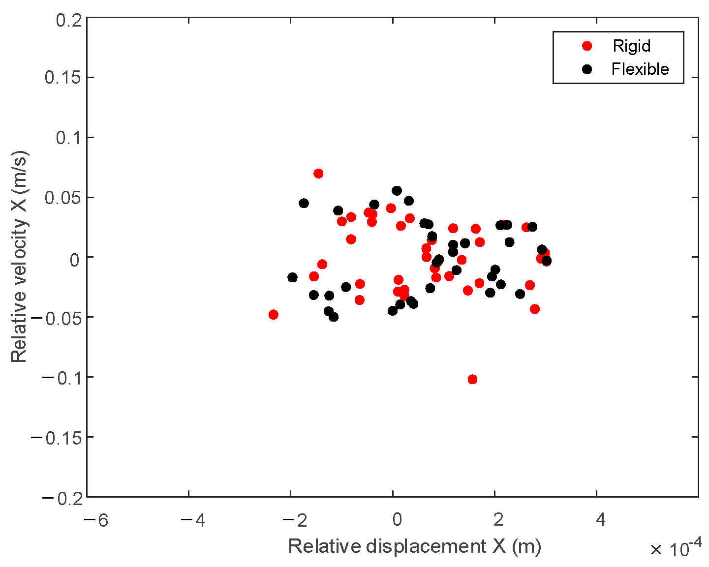
7.1.4. Effect of Flexible Component

The blocker rod is described as flexible, and the effect of the flexible component on the dynamic response of the mechanism is analyzed.
It can be found from Figure 18 that the displacements of blocker door with rigid rod and flexible rod basically coincide. The fluctuations of velocity, acceleration, contact force, and driving force are obviously weakened in the overturn stage with flexible rod. When the blocker door begins to overturn, the effect of the flexible rod becomes obvious with the increase of the load. The addition of the flexible body may introduce a damping effect for the system. It can be seen from Figure 19 that with flexible rod, the range of the shaft center trajectory is significantly reduced, which implies that the motion state at clearance is more stable. Through Figure 20, it is obvious that the range of phase diagram of blocker door with flexible rod is smaller than that of rigid mechanism, which implies that the relative acceleration is reduced, and the blocker door is more stable. As can be seen from Figure 21, the distribution of mapping points is more concentrated with flexible rod, so the flexible rod could weaken the nonlinear characteristics at the clearance and increase the stability of the motion of the mechanism.

7.2. Mechanism Simulation Parameters

The mobile fairing of the reverse thrust mechanism is simultaneously driven by three actuators, which are connected through a synchronous flexible shaft. When the actuators are asynchronous, the flexible shaft will generate synchronous torque and adjust the movement of the actuator. However, when the speed difference of the actuators is large enough, the adjustment of the flexible shaft would fail, causing the mechanism to be stuck, which would lead to serious accident.
Figure 22 shows the spatial multi-link reverse thrust mechanism, each mobile fairing is connected with five blocker doors, and three reverse thrust actuators arranged in the circumferential direction drive the mobile fairing and blocker door at the same time.
In order to study the influence of asynchronization of actuators on the mechanism blocking force, the reaction force of each actuator is observed at different conditions. It is assumed that under ideal synchronization conditions, the driving speed of the three actuators is 420 mm/s. In the case of asynchronous movement of the actuators, the speed of the three actuators is set to be 418 mm/s, 419 mm/s, 421 mm/s, and 422 mm/s respectively.
As shown in Figure 23, when the three actuators are driven synchronously, the actuators are mainly stressed in the X direction, and hardly in the Y and Z directions. Reaction forces of actuators 1 and 3 are basically the same, which is greater than that of actuator 2.
Since a major part of the reaction force of the actuator is in the X direction, in the subsequent sections only the X direction component of the reaction force is compared.
As can be seen from Figure 24, when the actuator 1 is asynchronous, the reaction forces of actuators 1 and 3 are basically similar and quite different from actuator 2, and the reaction force of the actuator 1 is greater than that of the actuator 3. The reaction forces of the actuators 1 and 3 increase with the decrease of driving speed of actuator 1, and the reaction force of the actuator 2 changes inversely. The maximum reaction force of the actuators 1, 2, and 3 are 2258 N, 1370 N, and 2017 N respectively.
When the actuator 2 is asynchronous, as can be seen from Figure 25, the reaction forces of actuators 1 and 3 are consistent, and opposite to the reaction force of actuator 2. When the driving speed increases, the reaction force on the actuator 1 and 3 increases and the reaction force on the actuator 2 decreases, which is opposite to the process of asynchronous drive of actuator 1. The maximum reaction force of the actuators 1, 2, and 3 are 2782 N, 2310 N, and 2712 N respectively.
Since the actuators 1 and 3 are symmetrically installed on the mobile fairing, when the actuator 3 is asynchronous, the reaction force of each actuator are consistent with asynchronous drive of actuator 1. As can be seen from Figure 26, the reaction force peaks of the actuators 1, 2, and 3 are 2068 N, 1348 N, and 2227 N respectively. It is found that the reaction force of each actuator is obviously larger when actuator 2 is driven asynchronously.

8. Conclusions

In this paper, the rigid flexible coupling dynamic model of cascade reverse thrust mechanism with clearance joint is established, and the effects of different factors on the dynamic response and nonlinear characteristics of the mechanism are studied. At the same time, through the spatial multi-link reverse thrust mechanism model, the influence of the asynchronous drive of actuators on the driving force of the mechanism is studied. The main conclusions of this study are as follows.
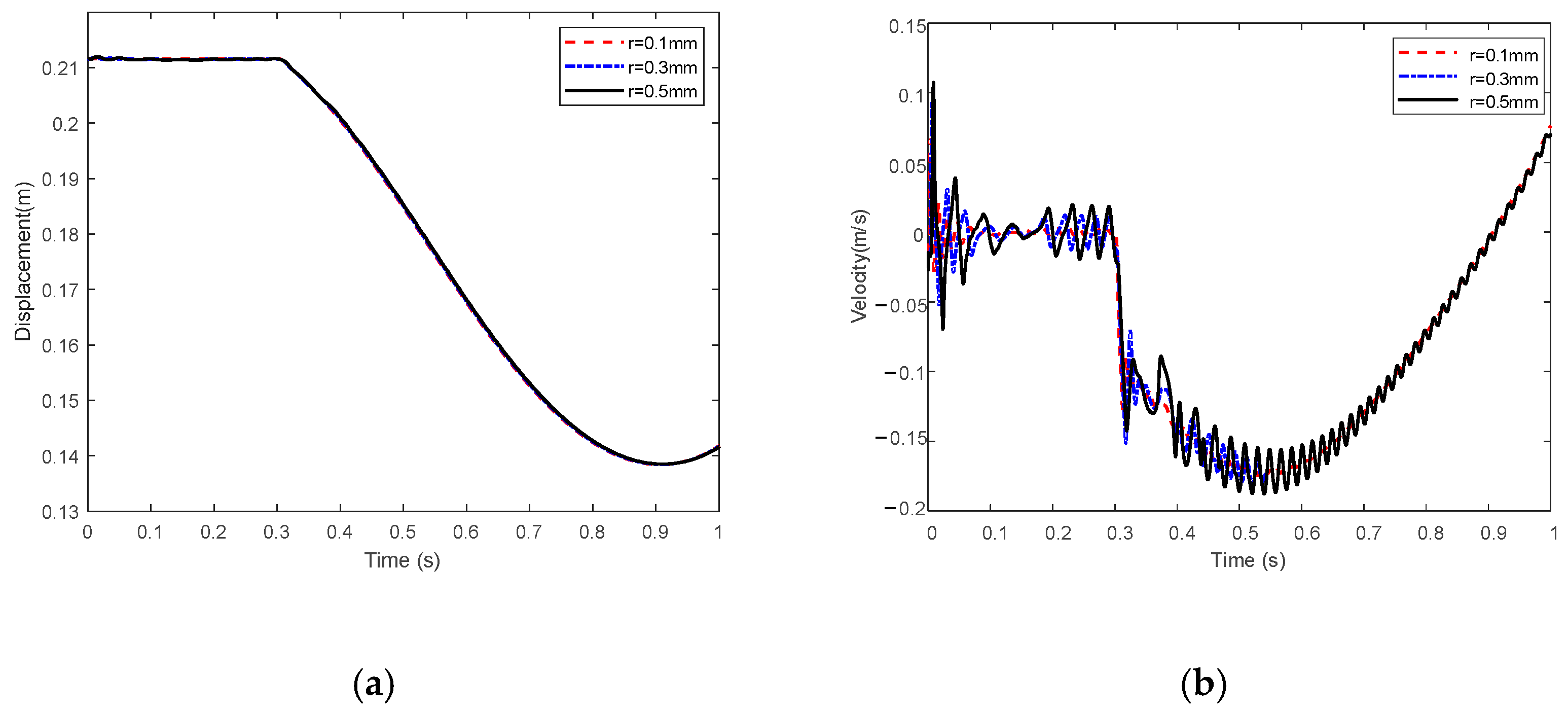
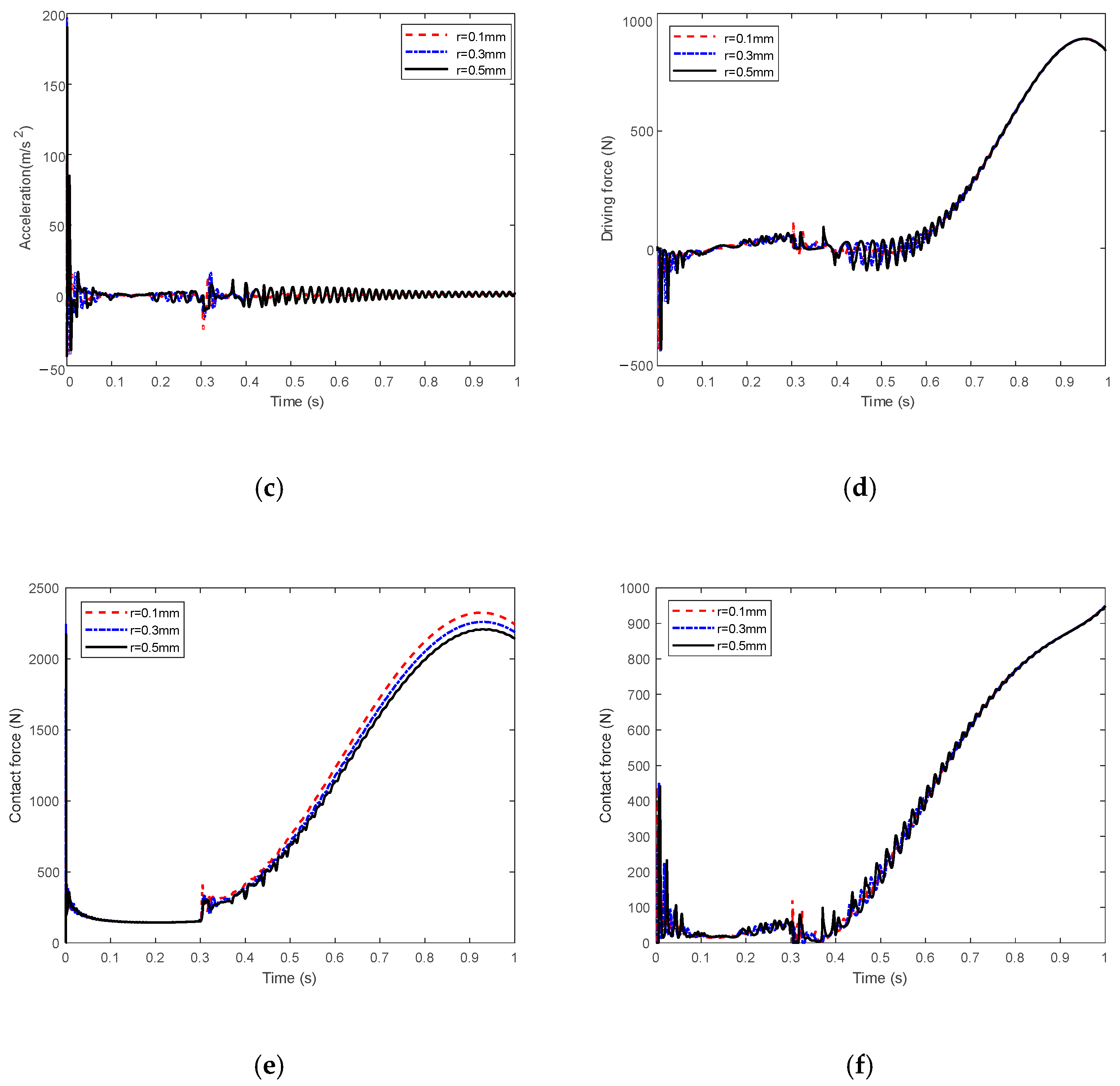
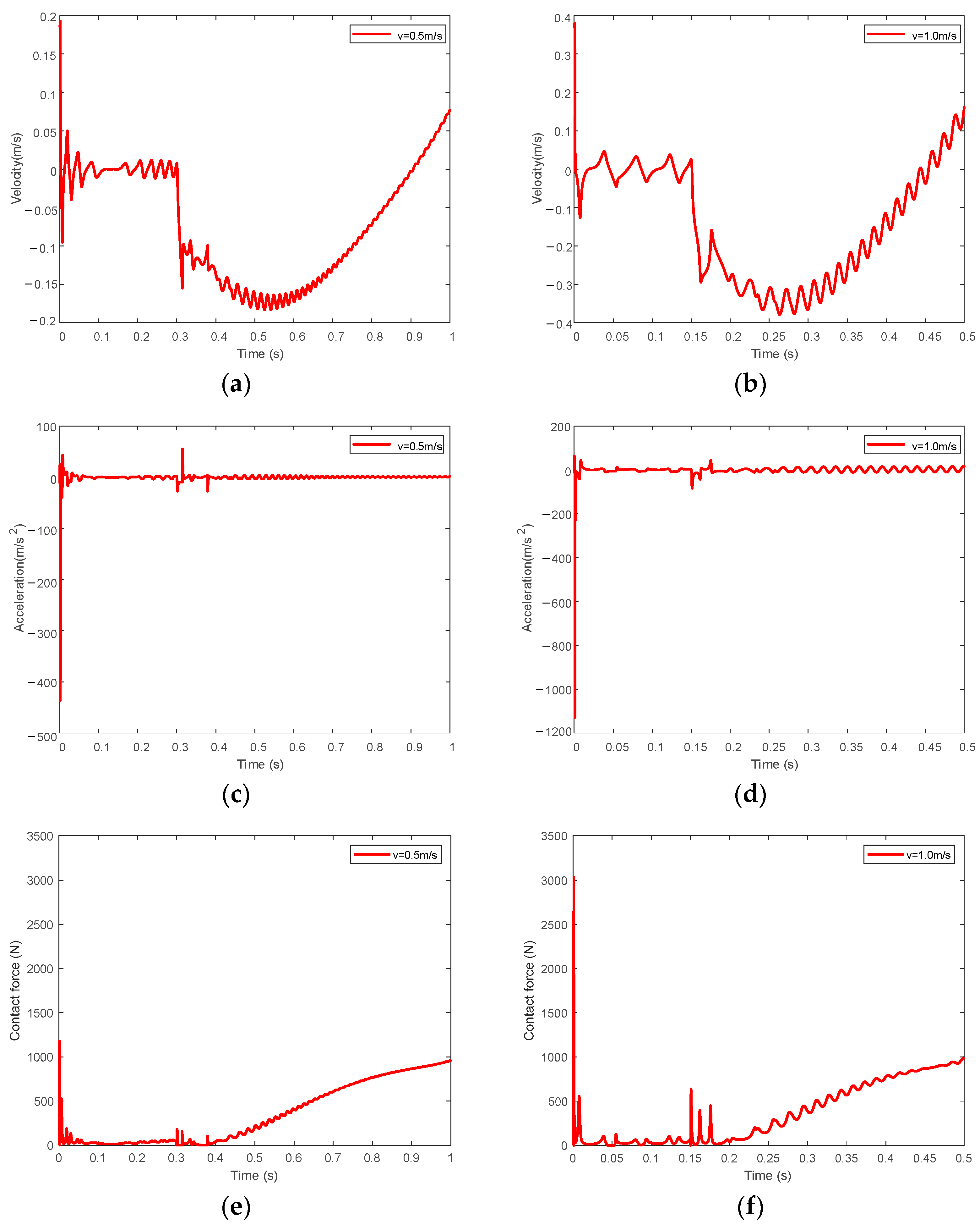
  • The influences of clearance value, clearance position, clearance value, flexible body, and driving speed on the dynamic response of the mechanism are analyzed. The results show that the vibration of the mechanism increases with the clearance value, the number of clearance joints, and the driving speed, while the addition of flexible parts can effectively weaken the vibration caused by the clearance and improve the stability of the mechanism.
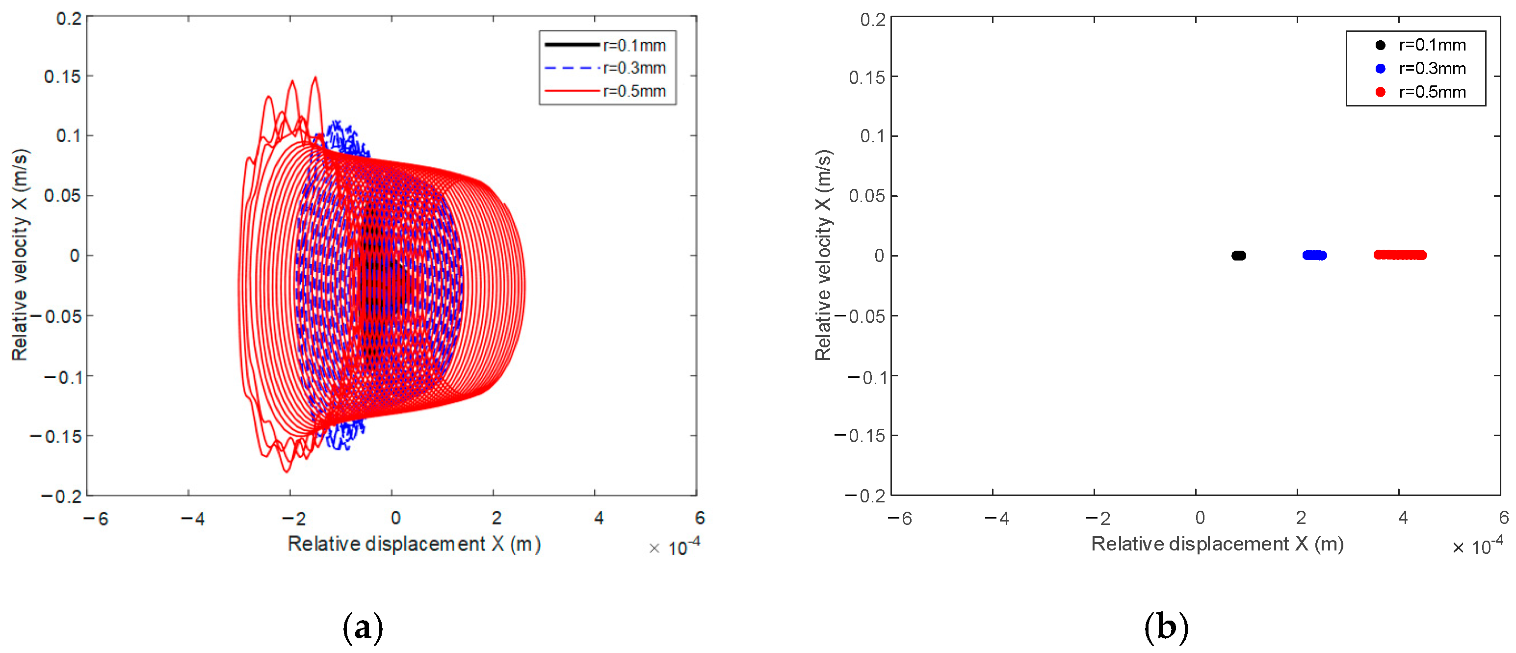
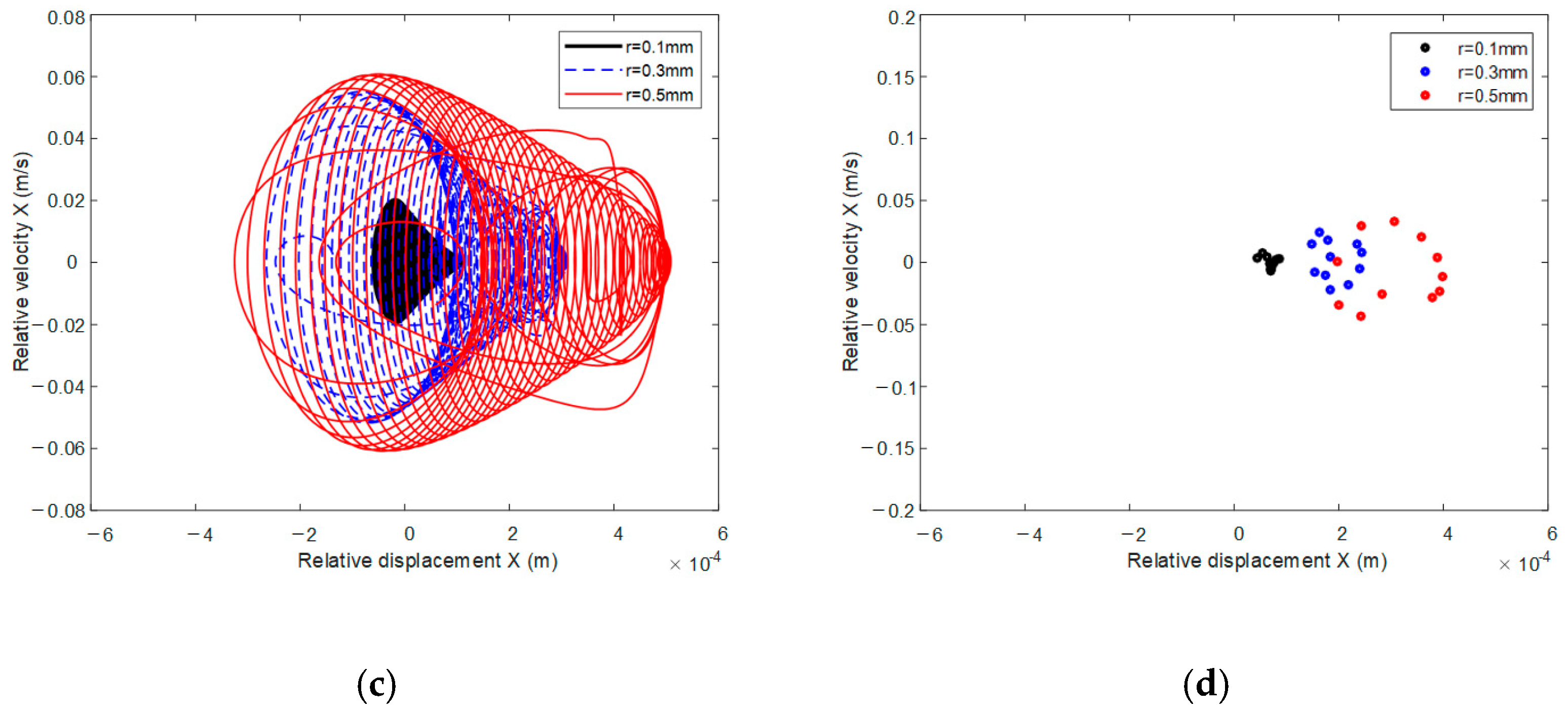
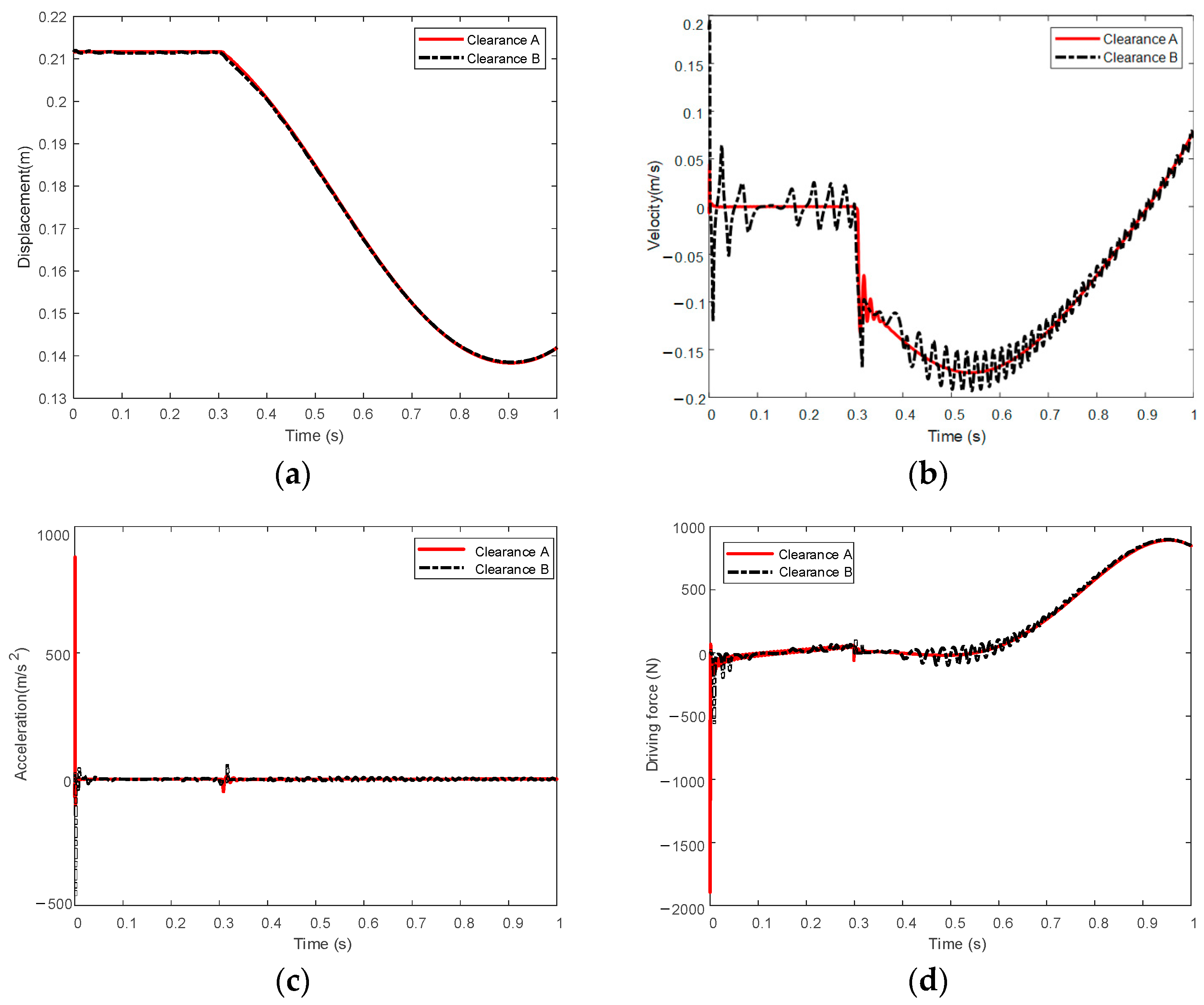
  • The phase diagram at the clearance show that the nonlinear characteristics of the mechanism increase with the clearance value, the number of clearance joints, and driving speed, while the flexible body can significantly improve the stability of the blocker door motion. At the same time, the influence of clearance joint B is more obvious than clearance joint A. Therefore, during the design and installation of the thrust reverse mechanism, the machining accuracy and installation accuracy of clearance B should be strictly controlled.
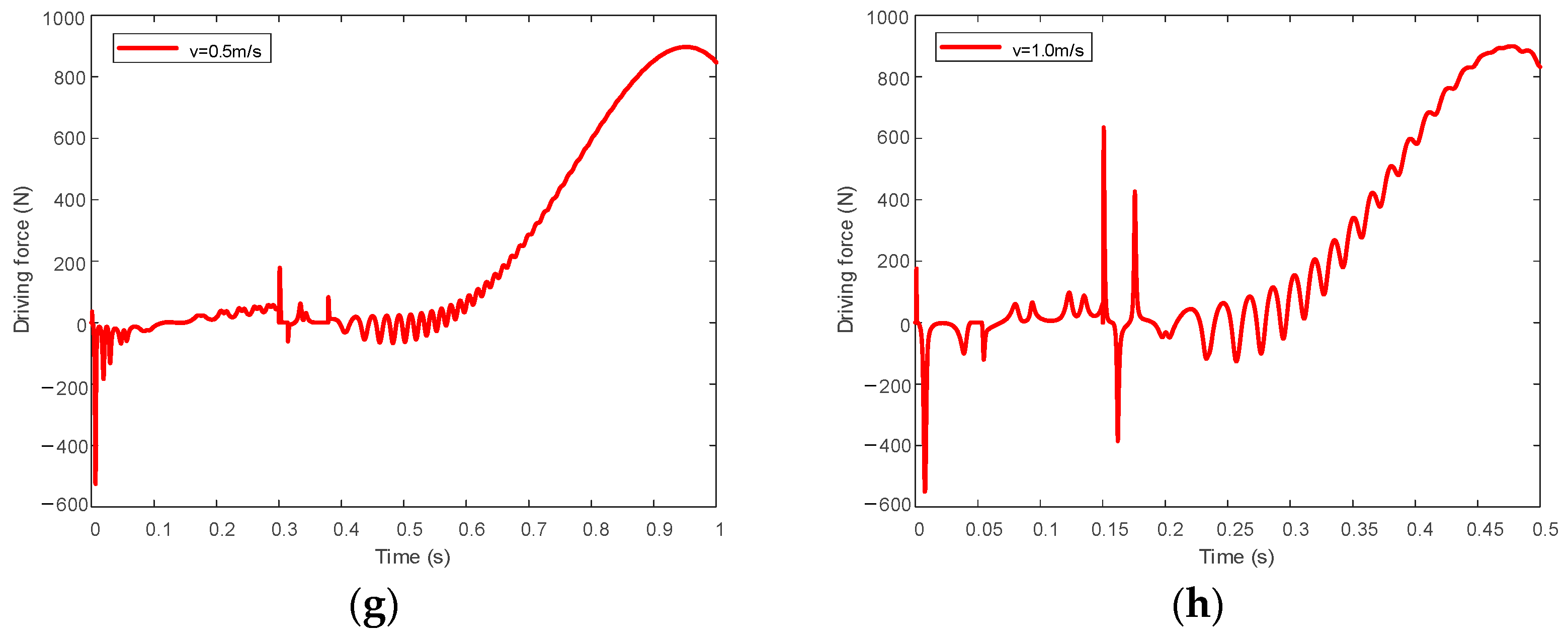
  • The reaction force of actuators 1 and 3 is consistent, and opposite to actuator 2. When the actuator 2 is asynchronous, the driving force of the mechanism is the largest. It can be seen from the change of driving force that when the asynchronous occurs, the driving speed of actuator 2 is lower than that of actuators 1 and 3, which can effectively reduce the peak driving force of actuators.

Author Contributions

Conceptualization, X.W. and J.Z.; methodology, X.W.; software, J.Z.; validation, X.W.; formal analysis, J.Z.; investigation, C.M.; resources, X.W. and C.M.; data curation, J.Z.; writing—original draft preparation, J.Z.; writing—review and editing, X.W.; visualization, J.Z.; supervision, Q.H.; project administration, Z.L.; funding acquisition, H.S. All authors have read and agreed to the published version of the manuscript.

Funding

This research was funded by the National Natural Science Foundation of China (52005088) and the Natural Science Foundation of Liaoning Province (2020-MS-076) and National Science and Technology Major Project (J2019-IV-0002-0069).

Informed Consent Statement

Not applicable.

Data Availability Statement

Not applicable.

Conflicts of Interest

The authors declare that they have no known competing financial interests or personal relationships that could have appeared to influence the work reported in this paper.

References

  1. Yetter, J.A. Why do airlines want and use thrust reverser? TM95-109158; NASA: Washington, DC, USA, 1995. [Google Scholar]
  2. Lei, W. Troubleshooting and maintenance of thrust reverser for 737NG aircraft. Civ. Aircr. Des. Res. 2018, 131, 85–90. [Google Scholar]
  3. Mahmood, T.; Jackson, A.; Rizvi, S.H.; Pilidis, P.; Savill, M.; Sethi, V. Thrust Reverser for a Mixed Exhaust High Bypass Ratio Turbofan Engine and its Effect on Aircraft and Engine Performance. Am. Soc. Mech. Eng. 2012, 17, 205–215. [Google Scholar]
  4. Liu, D. Intake and exhaust system Aeroengine Design Manual (Seventh Volume); Aviation Industry Press: Beijing, China, 2000. [Google Scholar]
  5. Yongqin, C.; Tianxing, W.; Sanmai, S.; Chao, L. Modeling and simulation of thrust reverser hydraulic actuation system based on AMESim. J. Aerosp. Power 2017, 32, 2791–2799. [Google Scholar]
  6. Mckay, B.; Barlow, A. The Ultra Fan Engine and Aircraft Based Thrust Reversing. In Proceedings of the AIAA/ASME/SAE/ASEE Joint Propulsion Conference & Exhibit, Atlanta, Georgia, 30 July–1 August 2012. [Google Scholar]
  7. Jin, B.; Xing, W.; Liu, D. Thrust reversers of aircraft/engine propulsion system. Aeroengine 2004, 30, 48–58. [Google Scholar]
  8. Du, G.; Jin, J. Large Transport aircraft engine reverse thrust device. In Proceedings of the Large Aircraft Key Technology High-level Forum and 2007 Annual Meeting of China Aviation Society, Shenzhen, China, 1–2 September 2008; pp. 375–385. [Google Scholar]
  9. Asbury, S.C.; Yetter, J.A. Static performance of six innovative thrust reverser concepts for subsonic transport applications. Summ. NASA Langley Innov. Thrust Reverser Test Program 2000. [Google Scholar]
  10. Zhang, G.; Wang, Q. The influence of main geometric parameters on the performance of cascade reverse thrust device. J. Aerosp. Power 2014, 27, 145–151. [Google Scholar]
  11. Wang, T. Research on Modeling and Simulation of Aircraft Thrust Reverse Device and Its Actuation System; Xidian University: Xi’an, China, 2017. [Google Scholar]
  12. Chen, Y.; He, J.; Su, S. Kinematics and dynamics simulation of thrust reverser. J. Aerosp. Power 2019, 34, 2316–2323. [Google Scholar]
  13. Zhang, S.; Wang, H.; He, J. Load and force transmission of cascade thrust reverser. J. Sichuan Ordnance 2015, 3, 56–59. [Google Scholar]
  14. Xie, Y.; Wang, Q.; Shao, W. Effect of kinetic mechanism of blocker doors on aerodynamic performance for a cascade thrust reverser. J. Aerosp. Power 2010, 25, 1297–1302. [Google Scholar]
  15. Chen, Z.; Shan, Y.; Shen, X. Numerica simulation of the Suction characteristics of thrust reverser when landing. J. Aerosp. Power 2016, 31, 733–739. [Google Scholar]
  16. Qiu, A.; Sang, W.; Xie, R. Numerical investigation on thrust reverse flow field of podded engines on blended wing body. J. Aerosp. Power 2021, 36, 1906–1916. [Google Scholar]
  17. Varsegov, V.L.; Shabalin, A.S. Selection of an optimal turbulence model for numerical flow simulation in a cascade type turbofan engine thrust reverser. Russ Aeronaut 2015, 58, 484–487. [Google Scholar] [CrossRef]
  18. Liu, C.; Deng, J.; Su, S. Design of Loading System for Thrust Reverser Ground Simulation Test. IOP Conf. Series Earth Environ. Sci. 2018, 170, 042093. [Google Scholar] [CrossRef]
  19. Shi, G.; Pan, J. Electro-hydraulic force servo system for simulating thrust in reverse of experimental systems on the ground for airplane. China Mech. Eng. 2010, 21, 42–45. [Google Scholar]
  20. Butterfield, J.; Yao, H.; Price, M.; Armstrong, C.; Raghunathan, S.; Benard, E.; Cooper, R.; Monaghan, D. Enhancement of thrust reverser cascade performance using aerodynamic and structural integration. Aeronaut. J. 2004, 108, 621–628. [Google Scholar] [CrossRef] [Green Version]
  21. He, J. Dynamic Analysis and Structure Optimizationof Aircraft Thrust Reverser; Xidian University: Xi’an, China, 2020. [Google Scholar]
  22. Roosenboom, E.W.M. Flow field Investigation at Propeller Thrust Reverse. J. Fluids Eng. 2010, 132, 0611011–0611018. [Google Scholar] [CrossRef]
  23. McCormick, R.L.; Koepcke, W.W.; Gallagher, J.T. Capabilities of in-flight thrust reversing. J. Aircr. 1969, 6, 263–268. [Google Scholar] [CrossRef]
  24. Cammarata, A.; Lacagnina, M.; Sinatra, R. Closed-form solutions for the inverse kinematics of the Agile Eye with constraint errors on the revolute joint axes. In Proceedings of the IEEE International Conference on Intelligent Robots and Systems, Daejeon, Korea, 9–14 October 2016; pp. 317–322. [Google Scholar]
  25. Lankarani, H.M.; Nikravesh, P.E. A Contact Force Model with Hysteresis Damping for Impact Analysis of Multibody Systems. J. Mech. Des. 1990, 112, 369–376. [Google Scholar] [CrossRef]
  26. Flores, P.; Koshy, C.S.; Lankarani, H.M.; Ambrósio, J.; Claro, J.C.P. Numerical and experimental investigation on multibody systems with revolute clearance joints. Nonlinear Dyn. 2011, 65, 383–398. [Google Scholar] [CrossRef] [Green Version]
  27. Erkaya, S. Experimental investigation of flexible connection and clearance joint effects on the vibration responses of mechanisms. Mech. Mach. Theory 2018, 121, 515–529. [Google Scholar] [CrossRef]
  28. Flores, P.; Lankarani, H.M. Dynamic response of multibody systems with multiple clearance joints. J. Comput. Nonlinear Dyn. 2012, 7, 031003. [Google Scholar] [CrossRef]
  29. Machado, M.; Moreira, P.; Flores, P.; Lankarani, H.M. Compliant contact force models in multibody dynamics: Evolution of the Hertz contact theory. Mech. Mach. Theory 2012, 53, 99–121. [Google Scholar] [CrossRef]
  30. Den Hartog, J.P. Forced vibrations with combined coulomb and viscous friction. Trans. ASME 1993, 19, 107–115. [Google Scholar]
  31. Ambrósio, J.A.C. Impact of rigid and flexible multibody systems: Deformation description and contact models. In Virtual Non-Linear Multibody Systems; Springer: Dordrecht, The Netherland, 2003; pp. 57–81. [Google Scholar]
  32. Shabana, A.A. An Absolute Nodal Coordinates Formulation for the Large Rotation and Deformation Analysis of Flexible Bodies; Technical Report. No. MBS96-1-UIC; University of Illinois at Chicago: Chicago, IL, USA, 1996. [Google Scholar]
  33. Shabana, A.A. Computer Implementation of the Absolute Nodal Coordinate Formulation for Flexible Multibody Dynamics. Nonlinear Dyn. 1998, 16, 293–306. [Google Scholar] [CrossRef]
  34. Gerstmayr, J.; Shabana, A.A. Analysis of Thin Beams and Cables Using the Absolute Nodal Coordinate Formulation. Non-Linear Dyn. 2006, 45, 109–130. [Google Scholar] [CrossRef]
Figure 1. Mechanism of cascade thrust reverser system. 1. fixed support; 2. large pull rod; 3. transfer pull rod; 4. mobile fairing; 5. cascade; 6. torsion spring; 7. limit lug; 8. blocker door.
Aerospace 09 00611 g001
Figure 2. Clearance joint model. (a) “Free flight” mode. (b) “Contact deformation” mode.
Aerospace 09 00611 g002
Figure 3. Friction model. (a) Coulomb friction model. (b) Modified coulomb friction model.
Aerospace 09 00611 g003
Figure 4. Flexible beam element model.
Aerospace 09 00611 g004
Figure 5. Flowchart of solving rigid-flexible coupling dynamic equation.
Aerospace 09 00611 g005
Figure 6. Flexible pendulum model in three dimensional motion.
Aerospace 09 00611 g006
Figure 7. Comparison between simulation results and the results of former literature. (a) The Z versus X position of the tip of the pendulum. (b) The Y position of the mid-point of the pendulum.
Aerospace 09 00611 g007
Figure 8. Aerodynamic load on the blocker door.
Aerospace 09 00611 g008
Figure 9. Kinematics of blocker door and contact force at clearance joint with different clearance values (a) Displacement of blocker door. (b) Velocity of blocker door. (c) Acceleration of blocker door. (d) Driving force. (e) Contact force at clearance A. (f) Contact force at clearance B.
Aerospace 09 00611 g009aAerospace 09 00611 g009b
Figure 10. Phase diagram and Poincare map at clearance joints. (a) Phase diagram at clearance joint A. (b) Poincare map at clearance joint A. (c) Phase diagram at clearance joint B. (d) Poincare map at clearance joint B.
Aerospace 09 00611 g010aAerospace 09 00611 g010b
Figure 11. Comparison of kinematics of blocker door and the driving force with clearance joint at different positions. (a) Displacement of blocker door. (b) Velocity of blocker door. (c) Acceleration of blocker door. (d) Driving force of mechanism.
Aerospace 09 00611 g011
Figure 12. Shaft center trajectory and phase diagram at clearance. (a) Shaft center trajectory at clearance joint A. (b) Phase diagram at clearance joint A. (c) Shaft center trajectory at clearance joint B. (d) Phase diagram at clearance joint B.
Aerospace 09 00611 g012aAerospace 09 00611 g012b
Figure 13. Phase diagram of blocker door. (a) Clearance joint A = 0.3 mm. (b) Clearance joint B = 0.3 mm.
Aerospace 09 00611 g013
Figure 14. Comparison of the kinematics of blocker door, contact force and driving force with driving speed. (a) Velocity of blocker door at 0.5 m/s. (b) Velocity of blocker door at 1.0 m/s. (c) Acceleration of blocker door at 0.5 m/s. (d) Acceleration of blocker door at 1.0 m/s. (e) Contact force at 0.5 m/s. (f) Contact force at 1.0 m/s. (g) Driving force at 0.5 m/s. (h) Driving force at 1.0 m/s.
Aerospace 09 00611 g014aAerospace 09 00611 g014b
Figure 15. Shaft center trajectory at clearance joints A and B. (a) Clearance joint A. (b) Clearance joint B.
Aerospace 09 00611 g015
Figure 16. Phase diagram at clearance joint A and clearance joint B. (a) Clearance joint A, v = 0.5 m/s. (b) Clearance joint A, v = 1.0 m/s. (c) Clearance joint B, v = 0.5 m/s. (d) Clearance joint B, v = 1.0 m/s.
Aerospace 09 00611 g016aAerospace 09 00611 g016b
Figure 17. Poincare map at clearance joints A and B. (a) Clearance joint A. (b) Clearance joint B.
Aerospace 09 00611 g017
Figure 18. Comparison of the kinematics of blocker door, contact force and driving force between flexible and rigid pull rod with clearance joint. (a) Displacement of blocker door. (b) Velocity of blocker door. (c) Acceleration of blocker door. (d) Contact force at clearance B. (e) Driving force of mechanism.
Aerospace 09 00611 g018
Figure 19. Shaft center trajectory at clearance joint B. (a) Rigid with clearance. (b) Flexible with clearance.
Aerospace 09 00611 g019
Figure 20. Phase diagram at blocker door. (a) Rigid with clearance. (b) Flexible with clearance.
Aerospace 09 00611 g020
Figure 21. Poincare map of rigid and flexible.
Aerospace 09 00611 g021
Figure 22. Spatial multi-link mechanism of cascade thrust reverse system.
Aerospace 09 00611 g022
Figure 23. Reaction force of actuators when the three actuators are driven synchronously. (a) Reaction force in X direction. (b) Reaction force in Y direction. (c) Reaction force in Z direction.
Aerospace 09 00611 g023
Figure 24. Reaction force of actuators when the actuator 1 is asynchronously driven. (a) Actuator1 in X direction. (b) Actuator2 in X direction. (c) Actuator3 in X direction.
Aerospace 09 00611 g024
Figure 25. Reaction force of actuators when the actuator 2 is asynchronously driven. (a) Actuator1 in X direction. (b) Actuator2 in X direction. (c) Actuator3 in X direction.
Aerospace 09 00611 g025
Figure 26. Reaction force of actuators when the actuator 3 is asynchronously driven. (a) Actuator1 in X direction. (b) Actuator2 in X direction. (c) Actuator3 in X direction.
Aerospace 09 00611 g026
Table 1. Structural parameters.
ParameterValue
Model length1.0 m
Element density3.20 × 102 kg/m3
Young’s modulus1.60 × 106 N/m2
Poisson’s ratio 0
Cross section area2.50 × 10−5 m2
Initial angular velocity4.0 rad/s
Integration step size0.001 s
Table 2. Structural parameters.
ComponentLength (m)Mass (kg)Moment of Inertia (m4)
large pull rod0.220.52.01 × 10−7
transfer pull rod0.0360.21.94 × 10−9
blocker door0.1955.07.49 × 10−6
mobile fairing0.8050.02.46 × 10−5
limit lug0.0550.18.30 × 10−10
Table 3. Parameters of clearance.
ParameterValue
Bearing radius0.01 m
Bearing width0.015 m
Young’s modulus207 Gpa
Poisson’s ratio 0.29
Friction coefficient0.3
Restitution coefficient0.9
Tangential velocity V10.001 m/s
Tangential velocity V00.0001 m/s
Integration step size0.001 s
Table 4. Parameters of flexible component.
ParameterValueParameterValue
Young’s Modulus (Gpa)207Sectional area A (m2)0.002
Density (kg/m3)7850Section moment of inertia If (m4)2.01 × 10⁻⁷
Publisher’s Note: MDPI stays neutral with regard to jurisdictional claims in published maps and institutional affiliations.

