Prediction of Crack Growth Life at Elevated Temperatures with Neural Network-Based Learning Schemes

Abstract

Applying the machine learning (ML) technique in the modelling of crack growth (CG) behavior is a potential way to improve the efficiency and precision of CG assessment. However, research in this field at elevated temperatures is limited, although a lot of achievements have been obtained in CG assessment at room temperature. Neutral network (NN)-based methods to model the CG at elevated temperatures were therefore investigated in this paper. An “indirect” method (NNK method) assessing the CG by modelling and integrating the crack growth rate (CGR) was established. A “direct” method (ENNIL method) was built by further developing the NN-based increment learning scheme. The NNK method shows high accuracy in CG prediction with relatively short CG life, while the ENNIL method gives perfectly predicted results for cases with relatively long CG life. The combination of these two methods may be an effective way to further improve CG assessment at elevated temperatures.

1. Introduction

Key structural components in a series of important equipment, such as aircraft engine, pressure vessel and power generation et al., serve in elevated temperature environments. Crack growth (CG) assessment needs to be carried out on some of these components (turbine disk et al.) in order to ensure structure integrity. However, the accuracy of CG assessment is always limited. This is because of the difficulty in the quantitative description of CG with the significant effect of temperature and the existence of creep-fatigue (CF) coupling effects [1,2]. Many investigations have therefore been carried out on modelling CG behavior at elevated temperatures, especially under CF interactive conditions [3,4].

Most of these investigations are focused on developing the crack growth rate (CGR) model (the formula between crack driving force (CDF) and CGR), because the CG curves (a-N curves) can be predicted via integration of CGR. Tong and Onofrio et al. [5,6] established earlier CGR models at elevated temperatures by modifying the material constants (C, n) in the Paris law (da/dN_fatigue = C(ΔK)ⁿ [7]). Djavanroodi and Whittaker et al. [8,9] considered the existence of both fatigue effects and creep effects in the failure at elevated temperatures. They thought the effects of fatigue and creep to be independent and presented a group of CF linear superposition models (da/dN = (da/dN)_fatigue + (da/dN)_creep). Grover, Shlyannikov and Yang et al. [10,11,12] further developed CF superposition models by adding a term to consider the CF interactive effects, such as da/dN = (da/dN)_fatigue + (da/dN)_creep + (da/dN)_interaction. Their CGR models further improve calculation accuracy. However, no one of above mentioned CGR models was widely accepted in CG analysis, untill now. The reason is that these CGR models fail to generalize to a wide temperature and loads range, in the prediction of CG curves, as they depend on human knowledge to a large extent.

Some methods modelling the CG at elevated temperatures were established based on the numerical simulation technique. In most of these investigations, the crack tip field was simulated by building the Finite Element (FE) model with visco-plastic constitutive and then the CG was modelled based on the simulated crack tip field. Lepore [13] calculated the evolution of crack driving force based on the simulated crack tip field and modelled the CGR based on the CGR model. Lianyong [14] calculated the accumulated damage under the interacted effects of CF, utilizing the non-linear summation approach. After the accumulated damage of the element reached a critical value, nodes were released to model the CGR. In other research [15,16], an irreversible cohesive zone model was applied in the FE model to describe material damage during crack propagation. The above numerical simulation-based methods usually achieved good agreement with experimental data. However, they require the complex constitutive model to describe material properties under the CF condition and high calculation costs to simulate step-by-step the CG, thus retarding the wide application of NS-based methods into the engineering field.

The application of the machine learning (ML) technique in the CG modelling at elevated temperatures (ML-based method) seems to be the potential way to solve the above issues. Although limited ML research of CGR at elevated temperatures can be found, the research of applying ML-based methods in the fatigue and FCG analysis at room temperature (which show great learning and generalization ability) has indicated this. Morse [17] used the dual boundary element method to model fatigue crack growth and used the machine learning to decrease the calculation costs successfully. Enrico [18] and Hu [19] developed the Bayesian-based calibration method and achieved greater accuracy, higher computational efficiency and better uncertainties analysis in the fatigue crack growth (FCG) life prediction of complex components, such as turbine discs. Mortazavi [20] established a radial basis function artificial neural network model, which shows good interpolation capability in the prediction of both short and long FCG behavior in Ti-6Al-4V, 2024-T3 and 7075-T6 alloys.

The neutral network (NN) is a typical ML technique. It has been applied to model the CGR and shows advantages in FCG prediction at room temperature. Mohanty [21] trained a nine-layer NN to simulate the CGR of aluminum alloys by learning CGR data with six stress ratios (R = 0, 0.2, 0.4, 0.6, 0.7, 0.8) and used this NN to predict the CGR under R = 0.5. Zhang [22] trained a radial basis function artificial NN to calculate the CGR for different aluminum alloys. Both Mohanty and Zhang achieved good agreement with CGR experimental data, but the calculated a-N curves used the integration method based on their predicted CGR data deviated from experimental data. Due to the existence of significant deviation in the prediction of a-N curves using the integration method, some researchers directly predicted a-N curves using the NN based methods. Palakal [23] predicted the evolution of crack length under various arbitrary aircraft spectrum loadings using back-propagation NN. Do [24] utilized long short-term memory and multi-layer NN to successfully forecast the next propagation of a crack. Xiaofan [25] developed an NN-based increment learning scheme for the prediction of a-N curves. The trained network via this scheme can give satisfactory results with a significantly small amount of data, thus providing a new direction for the further development of NN-based methods in the CG prediction.

Although NN-based methods have shown significant advantages in CG prediction at room temperature, they were not widely applied in the CG prediction at elevated temperature until now. In terms of this issue, the NN-based methods performing well at room temperature were extended to CG prediction at elevated temperatures in this paper. The “indirect” NN-based method assessing the CG at elevated temperature by modelling and integrating the CGR was investigated. The “direct” NN-based methods building the relationship between a and N by using NN was developed based on the NN-based increment learning scheme. These methods not only extend the generalization of the previous NN-based method, but also provide high accuracy predicted results with low calculation costs, thus promoting the further improvement of CG prediction at elevated temperatures.

2. Materials and Methods

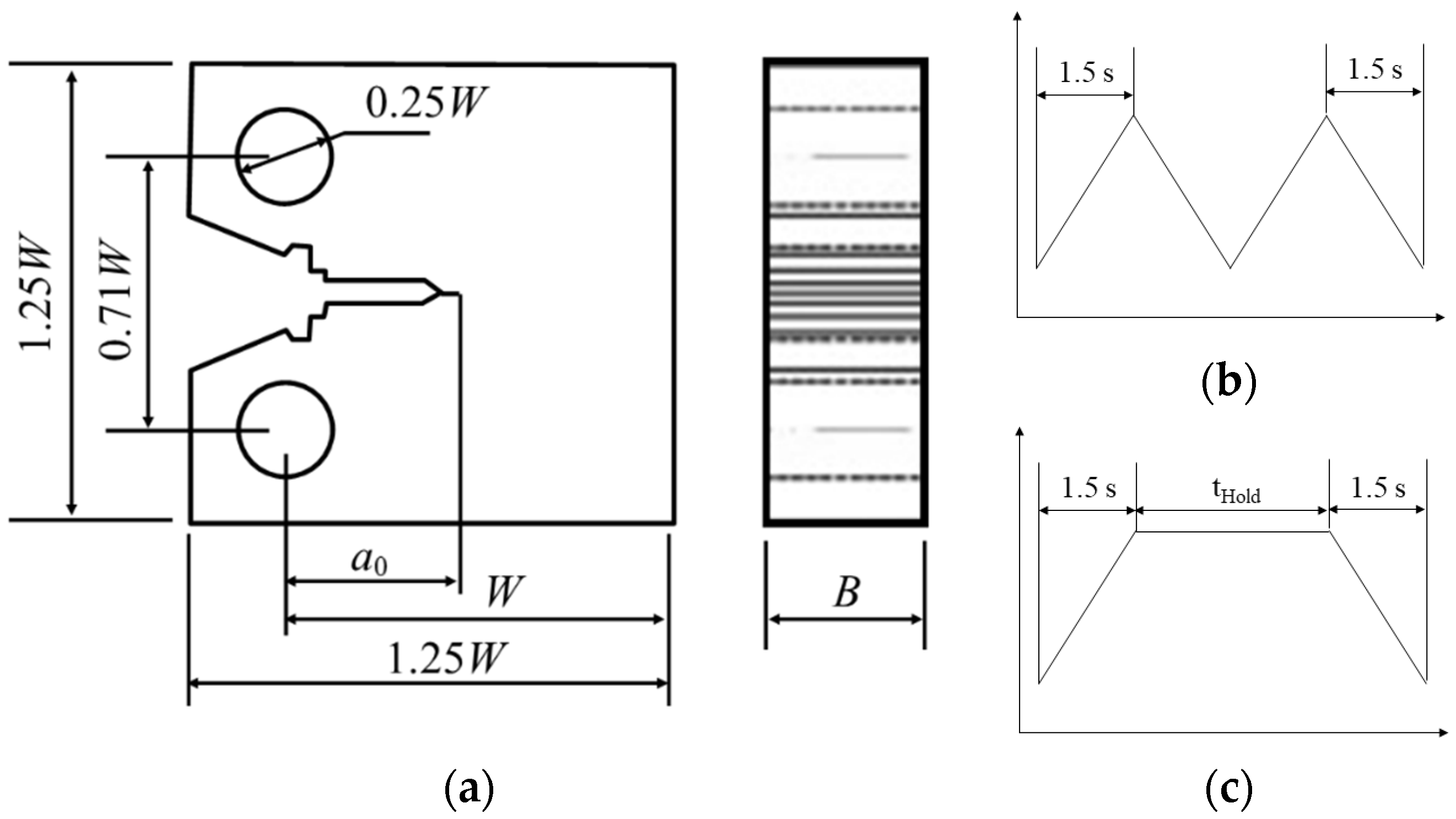
2.1. Experimental CG Data of FGH97 at Elevated Temperatures

CG data previously presented by our research group [26,27,28] are served as the input data for the NN learning in this research. These data were measured by carrying out CG tests on compact tension specimens with 50 mm width and 25 mm thickness (see Figure 1a). Specimens were manufactured by a nickel-based superalloy FGH97, whose nominal chemical composition is listed in

Table 1. Nominal chemical composition of FGH97 (wt.%) [27].

C	Cr	Mo	W	Al	Ti	Co	Nb	Hf	Mg	Zr	B	Ce	Ni
0.02–0.06	8.0–10	3.5–4.2	5.2–5.9	4.8–5.3	1.6–2.0	15.0–16.5	2.4–2.8	0.1–0.4	≤0.02	≤0.02	≤0.02	≤0.01	Remains

. The average grain size and the amount of γ’ precipitates for this material are about 30 μm and 62.4 wt.%, respectively [29]. Loading waveforms used in CG tests were triangular wave and trapezoidal wave (schematically shown in Figure 1b,c). Figure 1b is the 1.5 s–1.5 s triangular wave used to measure the FCG data. Figure 1c is the trapezoidal wave formed by superimposing different dwell time at the peak load to the triangular wave, which is used to measure CG data under CF conditions (CFCG data).

CG data under 16 service conditions (listed in

Table 2. Groups of CG data under various loading conditions at elevated temperatures.

Dataset Name	Condition Name	T (°C)	tHold (s)	PMax (kN)	PMin (kN)	Type
Data 1	C1	550	0	18	0.9	F
Data 2	C2	650	0	18	0.9	F
Data 3	C3	650	90	18	0.9	CF
Data 4	C4	650	90	20	1	CF
Data 5	C5	650	90	33	1.65	CF
Data 6	C6	670	90	30	1.5	CF
Data 7	C7	690	90	24.5	1.2025	CF
Data 8	C8	710	90	20	1	CF
Data 9	C9	750	0	18	0.9	F
Data 10	C10	750	1500	16	0.8	CF
Data 11	C11	750	1500	20	1	CF
Data 12	C12	750	25	18	0.9	CF
Data 13	C13	750	450	18	0.9	CF
Data 14	C14	750	90	14	0.7	CF
Data 15	C15	750	90	18	0.9	CF
Data 16	C16	750	90	20	1	CF

) with the same load ratio (R = P_Min/P_Max = 0.05) were used in this research as the basic dataset of machine learning. These conditions cover 550–750 °C temperature (T), 0–1500 s holding time (t_Hold), 14–33 kN maximum load (P_Max) and 0.9–1.65 kN minimum load (P_Min), reflecting the interactive effect of temperature, holding time and load level on the CG. For these 16 conditions, only CGR data (da/dN-ΔK) were presented previously but the raw data (a-N) of CG tests were not reported. In order to fulfil the requirement of ML in this research, the a-N data for these 16 conditions are published in this paper. It should be noted that all data for the 16 conditions (over 600 data points in total) are not shown in this section. They are shown in Section 3, together with the ML predicted results.

2.2. NN-Based Methods for CG Prediction

The back propagation neutral network (BPNN) is a NN successfully used in CG prediction at room temperature. It consists of an input layer, one or more hidden layers and an output layer. In this research, BPNN with one hidden layer was used to model the CG at elevated temperature. Four groups of methods based on different BPNN (BPNN with different input and output parameters) were investigated. Their detailed information is listed in

Table 3. List of NN-based methods for predicting CG at elevated temperatures.

Method	NN Name	NN Input	NN Output
NNK	NNK-K	Kmax, ΔK	da/dN
	NNK-KT	Kmax, ΔK, T
	NNK-KTt	Kmax, ΔK, T, tHold
RNN	RNN-N	N	a
NNIL	NNIL-N	N, ΔN′	a, Δa′
ENNIL	ENNIL-a	a, ΔN	Δa
	ENNIL-aP	a, ΔN, PMax, PMin
	ENNIL-aPT	a, ΔN, PMax, PMin, T
	ENNIL-aPTt	a, ΔN, PMax, PMin, T, tHold

.

NNK is the only one “indirect” NN-based method in these methods. The “indirect” means that the NN in this method is used to model the CGR rather than the CG (a-N curves). The CG prediction is indirectly achieved by integrating the modelled CGR in the NNK method, see Figure 2. In the NN of this method, the maximum intensity factor (K_max) and the range of intensity factor (ΔK) were selected as input parameters because they were usually used in the formula of CF CGR models to represent the effect of CDF. Their values were calculated based on ASTM standard [30] using following equations:

$$\Delta K=\frac{\Delta P}{B\sqrt{W}}·\frac{\left(2+\alpha \right)}{{\left(1-\alpha \right)}^{3/2}}\left(0.886+4.64\alpha -13.32{\alpha }^2+14.72{\alpha }^3-5.6{\alpha }^4\right)$$

(1)

$$K_{max}=\Delta K/\left(1-R\right)$$

(2)

where B and W are sample dimensions marked in Figure 1a; R is the stress ratio; α is equal to a/W; ΔP is equal to P_max − P_min.

Temperature (T) and duration of dwelling time (t_Hold) were also served as input parameters of NN to consider the effect of elevated temperature and the related CF interactive effect. It should be noted that three types of NN (see NNK-K, NNK-KT and NNK-KTt in Table 3) were investigated in the research of NNK method. The design of them is to describe a group of CG under various conditions, such as the CG under interactive effect of K_max, ΔK, T and t_Hold (NNK-KTt), CG under the constant t_Hold (NNK-KT) and CG under the constant T and t_Hold (NNK-K).

The RNN, NNIL and ENNIL methods listed in Table 3 are “direct” NN-based methods, which use NN to model the CG (a-N curves) directly. The RNN method adopts the simplest type of NN to directly build the relationship between number of cycles (N) and crack length (a). Its network structure consists of an input layer with one neuron (N), one hidden layer with multiple neurons and an output layer with one neuron (a).

The NNIL method is the NN-based increment learning scheme. Two types of NNIL methods were investigated in this research. They are NNIL-N and NNIL-NP listed in Table 3. NNIL-N is Xiaofan’s NN-based increment learning scheme [25]. The information for NNIL-N is shown in Figure 3. Figure 3a presents the NN structure: inputs are N and its increment (ΔN′); the number of hidden layers is one; outputs are a and its increment (Δa′). Figure 3b demonstrates the way to generate training dataset (a, Δa′, N, ΔN′) for NN, where a and N are experimental measured values. Δa′ and ΔN′ are difference values between a pair of experimental points.

In this way, an experimental dataset (a, N) with the size of n can generate a training dataset (a, Δa′, N, ΔN′) with the size of n × (n − 1)/2. This means a significant increase of input information for the training of NN. In this way, this method gets over the shortage of using BPNN to model the CG (not good at training on small dataset).

The ENNIL method is a NN-based method developed in this research. It is established by improving the NNIL method via fully considering the effect of more input parameters. Three types of NN listed in Table 3 were used in the ENNIL method to model CG under different conditions, such as the CG under interactive effect of P_max, P_min, T and t_Hold (ENNIL-aPTt), CG under the constant t_Hold (ENNIL-aPT) and CG under the constant T and t_Hold (ENNIL-aP). Figure 4 demonstrate the structure of NN in the ENNIL method, where the Δa and ΔN are the same as them in NNIL method. Δa and ΔN are kept in the training dataset to take advantage of the NNIL method in order to get over the shortage of BPNN (not good at training on small dataset). The basic inputs of the ENNIL method changed from N and ΔN to a and ΔN. This change is because a plays an important role in the modelling of CG, in the view of fracture mechanics; it determines the CDF, and thus affects the CG directly. However, N cannot determine the value of CGR under specific service conditions.

3. Results and Discussion

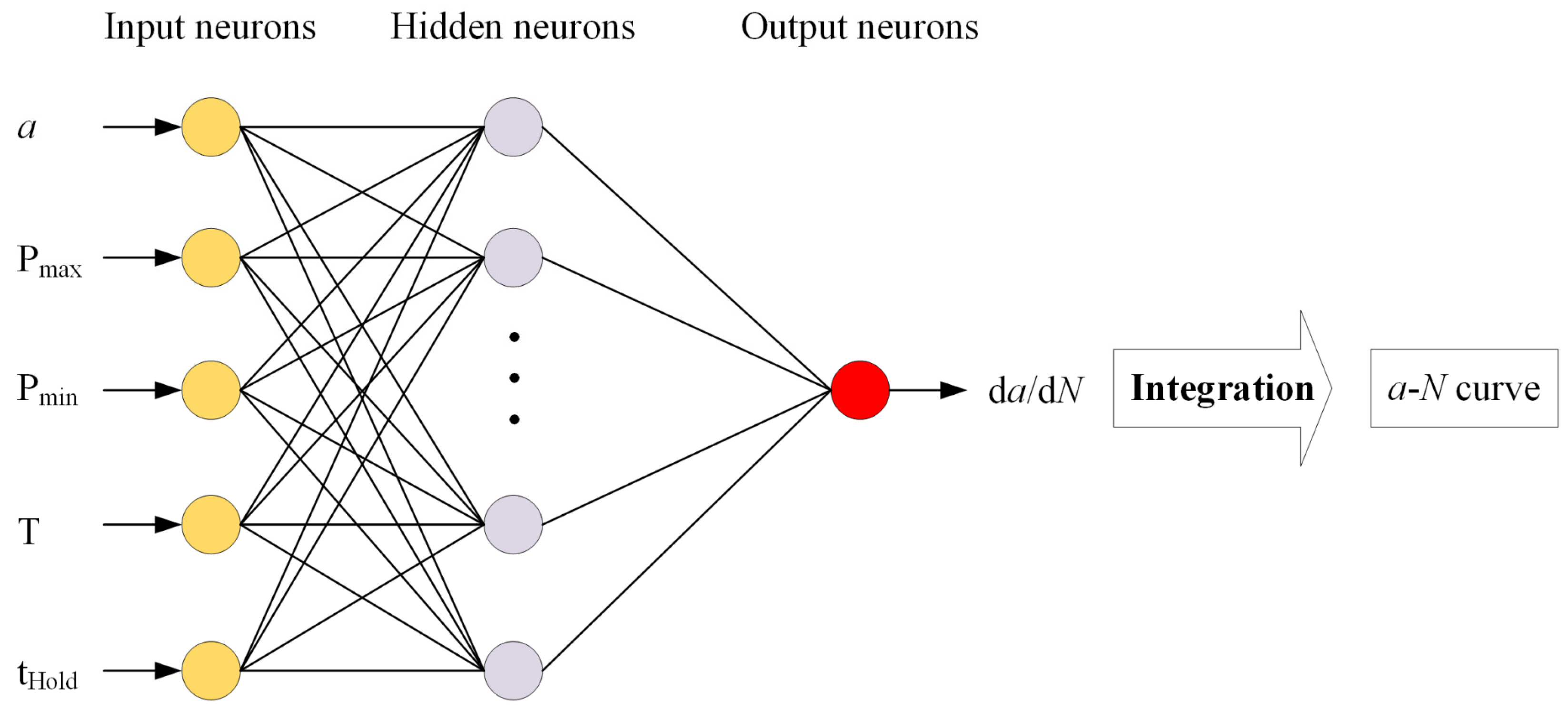
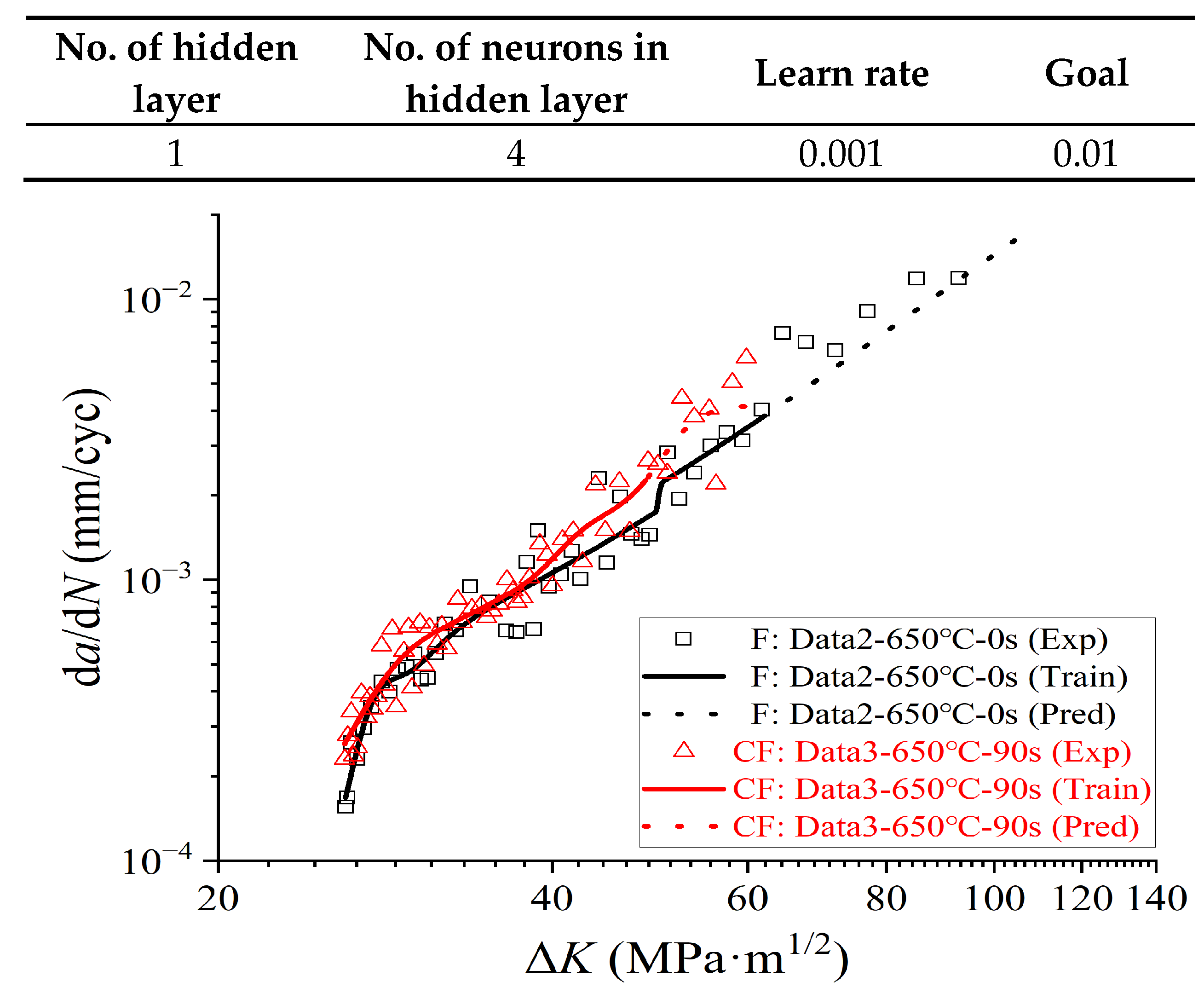
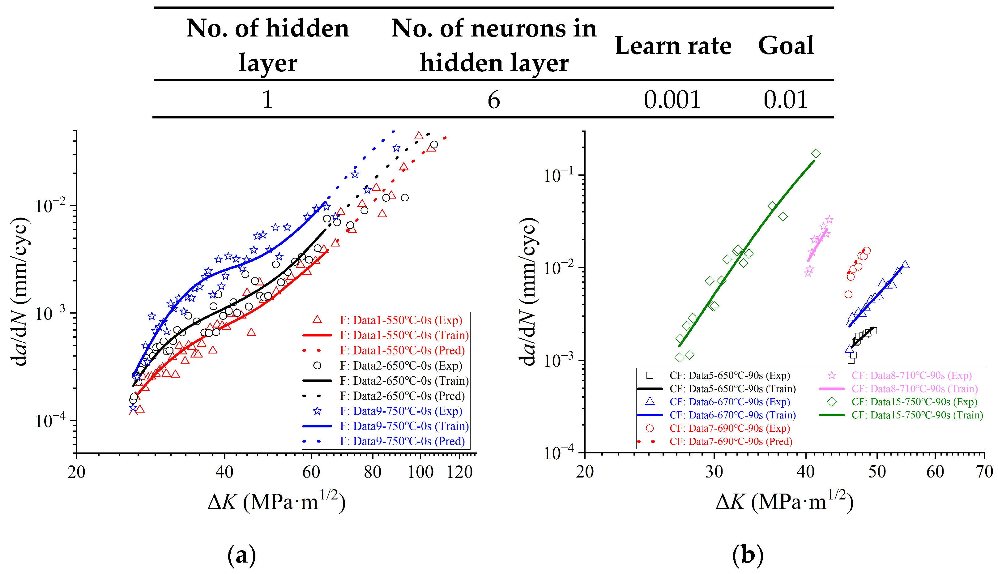
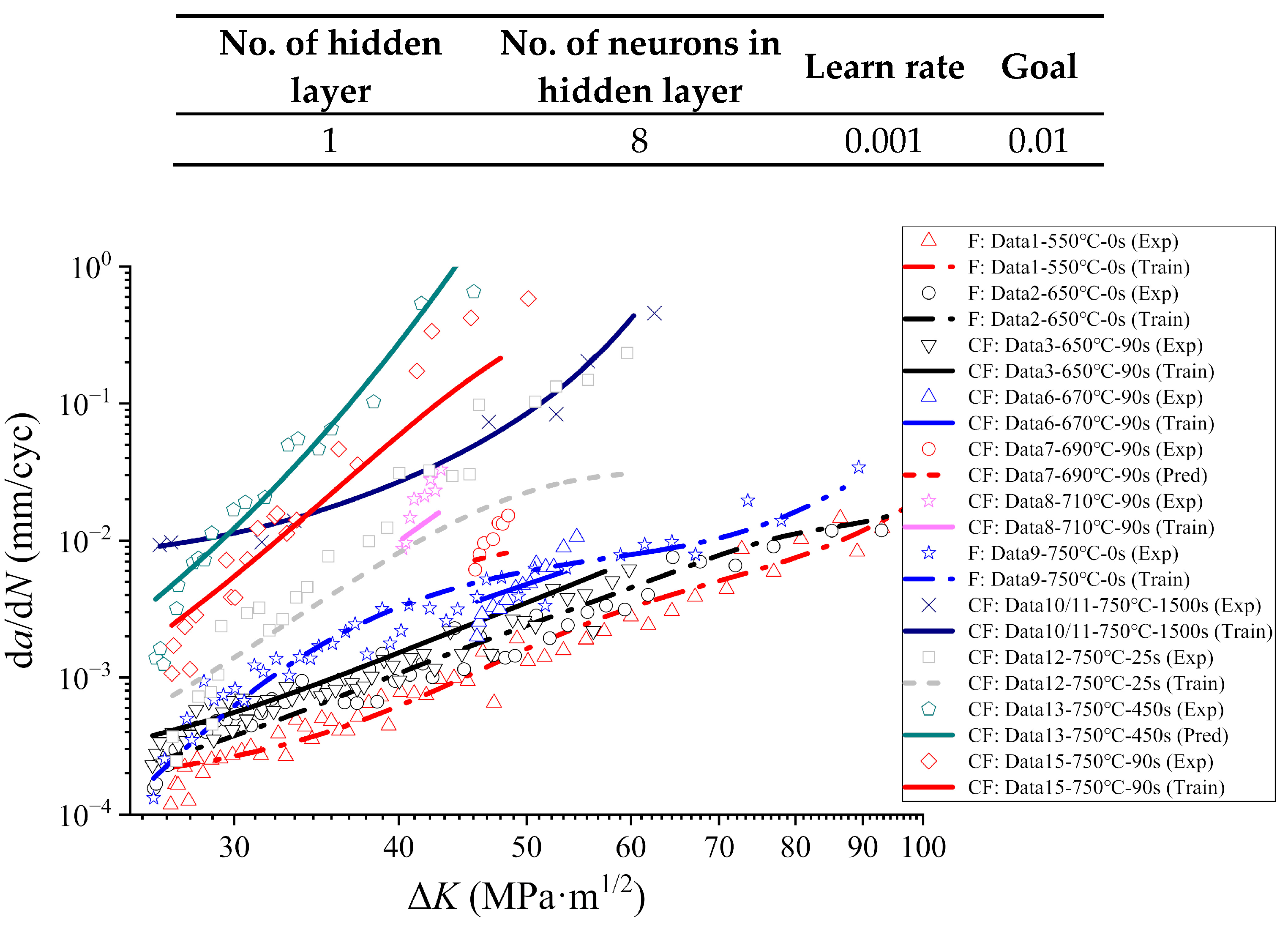
3.1. CG Prediction at Elevated Temperatures Based on CGR

The NNK method was used to predict CG at elevated temperatures for different cases.

Table 4. List of modelling cases using NNK method.

Method	NN Name	NN Input	NN Output	Dataset (Type of Testing Conditions: Train Data + Test Data)
NNK	NNK-K	Kmax, ΔK	da/dN	FCG: 80% Data 2 + 20% Data 2 CFCG: 80 % Data 3 + 20% Data 3
	NNK-KT	Kmax, ΔK, T		FCG with different T: 80% Data 1, 2, 9 + 20% Data 1, 2, 9 CFCG with same thold: Data 5, 6, 8, 15 + Data 7
	NNK-KTt	Kmax, ΔK, T, tHold		FCG + CFCG: Data 1–3, 6, 8–11, 13, 15 + Data 7, 12

Note: blue color and red color was used to mark the train dataset and test dataset respectively.

lists the information of NN for different cases in detail, including the NN structure and the corresponding dataset. It should be noted that the dataset is written as a format composed by type of testing conditions, train dataset and test dataset (marked by blue, black and red colors, respectively, in Table 4): the type of testing conditions is represented by the dataset name listed in Table 2; the train dataset is the set of experimental data points used to train the NN; the test dataset is the set of experimental data points, which cannot be obtained by interpolating the train dataset and will be compared with the NN-predicted results to verify the validation of NNK-K in the CG modelling at elevated temperatures. For example, FCG: 80% Data 2 + 20% Data 2 means that: the NNK-K was used to model the FCG under the specific service condition corresponding to Data 2; 80% data of Data 2 (ΔK < 61 MPa·m^1/2) was served as train dataset to train the NN; the remaining 20% data with larger ΔK (ΔK ≥ 61 MPa·m^1/2) was served as test dataset to be compared with the NN-predicted results.

Three types of NN structures (stated as NNK-K, NNK-KT and NNK-KTt) were used in the NNK method to model the CGR at elevated temperatures. NNK-K is designed to model the CGR under a specific service condition. About 80% data of Data 2 and 3 were learned by this NN, respectively. The obtained NN was used to predict the CGR corresponding the ΔK range for the remaining 20% data (ΔK > 46 MPa∙m^1/2 for Data 2, ΔK > 58 MPa∙m^1/2 for Data 3). Figure 5 shows the learning parameters of NN, the original data and modelling results. The black and red color mark the FCG (Data 2) and CFCG (Data 3) condition, respectively. It can be found that the slope of each curve decreases from a significantly high value to a stable value with the increase of the ΔK. This indicates the NN can clearly reflect the CGR characteristics at stage I and stage II. It can also be seen that black/red curves (both solid and dash curves) are within the range of rectangle/ triangle data points. This reflects that the NN results correspond well with the corresponding experimental data, thus predicting the CGR at elevated temperatures successfully. Above all, the NNK-K can be applied in CGR prediction at elevated temperatures to consider the single effect of CDF on the CGR of FCG and CFCG.

NNK-KT is designed to model the CGR under conditions with the same t_Hold (the interactive effect of CDF and T). This NN K-KT was applied to model the CGR based on a group of FCG data (t_Hold = 0) and a group of CFCG data (t_Hold = constant ≠ 0), respectively. It should be noted that six neurons were used in the hidden layer of NNK-KT, while there are four neurons in the hidden layer of NNK-K. More neurons were used because the NNK-KT need to consider the effect of one more factor (T) on the CGR prediction.

In terms of CGR prediction under the FCG condition, about 80% data of FCG dataset (Data 1, 2, 9) were learned together by NNK-KT. The evolution of CGR with ΔK under these three conditions were predicted by the obtained NNK-KT and compared with the remaining 20% data, see Figure 6a. It can be found that curves still correspond with the experimental data points but they do not correspond as well as that in Figure 5. The main deviations exist in the low ΔK area (ΔK < 30 MPa∙m^1/2), where the NN-predicted value is higher than the experimental value (around two times). It should be noted that this case is not a simple extrapolating by using 80% data to 20% data. These 20% data experimental data were used to validate the NNK-KT method by comparing them with the predicted results. The validated NN can be used to predict the FCG under other temperatures, like 670 °C. Because we do not have other group of FCG data to be compared with predicted results in this case, the predicted results under other temperatures are not shown here.

The NNK-KT was also used in the CGR prediction under CFCG conditions, see Figure 6b. Four groups of CFCG data with different temperatures (Data 5, 6, 8, 15) were used to train the NNK-KT. The CGR under another temperature was predicted by the obtained NNK-KT and compared with the experimental data (Data 7). Although the range of above data is short, they clearly reflect the relationship between da/dN and ΔK under different service conditions. As a result, it is useful to use these data to investigate the accuracy of the NN-based method in the CG prediction under different conditions in this research. A longer range of data will be measured and applied in CG prediction in future. It can be seen in Figure 6b that: the predicted values show the stage I and stage II CGR characteristics; differences between curves and experimental data in Figure 6b are remarkable at the stage I of CG (lower ΔK) but small at the stage II of CG (higher ΔK); the NN-predicted da/dN is higher than the experimental value at the stage I of CG. These characteristics are the same as for that of the CGR prediction under FCG conditions (see Figure 6a). These indicate that the NNK-KT can be applied in the CGR prediction under the interactive effect of CDF and T for both FCG and CFCG. It predicts CGR at the higher ΔK area for each case (stage II of CG) very well but overestimates CGR at the lower ΔK area for each case (stage I of CG). This overestimation may result in the lower predicted value of CG life in CG prediction based on CGR.

NNK-KTt is designed to model the CGR under general conditions (with the interactive effect of CDF, T and t_Hold). More neurons were used in its hidden layer (eight neurons in total) than that of NNK-KT in order to consider the effect of added factor (t_Hold). Experimental da/dN-ΔK data for all combination of T and t_Hold listed in Table 2 (Data 1–3, 6–13, 15) were used in this research to train and test this NN. Figure 7 shows the predicted results of obtained NNK-KTt and related experimental data. The predicted results corresponding to train data under the same t_Hold were marked by the same type of curves. For example, dot curves are used to mark the Data with t_Hold = 0 s. The predicted results corresponding to test data (Data 7, 13) were marked by solid curves. It can be found in Figure 7 that maximum differences between all types of curves and experimental data are about twice that of the smaller da/dN under a same ΔK. This can be accepted in the CGR prediction and reflects the usefulness of applying NNK-KTt in the CGR prediction with the interactive effect of CDF, T and t_Hold.

Based on the CGR predicted in this section, the evolution of CG (a-N curves) under different conditions was modelled. It should be noted that this research is focused on the relationship between the a and N rather than the modelling of the crack growth life. Therefore, there is not a unified stop criteria for the modelling. When the crack length is relatively long or reaches the maximum crack length of the corresponding experimental data, the prediction will be stopped. The modelling results of CG are shown in Figure 8 and Figure 9, where Figure 8a–c and Figure 9 are integrated results of Figure 5, Figure 6a, Figure 6b and Figure 7, respectively. It can be found in these images that all predicted results (solid curves) correspond well with the experimental data (data points) at the start of CG but the difference between them (deviation of CG prediction) increase with the increase of cycle numbers N. For example, the difference of crack length between the blue solid curve and black rectangle in Figure 8a is 0 mm at N = 0 cycle, while the value of this difference increases to over 4 mm at N = 15,447 cycle. This indicates the accumulation of deviation in the CG prediction based on CGR. As a result, the accuracy of the NNK method in the CG prediction under different conditions is relatively high when the CG life is relative short (see N ≤ 800 cycles in Figure 9b). However, the accuracy of this method becomes low when CG life is relative long (see N > 5000 cycle in Figure 9a). In summary, this “Indirect” NN-based method is more appropriate to be applied in CG prediction at elevated temperatures with short CG life.

3.2. CG Prediction at Elevated Temperatures Using NN-Based Method Established at Room Temperature

The RNN and NNIL are two types of “direct” NN-based CG prediction methods, which directly build the relationship between N and a by using NN. They were established at room temperature but were used to model the CG at elevated temperatures in this research.

Table 5. List of modelling cases using RNN and NNIL method.

Method	NN Name	NN Input	NN Output	Dataset (Type of Testing Conditions: Train Data + Test Data)
RNN	RNN-N	N	a	FCG: 45% Data 2 + 55% Data 2 FCG: 65% Data 2 + 35% Data 2 FCG: 85% Data 2 + 15% Data 2 CFCG: 65% Data 3 + 35% Data 3
NNIL	NNIL-N	N, ΔN′	a, Δa′	FCG: 80% Data 2 + 20% Data 2 CFCG: 80% Data 3 + 20% Data 3

lists their NN structure and the corresponding dataset, including the type of testing conditions (marked by blue color), train data (marked by black color) and test data (marked by red color). The design of these dataset is to reflect the problem of applying these methods into the CG prediction at elevated temperatures.

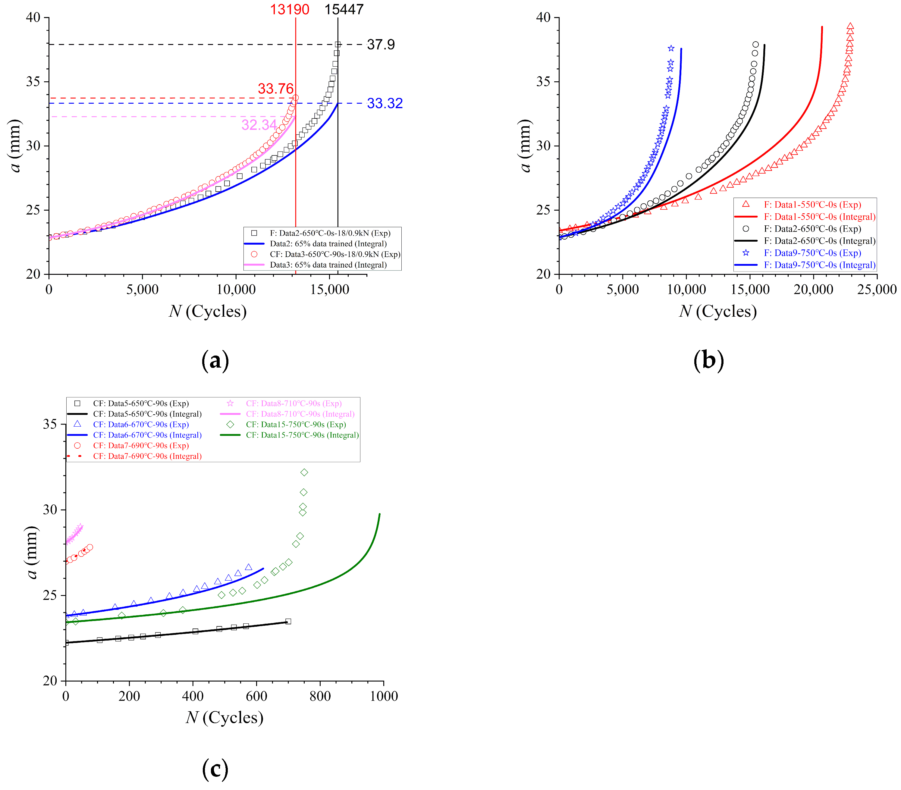
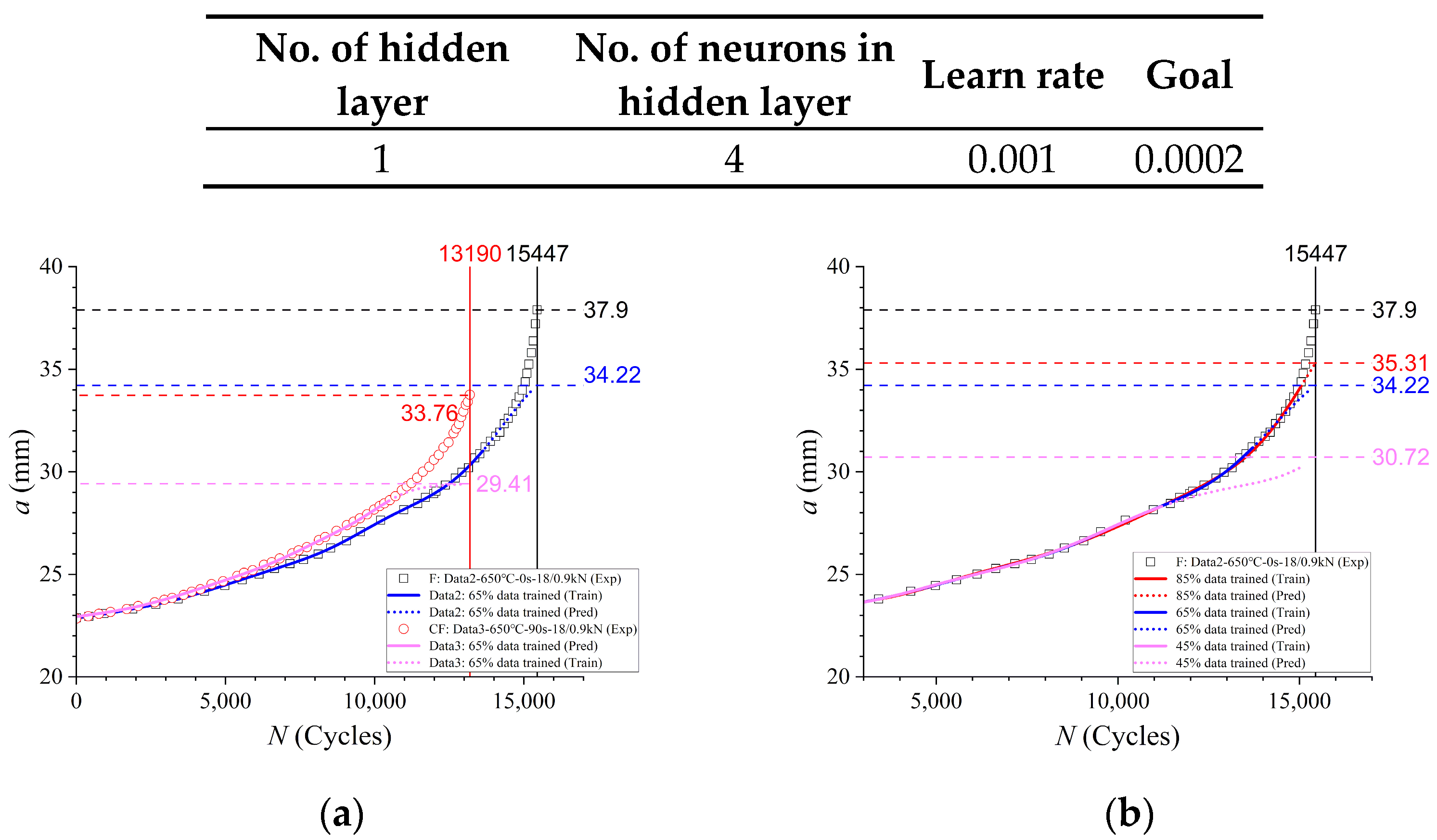
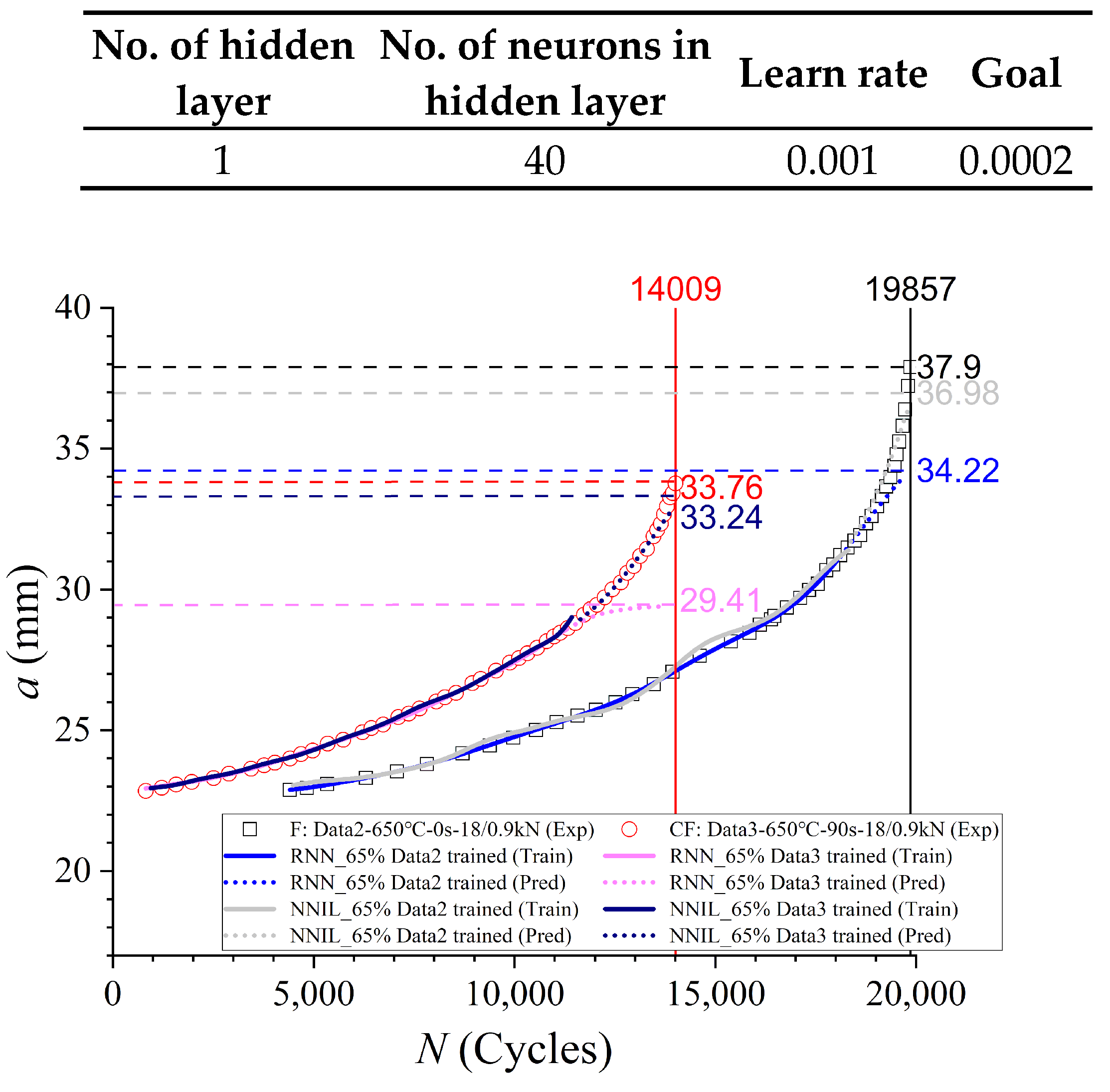
3.2.1. Prediction Using the Basic NN Method

The RNN is the traditional NN-based method modelling the CG under a specific service condition at room temperature. Its input and output parameter are N and a, respectively. This method was applied in the FCG and CFCG prediction in this section.

About 65% data of FCG data measured under a specific condition (Data 2) were learned by the RNN to train the NN. The obtained NN was used to predict the a-N curve corresponding to the remaining 35% data (test data with the N ranging from 13,690 to 15,447 cycles). Figure 10a shows the predicted results (FCG prediction), where the predicted results for the train data and test data were marked by the blue solid curve and blue dash curve, respectively. It can be found that the blue solid curve corresponds well with the experimental data (marked by black rectangles) in the range of N from 0 to 13,690 cycles. However, the difference between the blue dash curve and black rectangles is significant: the predicted value is smaller than the test data; the difference between the predicted value and test data increases from around 0 mm at 13,690 cycles to over 3 mm at 15,447 cycles (37.9 − 34.22 = 3.68 mm). These characteristics can also be seen in the CFCG prediction (Data 3 in Figure 10a), where the difference between the predicted value and experimental value increases from around 0 mm at 10,694 cycles to over 4 mm at 13,190 cycles.

The effect of percentage of data selected to train the RNN on the predicted results were also investigated. About 45%, 65% and 85% data of Data 2 (train data) were learned by the RNN to train the NN, see Figure 10b. It can be found that differences between predicted results (dash curves) and experimental data (black rectangle) decreases with the increase of the percentage of selected train data. It decreases to around 2.6 mm at 15,447 cycles for 85% selected train data. This indicates that increasing the percentage of data selected to train NN can improve the above-mentioned deviation of predicted value in the CG prediction at elevated temperatures. However, the predicted results were not well although over 85% data were selected. Therefore, RNN cannot predict the CG at elevated temperature very well.

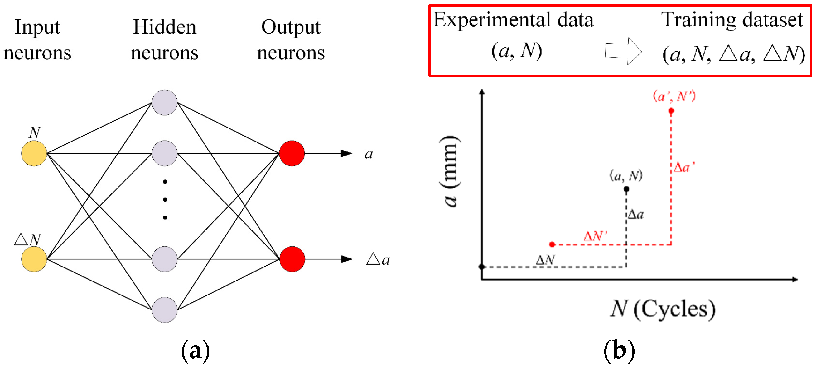
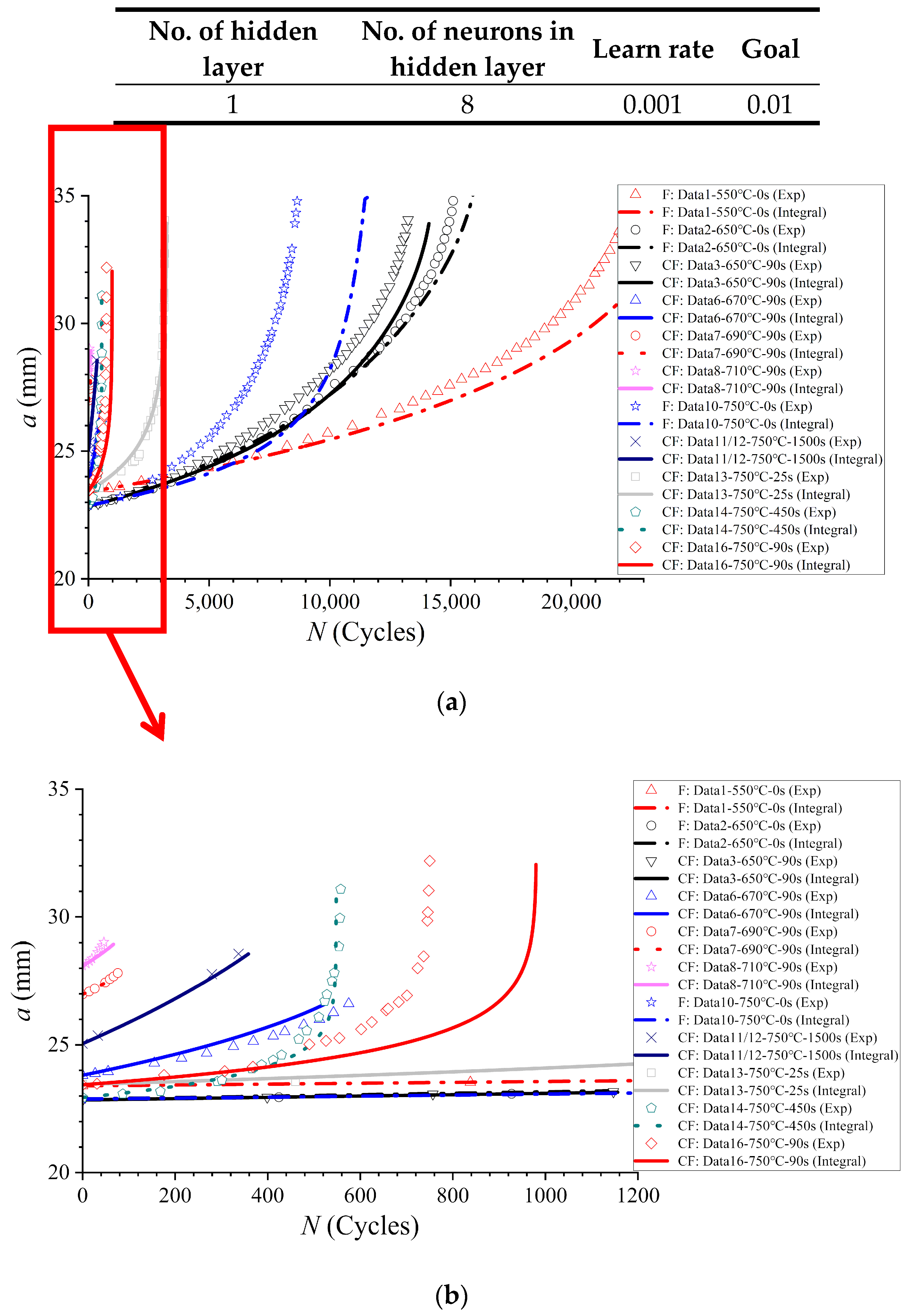
3.2.2. Prediction Using NN-Based Increment Learning Scheme

The NNIL method was applied in the FCG and CFCG prediction. Two train datasets were generated by about 65% data of Data 2 and Data 3, respectively, using the method stated in Figure 3b. These generated datasets were used to train NNIL for the prediction of FCG and CFCG. Figure 11 shows predicted results of obtained NNILs, where the navy dash curve and the gray dash curve are predicted results for test dataset in FCG and CFCG prediction, respectively. The significant decrease of predicted deviations can be found for both FCG prediction (from over 3 mm to around 0.9 mm at 19,857 cycles) and CFCG prediction (from over 4 mm to around 0.5 mm at 14,009 cycles). This shows the potential of the NNIL method in the improvement of CG prediction at elevated temperatures.

However, the current structure of NNIL limits the further application of this NN in CG prediction. The NN structure of NNIL cannot be used to consider the effect of multiple factors on the CG directly because its input parameters (N and ΔN′) are not essential parameters controlling CG. For example, the a-N curve will change significantly with the change of the initial crack length, although the service condition of CG is the same. This means that the N cannot determine the CG at elevated temperatures together with other affecting factors T, t_hold, P_max and P_min. This issue will be solved in Section 3.3 by developing an amended NNIL method. The consideration of the effect of a₀ is because the a₀ of a-N curves measured in repeatability tests (same sample configures and loading conditions) is different. This difference of a₀ is due to the difference of pre-crack and reading strategy.

3.3. CG prediction at Elevated Temperature with Amended NNIL Method (ENNIL Method)

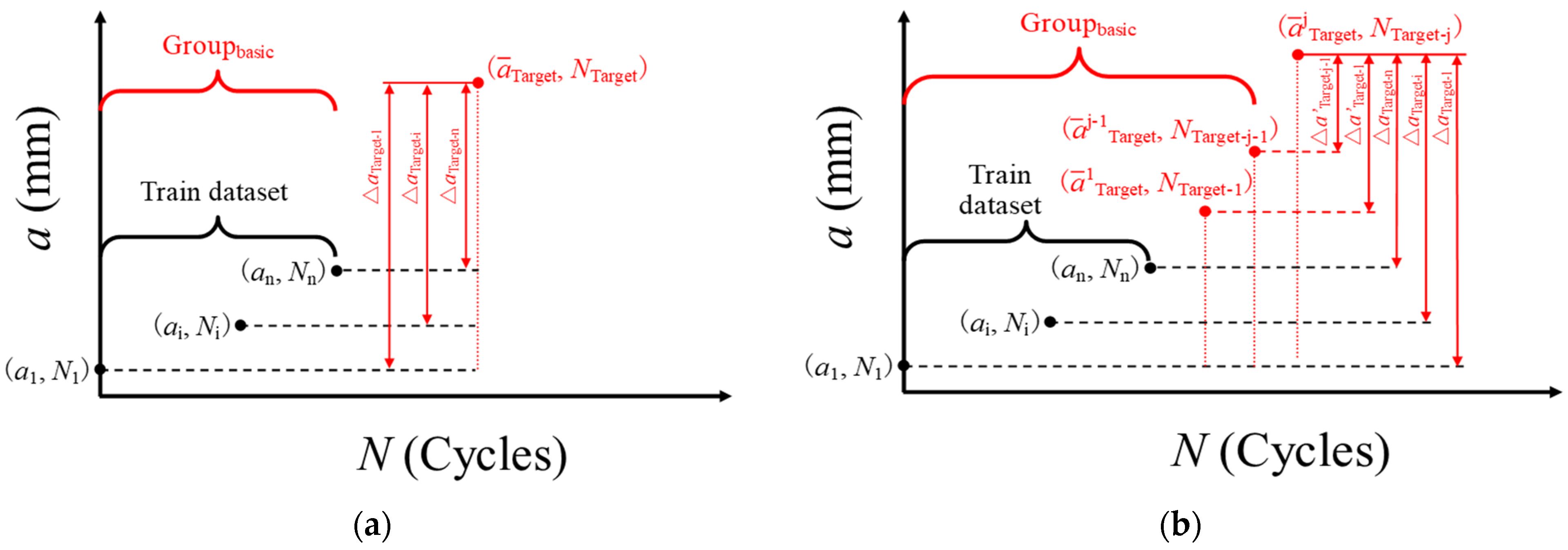
The ENNIL is an amended NNIL method developed in this research, where a, ΔN′ replace N, ΔN′ to serve as the basic input parameters and the Δa becomes the only one output parameter. Bringing the crack length into the input parameters is because a can determine the CG at specific service conditions together with other affecting factors, such as T, t_hold, P_max and P_min. In order to check the predicted results of this ENNIL method, CG at elevated temperatures under a series of different cases were investigated in this research.

Table 6. List of modelling cases using ENNIL method.

Method	NN Name	NN Input	NN Output	Dataset (Type of Testing Conditions: Train Data + Test Data)
ENNIL	ENNIL-a	a, ΔN′	Δa	F: 80% Data 2 + 20%Data 2 CF: 80% Data 3 + 20%Data 3
	ENNIL-aP	a, ΔN′, PMax, PMin		CF with effects of loads: 80% Data 3, 4 + 20%Data 3, 4
	ENNIL-aPT	a, ΔN′, PMax, PMin, T		CF with effect of loads and temperature: Data 5, 6, 8, 15 +Data7
	ENNIL-aPTt	a, ΔN′, PMax, PMin, T, tHold		F + CF: Data 1–6, 8–12, 14–16 +Data 7, 13

lists their NN structure and the corresponding dataset for these cases, including type of testing conditions (marked by blue color), train dataset (marked by black color) and test dataset (marked by red color).

It should be noted that the way to construct dataset for predicting the crack length of the target testing point is the basis in the CG prediction using the ENNIL method. Therefore, it was investigated before applying different NN structures of ENNIL on CG prediction at elevated temperatures. There are two ways that were investigated in total.

The first way is the one used in the NNIL method (“Unmove” way), see Figure 12a. This prediction was carried out based on all data points with the same P_Max, P_Min, T and t_Hold in train dataset (the group of these data points were stated as Group_basic). There are two steps to follow in this way.

(a)

The crack lengths at the N_Target of the target testing point were predicted by using each data point in Group_basic, respectively. The predicted crack length using the i^th point of Group_basic was stated as a_Target−i, whose value was calculated by Equation (3):

$$a_{\mathrm{Target}-\mathrm{i}}=a_{\mathrm{i}}+\Delta a_{\mathrm{Target}-\mathrm{i}}$$

(3)

where a_i is the crack length of ith point, Δa_Target−i is the increment crack length calculated by inputting a_i and N_Target − N_i into the NN of the ENNIL method.

(b)

The mean value of all predicted crack lengths were calculated by Equation (4):

$${\overline{a}}_{\mathrm{Target}}=1/n\times {{\displaystyle \sum }}_{i=1}^n{a}_{\mathrm{Target}}=1/n\times {{\displaystyle \sum }}_{i=1}^n\left(a_{\mathrm{i}}+\Delta a_{\mathrm{Target}-\mathrm{i}}\right)$$

(4)

where n is the total number of data points in Group_basic. This obtained mean value ${\overline{a}}_{\mathrm{Target}}$ is the final predicted crack length of the target testing point in the “Unmove” way.

The other way is the “Move” way, demonstrated in Figure 12b. $\left({\overline{a}}_{\mathrm{Target}}^j,N_{\mathrm{Target}}^j\right)$ represents the coordinate value of jth predicted data point A_j. Group_j represents the dataset used to predict this data point A_j. The detailed procedure is as follows:

(a)

For the first predicted data point, the “Unmove” way was used to predict the ${\overline{a}}_{\mathrm{Target}}^1$ corresponding to $N_{\mathrm{Target}}^1$ based on the train dataset (Group₁).

(b)

For other predicted data points, the crack length is also calculated using the “Unmove” way, but the Group_basic used in the calculation of Equation (1) and (2) is composed by Group₁ and previously predicted data points. For example, the Group_basic in the predition of jth data point is composed by Group₁ and (A₁, A₂, …, A_j-1). The equation for the ${\overline{a}}_{\mathrm{Target}}^j$ is

$${\overline{a}}_{\mathrm{Target}}^j=1/\left(n_0+j-1\right)\times \left[{{\displaystyle \sum }}_{i=1}^{n_0}\left(a_{\mathrm{i}}+\Delta a_{\mathrm{Target}-\mathrm{i}}\right)+{{\displaystyle \sum }}_{i=1}^{j-1}\left({\overline{a}}_{\mathrm{Target}}^i+\Delta {a^{\prime }}_{\mathrm{Target}-\mathrm{i}}\right)\right]$$

(5)

where n₀ is the number of data points in Group₁, $\Delta {a^{\prime }}_{\mathrm{Target}-\mathrm{i}}$ is the increment crack length calculated by inputting ${\overline{a}}_{\mathrm{Target}}^i$ and $N_{\mathrm{Target}}^j-N_{\mathrm{Target}}^i$ into the NN of the ENNIL method.

These two ways were applied into the FCG prediction under a specific service condition (Data 2) to compare their predicting accuracy. The NN structure used in this prediction is ENNIL-a. Predicted results are shown in Figure 13, where the 60% and 85% data of Data 2 were used to train the ENNIL-a, respectively. It can be found in both Figure 13a,b that the predicted results of ENNIL-a with the “Move” way (marked by blue dash curves) are closer to the experimental data (marked by black rectangles) than that of ENNIL-a with “Unmove” way (marked by red dash curves). This indicates that the predicting deviation of the “Move” way (below 1 mm at 15,447 cycles) is remarkable smaller than that of the previous “Unmove” way (over 3 mm at 15,447 cycles). The possible reason for this may be that the “Move” way can consider the increased slope of a with the increase of N better because it used predicted data with bigger slope in the CG prediction for bigger N. Therefore, the “Move” way is more appropriate to be applied into the CG prediction at elevated temperatures.

The ENNIL method with the “Move” way was applied to analyze the case which cannot be modelled by the NNIL method (demonstrated in the end of Section 3.2.2). A total of 60% data of Data 3 were used to the train the ENNIL-a in this CFCG prediction. Figure 14 shows the predicted results, where predicted results for train dataset and test dataset are marked by a solid curve and a dash curve, respectively. It can be found that all curves correspond well with the experimental data. This means that using a to replace N in the NN of the NNIL method (a, ΔN as basic input parameters of NN in ENNIL method) can determine CG characteristics (a-N curves for all initial length) under a specific service condition.

The CG with the effect of multiple service conditions were predicted by the ENNIL method with the “Move” way. Parameters around service conditions were added in NN as input parameters. P_Max and P_Min were added first (ENNIL-aP) to consider the effect of loads on the CG prediction. Figure 15a shows a CG prediction case by using the ENNIL method with ENNIL-aP, where ENNIL-aP were trained by two groups of data measured under different loads (Data 3, Data 4). It can be seen that the predicted results for both train dataset and test dataset (solid curves and dash curves) correspond well with the experimental data (differences below 0.2 mm at the same N). T were further added in the NN of the ENNIL method (ENNIL-aPT). Figure 15b shows a CG prediction case by using the ENNIL method with ENNIL-aPT. In this case, four groups of experimental data measured under different loads and temperatures (Data 5, 6, 8, 15) were used to train NN. The obtained NN were used to predict the CG for another service condition (corresponding to the test dataset Data 7). The input of this prediction includes the a₀ and parameters describing the service conditions_. It can be seen in Figure 15b that differences between predicted results (solid/dash curves) and corresponding experimental data (discrete points marked by different shapes) are minor (below 0.5 mm). The above comparisons verify the validation of the ENNIL method in the CG prediction at elevated temperatures.

This ENNIL method was also applied in the CG prediction under more general conditions (interactive effect of P_Max, P_Min, T and t_Hold). This prediction uses ENNIL-aPTt and all experimental data listed in Table 2, where Data 7, 13 compose test dataset and other data (Data 1–6, 8–12, 14–16) compose the train dataset. The number of neurons in the hidden layer was increased from 40 to 120 in this prediction because there are more input parameters. Figure 16 shows the predicted results for this case, where Figure 16b is the zoom-in image of Figure 16a for the narrow range of N (0–1000 cycles). It can be seen that: for CG with longer CG life (N > 1000 cycles at a = 32 mm), predicted results corresponds well with experimental data (maximum deviation below 1 mm); for CG with shorter CG life (N ≤ 1000 cycles at a = 32 mm), predicted results can coarsely describe the increase of a with the increase of N, while predicted results cannot describe the rapid increase in slope of curves for longer crack length; the maximum deviation for both test dataset and train dataset with the shorter CG life is around 3 mm. These indicate that the ENNIL method can be used in the CG prediction under general conditions and give perfectly predicted results for cases with relatively long CG life. However, the predicted accuracy of this method for CG with relatively short CG life need to be further improved. Increasing the CG data with the short CG life to train NN and taking log of N for all data before training NN may be the possible solution. They will be investigated in the future.

It should be noted that the NNK method presented in Section 3.1 shows high accuracy in CG prediction with relatively short CG life, but low accuracy in CG prediction with relative long CG life. This is opposite to the ENNIL method. It means that the combination of these two methods may be an effective way to achieve high accuracy in CG prediction at elevated temperatures. The detailed solution maybe: (a) training NN for the NNK methods and the ENNIL methods, respectively, by using same train dataset; (b) using the NNK methods to predict CG at elevated temperatures with shorter CG life and (c) using the ENNIL methods to predict CG at elevated temperatures with the longer CG life.

4. Conclusions

The neutral network was applied in CG prediction at elevated temperatures in this research. Both the “direct” and “indirect” NN-based methods were built by extending the NN-based methods performing well at room temperature to the CG prediction at elevated temperatures. The following conclusions were drawn:

(a)

NN with the input of CDF and other parameters describing service condition can be applied in CGR prediction at elevated temperatures. The CGR at the higher ΔK area are predicted well by this NN but CGR at the lower ΔK area are usually overestimated.

(b)

The RNN and NNIL cannot be directly used in CG prediction at elevated temperatures. An important reason for this is that N cannot determine the CG at elevated temperatures together with other affecting factors.

(c)

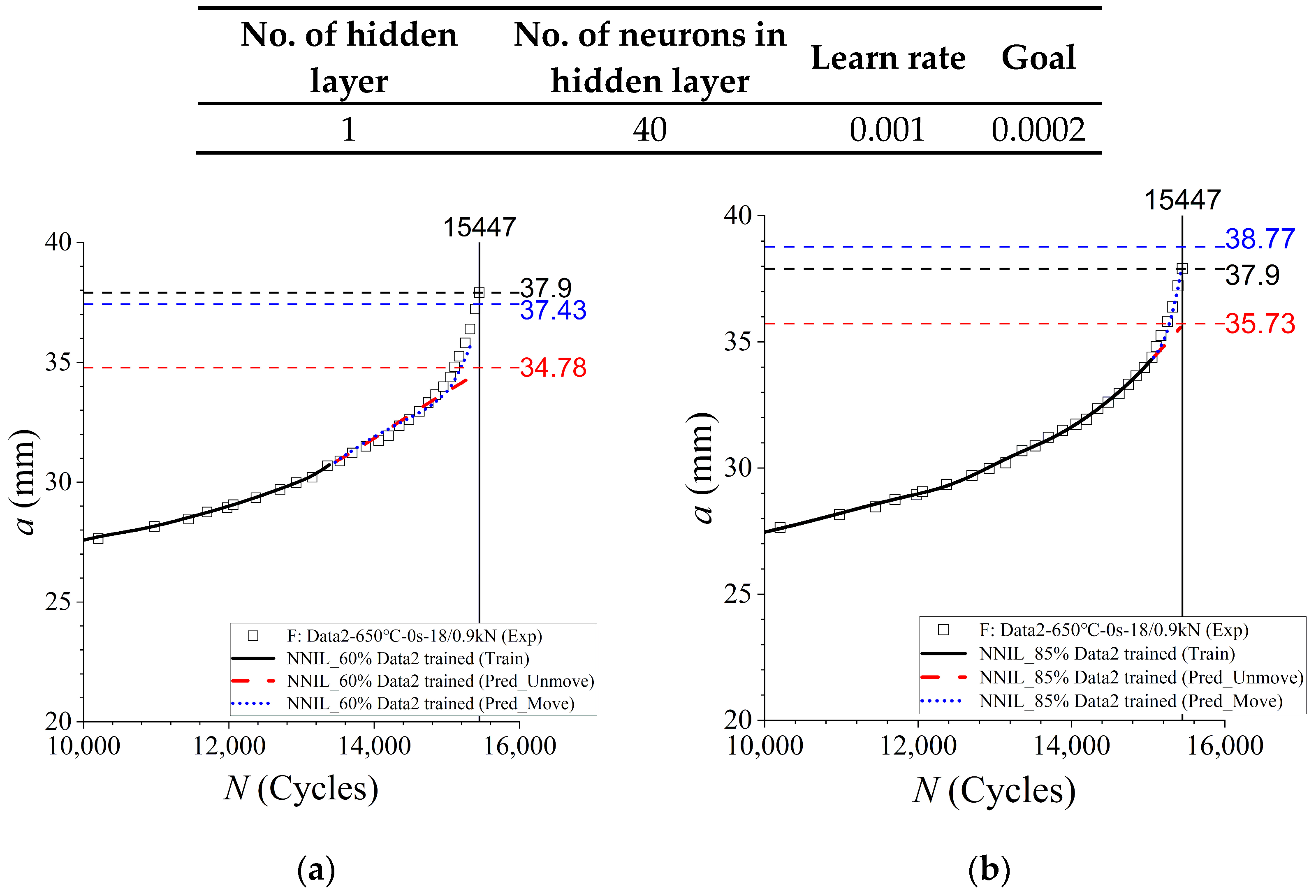
The ENNIL method was developed in this research, where a, ΔN′ replace N, ΔN′ in the NNIL method to serve as the basic input parameters and the Δa becomes the only one output parameter. This method makes the increment schedule can be applied in the CG prediction under general conditions, thus getting over the shortage of using BPNN to model the CG (not good at training on small dataset).

(d)

The ENNIL method gives perfectly predicted results for cases with relatively long CG life, while the predicted accuracy of this method for CG with relatively short CG life need to be further improved. However, the NNK method shows high accuracy in CG prediction with relatively short CG life, but low accuracy in CG prediction with relative long CG life. The combination of these two methods may be an effective way to achieve high accuracy in CG prediction at elevated temperatures.

References

1. Shlyannikov, V.; Iltchenko, B.; Stepanov, N. Fracture analysis of turbine disks and computational–experimental background of the operational decisions. Eng. Fail. Anal. 2001, 8, 461–475. [Google Scholar] [CrossRef]
2. Payten, W.M.; Wei, T.; Snowden, K.U.; Bendeich, P.; Law, M.; Charman, D. Crack initiation and crack growth assessment of a high pressure steam chest. Int. J. Press. Vessel. Pip. 2011, 88, 34–44. [Google Scholar] [CrossRef]
3. Narasimhachary, S.; Saxena, A. Crack growth behavior of 9Cr−1Mo (P91) steel under creep–fatigue conditions. Int. J. Fatigue 2013, 56, 106–113. [Google Scholar] [CrossRef]
4. Shlyannikov, V. Creep–fatigue crack growth rate prediction based on fracture damage zone models. Eng. Fract. Mech. 2019, 214, 449–463. [Google Scholar] [CrossRef]
5. Tong, J.; Dalby, S.; Byrne, J.; Henderson, M.B.; Hardy, M.C. Creep, fatigue and oxidation in crack growth in advanced nickel base superalloys. Int. J. Fatigue 2001, 23, 897–902. [Google Scholar] [CrossRef]
6. Onofrio, G.; Osinkolu, G.A.; Marchionni, M. Fatigue crack growth of UDIMET 720 Li superalloy at elevated temperature. Int. J. Fatigue 2001, 23, 887–895. [Google Scholar] [CrossRef]
7. Pairs, P.; Erdogan, F. A critical analysis of crack propagation laws. J. Basic Eng. 1963, 85, 528–534. [Google Scholar] [CrossRef]
8. Djavanroodi, F. Creep-Fatigue Crack Growth Interaction in Nickel Base Supper Alloy. Am. J. Appl. Sci. 2008, 5, 454–460. [Google Scholar] [CrossRef] [Green Version]
9. Whittaker, M.; Harrison, W.; Hurley, P.; Williams, S. Modelling the behaviour of titanium alloys at high temperature for gas turbine applications. Mater. Sci. Eng. A 2010, 527, 4365–4372. [Google Scholar] [CrossRef] [Green Version]
10. Grover, P.S.; Saxena, A. Modelling the effect of creep–fatigue interaction on crack growth. Fatigue Fract. Eng. Mater. Struct. 1999, 22, 111–122. [Google Scholar] [CrossRef]
11. Shlyannikov, V.; Tumanov, A.; Boychenko, N. A creep stress intensity factor approach to creep–fatigue crack growth. Eng. Fract. Mech. 2015, 142, 201–219. [Google Scholar] [CrossRef]
12. Yang, H.; Bao, R.; Zhang, J. An interaction crack growth model for creep-brittle superalloys with high temperature dwell time. Eng. Fract. Mech. 2014, 124–125, 112–120. [Google Scholar] [CrossRef]
13. Lepore, M.A.; Maligno, A.R.; Berto, F. A unified approach to simulate the creep-fatigue crack growth in P91 steel at elevated temperature under SSY and SSC conditions. Eng. Fail. Anal. 2021, 127, 105569. [Google Scholar] [CrossRef]
14. Xu, L.; Zhao, L.; Gao, Z.; Han, Y. A novel creep–fatigue interaction damage model with the stress effect to simulate the creep–fatigue crack growth behavior. Int. J. Mech. 2017, 130, 143–153. [Google Scholar] [CrossRef]
15. Piard, A.; Gamby, D.; Carbou, C.; Mendez, J. A numerical simulation of creep–fatigue crack growth in nickel-base superalloys. Eng. Fract. Mech. 2004, 71, 2299–2317. [Google Scholar] [CrossRef]
16. Bouvard, J.; Chaboche, J.; Feyel, F.; Gallerneau, F. A cohesive zone model for fatigue and creep–fatigue crack growth in single crystal superalloys. Int. J. Fatigue 2009, 31, 868–879. [Google Scholar] [CrossRef]
17. Morse, L.; Khodaei, Z.S.; Aliabadi, M. A multi-fidelity modelling approach to the statistical inference of the equivalent initial flaw size distribution for multiple-site damage. Int. J. Fatigue 2018, 120, 329–341. [Google Scholar] [CrossRef]
18. Zio, E.; Di Maio, F. Fatigue crack growth estimation by relevance vector machine. Expert Syst. Appl. 2012, 39, 10681–10692. [Google Scholar] [CrossRef]
19. Hu, D.; Su, X.; Liu, X.; Mao, J.; Shan, X.; Wang, R. Bayesian-based probabilistic fatigue crack growth evaluation combined with machine-learning-assisted GPR. Eng. Fract. Mech. 2020, 229, 106933. [Google Scholar] [CrossRef]
20. Mortazavi, S.; Ince, A. An artificial neural network modeling approach for short and long fatigue crack propagation. Comput. Mater. Sci. 2020, 185, 109962. [Google Scholar] [CrossRef]
21. Mohanty, J.; Verma, B.; Parhi, D.; Ray, P. Application of artificial neural network for predicting fatigue crack propagation life of aluminum alloys. Arch. Comput. Mater. Sci. Surf. Eng. 2009, 1, 133–138. [Google Scholar]
22. Zhang, W.; Bao, Z.; Jiang, S.; He, J. An Artificial Neural Network-Based Algorithm for Evaluation of Fatigue Crack Propagation Considering Nonlinear Damage Accumulation. Materials 2016, 9, 483. [Google Scholar] [CrossRef] [PubMed] [Green Version]
23. Pidaparti, R.M.V.; Palakal, M.J. Neural network approach to fatigue-crack-growth predictions under aircraft spectrum loadings. J. Aircr. 1995, 32, 825–831. [Google Scholar] [CrossRef]
24. Do, D.; Lee, J.; Hung, N. Fast evaluation of crack growth path using time series forecasting. Eng. Fract. Mech. 2019, 218, 106567. [Google Scholar] [CrossRef]
25. Ma, X.; He, X.; Tu, Z. Prediction of fatigue–crack growth with neural network-based increment learning scheme. Eng. Fract. Mech. 2020, 241, 107402. [Google Scholar] [CrossRef]
26. Yang, H.; Bao, R.; Zhang, J.; Peng, L.; Fei, B. Crack growth behaviour of a nickel-based powder metallurgy superalloy under elevated temperature. Int. J. Fatigue 2011, 33, 632–641. [Google Scholar] [CrossRef]
27. Bao, R.; Yang, H.; Zhang, J.; Peng, L.; Fei, B. Fatigue crack growth measurement in a superalloy at elevated temperature. Int. J. Fatigue 2013, 47, 189–195. [Google Scholar] [CrossRef]
28. Yang, H. Sub-Critical Fatigue Crack Growth Behaviour Analysis for a P/M Superalloy under Elevated Temperature. Ph.D. Thesis, Beihang University, Beijing, China, 2010. [Google Scholar]
29. Zhang, Y.; Zhang, Y.; Zhang, N.; Jia, J. Heat treatment processes and microstructure and properties research on P/M superalloy FGH97. Chin. J. Aero. Mater. 2008, 28, 5–9. [Google Scholar]
30. ASTM E647-08; Standard Test Method for Measurement of Fatigue Crack Growth Rates. ASTM Committee: Seattle, WA, USA, 2008.
Figure 1. (a) Configuration of CT specimens, (b) 1.5 s−1.5 s triangular waveforms, and (c) trapezoidal waveforms corresponding to the dwelling time (tHold).
Aerospace 09 00600 g001
Figure 2. Schematic diagram of NNK method.
Aerospace 09 00600 g002
Figure 3. (a) Schematic diagram of NN structure for NNIL method and (b) the way to construct dataset during testing process.
Aerospace 09 00600 g003
Figure 4. Schematic diagram of NN structure for ENNIL method.
Aerospace 09 00600 g004
Figure 5. Prediction of the evolution of da/dN with ΔK under fatigue condition (Data2–650 °C-0s-18/0.9 kN) and creep-fatigue condition (Data3–650 °C-90s-18/0.9 kN).
Aerospace 09 00600 g005
Figure 6. Prediction of the evolution of da/dN with ΔK under (a) fatigue condition with different elevated temperatures (550/650/750 °C-0s-18/0.9 kN) and (b) creep-fatigue condition with different elevated temperatures (650–750 °C).
Aerospace 09 00600 g006
Figure 7. Prediction of the evolution of da/dN with ΔK under different elevated temperatures (650–750 °C) and different holding times (thold from 0 to 1500 s).
Aerospace 09 00600 g007
Figure 8. Prediction of a-N curves using NNK method for: (a) fatigue condition (Data2–650 °C-0s-18/0.9 kN) and creep-fatigue condition (Data3–650 °C-90s-18/0.9 kN), respectively; (b) fatigue condition with different elevated temperatures (550/650/750 °C-0s-18/0.9 kN); and (c) creep-fatigue condition with different elevated temperatures (650–750 °C).
Aerospace 09 00600 g008
Figure 9. Prediction of a-N curves using NNK method for conditions with different elevated temperatures (650–750 °C) and different holding times (thold from 0 to 1500 s).
Aerospace 09 00600 g009
Figure 10. Prediction of a-N curves using basic scheme (RNN) for (a) Data2 and Data3, respectively; (b) Data2 with various of trained data percentage.
Aerospace 09 00600 g010
Figure 11. a-N curves prediction using RNN and NNIL scheme for Data2 and Data3, respectively.
Aerospace 09 00600 g011
Figure 12. The way to construct dataset during testing process: (a) Unmove way (Groupbasic = Train dataset) and (b) Move way (Groupbasic > Train dataset).
Aerospace 09 00600 g012
Figure 13. a-N curves prediction using NNIL scheme by moving/unmoving basic data with (a) 60% and (b) 85% data as the train dataset.
Aerospace 09 00600 g013
Figure 14. a-N curves prediction for crack propagation with same experimental conditions but different initial crack length (Data2) using NNIL scheme by moving basic data.
Aerospace 09 00600 g014
Figure 15. a-N curves prediction using ENNIL scheme for data measured under: (a) the same temperature but different loading conditions; (b) different loading conditions and temperature.
Aerospace 09 00600 g015
Figure 16. (a) a-N curves prediction using NNIL scheme for data measured under the different loading conditions, temperature and holding time; (b) zoom in image for N in the range from 0 to 1100 cycles.
Aerospace 09 00600 g016