Article

Toward ATM Resiliency: A Deep CNN to Predict Number of Delayed Flights and ATFM Delay

by
Rasoul Sanaei
1,*,
Brian Alphonse Pinto
2 and
Volker Gollnick
1
1
Deutsches Zentrum für Luft- und Raumfahrt (DLR), Lufttransportsysteme, 21079 Hamburg, Germany
2
Faculty of Mechanical Engineering, Hamburg University of Technology (TUHH), 21073 Hamburg, Germany
*
Author to whom correspondence should be addressed.
Aerospace 2021, 8(2), 28; https://doi.org/10.3390/aerospace8020028
Submission received: 29 November 2020 / Revised: 15 January 2021 / Accepted: 21 January 2021 / Published: 25 January 2021
(This article belongs to the Special Issue Aeronautical Informatics)

Abstract

:
The European Air Traffic Management Network (EATMN) is comprised of various stakeholders and actors. Accordingly, the operations within EATMN are planned up to six months ahead of target date (tactical phase). However, stochastic events and the built-in operational flexibility (robustness), along with other factors, result in demand and capacity imbalances that lead to delayed flights. The size of the EATMN and its complexity challenge the prediction of the total network delay using analytical methods or optimization approaches. We face this challenge by proposing a deep convolutional neural network (DCNN), which takes capacity regulations as the input. DCNN architecture successfully improves the prediction results by 50 percent (compared to random forest as the baseline model). In fact, the trained model on 2016 and 2017 data is able to predict 2018 with a mean absolute percentage error of 22% and 14% for the delay and delayed traffic, respectively. This study presents a method to provide more accurate situational awareness, which is a must for the topic of network resiliency.

1. Introduction

1.1. Background

The European Air Traffic Management Network, EATMN, is a system of eight subsystems [1] that connects numerous stakeholder such as airports and airlines. The extent of EATMN (henceforth referred to as the network) makes it a challenge to model the whole network. Each of subsystems deals with its own internal procedures and research models. Obtaining an overview of the most relevant procedures in air traffic flow management (ATFM) is an active research topic in the literature [2]. Nevertheless, if such a comprehensive model is given for the whole network, it facilitates achieving a significantly higher level of situational awareness based on capturing dynamics of network behavior. The latter is important as disruption in any of the eight subsystems can severely decrease network performance, and an enhanced situational awareness assures timely selection of appropriate reviving measures. A resilient network is set to remain almost intact against such disruptions. Generally, a resilient system accepts the inevitable challenges of its dynamics and, in the face of disruptions, adapts itself to maintain its core functionality [3]. The first requirement of adaptation is situational awareness, which is the focus of this article. Taking the European airspace as the scope of our work, we consider the disruption to be large scale imbalances between traffic demand and capacity causing excessive delays.
In general, disruptions of a system are realized by monitoring performance indicators. In air traffic management (ATM), delay and delayed traffic are two indicators that provide a relatively complete overview of the network performance. A lot of research is dedicated to the ATFM delay. For instance, a study by Ivanov et al. [4] addressed the challenge of minimizing delay across Europe using a layered mixed-integer optimization model to resolve the en-route demand and capacity balancing (DCB) problem. Their research addressed the delay propagation caused by applied capacity regulations. Similar to their approach, the use of optimization to study the ATFM delay is regarded as a leading method in the literature. For example, various techniques such as multiobjective problem [5], integer programming [6], and stochastic integer programming [7] are explored under the category of delay assignment. There are also studies to minimize the amount of ATFM (ground) delay by alternatives such as airborne delay [8]. More specifically, reducing cruise speed has been studied as an alternative to ground delay resulting in the reduction of the delay by up to 15% [9].
Despite several attempts to minimize the amount of ATFM delay, the benefits of applying ground delay are well established. In fact, the resulting cost benefit in Europe is measured [10] to be 80 million euros in 2007 (60 M€ fuel and 20 M€ emission cost savings). Yet, the rising traffic figures in recent years intensify the need to build up the resiliency of operations, which is beneficial especially in saturated systems such as EATMN. In search of the indicators that address network resiliency, ATFM delay (among various types of delays in ATM) is receiving more attention, since the comparative American and European reports categorized almost 80 percent of delays as the ATFM delay [11]. Recent studies [12,13,14] tend to address delay prediction with machine learning (ML) methods, which benefit from data availability in aviation compared to other means of transportation.
ML is a suitable approach to understanding network as a complex system of subsystems. Instead of focusing on modeling all of the dependencies of subsystems, available data can be processed by both classification and regression methods. Some studies come up with ML architectures that combine different methods for delay prediction. For instance, in their studies Gui et al., merged long short-term memory (LSTM) and decision trees to enable their approach to integrate different databases [15]. In a similar study [16], LSTM and support vector regression (SVR) are used to calculate the air traffic flow instead of delay.

1.2. Problem Description

Rather than using the challenging methods of integrating different data types to study the network as a complex system, we propose to focus on capacity regulations, since a regulation represents the result of extensive planning procedures in network management. They reflect the outcome of communications among different subsystems. Regulations are mainly studied under ATFM topics, especially in DCB and optimization approaches [17,18,19].
In this research, the objective is twofold: first to take regulations as comprehensive data that encode multiple interactions between subsystems of network, and second, to propose a learning method for network performance prediction in presence of large-scale capacity regulations. The proposed model is able to predict two network indicators, which relates to the network’s resiliency: total ATFM delay and the number of delayed flights representing the degree of disruption in network operations.
More specifically, the three objectives of the study and our approach to achieve them can be summarized as:
  • To handle the modeling challenge of the network, we used supervised learning to avoid complexities of interaction in network subsystems.
  • To select the data source, capacity regulations are chosen, since each regulation encodes the result of different coordinated planning processes to deal with DCB at the day of operations (tactical phase). In this phase, network resiliency is highly vulnerable to disruptions.
  • To include the spatiotemporal dimension of the regulations, we propose a deep neural network architecture that benefits from convolutional layers.
At first, we took a closer look at the data on regulations to avoid complexities of modeling. Then, we identified the research problem to be a supervised learning problem because of the availability of both postoperational and live regulation data. Next, we studied different supervised models to provide a baseline to compare the quality of the results and to select the best model. The results proved that a convolutional neural network (CNN) based model is outperforming the baseline model. Furthermore, we continued improving the CNN model to propose a deep CNN with better prediction quality. Finally, we conclude our study by validating our approach and discussing the results. The aforementioned steps (data preparation, setting a random forest (RF) model as the baseline, and the design of the proposed DCNN) are described in more detail in the following sections.

2. Materials and Methods

2.1. Data: Capacity Regulations

2.1.1. Air Traffic Flow Management

As mentioned before, resiliency is a systematic concept that covers the questions of system functionality in the presence of disruptions. A resilient system accepts the inevitable challenges of its emergent dynamic states and adapts itself by changing operational processes to maintain its core functionality.
In Europe, stakeholders collaborate closely in different subsystems of the network. Network Manager Operations Centre (NMOC), Air Navigation Service Providers (ANSPs), airports, and airspace users deliver their services by eight subsystems [1]:
  • Systems and procedures for airspace management;
  • Systems and procedures for ATFM;
  • Systems and procedures for air traffic services;
  • Communications systems and procedures;
  • Navigation systems and procedures;
  • Surveillance systems and procedures;
  • Systems and procedures for aeronautical information services;
  • Systems and procedures for the use of meteorological information.
In particular, ATFM is a service that ensures safe operation of airspace. It aims at maximizing the utilization of available capacity. In this regard, DCB contributes to ATFM to prevent the overdelivery of flights to the ANSPs. Air traffic flow and capacity management (ATFCM) is the extension of ATFM and carries out the function of balancing the capacity and demand through collaborative decision-making processes. It is implemented in different phases to manage the traffic: strategic, pre-tactical, tactical and postoperation.
In each phase (Table A1), there are a number of ATFCM solutions to manage DCB issues. The various solutions to capacity shortfalls are defined in the ATFCM operations manual [20]. The first set of solutions tries to optimize the utilization of capacity. This set is also supported by another group of solutions to improve the capacity (such as flight level management). If the imbalance is not resolved despite of these capacity measures, the next step is to put constraints on the demand. Capacity regulations (hereafter regulations) belong to this set of solutions. Another example of measures for demand is cherry picking, but, unlike regulations, it is a measure to resolve short peaks of limited number of flights in congested areas.

2.1.2. Data Sets

In search of the most contributory type of data, we have selected the regulation data because they capture a large-scale measure that addresses the dynamic imbalances in the pre-tactical and especially in the tactical phase (day of operation). In other words, these regulations are applied as final solutions for complex network disruptions. There are two main channels to access the regulation data, ATFCM notification massages (ANMs) and postoperational recorded data.
ANMs are publicly available to all stakeholders of the network and they are published and constantly updated at the day of operation. The parameters of a regulation can be updated according to the actual traffic situation. They may even be removed from the active regulations list before reaching the initial duration. EUROCONTROL (NMOC) publishes ANMs on the network operations portal [21].
Network manager interactive reporting (NMIR) [22] offers different databases and provides more detailed information (Table 1) on regulations compared to ANM but as postoperation records.
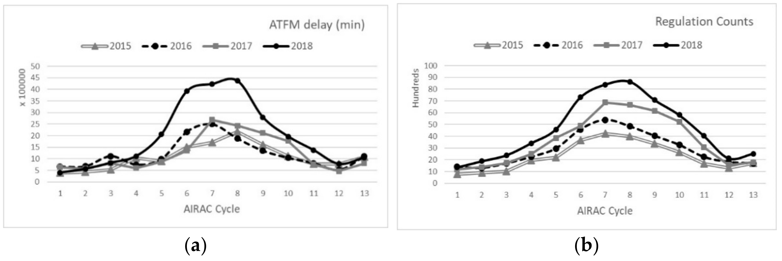
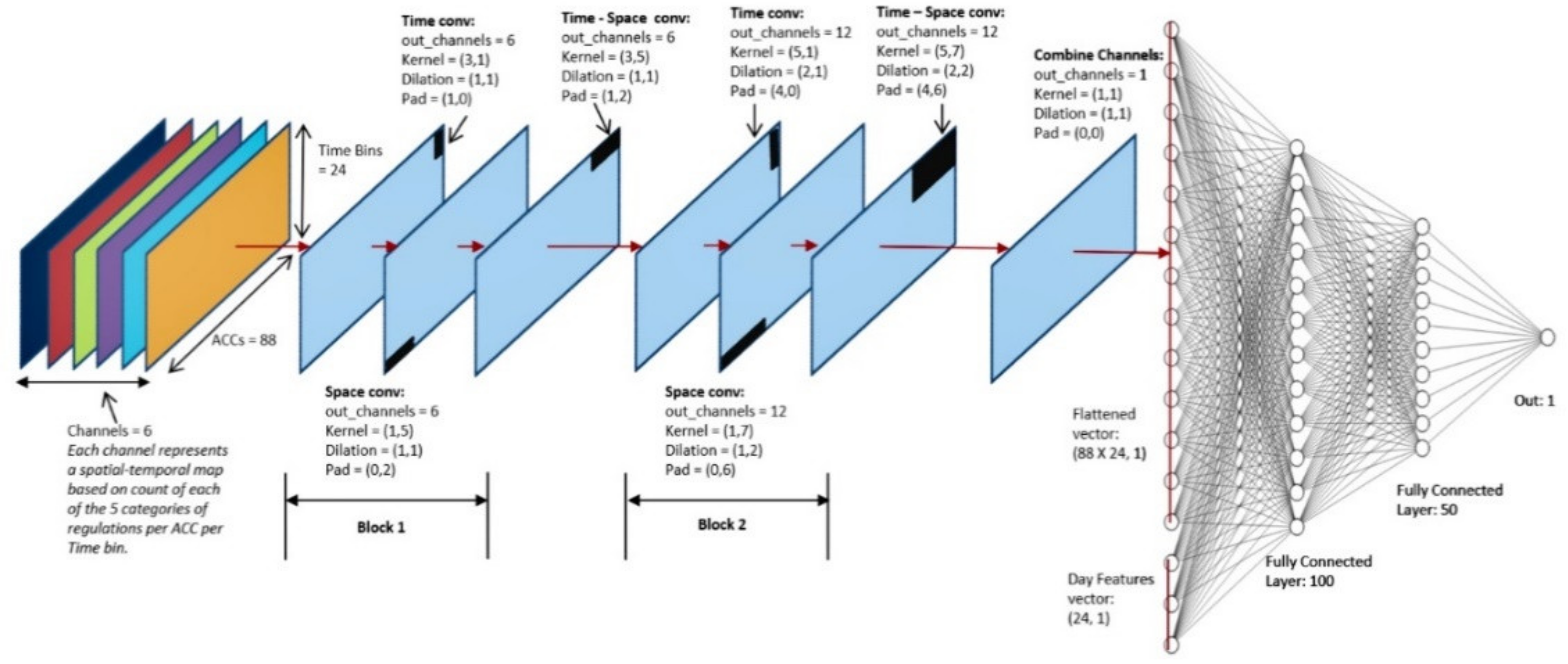
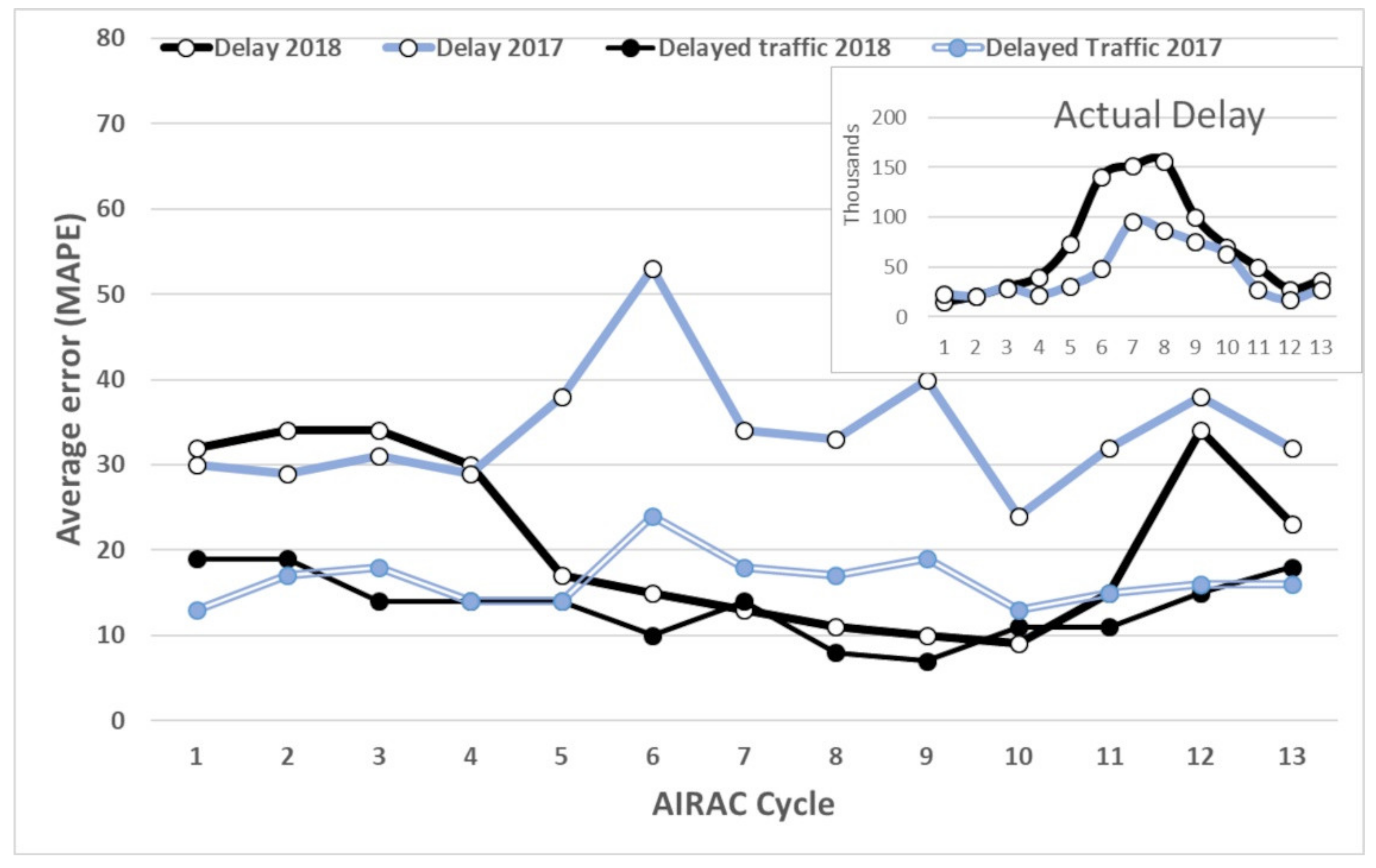
Before parsing the data, we did a general statistical survey on the data from 2015 to 2018. We used aeronautical information regulation and control (AIRAC) cycles. Each cycle is a twenty-eight day period, so a year has 13 cycles. The plans in European airspace are being finalized in different time frames. As provided in Figure 1, different seasonal traffic pattern is also seen in both delay and count of regulations (summer season is from the fifth to tenth cycle). In general, ATFM delay and number of regulations are proportional to each other. However, an increase in the number of regulations is not necessarily followed by an increase in total delay in each cycle. For example, the delay in the sixth cycle of 2017 was less than the delay in the year 2016 for the same AIRAC, even though the number of regulations were more in 2017 compared to 2016. Another observation is the delay jump in 2018, which is regarded as an important sign of reaching a saturated network.

2.1.3. Data Preparation

From the initial survey, we got a better picture on choosing the right data range. The annual growth of delay, regulation counts, and persistent seasonal patterns suggest the use of most recent years. This trend is stronger in 2018 with the highest number of regulations and the highest amount of delay. In essence, supervised learning methods are set for generalization of the learned characteristics to the whole data. Therefore, we combined both the 2018 and 2017 list of regulations to not only support the generalization but also to provide more data points for train and test sets.
Daywise Features and Target Values
Let dop represent the day of operation and N be the number of such days in the post-operational regulations data from NMIR. The goal of our study is to predict the target values at the end of the day based on a set of pre-tactical regulations. This approach conceptually encapsulates all the dynamics of the tactical phase (dop) as a black box for learning algorithm. Accordingly, each day is filtered for regulations activated before 6:00 UTC to obtain a set of features. The data is filtered by regulation activation date (Table 1) for each dop. With this filtering, a new dataset is obtained, from which the daily aggregated features are formed with specified weekday and respective AIRAC cycle. This combination forms the feature vector for each dop.
As explained, both ANM messages and NMIR provide regulation data. We take the similar features in both so that the final learning architecture can eventually take ANM messages as input vector for prediction at tactical phase (NMIR provides postoperational data). Therefore, the following aggregated features are obtained from NMIR data:
  • CountRegPub: Regulation count for each dop, which are activated from the pre-tactical phase up until 6:00 UTC in the tactical phase.
  • AvgRegDurPub: Average duration of all the regulations for each dop, which are activated from the pre-tactical phase up until 6:00 UTC in the tactical phase.
  • DopActivationCounts: Number of regulations activated in the tactical phase of operation, that is from 0:00 UTC up until 6:00 UTC for each dop.
  • CountNumACCPub: Number of ACCs that have activated regulations for each dop from the pre-tactical phase up until 6:00 UTC in the tactical phase.
  • RegulationTypes: Type-related regulation count activated up until 6:00 UTC for each dop. There are total of 14 regulation types (Table A2), and hence 14 features are obtained.
  • AIRAC: The AIRAC cycle (1 to 13) to which each dop belongs. This feature is not available in the postoperational regulations data from NMIR and is added from a database, which can be found in (Table A3). In the context of ML, the AIRAC cycle should be considered as categorical data. This is because AIRAC13 is not greater than AIRAC1, or vice versa in any sense. Therefore, this feature has to be encoded such that learning model can use it without giving numerical significance to the AIRAC number. The one-hot-encoding of Scikit-learn [23] preprocessing module is used for this purpose. With such an encoding, any AIRAC is represented by a binary vector of length 13 and only one of the items in the vector will have a binary high.
  • Weekday: The weekday of each dop. Sun et al. [24] showed that there is weekday variation in the European air transportation network connectivity. Consequently, the weekday is also considered as a feature for the models. Like AIRAC, the seven weekdays are one-hot-encoded, resulting in a binary vector of length 7.
Daywise Target Values
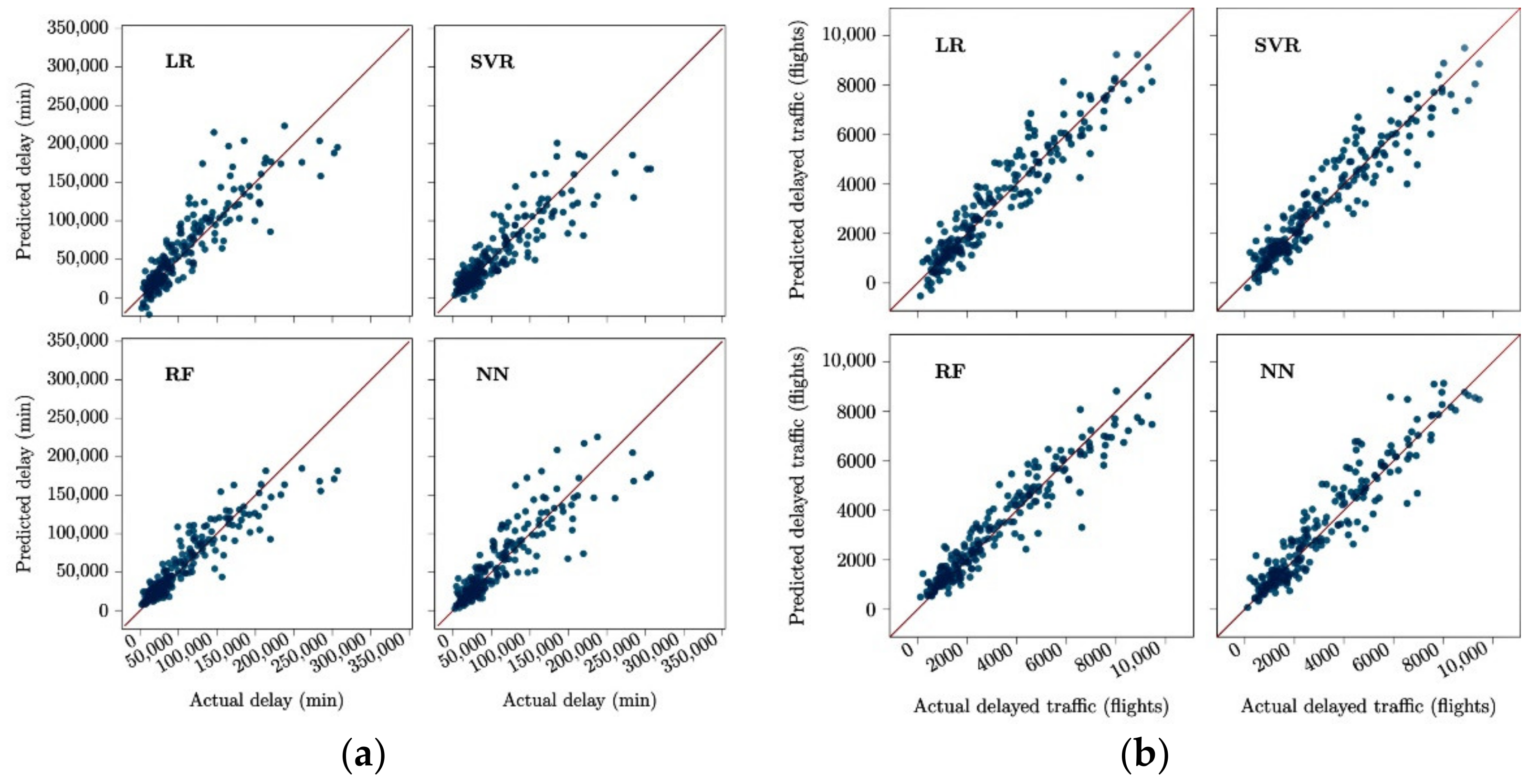
The total daily ATFM delay and most penalized (MP) delayed traffic (hereafter delay and delayed traffic) are considered as the target values (labels) to be predicted by supervised learning model. These values contribute to understanding the level of disruption in the whole network in terms of volume (delay) and extent (count of delayed flights). More specifically target values are:
  • Delay (min): The total daily ATFM delay in the network (24:00 UTC) for each dop.
  • Delayed Traffic (flights): The daily MP delayed traffic (24:00 UTC) for each dop. Note that a flight can be subject to more than one regulation. In such cases, only the most penalizing regulation is considered (to impose a delay), and other regulations are ignored for the flight.
Train-Test Split
With the procedure explained previously, a daily dataset of 730 days in total is prepared from NMIR data on 2017 and 2018. There are two important considerations that have to be made during the train-test split of this data.
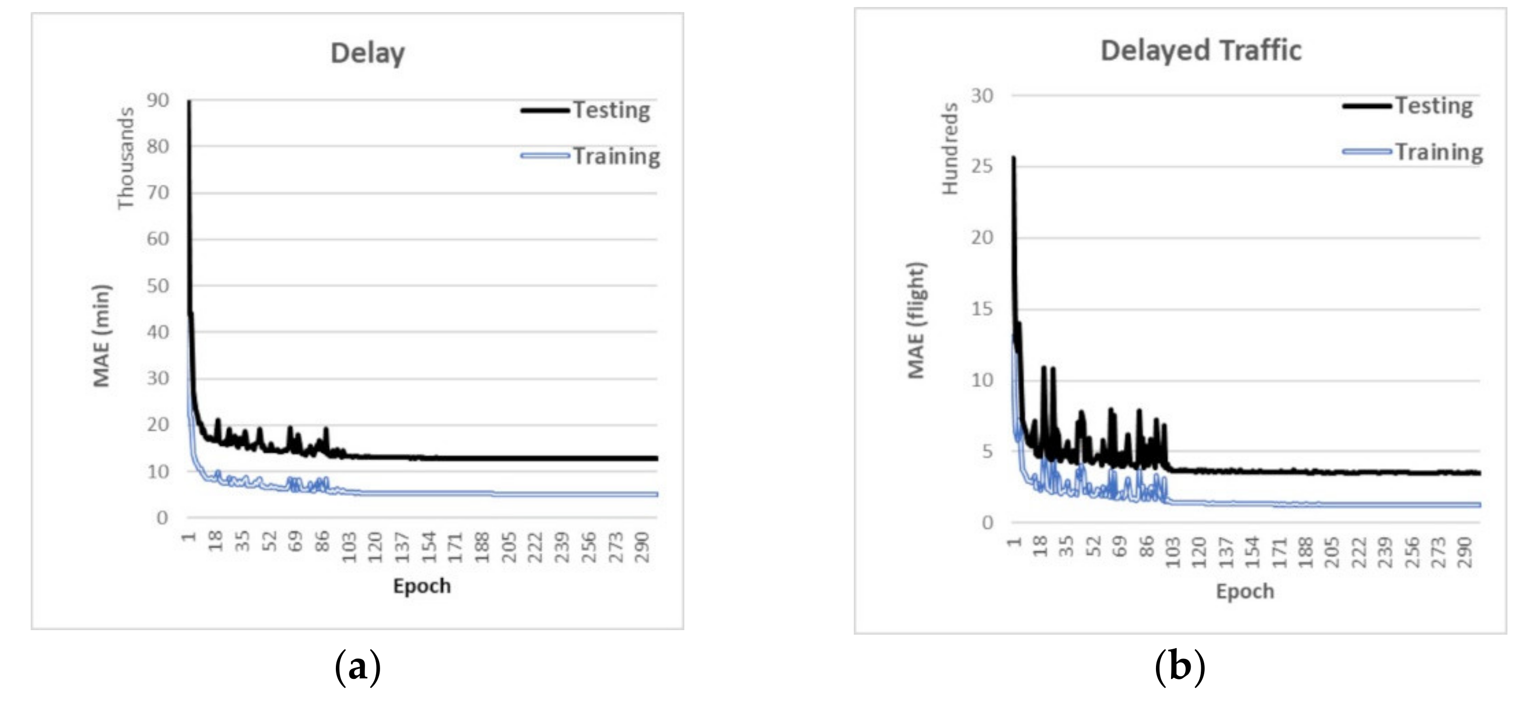
The train-test split ratio in learning models is important, since a relatively larger training set compared to the testing set would increase the risk of overfitting and a smaller training set would challenge the generalization ability of the model. By considering the size of our dataset, we use 70% of the data for training and 30% for testing to address the above issues. Such a choice is not critical in this study because the seasonal trend in the data is evident and this relaxes the use of relatively smaller training set compared to a situation that data dispersion is not showing any meaningful trends.
Stratified Split
The method for splitting the data is also chosen in order to further consider the seasonal trend in regulation data. This is about how we select 70% of the data to form the training set and leaving the rest for test set. Instead of random splitting, the stratified split method is used. A random selection does not assure proper sampling that represents variations in the whole data. Therefore, we ruled out a random selection to maintain model generalization ability.
Stratified train-test split is a splitting method from the Scikit-learn library [23]. It ensures that the variability in the training set is represented in the testing set and hence reduces the risk of underfitting in training set and provides homogeneous sets for both. The variability of the dataset means the distribution of the label values. The stratified split can be based on only one of the labels that is either the delay or delayed traffic. Since the delay has a wider range of values (1958 to 327,795 min), it is chosen as the (label) value on which the stratified split is performed.
The input values to the stratified split should be discrete subsets with at least two samples in each subset. Delays are integer values, and in order to make the subsets, daily values are divided by 20,000 and then rounded to upper integer. Also, after division, any value bigger than 10 is rounded to 10. This accounts for few days with high delay values. These steps led to ten discrete subsets as inputs for stratified split along with split ratio.
Feature Scaling
For each regulation there are numerical fields with different ranges (Table 1). Therefore, it is necessary to use feature scaling to control the effect of various ranges. The risk is that the weights in the learning process tend to be affected more by larger values of features. However, not all learning models are exposed to this risk. This is more relevant to distance-based models such as neural networks (NNs). For instance, RF does not require feature scaling, since it is a tree-based model (nonparametric and nonlinear) and is not influenced by magnitude of the features.
Min-max scaling and standardization are the two common ways to perform feature scaling. In min-max scaling, the values of a feature are scaled to positive value smaller or equal to 1. Equation (1) converts each value from set X to a scaled value yi:
y i = x i min X max x min X     .  
Similarly, standardization scales the values using the standard normal distribution. When the features contain outliers, the min-max scaling compresses the values to a small range. On the other hand, standardization is less sensitive to outliers but does not bind the values between 0 and 1. Consequently, we take the MinMaxScaler from Scikit-learn (for support vector regression, linear regression, and NN models) to ensure uniformity and especially to avoid instability in training of NNs. Accordingly, the scaling statistics are computed on the training set only, and the computed parameters are then used to transform the test set.

2.2. Baseline: Supervised Learning Models

ML is an approach that is more suitable to problems with complex nonlinear structures in which data acquisition is much easier than modeling the problem. In addition, compared to deterministic optimization models, ML applications are mainly about generalization. Therefore, prediction and regression problems are the main use cases for learning models. These models have a combination of optimization cores and statistical analysis in their algorithms.
In Europe, the Single European Sky ATM Research (SESAR) initiative is driving an extensive research program in search of inovative solutions for future ATM. According to the SESAR publications, the application of ML has gained more interest since 2017. NNs were used in [25,26] to predict the flight trajectories and flight levels, respectively. In [27], the authors used gradient boost to predict the runway occupancy count in an airport. Gradient boost and recurrent neural network (RNN) are also addressed in predicting take-off times [28]. Among different supervised learning approaches, applications of NNs cover more topics of ATM [29,30].
RF was used to predict the flight efficiency [31]. However, the prediction of daily delay and delayed traffic at network level by ML techniques remains as a gap. The closest work is in [32], where a simple decision tree model was used to find the delay variations in a small group of sectors and not the whole of European airspace.
Since our approch is so far not investigated by ML, we initially started with four different supervised learning methods to guide our modeling approach and set a baseline to assess the efficiency of our proposed DCNN model. These explored methods are RF, linear regression (LR), support vector regression (SVR), and neural network (NN). The comparison between these models requires similar performance metrics.

2.2.1. Performance Metrics

In regression problems, performance metrics like mean absolute error (MAE), root mean squared error (RMSE) and coefficient of determination (R2) are more common. However, the ranges of target values in regulation data require a customized metric. The wide range of predicted delay covers a minimum of 1958 and a maximum of 327,795 min. Similarly, delayed traffic can be as small as 117 flights and reach 10,812 flights. These metrics treat the deviations equally, but this ignores the operational understanding of data. For example, a deviation of 50,000 min is not acceptable for an actual target value of 50,000 min, but is considered as a decent error when the target value is 350,000 min. Therefore, it is risky to rely on such metrics to evaluate the overall performance of the model. We answered this aspect by the following two solutions.
• Mean absolute percentage error (MAPE)
Similar to MAE, this metric is the average value of errors that is expressed in percentages. Suppose yi is the actual value for which the prediction is ŷi, then the MAPE is given by Equation (2):
M A P E = 100   N N y i ŷ i ŷ i   .  
• Evaluation per delay category
Based on the delay statistics in 2017 and 2018, the delays can be categorized into three categories: low (less than the 25th percentile), moderate (from the 25th to the 75th percentile), and high (greater than the 75th percentile) as given in Table 2. Evaluating the performance at these categories for both delay and delayed traffic provides a better insight into quality of predictions.

2.2.2. Baseline Models

Our approach to predict network disruptions in terms of severity (delay) and dispersion (delayed traffic), as mentioned, has two main contributions: data (regulations) and methodology (i.e., ML). Therefore, it is essential to establish a baseline. Four ML models are explored consequently. LR, SVR, RF and a NN architecture are initially trained and evaluated independently. Then tuned models are compared on their performance on the test set to choose the baseline model (i.e., RF).
The general loss functions of ML models are subject to optimization challenges if the model is set to predict two variables (delay and delayed traffic) simultaneously. This is due to the fact that the optimization function takes the result of the loss function for the learning process (minimizing the error by back propagation). Therefore, if not tailored properly, the measured error of multivariate prediction misleads the optimization model in favor of one of the predicted values.
Since the delay and MP regulated flights are from different scales, we considered three options to face the optimization challenge. These options are either scaling the predicted values, using the weighted loss function, or predicting by separate models for each variable. Because the purpose of this phase of our study was to find a baseline, and the computation time was not the main goal of our study, we proceeded with using separate models for prediction.

Linear Regression (LR)

As one of the basic prediction models, LR is a method to estimate a linear function of independent variables. If γ is the response variable that is assumed to be dependent on a set of predictor variables (X), then it can be approximated by using a linear model as of Equation (3):
Y = α 0 + α 1 X + ε   ,    
where α0 and α1 are constants called the model regression coefficients or weights, and ε is a random disturbance or error. The gradient descent optimization technique is usually used to find the optimal coefficients that minimizes the error.
It is intuitive that the relation between features of regulations and the target values are less likely to be linear, but, apart from linearity assumption, LR considers ε as an independent random quantity with standard normal distribution [33]. Therefore, using the Scikit-learn library, we used LR to check a model with mentioned assumptions.
The data were prepared, scaled and split as explained in Section 2.1. The LR model was trained using the training set of 511 days. The performance metrics of this model on training and testing set are shown in Table 3 and Table A6 for delay and delayed traffic predictions, respectively.
Table 3 provides different performance metrics to show the performance of the LR. A quick look on the metrics shows that poor performance of LR is not convenient enough to consider a linear relationship between independent and response variables. In addition, the MAPE metric shows its advantage over other metrics: even when categories are ignored (overall), it still shows the low quality of predictions, while metrics such as R2 indicate a relatively good prediction (e.g., 0.82 in training). Moreover, MAE takes smaller values in the low category unlike MAPE. This is due to the fact that absolute error function is used to fit the model, meaning that the cost function is evenly penalizing deviations in different ranges of target values. This leads to smaller MAE for the low category, which get worse by higher ranges of delay. The same pattern is seen for delayed traffic in Table A6.

Support Vector Regression (SVR)

Next, we tried SVR to evaluate the nonlinearity. SVR is a derivative of support vector machines (SVMs) that are more efficient in classification problems. SVRs are known to perform well on small and medium-size datasets, but, unlike LR, there are hyper parameters that can to be tuned.
Generally, SVR tries to find a function (hyperplane) that is surrounded by an error tube. This tube reformulates the optimization problem to find the flattest tube that best approximates the hyperplane, which contains most of the training instances (refer to chapter 4 of [34]).
SVR’s hyperparameters are kernel, C, epsilon, and gamma, which are briefly described below:
  • Epsilon: Defines the size of the tube in which no penalty is considered in the training loss function. Higher epsilon values improve generalization and lead to a more relaxed model to be fit on the data.
  • C: The regularization parameter that defines the extent to which the outliers are to be penalized while fitting the model. A large penalization on outliers may result in the model overfitting the data and results in poor generalization.
  • Kernel: In case of a nonlinear relation between independent variables (features) and the response variable a transformation function (a kernel) is used instead of a hyperplane. A kernel can be either linear, polynomial or a radial basis function (RBF), which is an exponential function.
  • Gamma: The kernel coefficient when the kernel is either a RBF or polynomial function. It is a positive value that defines the influence of each training sample. Higher values of gamma lead to a more complex kernel increasing the chances of over-fitting.
Since SVR needs to be tuned (in Scikit-learn library), we performed a grid search over different combinations of hyperparameters in the training set for both delay and delayed traffic:
  • Epsilon: 0.1, 0.5, 1.5, 2, 2.5
  • C: 1, 100, 5000, 80,000 and 10,000
  • Kernel: “Linear”, “Poly” and “RBF”
  • Gamma: 0.01, 0.1, 1, “auto”
The grid search leads to selection of different values for delay and delayed traffic. The significance of nonlinearity for delay is once more identified by the selection of a polynomial kernel as the best kernel (Table 4).
Performance metrics of tuned SVR model show a similar pattern to that observed by LR model. For instance, degradation of prediction quality over the low category is repeated (Table 5 and Table A7). In general, SVR shows better performance compared to LR. However, the model seems to be overfitted for delay compared to consistent prediction for delayed traffic. The assigned values for hyperparameters explain such an overfitted model. The use of a polynomial kernel, larger gamma value and lower regularization parameter (C) leads to a complex learning model that highly fits on the training set.
Despite better performance of SVR for delayed traffic (Table A7: the MAPE metric is 26.46% for the overall category in the test set), it is required to search for other learning models because our purpose is to find one approach that provides acceptable performance for both delay and delayed traffic.

Random Forest Regression (RF)

RF is a typical example of ensemble learning methods that employ multiple learners (weak learners) to generate a weighted prediction (strong learner) as the final result. Ensemble learning is known to provide better generalization ability and more accurate prediction [34].
Generally, an RF model can fit perfectly on the training set by either unlimited depth, or unconstrained minimum samples for each split. However, without tuning the hyperparameters the performance on the test set is expected to be unsatisfactory. The important hyperparameters and their significance are explained below:
  • Number of trees: Defines the number of estimators in a forest. More estimators contribute to better generalization.
  • Maximum depth: Controls to what extent the splitting should be considered at each tree. Smaller depth avoids chances of overfitting.
  • Maximum features: It is the maximum number of features that are considered in splitting process. Selecting only a subset of features for building a regression tree minimizes the over fitting risk.
  • Bootstrap: This is a powerful statistical method for estimating a quantity from a data sample. RF is a bootstrap aggregation (bagging) algorithm. Activated bootstrap allows creating random subsamples of the main dataset with replacement (same value can be used multiple times). In Scikit-learn library, this is a Boolean variable for which, if set to false, the whole dataset is used to build each tree without resampling.
Since RF aggregates the output from a number of weak estimators, the type of features are not as sensitive as previous models. In our case, categorical features such as AIRAC cycle and weekday are not required to be encoded. We performed a grid search to find the best combination of the hyperparameters from the following ranges:
  • Number of trees: 50, 70, 100, 130
  • max_features: 2, 4, 6, 8, 10
  • max_depth: 5, 10, 20, 25, 50
  • bootstrap: True, False.
RF tends to overfit by higher values of max_depth (Table A4 and Table A5). Therefore, the grid search selects 50 on the training set (Table 6). However, we tested lower values of this parameter and concluded that a value of 12 avoids overfitting and any value below 12 leads to underfitting.
The performance of RF with max_depth of 12 on training and testing set is provided in Table 7 and Table A8 for delay and delayed traffic predictions, respectively. The performance of RF on the test set is measured to be better than SVR and LR. In addition, the same approach of choosing the hyperparameters provides a tuned model for both delay and delayed traffic.
RF proved to provide best performance as a baseline because of its tree-based approach and tuned hyperparameters. However, another major approach in regression problems is NNs, which recently has been applied on regulation data. In [35], the authors proposed a NN that outperforms a RF model in predicting delay, therefore we also tested a NN.

Neural Networks (NNs)

These networks learn in a hierarchical order and their structure involves multiple levels of abstraction for knowledge representation. NNs accumulate propagated information through higher levels in a sequential order such that learning at each layer is based on statistical learning procedures at the previous layers (refer to chapter 7 of [34]).
In general, NNs basically deal with the nonlinearity by the activation function. A network can have different activation functions at each layer. Furthermore, prediction errors are evaluated by cost (loss) function and through iterations, optimization function pushes the network toward minimizing the errors. Each iteration is performed on batches that are subsets of the training set. The calculations on a batch is finalized by updating the weights of the nodes at each layer. An epoch is completed when all the batches of a training set are fed as inputs.
We used Keras [36] to implement the NN architecture. A fully connected sequential NN with three hidden layers is used. The input layer has 38 neurons, corresponding to the length of the feature vector. The three hidden layers converge from 100 to 50, and 25 neurons. A single neuron at the output predicts the delay or the delayed traffic for the two separate models, respectively. Each layer uses rectified linear unit (ReLU) as the activation function. The model is trained with MAE cost function and Adam optimizer for 500 epochs with a batch size of 30.
Considering the model performance in Table 8 and Table A8, the tested architecture is not considered to be overfitted, since the metrics report similar quality of prediction for training and testing sets.
We have considered four different approaches for regression problem and the performance of each model is measured with both standard metrics (R2 and MAE) and customized metric of MAPE (Table 9). All models had challenges in predicting lower category and precision improves for bigger values. Models that are designed to cope with nonlinearity such as NN outperform linear models (LR). Furthermore, the dispersion of predictions is visualized (Figure 2) to guide the selection of baseline model. The optimization of RF hyperparameters not only led to higher precision but also the scatter plot shows a steady narrow prediction error for both delay and delayed traffic.
Up to this stage, the results show that RF and NN deliver higher quality of prediction in our study. Since NNs are more flexible than RF, we select RF as the baseline model and focus on a NN based architecture to improve the predictions.

2.3. Proposed Deep Convolutional Neural Network (DCNN)

In the previous section, we describe our preprocessing on data and aggregation of data features for selection of baseline model. The aggregation of data ignores the spatiotemporal features to a great extent. Yet, the traffic flows connect separate area control centers (ACC) across Europe and regulated traffic volumes may lead to secondary effects on other traffic volumes. The propagation of this consequential impact is known as network effect in ATFCM [32]. Such secondary effects can be perceived better by CNNs that are designed to capture different features of data through convolutional layers.
CNNs are mainly employed for classification problems, especially in image processing, where learning is about spatial characters. Relatively few studies try to extract spatiotemporal features by CNN. For instance, in intelligent transportation systems, Shen et al. [37] proposed a deep three-dimensional CNN to extract the spatial and temporal correlations. They evaluated the model with a New York taxi trajectory dataset. Furthermore, a recurrent CNN was developed in a study by Wang et al. [38] to predict the traffic speed and congestion. Their model integrated the spatiotemporal traffic speeds of contiguous road segments as the input matrix.
The architecture of such deep networks is identical to each study because deep networks have higher degrees of freedom compared to other learning methods. In fact, apart from hyperparameters of CNN such as kernel size and stride, the model design can also be different in selection of activation functions, optimization methods, etc. We proposed a DCNN that considers the network effect by extracting deep characteristics of regulation data.

2.3.1. Data Preparation

Based on the experience that is obtained from exploring different baseline candidates, the postoperational data needed to be processed differently for the DCNN model. However, the same span of data (2017 and 2018) is considered to allow comparison with the baseline model.
Along with the spatiotemporal map, other daily features representing each day are added to include more features in the model. These are the same features that were used for baseline models except regulation types that are included as channels in DCNN. This results in a feature vector with a length of 24 to represent each day as follows:
  • CountRegPub, AvgRegDurPub, DopActivationCounts, and CountNumACCPub (Section 2.1.3);
  • AIRAC cycles that add 13 encoded features;
  • Weekdays that are converted into seven encoded features.
Spatiotemporal Feature Map
In order to construct the feature map for convolutional layers, it is possible to take either traffic volumes (TVs) or ACCs for spatial bins. However, we took the ACCs since a high number of possible TVs across Europe add to the complexity of the model with no significant benefit. In addition, a division of the data over TVs limits the number of data points for learning, but taking ACCs is a better compromise that avoids detailed granularity while preserving the spatial patterns of regulations in bins. ACCs can be extracted from the TV id (Table 1) for each regulation.
Each day is divided with a bin size of one hour to make the temporal bins. These definitions for spatiotemporal bins build a N × C × H × W matrix that can be taken for a 2D convolution in Pytorch [39]. N corresponds to the number of days, C to the number of channels, H is the time bins and W is the spatial bins. Instead of merging all regulations for each ACC at each time bin, six channels are set as different regulation types as of Table 10.
For the activation function, a variation of ReLU function known as Leaky ReLU is taken, since it supports generalization in deep NNs [40]. Furthermore, the proposed model uses weighted mean absolute error (WMAE) as the cost function to improve predictions for the low category of target values. The weights are calculated from a negative exponential function, Equation (4), which delivers higher magnitude for low target values (yi) and flattens out for medium to large values.
w i = 25 *   y i 1 3     .  

2.3.2. Model Architecture

The proposed model was designed using an iterative process and is inspired by the model in [37]. In their model, the authors have not reasoned why a large number of filters (kernels) were used. Because a large number of filters significantly increases the computational effort, we started with simpler model with few filters and layers. Based on the performance of the model on test set, the filters and the model architecture were iteratively improved to achieve the proposed architecture.
As provided in Figure 3 and Table 11, two blocks of convolution filters are applied to the six input channels (spatiotemporal feature maps). Each block has two independent temporal and spatial filters, which are followed by a spatiotemporal filter to check for correlated patterns. The output of second block (which extracts deeper features) is aggregated with a unit size kernel to get a single channel.
The result of convolutional layers is flattened to a vector and concatenated with daywise feature vector. This vector is processed by a sequential neural network (SNN) with two fully connected layers (100 and 50 neurons). The output of the model is a single neuron that predicts either delay or the delayed traffic.

3. Results

The same training procedure as applied for baseline model is taken for DCNN. The quality of the learning process is given in Figure 4. The impact of altering the loss function to WMAE in both the training and testing phase is equally effective in decreasing the errors. Furthermore, the learning time is significantly shorter than expected (curves are flattened almost after 150 epochs).
In comparison to RF (Table 12) as the baseline model, DCNN delivers an outstanding performance. Predictions for aeronautical information regulation and control (AIRAC) he low category of target values improved the most. MAPE improved 70% for delayed traffic and 60% for delay. The introduced weighting method proved to be efficient in enhancing the model in low category. In general, the proposed architecture successfully improved the results by 50% (overall category).
The ability of DCNN to learn from spatiotemporal features of the regulation also proved to be efficient. Figure 5 provides scatter plots that show prediction precision for both delay and delayed traffic. DCNN outperforms RF (with optimized hyperparameters) and smoothly predicts the target values regardless of their category, while RF scatter plot shows more dispersion as the target values grow.
Apart from the advantages of convolution layers, including SNN in the model’s architecture enables the model to expect disruptive dynamics of tactical phase. Putting more focus on temporal characteristics of regulations by including AIRAC cycles and weekdays in learning can be illustrated better by validation on different data samples.

4. Validation and Discussion

Since the end goal is to contribute to network resiliency, it is essential to observe the performance of proposed model over different data samples. Therefore, we trained the model on postoperational data of two consecutive years to predict the next year. Table 13, summarizes that the model tends to perform better in predicting 2018. However, 2018 is reported as the highest figure of delay in the European aviation. This means more regulations were implemented and more flights were delayed during this year.
Therefore, we investigated the performance of the model in different AIRAC cycles. Figure 6 provides the average daily MAPE values for both delay and delayed traffic predictions. Despite high load of traffic and delay over the summer season (AIRAC 5 to 10), DCNN is more accurate over these periods (error scatter plots are given in Figure A1). The descending pattern of MAPE for all predictions over summer suggests that the number of regulations is a key driver in prediction accuracy. This is expected since our architecture is based on NNs to capture nonlinearity and more regulations means more datapoints from dynamic disruptions. The inverse pattern of prediction accuracy and actual delay (inset in Figure 6) also confirms that DCNN is more affected by number of regulations and perform better in summer. Another observation from Figure 6 is that such an impact (regulation counts) seems to be more than the effect of different ranges of delayed traffic and delay. High number of regulations canceled out the gap between the quality of predictions for delayed traffic and delay in 2018 during summer.
Other factors can also affect the quality of predictions. For instance, relatively high errors in AIRAC 6 2017 predictions based on the data from 2015 and 2016 can be a result of data quality. In fact, the observed errors in prediction of summer 2017 might be an effect of a change in delay calculations, which was implemented from April 2016 onwards [41].
Nevertheless, the enhanced prediction capability of DCNN model compared to RF is clear and seasonal patterns in predictions are consistent with dynamics of EATMN in different AIRAC cycles. The overall errors for a full year prediction are significantly improved. For operational use cases, the prediction is most relevant for a day and not a full year, hence the model is performing well on such a scale.
This study illustrated the benefits of predicting network delay based on regulations. Furthermore, we explored the use of leaning algorithms to deal with the complexity of network predictions. The combination of convolutional layers and a sequential NN in our proposed model proved to be efficient in predicting both delay and delayed traffic. DCNN significantly improved the prediction quality in comparison to an optimized RF model as the baseline model. Our contribution to predict delay based on regulations gives DCNN the advantage to perform better in more dynamic situations, since more regulations provide more data points for the model.
This paper also contributed to the topic of ATM resiliency by providing better networkwide situational awareness. Incidents such as the volcano eruption in 2010 and coronavirus pandemic in 2020 are challenges to different levels of ATM resiliency (Table A1). The volcano eruption was a safety risk in the pre-tactical phase and coronavirus is a large-scale issue in strategic phase. ML approaches depend on sufficient data to learn. The aforementioned cases are exceptions and there is no previous situation that learning models can learn from. Also, in both cases, the system is not suffering from delay but mostly flight cancelation, which is not included in the scope of this work.
The proposed model provides a method to predict delay and delayed traffic at EATMN level based on large-scale capacity measures (regulations). In future studies, the DCNN model can be further improved by including additional features on air traffic demand and airspace capacity. For instance, daily weather forecast can represent a capacity feature and traffic situation (filed flight plans) can add demand figures as model inputs.

Author Contributions

Conceptualization, R.S., B.A.P. and V.G.; methodology, R.S. and B.A.P.; software, B.A.P.; validation, R.S. and B.A.P.; formal analysis, R.S. and B.A.P.; investigation, R.S. and B.A.P.; resources, R.S. and V.G.; data curation, R.S.; writing—original draft preparation, R.S.; writing—review and editing, R.S., B.A.P. and V.G.; visualization, R.S. and B.A.P.; supervision, R.S. and V.G.; project administration, R.S. All authors have read and agreed to the published version of the manuscript.

Funding

This research received no external funding.

Conflicts of Interest

The authors declare no conflict of interest.

Appendix A

Appendix A.1. Resilience Levels

The following table [35] shows the connection of resilience levels with ATFCM phases. Prediction of delay and delayed traffic serves as a key input for different levels of network resiliency (esp. tactical phase).
Table A1. Resilience levels.
LevelFeaturesATFCM
Phase
AbsorptiveRobustness, ReliabilityStrategic *
AdaptiveConsideration of adverse impacts,
Anticipation of disruption,
Recognition of unanticipated events
pre-tactical **
RestorativeControl measures, Conflict handling,
Cost estimation
Tactical ***
Procedural example: * ATFCM Procedural Contingency Plan, ** Reaccommodation of network flows during an ATC strike, *** Flight level capping measures.

Appendix A.2. The Regulation Types

Regulation types are also referred to as regulation causes in related documents such as the ATFCM user manual [20]. Each regulation can be implemented based on a set of provided guidelines for the user to select the right regulation type.
This classification provides more details for delay causes and further support the postoperation analysis. The coding also provides details on regulation location that declares the phase of the delayed flight. In this study, these classes are only used for the learning model without considering the flight phase.
Table A2. Regulation types.
Regulation CodeRegulation Code
C-ATC CapacityE-Aerodrome Services
I-ATC Industrial ActionN-Industrial Action Non-ATC
R-ATC RoutingsM-Airspace Management
S-ATC StaffingP-Special Event
T-ATC EquipmentW-Weather
A-Accident/IncidentV-Environmental Issues
G-Aerodrome CapacityO-Other

Appendix A.3. The AIRAC Cycles from 2015 to 2018

The AIRAC cycles effective dates are obtained from the International Civil Aviation Organization (ICAO) website [42] and compiled as below:
Table A3. Schedule of AIRAC effective dates, 2015–2018.
2015201620172018
08 January07 January05 January04 January
05 February04 February02 February01 February
05 March03 March02 March01 March
02. April31 March30 March29 March
30 April28 April27 April26 April
28 May26 May25 May24 May
25 June23 June22 June21 June
23 July21 July20 July19 July
20 August18 August17 August16 August
17 September15 September14 September13 September
15 October13 October12 October11 October
12 November10 November09 November08 November
10 December08 December07 December06 December

Appendix A.4. Overfitted RF Model

Table A4. Performance of applied RF to predict delay (max_depth = 50).
CategoryTrainTest
DaysMAPE *R2MAE **DaysMAPER2MAE
Low1270.01.005577.04−4.168100
Nominal2610.01.0011127.820.2211208
High1230.01.005318.450.4724829
Overall5110.01.0021937.910.8513724
* in percentage, ** minutes.
Table A5. Performance of applied RF to predict delayed traffic (max_depth = 50).
CategoryTrainTest
DaysMAPE *R2MAE **DaysMAPER2MAE
Low1290.01.005256.20−2.02349
Nominal2560.01.0011317.840.66437
High1260.01.005411.86 0.44765
Overall5110.01.0021925.470.91497
* in percentage, ** flights.

Appendix A.5. DCNN Prediction Performance

Figure A1. Comparative scatter plots for prediction quality of DCNN in different years. (a) Delay, (b) delayed traffic. Model is more precise in predicting lower values.
Aerospace 08 00028 g0a1

Appendix B. Learning Performance (Delayed Traffic)

Table A6. Performance of applied linear regression (LR).
CategoryTrainTest
DaysMAPE *R2MAE **DaysMAPER2MAE
Low12947.98−2.633605264.28−2.07370
Nominal25621. 060.5950311322.000.46569
High12611.420.56727549.90 0.62617
Overall51125.480.9152221929.050.9533
* in percentage, ** flights.
Table A7. Performance of applied SVR.
CategoryTrainTest
DaysMAPE *R2MAE **DaysMAPER2MAE
Low12941.38−1.863085254.79−1.47319
Nominal25618.690.6245711320.760.5536
High12612.820.378355411.100.52697
Overall51122.970.951321926.460.9524
* in percentage, ** flights.
Table A8. Performance of applied RF.
CategoryTrainTest
DaysMAPE *R2MAE **DaysMAPER2MAE
Low1290.01.005255.95−1.96346
Nominal2560.01.0011317.310.68427
High1260.01.005411.640.46749
Overall5110.01.0021925.090.91487
* in percentage, ** flights.
Table A9. Performance of applied NN.
CategoryTrainTest
DaysMAPE *R2MAE **DaysMAPER2MAE
Low12931.02−0.82295247.95−1.46286
Nominal25616.130.6841111323.130.41599
High12611.120.56696549.750.55608
Overall51118.650.9243521925.730.89527
* in percentage, ** flights.

References

  1. European Union. Regulation (EC) No 552/2004 of the European Parliament and of the Council. Off. J. Eur. Union 2004, L 96, 26–42. [Google Scholar]
  2. Kistan, T.; Gardi, A.; Sabatini, R.; Ramasamy, S.; Batuwangala, E. An evolutionary outlook of air traffic flow management techniques. Prog. Aerosp. Sci. 2017, 88, 15–42. [Google Scholar] [CrossRef]
  3. Francis, R.; Bekara, B. A metric and frameworks for resilience analysis of engineered and infrastructure systems. Reliab. Eng. Syst. Saf. 2014, 121, 90–103. [Google Scholar] [CrossRef]
  4. Ivanov, N.; Netjasov, F.; Jovanović, R.; Starita, S.; Strauss, A. Air Traffic Flow Management slot allocation to minimize propagated delay and improve airport slot adherence. Transp. Res. Part A Policy Pract. 2017, 95, 183–197. [Google Scholar] [CrossRef]
  5. Montlaur, A.; Delgado, L. Flight and passenger efficiency-fairness trade-off for ATFM delay assignment. J. Air Transp. Manag. 2020, 83, 101758. [Google Scholar] [CrossRef]
  6. Bolić, T.; Castelli, L.; Corolli, L.; Rigonat, D. Reducing ATFM delays through strategic flight planning. Transp. Res. Part E Logist. Transp. Rev. 2017, 98, 42–59. [Google Scholar] [CrossRef] [Green Version]
  7. Chang, Y.-H.; Solak, S.; Clarke, J.-P.B.; Johnson, E.L. Models for single-sector stochastic air traffic flow management under reduced airspace capacity. J. Oper. Res. Soc. 2016, 67, 54–67. [Google Scholar] [CrossRef]
  8. Delgado, L.; Prats, X. En Route Speed Reduction Concept for Absorbing Air Traffic Flow Management Delays. J. Aircr. 2012, 49, 214–224. [Google Scholar] [CrossRef]
  9. Prats, X.; Hansen, M. Green delay programs, absorbing ATFM delay by flying at minimum fuel speed. In Proceedings of the Ninth USA/Europe Air Traffic Management Research and Development Seminar (ATM2011), Berlin, Germany, 14–17 June 2011. [Google Scholar]
  10. Carlier, S.; de Lépinay, I.; Hustache, J.-C.; Jelinek, F. Environmental Impact of Air Traffic Flow Management Delays. In Proceedings of the 7th USA/Europe Air Traffic Management Research and Development Seminar (ATM2007), Seminar, Barcelona, 2–5 July 2007. [Google Scholar]
  11. FAA & EUROCONTROL. 2017 Comparison of Traffic Management-Related Operational Performance U.S./Europe; EUROCONTROL Performance Review Unit and FAA-ATO: Brussels, Belgium, 2019. [Google Scholar]
  12. Bardach, M.; Gringinger, E.; Schrefl, M.; Schuetz, C.G. Predicting Flight Delay Risk Using a Random Forest Classifier Based on Air Traffic Scenarios and Environmental Conditions. In Proceedings of the 2020 AIAA/IEEE 39th Digital Avionics Systems Conference (DASC), San Antonio, TX, USA, 11–16 October 2020. [Google Scholar]
  13. Guo, Z.; Mei, G.; Liu, S.; Pan, L.; Bian, L.; Tang, H.; Wang, D. SGDAN—A Spatio-Temporal Graph Dual-Attention Neural Network for Quantified Flight Delay Prediction. Sensors 2020, 20, 6433. [Google Scholar] [CrossRef] [PubMed]
  14. Zanin, M.; Zhu, Y.; Yan, R.; Dong, P.; Sun, X.; Wandelt, S. Characterization and Prediction of Air Transport Delays in China. Appl. Sci. 2020, 10, 6165. [Google Scholar] [CrossRef]
  15. Gui, G.; Liu, F.; Sun, J.; Yang, J.; Zhou, Z.; Zhao, D. Flight delay prediction based on aviation big data and machine learning. IEEE Trans. Veh. Technol. 2019, 69, 140–150. [Google Scholar] [CrossRef]
  16. Gui, G.; Zhou, Z.; Wang, J.; Liu, F.; Sun, J. Machine Learning Aided Air Traffic Flow Analysis Based on on Aviation Big Data. IEEE Trans. Veh. Technol. 2020, 69, 4817–4826. [Google Scholar] [CrossRef]
  17. Melgosa, M.; Prats, X.; Xu, Y.; Delgado, L. Enhanced Demand and Capacity Balancing based on Alternative Trajectory Options and Traffic Volume Hotspot Detection. In Proceedings of the 2019 IEEE/AIAA 38th Digital Avionics Systems Conference (DASC), San Diego, CA, USA, 8–12 September 2019. [Google Scholar]
  18. Xu, Y.; Prats, X.; Delahaye, D. Synchronised demand-capacity balancing in collaborative air traffic flow management. Transp. Res. Part C Emerg. Technol. 2020, 114, 359–376. [Google Scholar] [CrossRef] [Green Version]
  19. Bertsimas, D.; Lulli, G.; Odoni, A. An Integer Optimization Approach to Large-Scale Air Traffic Flow Management. Oper. Res. 2011, 59, 211–227. [Google Scholar] [CrossRef]
  20. Niarchakou, M.C.S. ATFCM Operations Manual, 23.1 ed.; EUROCONTROL: Brussels, Belgium, 2019. [Google Scholar]
  21. EUROCONTROL. NOP (Network Operations Portal). 2020. Available online: https://www.public.nm.eurocontrol.int/PUBPORTAL/ (accessed on 17 February 2020).
  22. EUROCONTROL. NMIR (Network Manager Interactive Reporting). 2020. Available online: https://www.eurocontrol.int/dashboard/network-manager-interactive-reporting-dashboard (accessed on 24 September 2019).
  23. Pedregosa, F.; Varoquaux, G.; Gramfort, A.; Michel, V.; Thirion, B.; Grisel, O.; Blondel, M.; Prettenhofer, P.; Weiss, R.; Dubourg, V.; et al. Scikit-learn: Machine learning in Python. J. Mach. Learn. Res. 2011, 12, 2825–2830. [Google Scholar]
  24. Sun, X.; Wandelt, S.; Linke, F. Temporal evolution analysis of the European air transportation system: Air navigation route network and airport network. Transp. B Transp. Dyn. 2014, 3, 153–168. [Google Scholar] [CrossRef]
  25. Wang, Z.; Liang, M.; Delahaye, D. Short-term 4D Trajectory Prediction Using Machine Learning Methods. In Proceedings of the Seventh SESAR Innovation Days, Belgrade, Serbia, 28–30 November 2017. [Google Scholar]
  26. Poppe, M.; Scharff, R.; Buxbaum, J.; Fieberg, D. Flight Level Prediction with a Deep Feedforward Network. In Proceedings of the Eighth SESAR Innovation Days, Salzburg, Austria, 3–7 December 2018. [Google Scholar]
  27. Martinez, D.; Belkoura, S.; Cristobal, S.; Herrema, F.; Wachter, P. A Boosted Tree Framework for Runway Occupancy and Exit. In Proceedings of the Eighth SESAR Innovation Days, Salzburg, Austria, 3–7 December 2018. [Google Scholar]
  28. Dalmau, R.; Ballerini, F.; Naessens, H.; Belkoura, S.; Wangnick, S. Improving the Predictability of Take-off Times with Machine Learning. In Proceedings of the Ninth SESAR Innovation Days, Athens, Greece, 2–5 December 2019. [Google Scholar]
  29. Mori, R.; Delahaye, D. Simulation-Free Runway Balancing Optimization under Uncertainty Using Neural Network. In Proceedings of the Ninth SESAR Innovation Days, Athens, Greece, 2–5 December 2019. [Google Scholar]
  30. Fernandez, A.; Martınez, D.; Hernandez, P.; Cristobal, S.; Schwaiger, F.; Nunez, J.M. Flight Data Monitoring (FDM) Unknown Hazards detection during Approach Phase using Clustering Techniques and AutoEncoders. In Proceedings of the Ninth SESAR Innovation Days, Athens, Greece, 2–5 December 2019. [Google Scholar]
  31. Marcos, R.; Herranz, R.; Vázquez, R.R.; García-Albertos, P.; Cantú Ros, O.G. Application of Machine Learning for ATM Performance Assessment–Identification of Sources of En-Route Flight Inefficiency. In Proceedings of the Eighth SESAR Innovation Days, Salzburg, Austria, 3–7 December 2018. [Google Scholar]
  32. Le Foll, B.P. Network Effect: A Possible Model to Highlight Interdependencies between Flow Management Regulations. Master’s Thesis, Faculty of Transport and Traffic Engineering of Belgrade, Belgrade, Serbia, 2005. [Google Scholar]
  33. Chatterjee, S.; Hadi, A.S.H. Regression Analysis by Example, 5th ed.; John Wiley & Sons: Hoboken, NJ, USA, 2015. [Google Scholar]
  34. Awad, M.; Khanna, R. Efficient Learning Machines, 1st ed.; Apress: New York, NY, USA, 2015. [Google Scholar]
  35. Sanaei, R.; Lau, A.; Linke, F.; Gollnick, V. Machine Learning Application in Network Resiliency based on Capacity Regulations. In Proceedings of the 2019 IEEE/AIAA 38th Digital Avionics Systems Conference (DASC), San Diego, CA, USA, 8–12 September 2019. [Google Scholar]
  36. Chollet, F. Keras: Deep Learning Library for Theano and Tensorflow. 2015. Available online: https://keras.io (accessed on 17 October 2019).
  37. Shen, B.; Liang, X.; Ouyang, Y.; Liu, M.; Zheng, W.; Carley, K. Stepdeep: A novel spatial-temporal mobility event prediction framework based on deep neural network. In Proceedings of the 24th ACM SIGKDD International Conference on Knowledge Discovery & Data Mining, London, UK, 19–23 August 2018. [Google Scholar]
  38. Wang, J.; Gu, Q.; Wu, J.; Liu, G.; Xiong, Z. Traffic Speed Prediction and Congestion Source Exploration: A Deep Learning Method. In Proceedings of the 2016 IEEE 16th International Conference on Data Mining (ICDM), Barcelona, Spain, 12–15 December 2016. [Google Scholar]
  39. Paszke, A.; Gross, S.; Chintala, S.; Chanan, G.; Yang, E.; DeVito, Z.; Lin, Z.; Desmaison, A.; Antiga, L.; Lerer, A. Automatic differentiation in PyTorch. In Proceedings of the NIPS 2017 Autodiff Workshop, Long Beach, CA, USA, 9 December 2017. [Google Scholar]
  40. Maas, A.L.; Hannun, A.Y.; Ng, A.Y. Rectifier nonlinearities improve neural network acoustic models. In Proceedings of the International Conference on Machine Learning (ICML), Atlanta, Greece, 16–21 June 2013. [Google Scholar]
  41. EUROCONTROL. NM Release Presentation to Externals; EUROCONTROL: Brussels, Belgium, 2016. [Google Scholar]
  42. ICAO; AIRAC. International Civil Aviation Organization. Available online: https://www.icao.int/Safety/information-management/Pages/AIRACAdherence.aspx (accessed on 20 September 2020).
Figure 1. Statistical survey of regulation data per aeronautical information regulation and control (AIRAC) cycle to compare (a) total air traffic flow management (ATFM) delay and (b) regulation count. Apart from seasonal patterns, this figure shows that an increase in number of regulations does not necessarily mean an increase in the ATFM delay.
Aerospace 08 00028 g001
Figure 2. Scatter plots for prediction quality of learning models on test set. (a) Delay, (b) delayed traffic. Explored models perform better on delayed traffic due to its smaller range compared to delay. RF (random forest) provides minimum errors with symmetrical low dispersion.
Aerospace 08 00028 g002
Figure 3. Proposed architecture for deep convolutional neural network (DCNN). Channels are set based on the regulation types and two blocks of convolutional layers, which learn the spatiotemporal characters of regulations.
Aerospace 08 00028 g003
Figure 4. Learning curve of DCNN through training and testing phase. (a) Delay, (b) delayed traffic. Use of weighted mean absolute error (WMAE) improved learning time.
Aerospace 08 00028 g004
Figure 5. Comparative scatter plots of prediction quality. Plots on top are from DCNN and the bottom plots are from baseline model (i.e., random forest): (a) delay, (b) delayed traffic.
Aerospace 08 00028 g005
Figure 6. DCNN validation: prediction errors in different AIRAC cycles. More regulations in 2018 (especially during summer season) provide better prediction quality regardless of the expected high values for both delay and delayed traffic.
Aerospace 08 00028 g006
Table 1. Regulation’s data set structure (network manager interactive reporting; NMIR).
FieldSample EntryFieldSample Entry
TVS IdEDYYFMPReg Activation Notice *98
Reg IdYBWST01Reg Duration *42
Protected Location IdEDYYBWSTReg Reason NameS-ATC Staffing
Protected Location TypeAirspaceReg Window Width *10
TV Id MASBWSTMP Regulated Traffic **90
Reg Start Time01.01.2018 20:00:00Regulated Traffic **93
Reg Truncated Start Time01.01.2018ATFM Delay *259
Reg End Date01.01.2018 21:40:00MP Delayed Traffic **24
Reg Cancel StatusCancelledAvg Delay per Regulated Traffic * 2.8
Reg Cancel Date01.01.2018 20:42:21Reg Description(text)
Reg Activation Date01.01.2018 18:22:19Day of the WeekMonday
* in minutes, ** flight count.
Table 2. Categorization ranges for model performance evaluation.
CategoryDelay
(min)
Delayed Traffic (Flights)
Low[0, 20,000)[0, 1250)
Moderate[20,000, 80,000][1250, 4650]
High(80,000, ∞)(4650, ∞)
Table 3. Performance of applied LR to predict delay.
CategoryTrainTest
DaysMAPE *R2MAE **DaysMAPER2MAE
Low12777.59−5.8187445592.51−5.548562
Nominal26134.85−0.1413,75311136.1−0.3314,834
High12318.020.5624,3295322.530.2627,884
Overall51141.470.8215,05421946.980.7716,417
* in percentage, ** minutes.
Table 4. Best hyper-parameters for support vector regression (SVR).
Response ValueEpsilonCKernelGamma
Delay2.55000Poly1
Delayed traffic210,000Linear0.1
Table 5. Performance of applied SVR to predict delay.
CategoryTrainTest
DaysMAPE *R2MAE **DaysMAPER2MAE
Low12730.87‒0.0625535571.64‒4.07361
Nominal26111.310.7475911129.870.1312,068
High12312.420.5718,1155323.410.1731,753
Overall51116.440.88742621938.80.7815,649
* in percentage, ** minutes.
Table 6. Best hyperparameters for RF.
Response ValueNumber of Treesmax_Featuresmax_DepthBootstrap
Delay70650False
Delayed traffic70850False
Table 7. Performance of applied RF to predict delay.
CategoryTrainTest
DaysMAPE *R2MAE **DaysMAPER2MAE
Low1276.760.957465574.15−3.497741
Nominal2611.961.077611126.20.2410,612
High1230.681.07925317.650.4724,263
Overall5112.851.077221936.180.8513,195
* in percentage, ** minutes.
Table 8. Performance of applied NN to predict delay.
CategoryTrainTest
DaysMAPE *R2MAE **DaysMAPER2MAE
Low12754.96−2.5256215559.58−2.985417
Nominal26125.330.2610,68711130.330.0812,334
High12321.010.3628,6935323.940.1830,975
Overall51131.650.8113,76221936.130.7915,108
* in percentage, ** minutes.
Table 9. Performance of explored learning models over test set.
CategoryDelay *Delayed Traffic *
LRSVRRFNNLRSVRRFNN
Low92.5171.6474.1559.5864.2854.7955.9547.95
Nominal36.129.8726.230.3322.020.7617.3123.13
High22.5323.4117.6523.949.911.111.649.75
Overall46.9838.836.1836.1329.0526.4625.0925.73
* measured by MAPE metric.
Table 10. Defined channels based on regulation types.
ChannelRegulation Type
1C-ATC Capacity
2S-ATC Staffing
3G-Aerodrome Capacity
4W-Weather
5I-ATC Ind Action
6M-Airspace Management, O-Other, P-Special Event
V-Environmental Issues, E-Aerodrome Services, T-ATC Equipment R-ATC Routings, A-Accident/Incident, N-Ind Action non-ATC
Table 11. Outline of convolution layers in proposed DCNN architecture.
LayerKernel SizeDilationPaddingType
1(3,1)(1,1)(1,0)Time
2(1,5)(1,1)(0,2)ACC
3(3,5)(1,1)(1,2)SpatioTemporal
4(5,1)(2,1)(4,0)Time
5(1,7)(1,2)(0,6)ACC
6(5,7)(2,2)(4,6)SpatioTemporal
7(1,1)(1,1)(0,0)Aggregation
Table 12. Performance of DCNN model vs RF in testing phase.
CategoryDelay *Delayed Traffic *
DCNNRFDCNNRF
Low28.374.1517.2155.95
Nominal15.2826.29.1817.31
High12.5617.655.0411.64
Overall17.8936.1810.0625.09
* measured by MAPE metric.
Table 13. Validation results of DCNN model.
Train SetTargetDelayDelayed Traffic
MAPE *R2MAE **MAPE *R2MAE ***
2015–2016 (70%)201734.060.7213,27316.56 0.89 400
2016–2017 (70%)201821.470.9111,13913.47 0.93 438
* in percentage, ** minutes, *** flights.
Publisher’s Note: MDPI stays neutral with regard to jurisdictional claims in published maps and institutional affiliations.

