Article

Statistical Analysis of Dynamic Subgrid Modeling Approaches in Large Eddy Simulation

by
Mohammad Khalid Hossen
,
Asokan Mulayath Variyath
and
Jahrul M. Alam
*
Department of Mathematics and Statistics, Memorial University of Newfoundland, St. John’s, NL A1B 3V6, Canada
*
Author to whom correspondence should be addressed.
Aerospace 2021, 8(12), 375; https://doi.org/10.3390/aerospace8120375
Submission received: 23 September 2021 / Revised: 20 November 2021 / Accepted: 29 November 2021 / Published: 3 December 2021
(This article belongs to the Special Issue Large Eddy Simulation in Aerospace Engineering)

Abstract

:
In large eddy simulation (LES) of turbulent flows, dynamic subgrid models would account for an average cascade of kinetic energy from the largest to the smallest scales of the flow. Yet, it is unclear which of the most critical dynamical processes can ensure the criterion mentioned above. Furthermore, evidence of vortex stretching being the primary mechanism of the cascade is not out of the question. In this article, we study essential statistical characteristics of vortex stretching. Our numerical results demonstrate that vortex stretching rate provides the energy dissipation rate necessary for modeling subgrid-scale turbulence. We have compared the interaction of subgrid stresses with the filtered quantities among four models using invariants of the velocity gradient tensor. The individual and the joint probability of vortex stretching and strain amplification show that vortex stretching rate is highly correlated with the energy cascade rate. Sheet-like flow structures are correlated with viscous dissipation, and vortex tubes are more stretched than compressed. The overall results indicate that the stretching mechanism extracts energy from the large-scale straining motion and passes it onto small-scale stretched vortices.

1. Introduction

Turbulence is a high-dimensional chaotic system [1,2,3]. To correctly capture the breakdown of eddies through a hierarchical process of energy cascade in turbulent flows, the direct numerical simulation (DNS) approach must deal with an enormous number of degrees of freedom [4]. In contrast, the LES technique captures the most energy-containing large eddies [5]. A subgrid-scale model [6] represents the residual stress ( τ i j ) exerted by the underrepresented small-scale motion. It is also worth mentioning that in complex flows around solid geometries, the predicted momentum and turbulence kinetic energy achieve a high level of accuracy in LES, albeit using appropriate models for the wall-shear stress [7,8,9,10,11]. As discussed by Moser et al. [3], a comprehensive research goal in LES is to find the best strategy that predicts satisfactory statistical characteristics of turbulence [4,9,11].
In this article, we demonstrate some causal connections between the vortex stretching mechanism and the local energy flux from large to small scales. For instance, consider a rectilinear vortex tube that has the largest velocity components in the plane orthogonal to its axis. The vorticity and the strain are in complementary distribution for such a vortex tube, i.e., vorticity is zero outside the tube and strain is zero inside [12]. Such tubes tend to induce a turbulent stress, which indicates that stretching of vortex tubes will extract energy from surrounding large-scale strain. Based on the equations representing the evolution of strain and enstrophy [13,14], however, the role of vortex stretching in turbulence energy cascade is not out of the question. For example, Carbone and Bragg [15] indicate that the average energy cascade depends on both vortex stretching and strain self-amplification, whereas vortex stretching has a dominant role due to the intermittency of the vorticity field. In contrast, Sagaut and Cambon [14] argue that vortex stretching may hinder the average energy dissipation [13]. There is thus a need for further investigations in this direction.
This article presents an eddy-viscosity model based on the second invariant of the velocity gradient tensor and the vortex stretching vector. The energy flux from large to small scales is a contraction between the subgrid-scale stress and the resolved strain. If the energy flux from large to small scales were hindered by vortex stretching, such a model could not yield the same turbulence statistics as predicted by other dynamic subgrid models [3,16]. Our study here is one way of finding a causal connection between vortex stretching and energy cascade. Another reason for considering vortex stretching to represent subgrid dissipation is that the vorticity field is more intermittent than the strain field [15,17,18,19]. Turbulence intermittency is a result of the subtle balance between convective transport and diffusive dissipation. In this regard, the dynamics of five invariants of the velocity gradient tensor through the “restricted Euler equations” becomes vital for understanding the transport of energy flux in turbulent flows [2,15,18]. In previous studies [19,20,21], we demonstrate that these invariants play an essential role in modeling wall layers in LES of atmospheric turbulence in wind farms, forests, and around mountains.
To illustrate a detailed picture of how vortex stretching may be active in subgrid turbulence, we consider the LES of isotropic turbulence and compare the statistics of resolved eddies concerning four subgrid models. We have investigated the invariants of the velocity gradient, rate of strain, and rate of rotation. Velocity gradients represent small-scale intermittency, i.e., the mean separation of activated regions are closely related to the direct interaction of large and small scales [12,13]. The concepts and ideas behind the Cauchy–Stokes decomposition of the velocity gradient tensor have been amply described in the published literature [2,12,22]. From the present mathematical analysis, one of the most exciting findings is that the contribution to dissipation comes from the regions dominated by vortex sheets when the vortex stretching rate provides dissipation rate. While using statistical properties of the subgrid-scale stress tensor [16,22], a heuristic may be that scale locality of energy transfer holds if the energy flux depends on vortex stretching. We argue mathematically that the representation of vortex stretching may help subgrid models to account for local negative values in the energy flux. Such negative local energy flux is equivalent to representing the effects of energy ‘backscatter’ [2,4]. In previous work, we considered a similar idea of representing energy flux in LES of atmospheric boundary layer flows over arrays of buildings [20], mountains [19], and wind turbines [21].
Before moving further, it may be useful to introduce some illuminating ideas that the mean energy flux to small eddies is directly proportional to the mean rates of vortex stretching. Taylor [23] introduced the role of vortex stretching in driving energy from the largest to the smallest scales of turbulent motion [24]. For example, the lift—generated by a wing—and other fluid–solid interactions come from vortex motion. The fluid flow in the atmosphere and oceans can be described extremely well by collections of vortices. A mathematical expression that relates the energy flux to the stretching rate of large-scale vorticity was observed earlier, e.g., by Borue and Orszag [22]. Nevertheless, no prior work has hypothesized to consider the rate of vortex stretching to compute the energy dissipation rate in a subgrid model for LES. Sagaut and Cambon [14] created a classical text providing rich mathematical details of vortex stretching, strain self-amplification, and energy dissipation. Ref. [15] considers a statistical analysis of vortex stretching and strain self-amplification in homogeneous isotropic turbulence. Past studies, such as those in [24,25], mostly focused on various important dynamical roles of vortex stretching in turbulence (e.g., [1,2,26,27,28]). Betchov [29] shows that the average strain skewness can also be related to average vortex stretching (e.g., see [12]). Shetty and Frankel [30] consider the spin-up of vortex tubes as a mechanism for the forward cascade of energy in the study of wall-bounded turbulence (see also [10]). To account for the vortex stretching in the subgrid model, Nicoud and Ducros [31] considered the rotation tensor and the strain tensor in the wall-adapting local eddy viscosity (WALE) model for wall-bounded turbulence. Similarly, Refs. [19,20] considered the second invariant of the square of the velocity gradient tensor in the subgrid models for LES of atmospheric boundary layer flow over complex terrain [32]. In other words, the invariants of the velocity gradient tensor are fundamental, particularly in turbulent flows, which help to understand necessary small-scale information in closing the filtered Navier–Stokes system [2,31,33,34,35].
This article is organized as follows. In Section 2, details of the LES method and subgrid models are discussed. Next, the role of coherent vortices in the dissipation of subgrid-scale turbulence is discussed in Section 3. Finally, Section 4 provides some concluding remarks on future research directions.

2. Methodology

2.1. Filtering Approach and Energy Flux

We consider a low-pass filter [36] of characteristic width Δ les to obtain the filtered velocity u ¯ i such that u i = u ¯ i + u i for i = 1 , 2 , 3 . Using the continuity equation
u ¯ i x i = 0 ,
to determine pressure P ¯ , one obtains an approximation to u i ( x , t ) by solving the filtered Navier–Stokes equations,
u ¯ i t + u ¯ j u ¯ i x j = 1 ρ P ¯ x i + x j 2 ν S i j τ i j
where ρ and ν are the density and the kinematic viscosity, respectively. The filtering operation removes eddies smaller than a length scale Δ les . The residual (subfilter-scale) stress tensor τ i j = u i u i ¯ u ¯ i u ¯ j accounts for the effects of such eddies. The residual stress may also be decomposed through the Germano identity [36], τ i j = L i j + T i j , where L i j and T i j are called Leonard and subgrid stresses, respectively. In classical Smagorinsky model, we define the eddy viscosity ν τ = ( c s Δ ) 2 ( 2 S i j S i j ) 1 / 2 to approximate the residual stress [4]
τ i j 1 3 τ k k δ i j = 2 ν τ S i j
where S i j = ( 1 / 2 ) G i j + G j i is the resolved rate of strain, δ i j denotes the Kronecker delta, and the velocity gradient tensor G i j = j u i denotes partial derivatives of u i with respect to x j . It is known that Smagorinsky’s model, Equation (3), provides a good approximation to the subgrid stress; however, filtering the velocity from DNS and applying this model, it was found that Smagorinsky’s model is weakly correlated with the actual residual stresses [3,37]. The energy flux Π = G i j τ i j of the Smagorinsky model takes the following form
Π = c s 2 Δ les 2 2 3 / 2 ( S i j S i j ) 3 / 2 ,
which shows that the local behavior of the flux is dependent on the total strain S i j S i j . Generally speaking, the local dependence of the energy flux Π on the strain and vorticity is not known a priori. Moreover, strain skewness and vortex stretching may be quite independent, and therefore, a complete picture of the local energy transfer may require both [31].
The large-scale dynamics of energy balance in Equation (2) is given by (see [27])
E t + J j x j = Π 2 ν S i j S i j
where the convective contribution to the energy flux of the large eddies is
J j = E u j + P ¯ u j + u i τ i j 2 ν u ¯ i S i j .
The rate of work done by the large-scale velocity gradient against the small-scale stress leads to the local energy flux Π from large-scale eddies to small-scale ones. Negative local values of Π cause ‘backscatter’ of energy from small to large eddies. The Smagorinsky model, Equation (3), will always lead to a positive local energy flux without accounting for the effects of ‘backscatter’.

2.2. Subgrid-Scale Turbulence

The idea of a dynamic Smagorinsky model is to account for the spatio-temporal variation of the energy flux Π in Equation (4), wherein the model coefficient c s ( x , t ) is calculated during the simulation relying on the application of two different filters [36]. Below, we briefly present three classical approaches which account for the dynamic variation of Π .
In the Langrangian-averaged dynamic model (hereinafter SGS-D) [5], we need to solve two transport equations, respectively, for F l m and F m m , and finally,
c s 2 ( x , t ) = F l m F m m .
The Lagrangian model solves following transport equations
F l m t + u ¯ · F l m = 1 T L i j M i j F l m
and
F m m t + u ¯ · F m m = 1 T M i j M i j F l m ,
where the parameter T = Δ ( F l m F m m ) 1 / 8 controls the memory length of the Lagrangian averaging (see [5] for other options of T ). In the above equations, the Leonard stress L i j is directly computed from the implicitly filtered velocity u ¯ i through a second filtering operation considered between Δ and n Δ (usually n = 2 ), and M i j accounts for the error of Smagorinsky model captured by the Germano identity, where
L i j = u ¯ i u ¯ j ^ u ¯ ^ i u ¯ ^ j and M i j = 2 Δ 2 | S | S i j ^ 4 β | S ^ | S ^ i j .
Here, β is a parameter to control scale dependency in the presence of complex solid obstacles. For the results presented in this article, β = 1 .
Another approach of incorporating variations in the eddy viscosity (hereinafter SGS-C), commonly used in atmospheric boundary layer simulations [38,39,40,41], is to consider local variations of subgrid-scale TKE, k sgs = ( 1 / 2 ) L k k . This model solves the following transport equation,
k sgs t + u ¯ j k sgs x j = τ i j S i j ε + x j ( ν τ + ν ) k sgs x j .
The eddy viscosity and dissipation are written in terms of k sgs and Δ les (see [19,41]):
ν τ = C k k sgs Δ les , ε = C ϵ k sgs 3 / 2 / Δ .
Fixed values of c k 0.1 and c ϵ 0.19 + 0.74 / Δ les are commonly used in meteorological applications [41]. Clearly, the resulting eddy viscosity is adjusted dynamically, which is due to the subgrid scale dynamics introduced by Equation (5). The parameter aims to model local variation of length scales in the presence of stratification (otherwise, = Δ les ). There have been several other variants of the above k sgs -based model. One of which (hereinafter SGS-B) employs the Germano identity in order to dynamically estimate both C k and C ϵ (e.g., see [19,42] for details).
In general, dynamic Smagorinsky model refers to wherein the Germano identity is applied to calculate the model constant c s ( x , t ) . In this article, the dynamic variation of the eddy viscosity ν τ ( x , t ) is referred to as dynamic subgrid model. The accuracy of three dynamic subgrid models discussed above was thoroughly scrutinized in the literature, particularly in the context of wall-modeled LES, e.g., see [3,9,11,20].

2.3. Vortex Stretching and Subgrid-Scale Stress

Consider the Taylor series expansion of u ¯ i ( x , t ) about a local average u ¯ ˜ i ( r , t ) , where
u ¯ i ( x , t ) u ¯ ˜ i ( r , t ) + u ¯ i x j ( r , t ) ( x r ) .
Considering the local average u ¯ ˜ i ( r , t ) with respect to a box of size 2 Δ les , the Leonard component of the residual stress [43] is
τ i j L = c k Δ les 2 G i k G j k .
Note that we have used the symbol τ i j L instead of L i j . The most important characteristics of τ i j L is its connection to vortex stretching—a mechanism that plays an important role in turbulence energy cascade. Following Betchov’s theory [29], and considering that Trace G i j = G i i = 0 , the energy flux Π = G i j τ i j L is expressed as
Π = c k Δ 2 Trace S 3 + 1 4 ω i ω j S i j
where ω i = ϵ i j k G k j denotes the vorticity vector. In fact, appealing to the pioneering Betchov theory [29], it follows that the local energy flux is positive if the skewness of the filtered strain matrix is negative and the vortex stretching term ω i ω j S i j is positive. Using Betchov’s relation (see [22,29]), such as Trace S 3 = ( 3 / 4 ) ω i ω j S i j , the dissipation of TKE leads to Π = c k Δ 2 ω i ω j S i j . It is worth mentioning that vortex tubes tend to induce a tensile stress in the plane orthogonal to their axis [2]. In other words, stretching of vortex tubes requires large-scale strain to lose energy by overcoming this opposing stress [15].
For brevity, we ignore the factor c k Δ les 2 in Equation (6), and note that G i j = S i j + R i j . One finds that G i k G j k = G i k G k j + 2 G i k R j k the second invariant of the deviatoric Leonard stress tensor
τ i j L d e v = 1 2 τ i j L + τ j i L ( 1 / 3 ) τ k k L δ i j
takes the form
1 2 τ i j L d e v τ i j L d e v = 1 4 S i j ω j S i k ω k + 1 3 ( G i j G i j ) 2 .
Now, consider dimensional reasoning similar to [31], which leads to the following form of the subgrid-scale TKE (hereinafter SGS-A),
k sgs = Δ les 2 1 2 S i j ω j S i k ω k + 1 6 ( G i j G i j ) 2 3 ( S i j S i j ) 5 / 2 + ( 1 2 S i j ω j S i k ω k + 1 6 ( G i j G i j ) 2 ) ( 5 / 4 ) 2 .
Consider Equation (8) to compute k sgs without solving Equation (5). Thus, the subgrid-scale stress tensor may be expressed as
τ i j 1 3 τ k k δ i j = c k Δ les k sgs S i j .
Considering Equations (8) and (9), we see that local values of τ i j is dynamically adjusted according to the strength of vortex stretching and the relative dominance of strain S i j over rotation R i j . We can assign a value of the parameter C k according to a desired global rate of dissipation. An advantage is that the eddy viscosity, Equation (9), learns the subgrid-scale energy dissipation rate from the statistics of velocity gradient tensor. For example, an idealized vortex tube will exert a tensile stress on the surrounding straining motion when it is stretched [2]. Consideration of Equation (9) as a subgrid model is equivalent to transferring energy via work done against vortex stretching.

3. Result

3.1. Setup of the Simulations

In this section, we illustrate the link between vortex stretching and energy cascade. We consider a fully developed synthetic turbulence flow field, u i ( x , 0 ) , i = 1 , 2 , 3 , which has the energy spectrum
E ( k ) = α k k 0 4 1 + k 2 k 0 2 17 / 6 e 2 k 2 / k η 2 .
Here, α is chosen to obtain a desired value of | u 0 | = Ω | u ( x , t ) | d x , or the initial energy E ( 0 ) = ( 1 / 2 ) | u 0 | 2 . We have adjusted other parameters so that E ( k ) matches approximately with the energy spectrum of the experimental data made available by Comte-Bellot and Corrsin [44]. The simulations have been carried out in a domain of [ 0 , 2 π ] × [ 0 , 2 π ] × [ 0 , 2 π ] using periodic boundary conditions.
The computer code used for the present study was detailed by Alam and Fitzpatrick [20]). In previous work, the code was verified with atmospheric boundary layer flow over an array of wind turbines [21], as well as field measurements of atmospheric boundary layer flow over the Askervein hill, UK [19]. In the present study, we have assessed the numerical error, where the velocity u i N (simulated with N 3 cells) was filtered such that
u ¯ i = 1 | V | V u i N d x .
Here, V is a box of dimension n Δ x × n Δ y × n Δ z . Assuming ergodicity, we expect that the quantity lim N u i N approaches a limit u ¯ i if N / n is fixed [2,4]. The velocity field simulated with 256 3 cells was filtered in such a box with n = 2 , and the result was compared with what was simulated using 128 3 cells. Note the cut-off wavenumber for both the filtered and the simulated fields is 32, where the filter width Δ les of each simulation is twice as large as the grid spacing. In Table 1, we compare the average values of Taylor micro scale λ = 15 ν u r m s 2 / ϵ , Kolmogorov’s micro scale η = ( ν 3 / ϵ ) 1 / 4 , Taylor scale Reynolds number R e λ = u r m s λ / ν , and the viscous dissipation rate ϵ . The error for each of these parameters was within 1 % , where the integral scale Reynolds number is R e = 3.14 × 10 6 for | u 0 | = 10 [m/s] and R e = | u 0 | 2 π / ν .
The Taylor microscale parameter λ represents the size of the eddies within the inertial subrange, somewhere between the integral length scale and Kolmogorov’s micro scale η . The integral scale Reynolds number R e may also be related to the Taylor scale Reynolds number as R λ 10 R e / 3 [2]. Thus, for R e = 3.14 × 10 6 , we expect R λ 10 R e / 3 = 3.25 × 10 3 . The values of R e λ presented in Table 1 closely follow 10 R e / 3 . It is thus clear that the statistics discussed in this article are not influenced by the numerical implementation error.

3.2. Skewness and Velocity Gradient Tensor

In LES of complex engineering and geophysical flows, the interplay of the strain and vorticity fields is of great importance in the transfer of energy from large to small scales [2,15]. The vorticity vector ω shows a preferred alignment with the intermediate eigenvector of the strain rate tensor. For this reason, vortex stretching vector and velocity gradient skewness are among the central quantities thought responsible for the mean rate of enstrophy production.
The second and the third invariants, respectively, Q G = ( 1 / 2 ) G i j G i j and R G = ( 1 / 3 ) G i j G j k G k i , of the velocity gradient tensor G i j in incompressible flow take the form [45]:
Q G = 1 2 S i j S i j + 1 4 ω i ω i , R G = 1 3 S i j S i k S k i + 3 4 ω i ω j S i j .
The second invariant Q G accounts for the relative importance of dissipation rate over enstrophy. The third invariant R G accounts for an overall effects of strain skewness and enstrophy production rate. These two invariants can be expressed in the form of divergence:
Q G = 1 2 x j u i u j x j , R G = 1 3 x i u i x j u j x k u k 1 2 u i u k x j u j x k .
Based on these quantities, the volume average of each of the invariants vanishes if the quantities inside the square bracket [ · ] vanish on the boundary or a periodic boundary condition is assumed. Now, consider the Betchov relation, Q G = 0 , which states that the production of enstrophy will enhance the overall dissipation rate [46]. The mean enstrophy ω i ω i and the mean rate of enstrophy production ω i ω j S i j can be written in terms of the principal strain rates:
ω i ω i = 2 λ 1 2 + λ 2 2 + λ 3 2 , ω i ω j S i j = 4 3 λ 1 3 + λ 2 3 + λ 3 3 ,
where λ i ’s are eigenvalues of the strain tensor. Following Betchov [29], we get for isotropic turbulence
u 1 x 1 2 = 2 15 λ 1 2 + λ 2 2 + λ 3 2 , u 1 x 1 3 = 8 105 λ 1 3 + λ 2 3 + λ 3 3 .
The above quantities provide a link between the mean rate of enstrophy production by vortex stretching, ω i ω j S i j and the skewness factor of the velocity gradient, i.e., S 0 = u 1 x 1 3 / u 1 x 1 2 3 / 2 . More specifically,
S 0 = 6 15 ω i ω j S i j 7 ω i ω i 3 / 2
may vary in time unless the enstrophy production by vortex stretching reaches some equilibrium. A negative value of skewness tells us that the net effect of the strain field is to create enstrophy. In other words, average enstrophy production by vortex stretching, ω i ω j S i j , is positive.
Figure 1 compares the variation of S 0 as a function of the dimensionless time t / T , where T = | u 0 | / L . The LES data for two of the models, SGS-A and SGS-C, indicate that the skewness evolves to an equilibrium value of nearly 0.4 for t / T > 0.1 . According to Davidson [2], a value of S 0 0.4 ± 0.1 was observed in laboratory measurements of isotropic turbulence. The result provides two important messages. First, an approximate balance between the production of enstrophy and viscous dissipation is characterized by the velocity gradient tensor (for a further discussion, see [31]). Second, the net effect of vortex stretching is to transfer the kinetic energy that is associated with the production of enstrophy, indicating a natural tendency that creates smaller scales. In other words, the existence of vortices on all possible scales, e.g., [47], indicates that the enstrophy production by vortex stretching corresponds to the energy transfer from large to small scales [2].

3.3. Second Moment of the Velocity Field

It is widely accepted that the temporal evolution of the resolved turbulence kinetic energy, E ( t ) = ( 1 / 2 ) u · u follows Kolmogorov’s decay law E ( t ) ( t t 0 ) 10 / 7 [2,4].
Figure 2a compares the decay of the resolved energy among four models. The resolved energy E ( t ) is the sum of filtered energy and subgrid-scale TKE, where the subgrid-scale TKE, k sgs = ( 1 / 2 ) Trace ( u i u j ¯ u ¯ i u ¯ j ) is the contribution from subgrid models. Figure 2b compares k sgs among four subgrid models. It is interesting to observe that the vortex stretching-based model (SGS-A) has captured a relatively large amount of TKE, k sgs . Figure 2c compares the energy spectrum E ( k ) with respect to four subgrid models. The distribution of energy in Fourier space, E ( k ) , follows Kolmogorov’s power law k 5 / 3 .

Viscous Dissipation

Using Betchov’s result [2,29] on the second invariant of the velocity gradient tensor, i.e., Q G = 0 , the viscous dissipation rate ϵ = 2 ν S i j S i j is correlated with mean enstrophy such that ϵ 2 ν S i j S i j = ν ω i ω i . We have calculated the resolved energy flux Π FD by applying a finite difference method on the time series of resolved energy E ( t ) . The energy flux modeled in LES is Π τ i j S i j . The correlation between Π FD = d E / d t and Π = τ i j S i j , as well as that between viscous dissipation and ν ω 2 are shown in Figure 3.
In LES, modeled rate of energy transfer from large to small scales, τ i j S i j , is always positive for eddy viscosity models considered in this study. In other words, the rate of loss of resolved turbulence kinetic energy, d E / d t , is expected to be correlated with the transfer of energy in decaying turbulence. Figure 3 compares the rate of dissipation and the transfer of energy by turbulence. Such a correlation has been observed in the velocity field collected from four cases of LES considered in this article. A close agreement between d E / d t and τ i j S i j in Figure 3 indicates that vortex stretching does not oppose the energy dissipation for the present test case.

3.4. Statistics, Vortices, Stretches, and Whirls of Turbulence

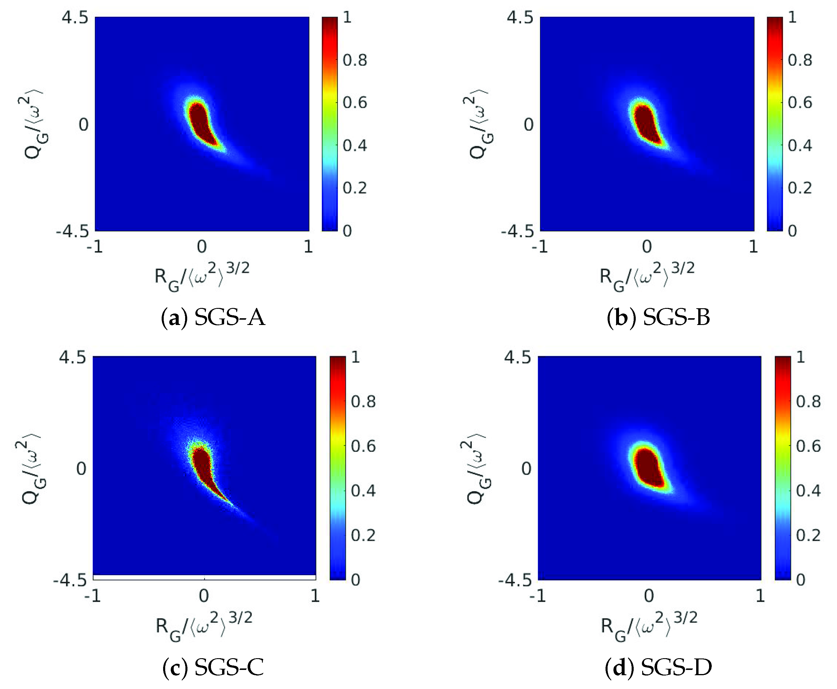
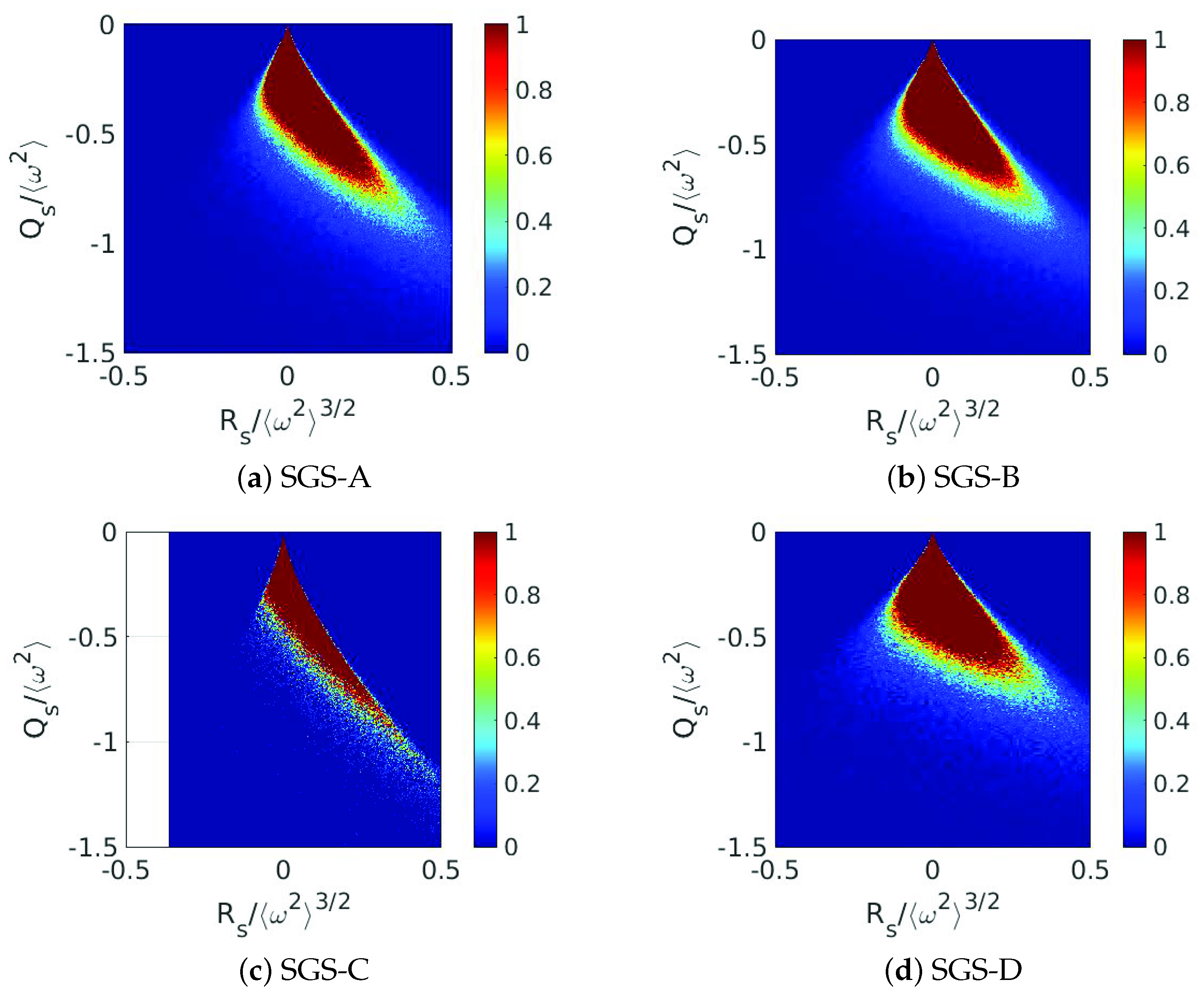
3.4.1. Dynamics of Filtered Velocity Gradients

The ( R G , Q G ) diagram in Figure 4a indicates that a fluid region with Q G > 0 consists of isolated whirled eddies intermittently dispersed with coherent activity of high vorticity. These eddies are stretched (compressed) if R G < 0 ( R G > 0 ) [45]. The Kelvin–Helmholtz theorem implies that the vorticity ω ( t ) of a vortex tube of length L ( t ) increases as it stretches; i.e., conservation of circulation is equivalent to, i.e., ω ( t ) / ω ( 0 ) = L ( t ) / L ( 0 ) . Figure 4b displays approximately 20 % positive deviation of Q G colored with R G where the turbulence field has been obtained by LES at a resolution of 256 3 grid points and Reynolds number R e = 3.14 × 10 6 . It indicates that large-magnitude vorticity mostly occurs in tubes ( R G < 0 ), which are intermittently dispersed with coherent regions of high vorticity ( ω ( t ) = 4 Q G + 2 Tr S 2 ). Vortex tubes are surrounded by high strain rate (in empty region Q G < 0 ). It is well known that vortex tubes appear like ‘spaghetti on a plate’—details of which are not resolved in LES because the number of grid points 256 3 considered in the simulation is relatively small with respect to R e = 3.14 × 10 6 .
The velocity gradient tensor illuminates the local topology of the flow resolved at the length scale Δ les . The equation of the velocity gradient tensor is derived by taking the gradient of Equation (2),
D G i j D t = G i k G k j 1 3 G m n G n m δ i j 2 P ¯ x i x j 1 3 2 P ¯ δ i j + ν 2 G i j x j x j 2 τ i j x j x j
where we have assumed that 2 P ¯ = 2 Q G . Terms on the right-hand side of Equation (12), except the two within the first pair of round brackets, represent the interaction with the velocity gradients of other surrounding fluid particles. The most important feature of the dynamics of the velocity gradient tensor is given by
D D t 1 2 G i j G i j = 1 4 ω i S i j ω j S i j S j k S k i .
Clearly, the local rate of production of the velocity gradient depends on the alignment between the vorticity and the eigenvector of strain rate tensor, ω i S i j ω j = ω 2 λ i ( e i · e ω ) 2 . Here, e i and e ω are strain rate eigenvectors and vorticity unit vectors, respectively. Based on Betchov’s relations [29], the average amount of strain self-amplification is three times the vortex stretching; i.e., ( 3 / 4 ) ω i S i j ω j = S i j S j k S k i . Hence
D D t G i j G i j = 2 ω i S i j ω j .
Thus, Equation (12) indicates that the energy cascade is governed by vortex stretching, which also depends on strain self-amplification (see also [15]).

3.4.2. Statistics

A compact and relatively convenient way to analyze the influence of the filtered velocity gradient tensor is the following five-dimensional dynamical systems of the invariants [2,14,32]:
d Q G d t = 3 R G d R G d t = 2 3 ( Q G ) 2 d Q S d t = 2 R S R G d R S d t = 2 3 Q G Q S + 1 4 V 2 d V 2 d t = 16 3 ( R S R G ) Q G .
Here, Q S = ( 1 / 2 ) S i j S i j , R S = ( 1 / 3 ) S i j S j k S k i , and the magnitude of the vortex stretching vector is V = | S ω | . It can also be seen that the first two of the system of equations are decoupled from the remaining three equations. Clearly, Q G increases if R G < 0 , and vice versa. Notably, it is a high-dimensional dynamical system, e.g., with 5 × 256 3 degrees of freedom if 256 3 cells are considered in the computation.
The histograms of R G and Q G are shown in Figure 5 and Figure 6. In studying the statistical theory, the kurtosis of a probability distribution usually measures the level of intermittency of an event. Distributions with large kurtosis exhibit tail data exceeding the tails of the normal distribution. For each of the four subgrid models tested, the histograms are distributed with high values of kurtosis. Observed kurtosis factors of R G and Q G are larger than 3, which implies a non-Gaussian leptokurtic distribution regardless of the choice of the subgrid model. Each model indicates the existence of extreme events making the bulk of the data in a skinny vertical range. From the histograms of R G , the relatively large kurtosis ( 56 –60) implies that the energy flux in two of the models, i.e., SGS-A and SGS-B, is relatively more intermittent and governed by vortex stretching. On the other hand, the histograms of R G form the other two models, i.e., SGS-C and SGS-D, indicate a relatively Gaussian, yet leptokurtic, distribution of the energy flux.
The overall flow topology and the resulting statistics manifested in Figure 5 and Figure 6 imply that there exist predominant spotty regions. Such local regions are characterized by strong vortices, as well as large amplitude fluctuations of the total strain. The non-Gaussian behavior with relatively large kurtosis depicted in Figure 5b,c implies that turbulent flows predicted with SGS-A and SGS-B are relatively more spotty compared to SGS-C and SGS-D. In other words, a high probability of large velocity derivatives—associated with the local mechanism of predominant vortex stretching—dies out through the globally averaged dynamics considered in SGS-C and SGS-D.

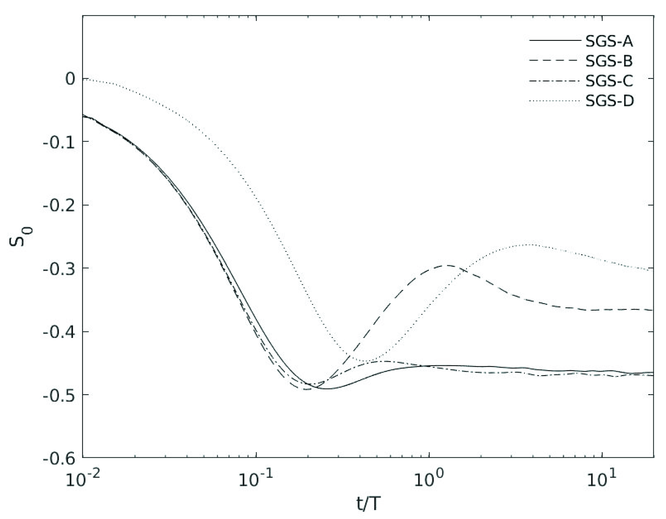
3.4.3. Energy Flux, Vortex Stretching, and Strain Skewness

In Figure 7, the joint PDF of R G and Q G shows that the bulk of the instantaneous velocity field is primarily in two quadrants: R G < 0 , Q G > 0 and R G > 0 , Q G < 0 . In the literature, the ( R G , Q G ) map was thoroughly scrutinized by many researchers suggesting that there is a sharp division between the vortex dominated region Q G > 3 ( R G ) 2 / 4 3 and strain-dominated region Q G < 3 ( R G ) 2 / 4 3 .
The ( R G , Q G ) map in Figure 7 shows a strong negative correlation, i.e., Q G R G < 0 . The ( R G , Q G ) map also provides some quantitative measure of the energy flux from large to small scales, Equation (7), i.e., Π = c k Δ 2 [ R G + ( 1 / 3 ) ω i ω j S i j ] and Π = c k Δ 2 ω i ω j S i j . The ( R G , Q G ) map among four subgrid models supports a good correlation between the energy cascade and vortex stretching, and that the two most common topological states of the flow are vortex stretching ω i ω j S i j > 0 and unstable sheet λ 1 λ 2 λ 3 < 0 [32,34]. It is worth mentioning that histograms of R G and Q G provide quantitative information regarding the vortex stretching mechanism, whereas the ( R G , Q G ) map provides the predominant role of vortex tubes and sheets.
In Figure 8, the ( R S , Q S ) invariant map compares the contribution of subgrid-scale stresses to the energy cascade. The invariant, Q S = ( 1 / 4 ) ε / ν , represents the viscous dissipation ε [32]. Large eddies with a negative values of Q S contribute to dissipation. The invariant R S is a special form of the invariant R G relative to the strain-dominated region Q G < 3 ( R G ) 2 / 4 3 of the ( R G , Q G ) map. For an incompressible flow, the eigenvalues of strain tensor S satisfy λ 1 λ 2 λ 3 and λ 1 + λ 2 + λ 3 = 0 . Thus, we can write R S = λ 1 λ 2 λ 3 . Similar to Equation (12), we have the following evolution equation
D D t 1 2 S i j S i j = S i j S j k S k i 1 4 ω i ω j S i j S i j 2 P x i x j + ν S i j 2 S i j .
The ( R S , Q S ) invariant map in Figure 8 along with Equation (14) provides a quantitative measure of how the rate of change of Q S = ( 1 / 2 ) S i j S i j depends on R S = ( 1 / 3 ) S i j S j k S k i , as well as on the rate of enstrophy production by vortex stretching, ω i ω j S i j . The main message from Equation (14) and Figure 8 is that positive values of R S or λ 1 λ 2 λ 3 < 0 correspond to production of S i j S i j by the strain self-amplification process. Thus, R S > 0 also implies that sheet-like structures are associated with viscous dissipation with λ 1 , λ 2 > 0 , and λ 3 < 0 . On the other hand, destruction of S i j S i j may correspond only marginally to tube-like structures due to λ 1 > 0 and λ 2 , λ 3 < 0 [15].
In accordance with [48] and other investigations, strain itself is induced by vorticity because there is no other way of production of enstrophy other than straining of weak vorticity. This mechanism is called self-amplification of velocity gradient tensor. In order to link this mechanism to the energy cascade, we focus on the statistics of the rate of vortex stretching
ω = ω i ω j S i j | ω |
and the second invariant of the rotation-rate tensor Q R . The statistics of these quantities appear directly in the vorticity equation
D 1 2 | ω | 2 D t = ω i ω j S i j + ν ω i 2 ω i .
Figure 9 shows some common features of the self-amplification of velocity derivatives. More specifically, the joint PDFs of the rate of vortex stretching ω with Q R show that the highest values of the enstrophy are associated with positive but low values of ω . High rates of vortex stretching and compression correlate with low values of enstrophy. The tilt towards positive values of ω implies that vortex tubes are being more stretched than compressed. Additionally, most of the volume in the fluid is occupied by relatively ‘weak’ vorticity, whereas strong vortices filling only a small fraction of the space. This feature is the most important ingredient for turbulence modeling, which is also depicted in Figure 5b,c.

4. Conclusions and Future Direction

In this article, we have analyzed the effects of four eddy-viscosity models on the statistical properties of energy transfer between resolved and subgrid scales in homogeneous isotropic turbulence. We have considered the classical approach, where dynamic variation of the energy flux is retrieved from the magnitude of strain rates. We have compared the statistical quantities from the classical method with that in which the energy flux is retrieved from the vortex stretching mechanism. Our mathematical and statistical analyses show that vortex stretching is the main mechanism driving the local energy cascade in isotropic turbulence. Local growth of both the strain and the rotation rates is directly influenced by the stretching of vorticity. The strain field is self-amplified if an isolated region of locally rotating fluid is stretched. Such a self-amplification of the strain contributes directly to the growth of absolute strain instead of enstrophy. Our numerical results imply that together vortex stretching rate and the effects of vortex stretching to an imbalance between strain and rotation rates govern the local rate of energy cascade.
Over the past half a century, the performance of subgrid models in LES has been thoroughly scrutinized by considering the contribution of strain self-amplification into the energy-flux. It has been 25 years since Meneveau [16] introduced primary statistical characteristics of subgrid models, which are often considered either in the formulation or the evaluation of subgrid models. This article compares statistics of the velocity gradient tensor in isotropic turbulence, which were computed using four subgrid models. We show that the statistics predicted by the Lagrangian dynamic model (SGS-D), where the model constant is dynamically calculated, are similar to the statistics predicted with the TKE-based dynamic model (SGS-C) in which fixed values of the model constants are assigned. We propose forming a subgrid-scale model of the energy flux, which is based on the vortex stretching mechanism. We have observed that the Kurtosis of the third invariant of the velocity gradient tensor is about three times as large if the subgrid model directly (e.g., SGS-A) or dynamically (e.g., SGS-B) captures the vortex stretching mechanism.
Two-point statistics, such as velocity increments and structure functions, are widely used in the study of turbulent flows [2,4]. In the present study, the filtered velocity gradients encompass the information contained in two-point statistics. The analysis of two-point statistics via velocity gradients suggests that vortex stretching rate correlates with the energy dissipation rate, particularly in the present investigation.
In future work, we are interested in considering the effects of different filtering strategies while vortex stretching is employed to retrieve the statistical properties of the energy flux in wall-bounded and thermally driven anisotropic turbulence. It may be interesting to investigate the wavelet-based filtering approach (e.g., our previous work [49]) with the vortex stretching approach presented in this article. A fully developed atmospheric boundary layer over an array of utility-scale wind turbine would help to assess efficiency of the subgrid model while considering an appropriate wall-modeling technique. This work is currently underway.

Author Contributions

Conceptualization and methodology, J.M.A. and A.M.V.; software, J.M.A.; validation, M.K.H.; writing—original draft preparation, M.K.H.; writing—review and editing, J.M.A. All authors have read and agreed to the published version of the manuscript.

Funding

This research was funded by NSERC discovery grant awarded to A.M.V. and The APC was funded by MUN.

Institutional Review Board Statement

Not applicable.

Informed Consent Statement

Not applicable.

Data Availability Statement

The data that support the findings of this study are generated by solving Navier-Stokes equations.

Acknowledgments

M.K.H. acknowledges financial support from the school of Graduate Studies, Memorial University, Canada. J.A. acknowledges the resource allocation grant from Compute Canada. A.M.V. acknowledges financial support from Natural Science and Research Council (NSERC) of Canada in form of a discovery grant.

Conflicts of Interest

The authors declare no conflict of interest.

Abbreviations

The following abbreviations are used in this manuscript:
CFDComputational Fluid Dynamics
LESLarge Eddy Simulation

References

  1. Bradshaw, P. Understanding and prediction of turbulent flow—1996. Int. J. Heat Fluid Flow 1997, 18, 45–54. [Google Scholar] [CrossRef]
  2. Davidson, P.A. Turbulence: An Introduction for Scientists and Engineers; Oxford University Press: Oxford, UK, 2004. [Google Scholar]
  3. Moser, R.D.; Haering, S.W.; Yalla, G.R. Statistical Properties of Subgrid-Scale Turbulence Models. Annu. Rev. Fluid Mech. 2021, 53, 255–286. [Google Scholar] [CrossRef]
  4. Pope, S.B. Turbulent flows; Cambridge University Press: Cambridge, UK, 2001. [Google Scholar]
  5. Meneveau, C.; Lund, T.S.; Cabot, W.H. A Lagrangian dynamic subgrid-scale model of turbulence. J. Fluid Mech. 1996, 319, 353–385. [Google Scholar] [CrossRef] [Green Version]
  6. Smagorinsky, J. General circulation experiments with the primitive equations: I. The basic experiment. Mon. Weather Rev. 1963, 91, 99–164. [Google Scholar] [CrossRef]
  7. Bazilevs, Y.; Michler, C.; Calo, V.; Hughes, T. Weak Dirichlet boundary conditions for wall-bounded turbulent flows. Comput. Methods Appl. Mech. Eng. 2007, 196, 4853–4862. [Google Scholar] [CrossRef]
  8. Golshan, R.; Tejada-Martínez, A.E.; Juha, M.; Bazilevs, Y. Large-eddy simulation with near-wall modeling using weakly enforced no-slip boundary conditions. Comput. Fluids 2015, 118, 172–181. [Google Scholar] [CrossRef] [Green Version]
  9. Piomelli, U.; Balaras, E. Wall-Layer Models For Large-Eddy Simulations. Annu. Rev. Fluid Mech. 2002, 34, 349–374. [Google Scholar] [CrossRef] [Green Version]
  10. Chung, D.; Pullin, D.I. Large-eddy simulation and wall modelling of turbulent channel flow. J. Fluid Mech. 2009, 631, 281–309. [Google Scholar] [CrossRef] [Green Version]
  11. Bose, S.T.; Park, G.I. Wall-Modeled Large-Eddy Simulation for Complex Turbulent Flows. Annu. Rev. Fluid Mech. 2018, 50, 535–561. [Google Scholar] [CrossRef]
  12. Eyink, G.L. Multi-scale gradient expansion of the turbulent stress tensor. J. Fluid Mech. 2006, 549, 159–190. [Google Scholar] [CrossRef] [Green Version]
  13. Tsinober, A. An Informal Introduction to Turbulence; Springer: Berlin/Heidelberg, Germany, 2001; Volume 63. [Google Scholar]
  14. Sagaut, P.; Cambon, C. Homogeneous Turbulence Dynamics; Cambridge University Press: Cambridge UK, 2018. [Google Scholar]
  15. Carbone, M.; Bragg, A.D. Is vortex stretching the main cause of the turbulent energy cascade? J. Fluid Mech. 2020, 883. [Google Scholar] [CrossRef] [Green Version]
  16. Meneveau, C. Statistics of turbulence subgrid-scale stresses: Necessary conditions and experimental tests. Phys. Fluids 1994, 6, 815–833. [Google Scholar] [CrossRef]
  17. Farge, M.; Schneider, K. Coherent Vortex Simulation (CVS), A Semi-Deterministic Turbulence Model Using Wavelets. Flow Turbul. Combust. 2001, 66, 393–426. [Google Scholar] [CrossRef]
  18. Doan, N.A.K.; Swaminathan, N.; Davidson, P.A.; Tanahashi, M. Scale locality of the energy cascade using real space quantities. Phys. Rev. Fluids 2018, 3, 084601. [Google Scholar] [CrossRef] [Green Version]
  19. Bhuiyan, M.A.S.; Alam, J.M. Scale-adaptive turbulence modeling for LES over complex terrain. Eng. Comput. 2020. [Google Scholar] [CrossRef]
  20. Alam, J.M.; Fitzpatrick, L.P. Large eddy simulation of flow through a periodic array of urban-like obstacles using a canopy stress method. Comput. Fluids 2018, 171, 65–78. [Google Scholar] [CrossRef]
  21. Alam, J.M.; Afanassiev, A.; Singh, J. Characterizing Impacts of Atmospheric Turbulence on Wind Farms Through Large Eddy Simulation (LES). In Ocean Renewable Energy, Proceedings of the International Conference on Offshore Mechanics and Arctic Engineering, Glasgow, Scotland, UK, 9–14 June 2019; American Society of Mechanical Engineers: New York, NY, USA, 2019; Volume 10. [Google Scholar]
  22. Borue, V.; Orszag, S.A. Local energy flux and subgrid-scale statistics in three-dimensional turbulence. J. Fluid Mech. 1998, 366, 1–31. [Google Scholar] [CrossRef]
  23. Taylor, G.I. The transport of vorticity and heat through fluids in turbulent motion. Proc. R. Soc. London. Ser. Contain. Pap. Math. Phys. Character 1932, 135, 685–702. [Google Scholar]
  24. Taylor, G.I. Production and dissipation of vorticity in a turbulent fluid. Proc. R. Soc. London. Ser. Math. Phys. Sci. 1938, 164, 15–23. [Google Scholar]
  25. Onsager, L. Statistical hydrodynamics. Il Nuovo C. (1943–1954). 1949, Volume 6, pp. 279–287. Available online: http://fig.if.usp.br/~marchett/fluidos/statistical-hydrodynamics_onsager.pdf (accessed on 28 November 2021).
  26. Bernard, P.S.; Thangam, S.; Speziale, C.G. The Role of Vortex Stretching in Turbulence Modeling. In Instability, Transition, and Turbulence; Springer: Berlin/Heidelberg, Germany, 1992; pp. 563–574. [Google Scholar]
  27. Kundu, P.K.; Cohen, I.M.; Dowling, D. Fluid Mechanics, 6th ed.; Academic Press: London, UK, 2016. [Google Scholar]
  28. Tennekes, H.; Lumley, J.L. A First Course in Turbulence; MIT Press: Cambridge, MA, USA, 2018. [Google Scholar]
  29. Betchov, R. An inequality concerning the production of vorticity in isotropic turbulence. J. Fluid Mech. 1956, 1, 497–504. [Google Scholar] [CrossRef]
  30. Shetty, D.A.; Frankel, S.H. Assessment of stretched vortex subgrid-scale models for LES of incompressible inhomogeneous turbulent flow. Int. J. Numer. Methods Fluids 2013, 73, 152–171. [Google Scholar] [CrossRef] [Green Version]
  31. Nicoud, F.; Ducros, F. Subgrid-scale stress modelling based on the square of the velocity gradient tensor. Flow Turbul. Combust. 1999, 62, 183–200. [Google Scholar] [CrossRef]
  32. Trias, F.; Folch, D.; Gorobets, A.; Oliva, A. Building proper invariants for eddy-viscosity subgrid-scale models. Phys. Fluids 2015, 27, 065103. [Google Scholar] [CrossRef] [Green Version]
  33. Martın, J.; Ooi, A.; Chong, M.S.; Soria, J. Dynamics of the velocity gradient tensor invariants in isotropic turbulence. Phys. Fluids 1998, 10, 2336–2346. [Google Scholar] [CrossRef]
  34. da Silva, C.B.; Pereira, J.C. Invariants of the velocity-gradient, rate-of-strain, and rate-of-rotation tensors across the turbulent/nonturbulent interface in jets. Phys. Fluids 2008, 20, 055101. [Google Scholar] [CrossRef] [Green Version]
  35. Lund, T.S.; Novikov, E. Parameterization of subgrid-scale stress by the velocity gradient tensor. Annu. Res. Briefs 1992, 1992, 27–43. [Google Scholar]
  36. Germano, M.; Piomelli, U.; Moin, P.; Cabot, W.H. A dynamic subgrid-scale eddy viscosity model. Phys. Fluids Fluid Dyn. 1991, 3, 1760–1765. [Google Scholar] [CrossRef] [Green Version]
  37. McMillan, O.J.; Ferziger, J.H. Direct Testing of Subgrid-Scale Models. AIAA J. 1979, 17, 1340–1346. [Google Scholar] [CrossRef] [Green Version]
  38. Deardorff, J.W. A numerical study of three-dimensional turbulent channel flow at large Reynolds numbers. J. Fluid Mech 1970, 41, 453–480. [Google Scholar] [CrossRef]
  39. Deardorff, J.W. The Use of Subgrid Transport Equations in a Three-Dimensional Model of Atmospheric Turbulence. J. Fluids Eng. 1973, 95, 429–438. [Google Scholar] [CrossRef]
  40. Deardorff, J.W. Stratocumulus-capped mixed layers derived from a three-dimensional model. Bound.-Layer Meteorol. 1980, 18, 495–527. [Google Scholar] [CrossRef]
  41. Stoll, R.; Gibbs, J.A.; Salesky, S.T.; Anderson, W.; Calaf, M. Large-Eddy Simulation of the Atmospheric Boundary Layer. Bound.-Layer Meteorol. 2020, 177, 541–581. [Google Scholar] [CrossRef]
  42. Yoshizawa, A. Statistical theory for compressible turbulent shear flows, with the application to subgrid modeling. Phys. Fluids 1986, 29, 2152–2164. [Google Scholar] [CrossRef]
  43. Bardina, J.; Ferziger, J.; Reynolds, W. Improved subgrid-scale models for large-eddy simulation. In Proceedings of the 13th Fluid and Plasma Dynamics Conference, Snowmass, CO, USA, 14–16 July 1980. [Google Scholar]
  44. Comte-Bellot, G.; Corrsin, S. Simple Eulerian time correlation of full-and narrow-band velocity signals in grid-generated, isotropic turbulence. J. Fluid Mech. 1971, 48, 273–337. [Google Scholar] [CrossRef]
  45. Dallas, V.; Alexakis, A. Structures and dynamics of small scales in decaying magnetohydrodynamic turbulence. Phys. Fluids 2013, 25, 105106. [Google Scholar] [CrossRef] [Green Version]
  46. Liu, S.; Meneveau, C.; Katz, J. On the properties of similarity subgrid-scale models as deduced from measurements in a turbulent jet. J. Fluid Mech. 1994, 275, 83–119. [Google Scholar] [CrossRef]
  47. Kolmogorov, A.N. A refinement of previous hypotheses concerning the local structure of turbulence in a viscous incompressible fluid at high Reynolds number. J. Fluid Mech. 1962, 13, 82–85. [Google Scholar] [CrossRef] [Green Version]
  48. Jiménez, J.; Wray, A.A.; Saffman, P.G.; Rogallo, R.S. The structure of intense vorticity in isotropic turbulence. J. Fluid Mech. 1993, 255, 65–90. [Google Scholar] [CrossRef] [Green Version]
  49. Alam, J.; Islam, M.R. A multiscale eddy simulation methodology for the atmospheric Ekman boundary layer. Geophys. Astrophys. Fluid Dyn. 2015, 109, 1–20. [Google Scholar] [CrossRef]
Figure 1. A comparison of the time history of the velocity gradient skewness S 0 among four subgrid models.
Aerospace 08 00375 g001
Figure 2. Comparisons of the second moment of the velocity field among 4 subgrid models. (a) E ( t ) / E ( 0 ) and t 10 / 7 . (b) k sgs and t 10 / 7 . (c) E ( k ) at t / T = 3 and k 5 / 3 .
Aerospace 08 00375 g002aAerospace 08 00375 g002b
Figure 3. A plot of the time series of the rate of change of the resolved energy, d E / d t (block …), the energy flux τ i j S i j (black ), the viscous dissipation rate ϵ (red ), and the mean enstrophy ω 2 (black ——).
Aerospace 08 00375 g003
Figure 4. (a) A schematic illustration of the invariant map ( R G , Q G ) , which illustrates that the vorticity dominates over the rate of strain in the region D > 0 for D ( 27 / 4 ) ( R G ) 2 + ( Q G ) 3 [34]. (b) Isosurface plot of 20 % positive deviation of Q G , which is colored by R G for a turbulent flow simulated on 256 3 grid points using the vortex stretching-based model SGS-A, Equation (9).
Aerospace 08 00375 g004
Figure 5. (a) A schematic illustration of mesokurtic (Kurtosis = 3), leptokurtic (kurtosis > 3) and platykurtic (kurtosis < 3) distribution. (be) A comparison of the probability density function of R G – the third invariant of the velocity gradient tensor G – among the subgrid models SGS-A (b), SGS-B (c), SGS-C (d), and SGS-D (e) (see Table 1).
Aerospace 08 00375 g005
Figure 6. A comparison of the probability density function of Q G , the second invariant of the velocity gradient tensor G with respect to subgrid models SGS-A (a), SGS-B (b), SGS-C (c), and SGS-D (d) (see Table 1).
Aerospace 08 00375 g006
Figure 7. A comparison of the joint probability density function of two invariants Q G and R G of the velocity gradient tensor G with respect to subgrid models SGS-A (a), SGS-B (b), SGS-C (c), and SGS-D (d) (see Table 1).
Aerospace 08 00375 g007
Figure 8. A comparison of the joint probability density function of two invariants R S and Q S of the strain rate tensor S with respect to subgrid models SGS-A (a), SGS-B (b), SGS-C (c), and SGS-D (d).
Aerospace 08 00375 g008
Figure 9. The joint probability density of second invariants ω and Q ω (i.e., Q R ) of two tensors S and R , respectively, where the results are compared among 4 subgrid models: SGS-A (a), SGS-B (b), SGS-C (c), and SGS-D (d).
Aerospace 08 00375 g009
Table 1. A comparison for the values of λ , η , R e λ , and ϵ predicted from the LES data corresponding to 4 subgrid models at a resolution of 128 3 cells.
ModelRemark λ η R e λ ϵ
SGS-ANicoud and Ducros [31]0.11055.9719 × 10 4 88370.0629
SGS-BYoshizawa [42]0.07965.0677 × 10 4 63650.1231
SGS-CDeardorff [39]0.10685.8718 × 10 4 85460.0673
SGS-DMeneveau et al. [5]0.08805.3308 × 10 4 70430.0991
Publisher’s Note: MDPI stays neutral with regard to jurisdictional claims in published maps and institutional affiliations.

