Movement Characteristics of a Dual-Spin Guided Projectile Subjected to a Lateral Impulse

Abstract

In this paper, a new dual-spin guided projectile that is equipped with ten lateral impulse jets is proposed for trajectory correction. To guide the overall design of the projectile and the control system, a linear motion model of the projectile that was subjected to a lateral impulse was obtained based on a full nonlinear seven-degree-of-freedom (7-DOF) dynamic model. The trajectory correction process of a lateral impulse was divided into two stages. To explain the principle of lateral impulse trajectory correction, the analytical solutions of the linear model of these two stages were obtained. Analytical and numerical solutions were compared to verify the accuracy of the linear model. It is concluded that the analytical and numerical solutions are in good agreement.

1. Introduction

Over the past several decades, due to the extreme acceleration loads at launch and the high spin rate during the entire trajectory, minimizing the terminal miss distance and collateral damage of spin-stabilized projectiles has been a great challenge. Fortunately, with the advance of low cost, small, rugged, microelectronic mechanical systems, a significant reduction in the dispersion for direct fire projectiles that are equipped with a relatively inexpensive flight control system is possible. For spin-stabilized projectiles, however, the extremely high spin rate causes other technical problems [1]. Firstly, due to the high spin rate it is hard to measure the attitude angles of spin-stabilized projectiles. Secondly, the control mechanism that is used for spin-stabilized projectiles should have high power and bandwidth. Finally, the flight dynamics of spin-stabilized projectiles are relatively complex.

A classical strategy to overcome the aforementioned problems is the dual-spin projectile with four fixed canards that are mounted on the fuse. This dual-spin projectile (also called a Precision Guidance Kit (PGK)) is composed of the forward part with a low spin rate to reduce the canard actuator power and bandwidth, as well as the aft part with a high spin rate to maintain the stability of the entire projectile. Many dual-spin projectile studies have been published such as the linear theory [2,3,4], aerodynamic characteristics [5,6,7], flight mechanics [8,9,10,11,12], and the control method [13,14,15]. Nevertheless, the introduction of control surfaces complicates the dynamics of the projectile. Consequently, this brings new challenges and increases the cost of the overall projectile design.

Compared to the control surface, the impulse jet that delivers a large, short-duration impulse to the body represents a simpler and less costly control mechanism. Impulse jets have been applied to modify the trajectory of spacecrafts [16,17] and subsequently they have been applied to rockets [18,19,20,21,22] and missiles [23,24,25]. These objects are all low-speed and are low-spin rate fin-stabilized projectiles whose movement characteristics are relatively simple. For spin-stabilized projectiles, the action time of the impulse jets is not short enough and the action force is not strong enough. Therefore, impulse jets are seldom used as a control mechanism for spin-stabilized projectiles.

In this paper, a new dual-spin projectile with impulse jets is proposed to correct the trajectory of the conventional spin-stabilized projectile. The new projectile consists of two parts that are connected by a bearing. A new rigid body seven-degree-of-freedom (7-DOF) model including nonlinear aerodynamic forces and moments is explained in Section 2. The exact numerical solution of this model can be obtained by the fourth-order Runge–Kutta method for the initial conditions. However, when compared to a numerical solution, an analytical solution can demonstrate the effect of the physical and aerodynamic parameters on dynamics [26]. Therefore, analytical solutions can help to understand the movement characteristics of the projectile more completely and to design the control system more easily.

Based on the rigid body 6-DOF motion differential equations, the linear angular motion equation was established for spin-stabilized projectiles in the complex plane in [26,27]. The analytical solution was also obtained. This analytical theory was extended to include the effect of a lateral impulse for a fin-stabilized projectile in [18]. The action of a lateral impulse was modeled as a generalized lateral translation and angular disturbances which were incorporated into the linear angular motion equation directly. In [20], the action of a lateral impulse was regarded as the initial conditions of the linear angular motion equation. In addition, the ignition process of an impulse jet was simplified by neglecting the aerodynamic forces and moments. The form of the linear angular motion equation was not changed in [18,20] because the research objects were both 6-DOF. For a dual-spin projectile, however, the linear angular motion equation needs to be deduced again. To keep the nonlinearity of the equation as much as possible, the impulse force and moment are modeled into the 7-DOF motion differential equations. Thus, the linear angular motion equation can predict the whole movement characteristics of a 7-DOF projectile subjected a lateral impulse.

The paper is organized as follows: A 7-DOF nonlinear dynamic model, including nonlinear aerodynamic forces and moments, is explained in detail in Section 2. The linear angular motion equations that are based on the model that is established in Section 2 are derived in Section 3. Analytical solutions of the dual-spin projectile motion equations that are subjected to a lateral impulse are obtained in Section 4. Lastly, the simulation results on a 155 mm dual-spin projectile are presented in Section 5 to verify the accuracy of the theoretical derivation that is provided in Section 3 and Section 4.

2. Nonlinear Dynamics Model

The projectile dynamic model and the methodology that are used for the forces and moments on the projectile are described in this section.

2.1. Concept Design and Reference Frames

The high spin rate of spin-stabilized projectiles brings great challenges to attitude measurement and trajectory control. Inspired by PGK, a dual-spin structure was adopted. The measurement and control components were arranged on a de-spin body (aft body), while the projectile body (forward body) was characterized by a high spin rate to maintain the stability of the entire projectile. Since the impulse jets were mounted behind the center of mass of spin-stabilized projectiles, the boattail of a projectile was transformed into a guided boattail connected to the projectile body avia a bearing. To reduce the spin rate of a guided boattail, six inclined fins were mounted on it. All electronic devices and control mechanisms were located inside the guide boattail. The overall structure of the dual-spin projectile is shown in Figure 1.

After the projectile was launched, the spin rate of the guided boattail quickly decreased due to the six inclined fins. An onboard Global Positioning System (GPS) measured the position and velocity information of the projectile. Based on this information, the projectile’s computer predicts the projectile’s impact point. When deviation between the predicted impact point and the ideal impact point satisfies certain conditions, the projectile computer gives an ignition order to the appropriate impulse jet to correct the trajectory of the projectile.

The aforementioned structure was relatively simple and easy to implement; only the boattail of a projectile needed to be redesigned. This means that the modification of the aerodynamic characteristics of the projectile was minor and some of the original aerodynamic parameters of the projectile can still be employed. On the other hand, due to the relative simplicity of the control mechanism, only the GPS and a three-axis geomagnetic sensor were used for navigation. To maximize the correction ability of the projectile and achieve precision guidance, the movement characteristics of the projectile that was subjected to a lateral impulse under different conditions have to be investigated in detail.

Two reference frames are introduced below to describe the projectile movement. One is the ground reference frame $O_{\mathrm{N}}{x}_{\mathrm{N}}{y}_{\mathrm{N}}{z}_{\mathrm{N}}$ (Figure 2a), and the other one is the no-roll reference frame $Oxyz$ which is fixed to the projectile (Figure 2b). The origin ($O_{\mathrm{N}}$) of the ground reference frame was located at the launch point. $O_{\mathrm{N}}{x}_{\mathrm{N}}$ is the axis launch direction in the horizontal plane, and the $O_{\mathrm{N}}{y}_{\mathrm{N}}$ axis is oriented in the upright direction. The $O_{\mathrm{N}}{z}_{\mathrm{N}}$ axis can be determined by the right-hand rule. The origin $O$ of the no-roll reference frame is the center of the projectile mass. The $Ox$ axis aligns with the projectile axis and points to the nose, thus defining a positive direction. The $Oy$ axis is perpendicular to the $Ox$ axis in the horizontal plane. Like the $O_{\mathrm{N}}{z}_{\mathrm{N}}$ axis, the $Oz$ axis can be determined by the right-hand rule. The reference frames are shown in Figure 2.

Linear $(u,v,w)$ and angular $(p_{\mathrm{f}},p_{\mathrm{a}},q,r)$ velocities are the system dynamic states which are described in the no-roll reference frame. The linear $(x_{\mathrm{e}},y_{\mathrm{e}},z_{\mathrm{e}})$ and angular $({\varphi }_{\mathrm{f}},{\varphi }_{\mathrm{a}},\theta ,\psi )$ positions are the system kinematic states which are described in the ground reference frame [15]. The relationship between the total velocity and the projectile axis is described by the angle of attack (AOA) $\alpha$ and the angle of sideslip (AOS) $\beta$. The relationships between them can be expressed as:

$$\{\begin{array}{l}\left|V\right|=\sqrt{u^2+v^2+w^2},\alpha =\arctan \left(\frac{w}{u}\right)\\ \beta =\arcsin \left(-\frac{v}{V}\right)=\arctan \left(\frac{-v}{\sqrt{u^2+w^2}}\right)\end{array}$$

(1)

2.2. Nonlinear Dynamics Model

The 7-DOF nonlinear model for the dual-spin projectiles that were employed in this paper was established in [2]. According to the introduction of the reference frames in Section 2.1, the kinematic equations of the projectile can be expressed as:

$$\left[\begin{array}{c}{\dot{x}}_{\mathrm{e}}\\ {\dot{y}}_{\mathrm{e}}\\ {\dot{z}}_{\mathrm{e}}\end{array}\right]=\left[\begin{array}{ccc}\cos \theta \cos \psi & -\sin \psi & \sin \theta \cos \psi \\ \sin \theta & 0& -\cos \theta \\ \cos \theta \sin \psi & \cos \psi & \sin \theta \sin \psi \end{array}\right]\left[\begin{array}{c}u\\ v\\ w\end{array}\right]$$

(2)

$$\left[\begin{array}{c}{\dot{\varphi }}_{\mathrm{f}}\\ {\dot{\varphi }}_{\mathrm{a}}\\ \dot{\theta }\\ \dot{\psi }\end{array}\right]=\left[\begin{array}{cccc}1& 0& 0& \tan \theta \\ 0& 1& 0& \tan \theta \\ 0& 0& 1& 0\\ 0& 0& 0& 1/\cos \theta \end{array}\right]\left[\begin{array}{c}{p}_{\mathrm{f}}\\ p_{\mathrm{a}}\\ q\\ r\end{array}\right]$$

(3)

The dynamic equations of the projectile can be expressed as:

$$\left[\begin{array}{c}\dot{u}\\ \dot{v}\\ \dot{w}\end{array}\right]=\frac{1}{m}\left[\begin{array}{c}{F}_{\mathrm{x}}\\ F_{\mathrm{y}}\\ F_{\mathrm{z}}\end{array}\right]+\left[\begin{array}{c}rv-qw\\ -rw\tan \theta -ru\\ qu+rv\tan \theta \end{array}\right]$$

(4)

$$\left[\begin{array}{c}{\dot{p}}_{\mathrm{f}}\\ {\dot{p}}_{\mathrm{a}}\\ \dot{q}\\ \dot{r}\end{array}\right]=I^{-1}\left(\left[\begin{array}{c}{M}_{\mathrm{xf}}\\ M_{\mathrm{xa}}\\ M_{\mathrm{y}}\\ M_{\mathrm{z}}\end{array}\right]-\left[\begin{array}{cccc}0& 0& -r& q\\ 0& 0& -r& q\\ r& r& 0& r\tan \theta \\ -q& -q& -r\tan \theta & 0\end{array}\right]I\left[\begin{array}{c}{p}_{\mathrm{f}}\\ p_{\mathrm{a}}\\ q\\ r\end{array}\right]\right)$$

(5)

where $F_{\mathrm{x}}$, $F_{\mathrm{y}}$, and $F_{\mathrm{z}}$ are the projections of the external force of the projectile on $Ox$, $Oy$, and $Oz$ axes, respectively. $M_{\mathrm{xf}}$ ($M_{\mathrm{xa}}$), $M_{\mathrm{y}}$, and $M_{\mathrm{z}}$ are the projections of the external moment of the projectile on $Ox$, $Oy$, and $Oz$ axes, respectively. The symbol $m$ represents the mass of the projectile. Matrix ${\rm I}$ is the inertia matrix of the projectile relative to the $Oxyz$ reference frame. The matrix can be specifically expressed as:

$$I=\left[\begin{array}{cccc}{I}_{\mathrm{xf}}& 0& 0& 0\\ 0& I_{\mathrm{xa}}& 0& 0\\ 0& 0& I_{\mathrm{y}}& 0\\ 0& 0& 0& I_{\mathrm{z}}\end{array}\right]$$

(6)

where $I_{\mathrm{xf}}$ and $I_{\mathrm{xa}}$ are the main axes of inertia of the projectile body and the boattail relative to the $Ox$ axis. $I_{\mathrm{y}}$ and $I_{\mathrm{z}}$ are the main axes of inertia of the entire projectile relative to the $Oy$, and $Oz$ axes, respectively.

2.3. Forces and Moments

2.3.1. Forces

The force that is acting on the projectile in Equation (4) is comprised of the aerodynamic force, the weight force, and the impulse force $F_{\mathrm{i}}$. A combination of the force in the no-roll reference frame can be expressed as:

$$F=\frac{1}{2}\rho V^{2}S\left(C_{\mathrm{D}}\left[\begin{array}{c}-\cos \beta \cos \alpha \\ -\sin \beta \\ -\cos \beta \sin \alpha \end{array}\right]+C_{\mathrm{L}}\left[\begin{array}{c}{\sin }^2\beta +{\cos }^2\beta {\sin }^2\alpha \\ -\cos \beta \sin \beta \cos \alpha \\ -{\cos }^2\beta \sin \alpha \cos \alpha \end{array}\right]\right)+mg\left[\begin{array}{c}-\sin \theta \\ 0\\ \cos \theta \end{array}\right]+F_{\mathrm{i}}$$

(7)

where $\rho$ is the air density, $S$ is the reference area, $C_{\mathrm{D}}$ is the drag force coefficient, $C_{\mathrm{L}}$ is the lift force coefficient, and $g$ is the gravitational acceleration.

2.3.2. Moments

The moment that is acting on the projectile body and the boattail is described in Equation (5) and is comprised of the aerodynamic moment, the friction moment $M_{\mathrm{s}}$ of the bearing, and the impulse control moment $M_{\mathrm{i}}$. A combination of the moment in the no-roll reference frame can be expressed as:

$$M=\frac{1}{2}\rho VSL\left[\begin{array}{c}-VD{C}_{\mathrm{SDf}}{p}_{\mathrm{f}}\\ -VD{C}_{\mathrm{SDa}}{p}_{\mathrm{a}}+V{C}_{\mathrm{S}}\epsilon \\ V{C}_{\mathrm{P}}\cos \beta \sin \alpha -D{C}_{\mathrm{M}}\sin \beta -D{C}_{\mathrm{PD}}q\\ -V{C}_{\mathrm{P}}\sin \beta -D{C}_{\mathrm{M}}\cos \beta \sin \alpha -D{C}_{\mathrm{PD}}r\end{array}\right]+M_{\mathrm{s}}+M_{\mathrm{i}}$$

(8)

where $L$ is the reference length, $D$ is the projectile diameter, $\epsilon$ is the oblique angle of incline fins, $C_{\mathrm{SDf}}$ and $C_{\mathrm{SDa}}$ are the spin damping moment coefficients of the forward and aft body, respectively, $C_{\mathrm{S}}$ is the spin moment coefficient of incline fins, $C_{\mathrm{P}}$ is the pitching moment coefficient, $C_{\mathrm{M}}$ is the Magnus moment coefficient, and $C_{\mathrm{PD}}$ is the pitching damping moment coefficient.

2.3.3. Forces and Moments of Impulse Jets

The force that is due to the impulse jet in the no-roll reference frame can be expressed as:

$$F_{\mathrm{i}}=\left[\begin{array}{c}0\\ F_{\mathrm{p}}\cos (\gamma +{\varphi }_{\mathrm{a}})\\ F_{\mathrm{p}}\sin (\gamma +{\varphi }_{\mathrm{a}})\end{array}\right]$$

(9)

where $\gamma$ is the fixing angle of the impulse jet.

The moment that is due to the impulse jet in the no-roll reference frame can be expressed as:

$$M_{\mathrm{i}}=\left[\begin{array}{c}0\\ 0\\ F_{\mathrm{p}}r\sin \left(\gamma +{\varphi }_{\mathrm{a}}\right)\\ -F_{\mathrm{p}}r\cos \left(\gamma +{\varphi }_{\mathrm{a}}\right)\end{array}\right]$$

(10)

where $r$ is the distance from the impulse jet nozzle to the center of projectile mass.

2.3.4. Friction Moment of Bearing

The friction moments of the bearing to the projectile body and the boattail are equal in value but are opposite in direction [15]. The friction moment in the no-roll reference frame can be expressed as:

$$M_{\mathrm{s}}=\frac{1}{2}\rho V^{2}SD\left[\begin{array}{c}{C}_{\mathrm{A}}\mathrm{sgn}\left(p_{\mathrm{a}}-p_{\mathrm{f}}\right)\left(K_{\mathrm{S}}+K_{\mathrm{V}}\left|p_{\mathrm{a}}-p_{\mathrm{f}}\right|\right)\\ -C_{\mathrm{A}}\mathrm{sgn}\left(p_{\mathrm{a}}-p_{\mathrm{f}}\right)\left(K_{\mathrm{S}}+K_{\mathrm{V}}\left|p_{\mathrm{a}}-p_{\mathrm{f}}\right|\right)\\ 0\\ 0\end{array}\right]$$

(11)

where $C_{\mathrm{A}}$ is the axial force coefficient, and $K_{\mathrm{S}}$ and $K_{\mathrm{V}}$ are the static and viscous friction coefficients of bearings, respectively.

3. Linearized Angular Motion Model

The dynamic equations of the projectile that were established in Section 2 are highly nonlinear. Numerical solutions can be obtained by the fourth-order Runge–Kutta for given initial conditions. However, analytical solutions that show the explicit relationships between all parameters cannot easily be obtained. Without analytical solutions, the dynamic characteristics of dual-spin projectiles cannot be adequately comprehended. In this section, linear equations of the angular motion and the velocity direction of the projectile were derived from the nonlinear motion equations that were based on certain assumptions. Moreover, the solutions to these linear equations were also obtained. Analytical solutions of linear equations can accurately and intuitively explain the projectile motion, especially for the movement characteristics that are subjected to a lateral impulse.

3.1. Assumptions for Linearization

• The projectile is mass balanced, such that the centers of gravity of both the projectile body and the boattail lie on the rotational axis of symmetry and $I_{\mathrm{y}}=I_{\mathrm{z}}$;
• The spin rates of the projectile body and the boattail are constant during the ignition;
• The change of projectile mass characteristics that are caused by the impulse jet ignition is ignored;
• The aerodynamic angles of attack are small so that $\alpha \approx w/V$, $\beta \approx -v/V$;
• The quantities $V$ and $u$ are large compared to $q$, $r$, $v$, and $w$, such that products of the small quantities and their derivatives are negligible;
• The projectile is aerodynamically symmetrical;
• The thrust force of the impulse jet is constant and there is no ignition delay.

3.2. Projectile Motion Parameters Described in the Complex Field

Any point $O_{\mathrm{c}}$ along the direction of the velocity vector of the projectile is first chosen. Then, a complex plane that is perpendicular to the velocity vector passing through the point $O_{\mathrm{c}}$ is created. The intersection of the $Ox$ axis and the complex plane is defined as the point $B$. Vector $O_{\mathrm{c}}B$ represents the total AOA in the complex plane (see Figure 3a). In the same way, the intersection of the changing velocity vector and the complex plane is defined as the point $E$. Vector $O_{\mathrm{c}}E$ represents the velocity deflection angle in the complex plane (see Figure 3b). When the total AOA of the projectile changes, the trajectory of the point $B$ in the complex plane reflects this change. Analogously, the trajectory of the point $E$ in the complex plane can reflect the change in the velocity direction.

The total AOA $\Delta$ and the velocity deflection angle $\Psi$ are relatively small in magnitude. As such, they can be expressed as:

$$\{\begin{array}{l}\Delta =\frac{1}{V}\left(w+\mathrm{i}v\right)\approx \alpha -\mathrm{i}\beta \\ \Psi ={\psi }_{\mathrm{a}}+\mathrm{i}{\psi }_{\mathrm{d}}\end{array}$$

(12)

These two quantities can be expressed in polar coordinates as:

$$\{\begin{array}{l}\Delta =\left|\Delta \right|{\mathrm{e}}^{\mathrm{i}\varphi }\\ \Psi =\left|\Psi \right|{\mathrm{e}}^{\mathrm{i}\phi }\end{array}$$

(13)

3.3. Derivation of the Linear Angular Motion Equation

The parameter $\dot{x}$ indicates the derivative of the example variable $x$ with respect to time, while $x^{\prime }$ stands for the derivative of the variable $x$ with respect to ballistic arc length. The relationship between the aforementioned parameters is given as:

$$\dot{x}=\frac{\mathrm{d}x}{\mathrm{d}t}=\frac{\mathrm{d}x}{\mathrm{d}s}\cdot \frac{\mathrm{d}s}{\mathrm{d}t}=x^{\prime }\cdot V$$

(14)

where $t$ is time and $s$ is the ballistic arc length.

By employing the method that is described in Equation (14), the independent variable $t$ is replaced with $s$ in the second and third lines of Equation (4). Then, these values are divided by $V^2$. The parameters $rw\tan \theta$ and $rv\tan \theta$ are negligible relative to $ru$ and $qu$. Therefore, these two equations can be written as:

$$\{\begin{array}{l}\frac{1}{V}{v}^{\prime }=\frac{F_{\mathrm{y}}}{m{V}^2}-\frac{ru}{V^2}\\ \frac{1}{V}{w}^{\prime }=\frac{F_{\mathrm{z}}}{m{V}^2}+\frac{qu}{V^2}\end{array}$$

(15)

The first line in Equation (15) is multiplied by a negative imaginary unit and added to the second line. Thus, the following expression is obtained:

$$\frac{1}{V}\left(w^{\prime }-\mathrm{i}{v}^{\prime }\right)=\frac{1}{m{V}^2}\left(F_{\mathrm{z}}-\mathrm{i}{F}_{\mathrm{y}}\right)+\frac{u}{V}\left(\frac{q}{V}+\mathrm{i}\frac{r}{V}\right)$$

(16)

The first line in Equation (12) is differentiated with respect to the arc length:

$$\frac{\mathrm{d}\Delta }{\mathrm{d}s}=-\frac{1}{V^2}\left(w-\mathrm{i}v\right)\frac{\mathrm{d}V}{\mathrm{d}s}+\frac{1}{V}\left(w^{\prime }-\mathrm{i}{v}^{\prime }\right)$$

(17)

Equations (16) and (17) are combined to obtain:

$$\frac{\mathrm{d}\Delta }{\mathrm{d}s}=-\frac{\Delta }{V}\frac{\mathrm{d}V}{\mathrm{d}s}+\frac{1}{m{V}^2}\left(F_{\mathrm{z}}-\mathrm{i}{F}_{\mathrm{y}}\right)+\frac{u}{V}\left(\frac{q}{V}+\mathrm{i}\frac{r}{V}\right)$$

(18)

Under the assumption that $u/V\approx 1$ and by defining $\frac{1}{V}\left(r-\mathrm{i}q\right)=\Phi$, Equation (18) can be rewritten as:

$${\Delta }^{\prime }+\frac{V^{\prime }}{V}\Delta -\mathrm{i}\Phi =\frac{1}{m{V}^2}\left(F_{\mathrm{z}}-\mathrm{i}{F}_{\mathrm{y}}\right)$$

(19)

By employing Equation (14), the independent variable $t$ is replaced with $s$ in the third and fourth lines of Equation (5) and divided by $V^2$. The parameters $r^2\tan \theta$ and $rq\tan \theta$ are negligible relative to $pr$ and $pq$. Hence, these two equations can be expressed as:

$$\{\begin{array}{l}\frac{1}{V}{q}^{\prime }=\frac{M_{\mathrm{y}}}{V^2{I}_{\mathrm{y}}}-\frac{I_{\mathrm{xf}}{p}_{\mathrm{f}}+I_{\mathrm{xa}}{p}_{\mathrm{a}}}{V{I}_{\mathrm{y}}}\frac{r}{V}\\ \frac{1}{V}{r}^{\prime }=\frac{M_{\mathrm{z}}}{V^2{I}_{\mathrm{z}}}+\frac{p_{\mathrm{f}}{I}_{\mathrm{xf}}+I_{\mathrm{xa}}{p}_{\mathrm{a}}}{V{I}_{\mathrm{z}}}\frac{q}{V}\end{array}$$

(20)

The first line in Equation (20) is multiplied by a negative imaginary unit and added to the second line:

$$\frac{1}{V}\left(r^{\prime }-\mathrm{i}{q}^{\prime }\right)=\frac{1}{V^2{I}_{\mathrm{y}}}\left(M_{\mathrm{z}}-\mathrm{i}{M}_{\mathrm{y}}\right)+\frac{I_{\mathrm{xf}}{p}_{\mathrm{f}}+I_{\mathrm{xa}}{p}_{\mathrm{a}}}{V{I}_{\mathrm{z}}}\left(\frac{q}{V}+\mathrm{i}\frac{r}{V}\right)$$

(21)

The parameter $\Phi$ is differentiated with respect to the arc length:

$${\Phi }^{\prime }=-\frac{V^{\prime }}{V^2}\left(r-\mathrm{i}q\right)+\frac{\left(r^{\prime }-\mathrm{i}{q}^{\prime }\right)}{V}$$

(22)

By substituting Equation (22) into Equation (21), and defining $P$ as $P=\frac{I_{\mathrm{xf}}{p}_{\mathrm{f}}+I_{\mathrm{xa}}{p}_{\mathrm{a}}}{V{I}_{\mathrm{z}}}$, the following expression is obtained:

$${\Phi }^{\prime }=-\frac{V^{\prime }}{V}\Phi +\frac{1}{V^2{I}_{\mathrm{y}}}\left(M_{\mathrm{z}}-\mathrm{i}{M}_{\mathrm{y}}\right)+\mathrm{i}P\Phi$$

(23)

Then, Equation (19) can be rewritten as:

$$\mathrm{i}\Phi ={\Delta }^{\prime }+\frac{V^{\prime }}{V}\Delta -\frac{1}{m{V}^2}\left(F_{\mathrm{z}}-\mathrm{i}{F}_{\mathrm{y}}\right)$$

(24)

Equation (19) can be differentiated with respect to the arc length:

$${\Delta }^{″}+\frac{V^{\prime }}{V}{\Delta }^{\prime }+\left(\frac{V^{″}}{V}-\frac{{V^{\prime }}^2}{V^2}\right)\Delta -\mathrm{i}{\Phi }^{\prime }=\frac{1}{m{V}^2}\left({F^{\prime }}_{\mathrm{z}}-\mathrm{i}{F^{\prime }}_{\mathrm{y}}\right)-\frac{2V^{\prime }}{m{V}^3}\left(F_{\mathrm{z}}-\mathrm{i}{F}_{\mathrm{y}}\right)$$

(25)

Equations (23) and (24) are substituted into Equation (25), while higher-order terms are assumed as negligible:

$${\Delta }^{″}+\left(\frac{2V^{\prime }}{V}-\mathrm{i}P\right){\Delta }^{\prime }+\left(\frac{V^{″}}{V}-\mathrm{i}P\frac{V^{\prime }}{V}\right)\Delta =\frac{{F^{\prime }}_{\mathrm{z}}-\mathrm{i}{F^{\prime }}_{\mathrm{y}}}{m{V}^2}-\mathrm{i}\frac{P\left(F_{\mathrm{z}}-\mathrm{i}{F}_{\mathrm{y}}\right)}{m{V}^2}+\frac{\mathrm{i}\left(M_{\mathrm{z}}-\mathrm{i}{M}_{\mathrm{y}}\right)}{V^2{I}_{\mathrm{y}}}$$

(26)

According to Equations (7) and (8), some aerodynamic forces and moments can be rewritten in the complex form:

$$\{\begin{array}{l}{F}_{\mathrm{z}}-\mathrm{i}{F}_{\mathrm{y}}=-m{k}_{\mathrm{d}}{V}^2\Delta -m{k}_{\mathrm{l}}{V}^2\Delta +mg\cos \theta -\mathrm{i}{F}_{\mathrm{p}}{\mathrm{e}}^{\mathrm{i}\left({\varphi }_{\mathrm{a}}+\gamma \right)}\\ M_{\mathrm{z}}-\mathrm{i}{M}_{\mathrm{y}}=-I_{\mathrm{y}}{k}_{\mathrm{p}}{V}^2\left(\mathrm{i}\Delta \right)-I_{\mathrm{y}}{k}_{\mathrm{pd}}{V}^2\Phi -I_{\mathrm{y}}{k}_{\mathrm{m}}V\Delta -F_{\mathrm{p}}r{\mathrm{e}}^{\mathrm{i}\left({\varphi }_{\mathrm{a}}+\gamma \right)}\end{array}$$

(27)

where

$$\{\begin{array}{l}{k}_{\mathrm{d}}=\frac{\rho S}{2m}{C}_{\mathrm{D}},k_{\mathrm{l}}=\frac{\rho S}{2m}{C}_{\mathrm{L}}\\ k_{\mathrm{p}}=\frac{\rho SL}{2I_{\mathrm{y}}}{C}_{\mathrm{P}},k_{\mathrm{pd}}=\frac{\rho SLD}{2I_{\mathrm{y}}}{C}_{\mathrm{PD}},k_{\mathrm{m}}=\frac{\rho SLD}{2I_{\mathrm{y}}}{C}_{\mathrm{M}}\end{array}$$

(28)

In the direction along the velocity vector, drag force and gravity are dominant components. Hence:

$$\dot{V}=-k_x{V}^2-g\sin \theta$$

(29)

According to Equation (14), Equation (19) can be rewritten as:

$$\frac{V^{\prime }}{V}=-k_x-\frac{g\sin \theta }{V^2}$$

(30)

Equations (27)–(30) are substituted into Equation (26) to obtain:

$${\Delta }^{″}+\left(H-\mathrm{i}P\right){\Delta }^{\prime }-\left(M+\mathrm{i}PT\right)\Delta =\tilde{G}+\tilde{I}$$

(31)

where

$$\{\begin{array}{l}H=k_{\mathrm{pd}}+k_{\mathrm{l}}-k_{\mathrm{d}}-2\frac{g\sin \theta }{V^2},M=k_{\mathrm{p}}\\ T=k_{\mathrm{l}}-k_{\mathrm{m}}\frac{p_{\mathrm{f}}}{VP},\tilde{G}=-\frac{\ddot{\theta }}{V^2}-\left(k_{\mathrm{pd}}-\mathrm{i}P\right)\frac{\dot{\theta }}{V}\\ K_{\mathrm{I}}=\left[\frac{mr}{A}-\left(k_{\mathrm{pd}}-\mathrm{i}P\right)-\mathrm{i}\frac{p_{\mathrm{a}}}{v}\right]\frac{F_{\mathrm{p}}}{m{v}^2}{\mathrm{e}}^{\mathrm{i}\left({\varphi }_{\mathrm{a}0}+\gamma \right)}\\ \tilde{I}=K_{\mathrm{I}}{\mathrm{e}}^{\mathrm{i}{p}_{\mathrm{a}}s/V}\end{array}$$

(32)

where ${\varphi }_{\mathrm{a}0}$ is the rolling angle of the boattail at the start of the ignition.

In Equation (31), $\tilde{G}$ stands for the gravity action in a complex number field, while $\tilde{I}$ stands for the impulse action.

3.4. Analysis Solutions of the Linear Angular Motion Equation

Equation (31) is a second-order non-homogeneous linear differential equation. Its general solution consists of two parts; one part is a special solution of the non-homogeneous linear equation itself and the other part is the general solution of the homogeneous linear equation corresponding to the equation. The general solution of Equation (31) can be expressed as:

$$\Delta =K_{\mathrm{F}0}{\mathrm{e}}^{{\lambda }_{\mathrm{F}}s+\mathrm{i}\left({\omega }_{\mathrm{F}}s+{\varphi }_{\mathrm{F}0}\right)}+K_{\mathrm{S}0}{\mathrm{e}}^{{\lambda }_{\mathrm{S}}s+\mathrm{i}\left({\omega }_{\mathrm{S}}s+{\varphi }_{\mathrm{S}0}\right)}+{\Delta }^{*}$$

(33)

The first two terms of Equation (33) represent the general solutions of the homogeneous linear equation corresponding to Equation (31), while the third term is a special solution. According to Equation (33), the general solution of the homogeneous linear equation corresponding to Equation (31) is the superposition of two circular motions (respectively defined as fast circular motion and slow circular motion). Parameters $K_{\mathrm{F}0}$ and $K_{\mathrm{S}0}$ are the initial amplitudes of the fast and slow circular motions, ${\varphi }_{\mathrm{F}0}$, and ${\varphi }_{\mathrm{S}0}$ are the initial phase angles of fast and slow circular motions, ${\lambda }_{\mathrm{F}}$ and ${\lambda }_{\mathrm{S}}$ are the damping indices of fast and slow circular motions, and ${\omega }_{\mathrm{F}}$ and ${\omega }_{\mathrm{S}}$ are the angular frequencies of fast and slow circular motions, respectively. These values are defined in [26] as:

$${\omega }_{\mathrm{F}}=\frac{1}{2}\left(P+\sqrt{P^2-4M}\right)$$

(34)

$${\omega }_{\mathrm{S}}=\frac{1}{2}\left(P-\sqrt{P^2-4M}\right)$$

(35)

$${\lambda }_{\mathrm{F}}=-\frac{1}{2}\left(H-\frac{P\left(2T-H\right)}{\sqrt{P^2-4M}}\right)$$

(36)

$${\lambda }_{\mathrm{S}}=-\frac{1}{2}\left(H+\frac{P\left(2T-H\right)}{\sqrt{P^2-4M}}\right)$$

(37)

The angular movement of the projectile that is subjected to a lateral impulse can be divided into two stages. The first stage is the forced movement of the projectile that is subjected to a direct impulse force. The second stage is the free movement of the projectile immediately after the first stage under the action of the aerodynamic force and gravity. Analytical solutions of angular motion equations of these two stages are separately solved below.

4. Angular Motion of the Projectile Subjected to a Lateral Impulse

4.1. Angular Motion at the First Stage

Due to the superposition of the second-order non-homogeneous linear differential equations, the influence of gravity can be neglected when only the action of the impulse is studied. Hence, Equation (31) can be simplified as:

$${\Delta }^{″}+\left(H-\mathrm{i}P\right){\Delta }^{\prime }-\left(M+\mathrm{i}PT\right)\Delta =\tilde{I}=K_{\mathrm{I}}{\mathrm{e}}^{\mathrm{i}{p}_{\mathrm{a}}s/V}$$

(38)

Since the ignition time of the impulse jet is extremely short, the spin rate of the boattail can be assumed as constant during the ignition. In this situation, the right side of Equation (38) is an exponential forcing function. Therefore, the special solution is also an exponential function:

$${\Delta }^{*}=K_{\mathrm{I}0}{\mathrm{e}}^{\mathrm{i}\left({\omega }_{\mathrm{ax}}s+\gamma +{\varphi }_{\mathrm{a}0}\right)}=K_{\mathrm{I}}{\mathrm{e}}^{\mathrm{i}\left({\omega }_{\mathrm{ax}}s\right)}$$

(39)

where ${\omega }_{\mathrm{ax}}={{\varphi }^{\prime }}_{\mathrm{a}}=p_{\mathrm{a}}/V$.

By substituting Equation (39) into Equation (38), the following expression is obtained:

$$K_{\mathrm{I}}=\frac{I}{P{\omega }_{\mathrm{a}x}-{\omega }_{\mathrm{a}x}^2-M+\mathrm{i}\left({\omega }_{\mathrm{a}x}H-PT\right)}$$

(40)

An assumption is made that the projectile is flying steadily before the impulse jet is ignited. In other words, when $s=0$, $\Delta =0$ and ${\Delta }^{\prime }=0$. For these initial conditions, the following expression can be written:

$$\{\begin{array}{l}{K}_{\mathrm{F}}+K_{\mathrm{S}}+K_{\mathrm{I}}=0\\ K_{\mathrm{F}}\left({\lambda }_{\mathrm{F}}+\mathrm{i}{\omega }_{\mathrm{F}}\right)+K_{\mathrm{S}}\left({\lambda }_{\mathrm{S}}+\mathrm{i}{\omega }_{\mathrm{S}}\right)+\mathrm{i}{\omega }_{\mathrm{ax}}{K}_{\mathrm{I}}=0\end{array}$$

(41)

where:

$$\{\begin{array}{l}{K}_{\mathrm{F}}=K_{\mathrm{F}0}{\mathrm{e}}^{\mathrm{i}{\varphi }_{\mathrm{F}0}}\\ K_{\mathrm{S}}=K_{\mathrm{S}0}{\mathrm{e}}^{\mathrm{i}{\varphi }_{\mathrm{S}0}}\end{array}$$

(42)

Thus, the solution of Equation (41) is obtained as:

$$\{\begin{array}{l}{K}_{\mathrm{F}}=K_{\mathrm{I}}\frac{\left({\lambda }_{\mathrm{S}}+\mathrm{i}{\omega }_{\mathrm{S}}\right)-\mathrm{i}{\omega }_{\mathrm{a}x}}{\left({\lambda }_{\mathrm{F}}+\mathrm{i}{\omega }_{\mathrm{F}}\right)-\left({\lambda }_{\mathrm{S}}+\mathrm{i}{\omega }_{\mathrm{S}}\right)}\\ K_{\mathrm{S}}=-K_{\mathrm{I}}\frac{\left({\lambda }_{\mathrm{F}}+\mathrm{i}{\omega }_{\mathrm{F}}\right)-\mathrm{i}{\omega }_{\mathrm{a}x}}{\left({\lambda }_{\mathrm{F}}+\mathrm{i}{\omega }_{\mathrm{F}}\right)-\left({\lambda }_{\mathrm{S}}+\mathrm{i}{\omega }_{\mathrm{S}}\right)}\end{array}$$

(43)

At this point, the angular motion at the first stage can be obtained:

$$\Delta =K_{\mathrm{F}}{\mathrm{e}}^{{\lambda }_{\mathrm{F}}s+\mathrm{i}{\omega }_{\mathrm{F}}s}+K_{\mathrm{S}}{\mathrm{e}}^{{\lambda }_{\mathrm{S}}s+\mathrm{i}{\omega }_{\mathrm{S}}s}+K_{\mathrm{I}}{\mathrm{e}}^{\mathrm{i}{\omega }_{\mathrm{a}x}s}$$

(44)

Equation (44) is differentiated with respect to the arc length. Then, the angular velocity of the angle of attack is acquired:

$${\Delta }^{\prime }=K_{\mathrm{F}}\left({\lambda }_{\mathrm{F}}+\mathrm{i}{\omega }_{\mathrm{F}}\right){\mathrm{e}}^{{\lambda }_{\mathrm{F}}s+\mathrm{i}{\omega }_{\mathrm{F}}s}+K_{\mathrm{S}}\left({\lambda }_{\mathrm{S}}+\mathrm{i}{\omega }_{\mathrm{S}}\right){\mathrm{e}}^{{\lambda }_{\mathrm{S}}s+\mathrm{i}{\omega }_{\mathrm{S}}s}+\mathrm{i}{K}_{\mathrm{I}}{\omega }_{\mathrm{ax}}{\mathrm{e}}^{\mathrm{i}{\omega }_{\mathrm{ax}}s}$$

(45)

4.2. Angular Motion at the Second Stage

After the ignition is over, Equation (38) can be rewritten as:

$${\Delta }^{″}+\left(H-\mathrm{i}P\right){\Delta }^{\prime }-\left(M+\mathrm{i}PT\right)\Delta =0$$

(46)

Equation (46) is a homogeneous linear equation corresponding to Equation (31), and its general solution form is provided by Equation (33) as:

$$\Delta =K_{\mathrm{F}0}{\mathrm{e}}^{{\lambda }_{\mathrm{F}}s+\mathrm{i}\left({\omega }_{\mathrm{F}}s+{\varphi }_{\mathrm{F}0}\right)}+K_{\mathrm{S}0}{\mathrm{e}}^{{\lambda }_{\mathrm{S}}s+\mathrm{i}\left({\omega }_{\mathrm{S}}s+{\varphi }_{\mathrm{S}0}\right)}$$

(47)

Coefficients $K_{\mathrm{F}0}$ and $K_{\mathrm{S}0}$ in Equation (47) are determined based on the initial conditions. According to [26], the damping components in Equation (47) have a minor effect on the initial conditions. By deriving Equation (47) with respect to the arc length and assuming the negligible effect of the damping components in it, the following expression is obtained:

$${\Delta }^{\prime }=\left({\lambda }_{\mathrm{F}}+\mathrm{i}{\omega }_{\mathrm{F}}\right)K_{\mathrm{F}}{\mathrm{e}}^{\mathrm{i}{\omega }_{\mathrm{F}}s}+\left({\lambda }_{\mathrm{S}}+\mathrm{i}{\omega }_{\mathrm{S}}\right)K_{\mathrm{S}}{\mathrm{e}}^{\mathrm{i}{\omega }_{\mathrm{S}}s}$$

(48)

By combining Equations (47) and (48), the relationship between the initial angle of attack and the initial angular velocity of the angle of the attack, coefficients $K_{\mathrm{F}0}$, $K_{\mathrm{S}0}$ can be obtained:

$$\{\begin{array}{l}{K}_{\mathrm{F}}=\frac{{{\Delta }^{\prime }}_0-\left({\lambda }_{\mathrm{S}}+\mathrm{i}{\omega }_{\mathrm{S}}\right){\Delta }_0}{\left({\lambda }_{\mathrm{F}}-{\lambda }_{\mathrm{S}}\right)+\mathrm{i}\left({\omega }_{\mathrm{F}}-{\omega }_{\mathrm{S}}\right)}\\ K_{\mathrm{S}}=\frac{-{{\Delta }^{\prime }}_0+\left({\lambda }_{\mathrm{F}}+\mathrm{i}{\omega }_{\mathrm{F}}\right){\Delta }_0}{\left({\lambda }_{\mathrm{F}}-{\lambda }_{\mathrm{S}}\right)+\mathrm{i}\left({\omega }_{\mathrm{F}}-{\omega }_{\mathrm{S}}\right)}\end{array}$$

(49)

By substituting the initial conditions that are caused by the lateral impulse (see Equations (44) and (45)) into Equation (49), an analytical solution of the angular motion of the projectile at the second stage can be acquired:

$$\Delta =K_{\mathrm{F}}{e}^{{\lambda }_{\mathrm{F}}s+\mathrm{i}{\omega }_{\mathrm{F}}s}+K_{\mathrm{S}}{e}^{{\lambda }_{\mathrm{S}}s+\mathrm{i}{\omega }_{\mathrm{S}}s}$$

(50)

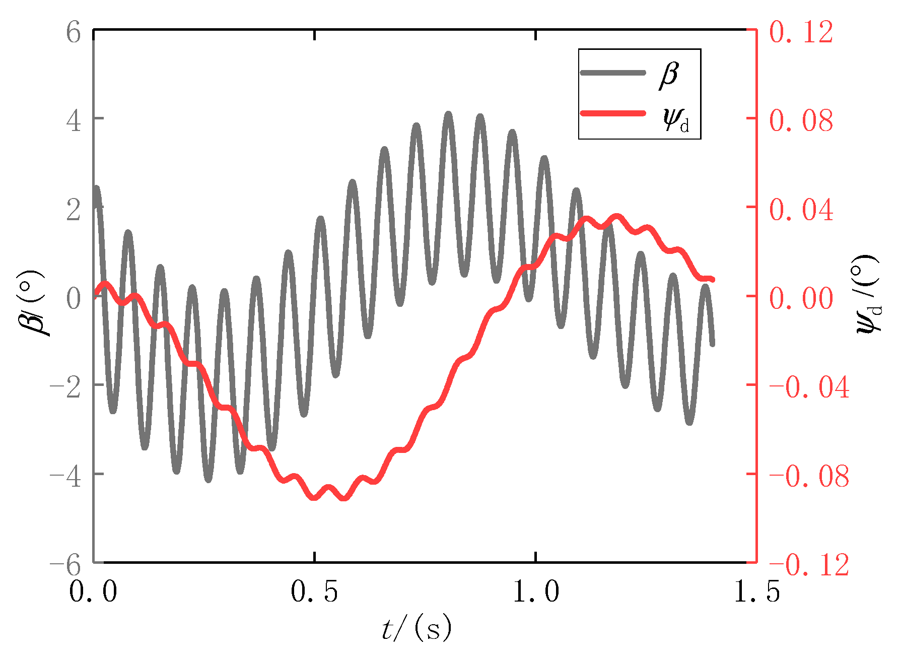
4.3. Deflection Angle of the Velocity at the First Stage

A complex deflection angle that is given in Section 3.2 is used for describing the deflection of the projectile velocity. The relationship between the complex deflection angle and the lift force is provided in [27]. The action of the lateral impulse should also be included. Thus, the following expression is obtained:

$$\dot{\Psi }=k_{\mathrm{l}}V\Delta +\frac{F_{\mathrm{p}}}{mV}{\mathrm{e}}^{\mathrm{i}\left({\omega }_{\mathrm{a}x}s+\gamma +{\varphi }_{\mathrm{a}0}\right)}$$

(51)

By substituting Equation (44) at the first stage into Equation (51), the following expression is acquired:

$$\dot{\Psi }=k_{\mathrm{l}}V\left(K_{\mathrm{F}}{\mathrm{e}}^{{\lambda }_{\mathrm{F}}s+\mathrm{i}{\omega }_{\mathrm{F}}s}+K_{\mathrm{S}}{\mathrm{e}}^{{\lambda }_{\mathrm{S}}s+\mathrm{i}{\omega }_{\mathrm{S}}s}+K_{\mathrm{I}}{\mathrm{e}}^{\mathrm{i}{\omega }_{\mathrm{ax}}s}\right)+\frac{F_{\mathrm{p}}}{mV}{\mathrm{e}}^{\mathrm{i}\left({\omega }_{\mathrm{a}x}s+\gamma +{\varphi }_{\mathrm{a}0}\right)}$$

(52)

A variable of integration in Equation (52) is replaced from the arc length to $Vt$ and the expression is integrated with time to obtain:

$$\Psi =\frac{k_{\mathrm{l}}{K}_{\mathrm{F}}\left(e^{{\lambda }_{\mathrm{F}}Vt+\mathrm{i}{\omega }_{\mathrm{F}}Vt}-1\right)}{{\lambda }_{\mathrm{F}}+\mathrm{i}{\omega }_{\mathrm{F}}}+\frac{k_{\mathrm{l}}{K}_{\mathrm{S}}\left({\mathrm{e}}^{{\lambda }_{\mathrm{S}}Vt+\mathrm{i}{\omega }_{\mathrm{S}}Vt}-1\right)}{{\lambda }_{\mathrm{S}}+\mathrm{i}{\omega }_{\mathrm{S}}}+\left[\frac{k_{\mathrm{l}}{K}_{\mathrm{I}}}{\mathrm{i}{\omega }_{\mathrm{ax}}}+\frac{F_{\mathrm{p}}{\mathrm{e}}^{\mathrm{i}\left(\gamma +{\varphi }_{\mathrm{a}0}\right)}}{\mathrm{i}m{\omega }_{\mathrm{ax}}{V}^2}\right]\left({\mathrm{e}}^{\mathrm{i}{\omega }_{\mathrm{ax}}Vt}-1\right)$$

(53)

4.4. Deflection Angle of the Velocity at the Second Stage

When the ignition of the impulse jet is over, Equation (51) can be rewritten as:

$$\dot{\Psi }=k_{\mathrm{l}}V\Delta$$

(54)

By substituting Equation (50) at the second stage into Equation (54), the following equation is obtained:

$$\dot{\Psi }=k_{\mathrm{l}}V\left(K_{\mathrm{F}}{e}^{{\lambda }_{\mathrm{F}}s+\mathrm{i}{\omega }_{\mathrm{F}}s}+K_{\mathrm{S}}{e}^{{\lambda }_{\mathrm{S}}s+\mathrm{i}{\omega }_{\mathrm{S}}s}\right)$$

(55)

Furthermore, a variable of integration is replaced from arc length to $vt$ and the expression is integrated with time to obtain:

$$\Psi =k_{\mathrm{l}}\left[\frac{K_{\mathrm{F}}\left(e^{{\lambda }_{\mathrm{F}}Vt+\mathrm{i}{\omega }_{\mathrm{F}}Vt}-1\right)}{{\lambda }_{\mathrm{F}}+\mathrm{i}{\omega }_{\mathrm{F}}}+\frac{K_{\mathrm{S}}\left(e^{{\lambda }_{\mathrm{S}}Vt+\mathrm{i}{\omega }_{\mathrm{S}}Vt}-1\right)}{{\lambda }_{\mathrm{S}}+\mathrm{i}{\omega }_{\mathrm{S}}}\right]$$

(56)

According to Equation (56), the complex deflection angle periodically swings with decreasing amplitude along the average deflection angle under the action of the damping terms. Finally, it stabilizes around the average deflection angle. By neglecting the periodic terms in Equation (56), the average deflection angle can be expressed as:

$$\overline{\Psi }=-k_{\mathrm{l}}\left(\frac{K_{\mathrm{F}}}{{\lambda }_{\mathrm{F}}+\mathrm{i}{\omega }_{\mathrm{F}}}+\frac{K_{\mathrm{S}}}{{\lambda }_{\mathrm{S}}+\mathrm{i}{\omega }_{\mathrm{S}}}\right)$$

(57)

5. Results and Discussion

Accurate numerical results of the trajectory with and without a lateral impulse can be obtained by numerically integrating the fully nonlinear equations. A comparison between these two situations was made on a 155-mm dual-spin projectile.

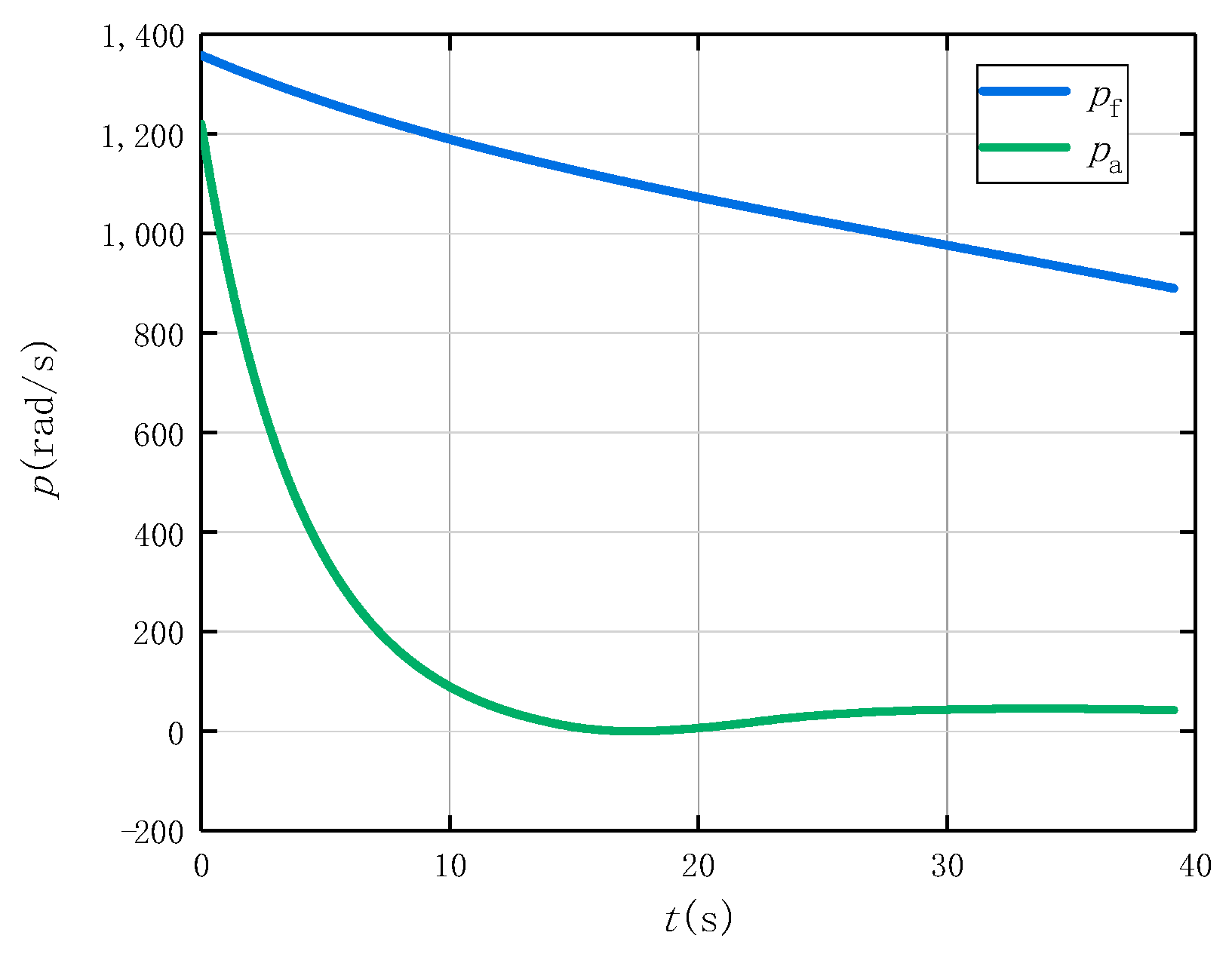
5.1. Numerical Simulation Results

The configuration of the projectile used for this investigation is shown in Figure 1, while the physical properties are summarized in

Table 1. Parameters of the dual-spin projectile (Mach 1.02).

Parameter	Value	Parameter	Value
Mass of projectile body	39.24 kg	$I_{\mathrm{y}}=I_{\mathrm{z}}$	1.61 kg·m2
Mass of boattail	7.80 kg	Drag force coefficient	0.3295
Diameter of projectile	0.155 m	Lift force coefficient	1.9589
Length of projectile body	0.790 m	Pitching moment coefficient	0.7752
Length of boattail	0.112 m	Magnus moment coefficient	−0.0491
$I_{\mathrm{xf}}$	0.14 kg·m2	Pitching damping moment coefficient	1.5251
$I_{\mathrm{xa}}$	0.02 kg·m2	Oblique angle of incline fins	−3 deg

. Parameters defining an impulse jet are listed in

Table 2. Parameters of the impulse jet.

Parameter	Value	Parameter	Value
$\gamma$	0 deg	${\varphi }_{\mathrm{a}0}$	0.3295
Thrust force	1400 N	Working time	20 ms
$r$	0.2065 m	$p_{\mathrm{a}}$	9.6851 rad/s

. For all cases, the numerical solutions were generated using a fixed step fourth-order Range–Kutta algorithm. The initial velocity of the projectile was 670 m/s, and the firing angle was 21 degrees. Two trajectories were obtained. One was a normal trajectory without any impulse jets being ignited, and the other one was a correcting trajectory with a single impulse jet being ignited. The average action angle of the ignited impulse jet was 90 degrees. Trajectories of the projectile are shown in Figure 4.

The difference of the impact points in the down-range was negligible, while the difference in the crossrange was 15 m.

The spin rate of forward and aft bodies is shown in Figure 5. The spin rate of the aft body decreased rapidly after firing and met the measurement and control requirements at approximately 10 s. Impulse action did not affect the spin rate. Thus, only a single case is shown in this figure.

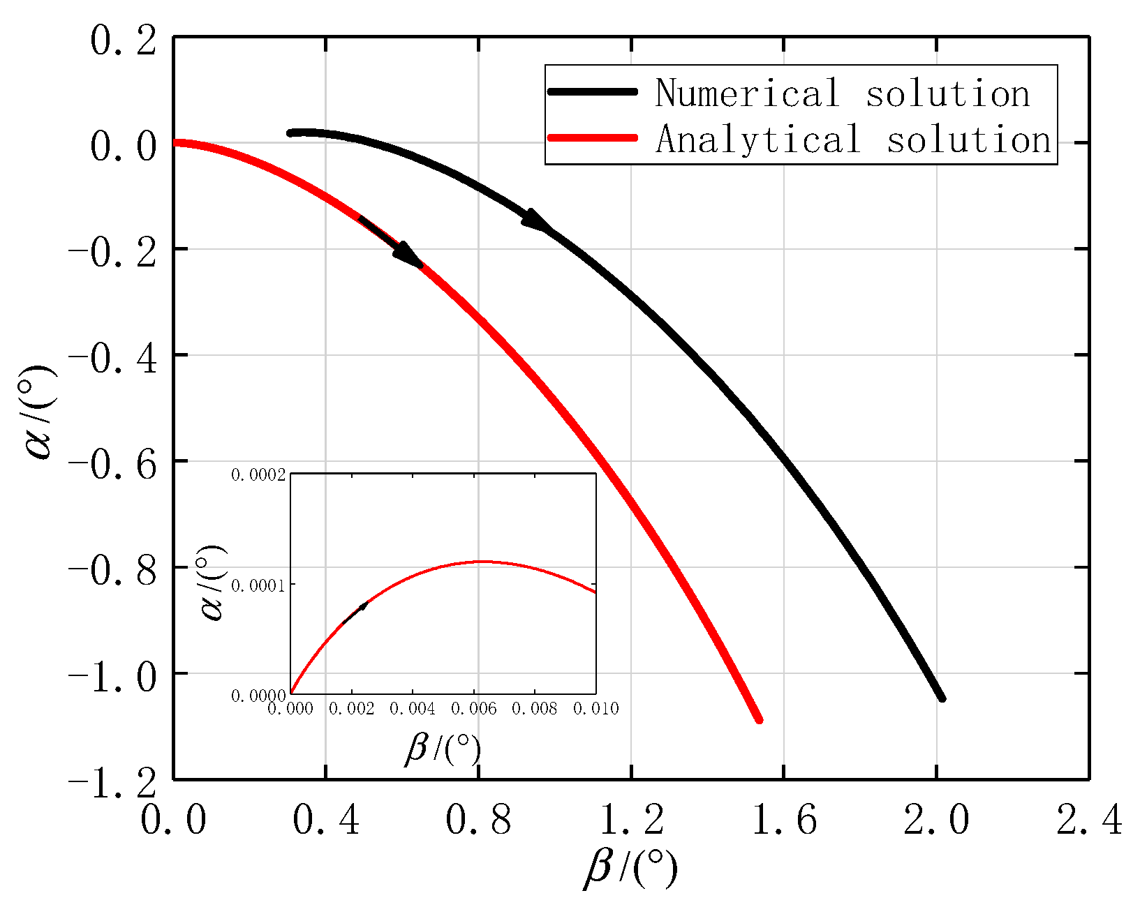
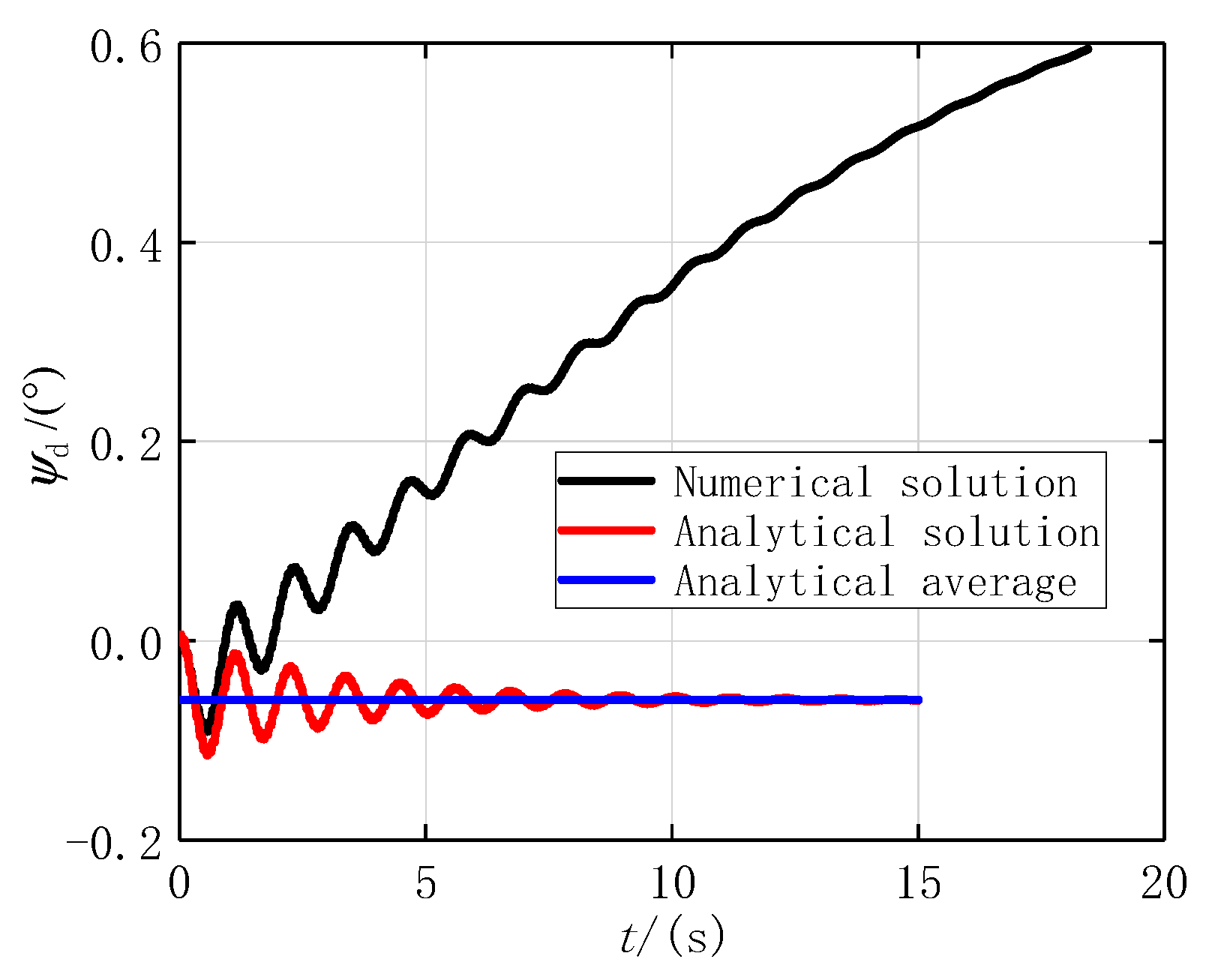
5.2. Numerical and Analytical Solutions at the First Stage

The angular motion of the projectile at the first stage is shown in Figure 6. The results obtained by the two methods are in good agreement. Since the actual initial total AOA of the projectile was not zero, a difference between the numerical and analytical solutions in angular motion was caused by the initial conditions. The difference increases with the increasing of the $\beta$ angle. That is because when the $\beta$ angle is large enough, the aerodynamic action works. The initial total AOA in the numerical solution was caused by gravity. This phenomenon is called dynamic equilibrium angle [27]. The black arrows on the curves indicate the angular motion direction. When the impulse jet was ignited at 84.4562 degrees, the projectile axis moved in the opposite direction of the impulse force from the origin, thus forming positive $\alpha$ and $\beta$ angles. According to Equation (44), the angular motion in the first stage should be a three circular motion. Moreover, the angular frequency of the fast circular motion was much higher than the frequency of other motions. Thus, the projectile axis moved in the direction where the value of $\alpha$ is negative and rapidly decreased.

The change in the velocity deflection angle at the first stage is shown in Figure 7. The two values of ${\psi }_{\mathrm{d}}$ that were obtained by the two methods were approximately equal to each other. A minor difference between them was caused by the gravity between the two values of ${\psi }_{\mathrm{a}}$. The value of ${\psi }_{\mathrm{a}}$ in the analytical solution became zero at the end of the first stage because the impulse action counteracted in this direction. The value of ${\psi }_{\mathrm{a}}$ in the numerical solution decreased at the whole first stage because of the gravity which was neglected in the analytical solution. Velocity deflection angle at this stage was formed by the combined action of impulse and aerodynamic forces. Since the total AOA was relatively small when coupled with a small aerodynamic lift force, the impulse force was dominant at this stage.

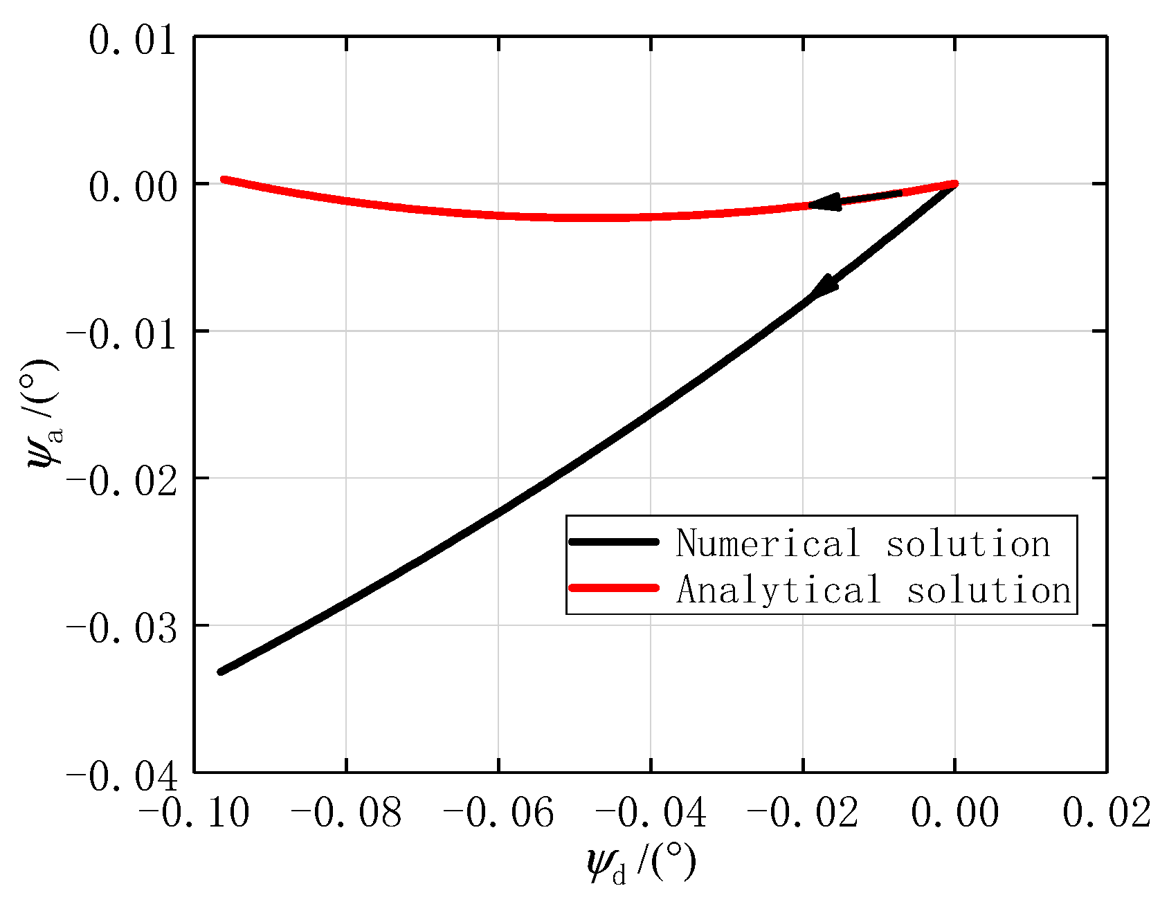
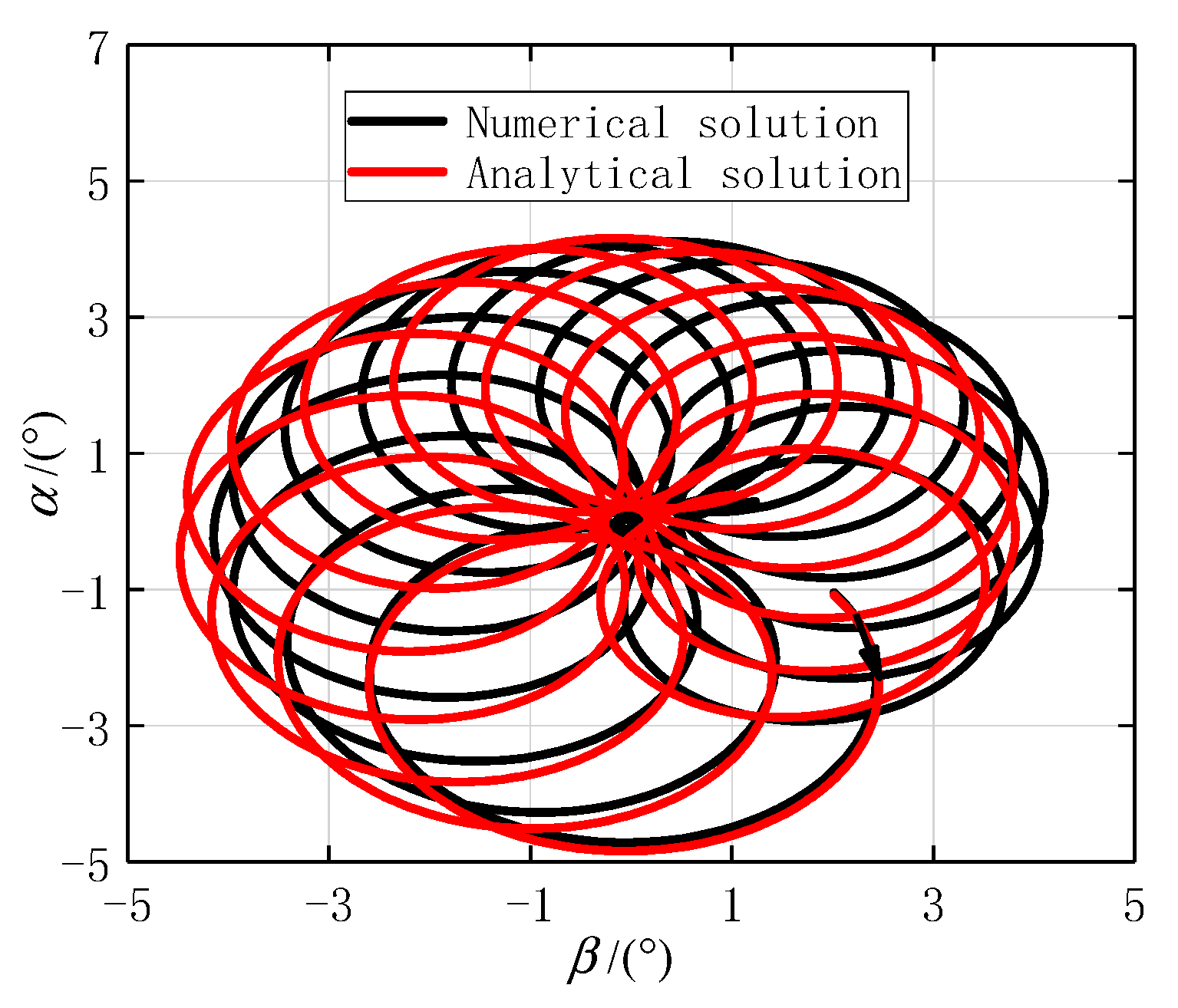
5.3. Numerical and Analytical Solutions at the Second Stage

The angular motion of the projectile at the second stage is shown in Figure 8. Based on Equation (50), the angular motion of the projectile should be a bicircular motion with two decreasing amplitudes at this stage. The angular frequencies and damping indices that were calculated by the two methods are approximately the same. However, their respective convergence centers were different. The convergence center of the analytical solution was $(-0.102°,0)$, while the convergence center of the numerical solution was $(0.306°,0)$. Due to gravitational effects which were neglected in the analytical solution, the AOS was non-zero value that increased with time. When the impulse action was over, the AOS converged to the dynamic equilibrium angle. As such, the angular motion curve of the numerical solution is to the right of that of the analytical solution.

The relationship between $\beta$ and ${\psi }_{\mathrm{d}}$ that was obtained by the numerical method is depicted in Figure 9. When $\beta$ was greater than zero, ${\psi }_{\mathrm{d}}$ increased. When $\beta$ was less than zero, ${\psi }_{\mathrm{d}}$ decreased. This observation explains how the aerodynamic angle of attack affects the velocity direction.

Three types of ${\psi }_{\mathrm{d}}$ at the second stage are shown in Figure 10. Since the AOS caused by gravity was positive and increased over time, the numerical solution ${\psi }_{\mathrm{d}}$ increased. As such, the difference between the two methods increased. The analytical solution ${\psi }_{\mathrm{d}}$ converged to a negative analytical average value, which was obtained according to Equation (57). Although the initial $\beta$ that was caused mainly by the impulse force was positive, it rapidly became negative due to the bicircular motion. Since the convergence center of $\beta$ was negative, the average value of ${\psi }_{\mathrm{d}}$ was also negative.

The value of ${\psi }_{\mathrm{d}}$ that was obtained by the numerical method for the two stages was −0.1555 degrees, while the one obtained by the analytical method was −0.1591 degrees. This indicates that both analytical and numerical solutions are in good agreement. It can be concluded that analytical equations can be used for the control system to predict the velocity direction of the projectile.

The value of ${\psi }_{\mathrm{d}}$ at the first stage was −0.0961 degrees and −0.0594 degrees at the second stage. That meant that the impulse action and the aerodynamic action both changed the velocity in the same direction, and the impulse effect was 1.6 times greater than the aerodynamic effect. If the impulse jets were mounted in front of the center of mass of spin-stabilized projectiles, the initial value of $\beta$ at the second stage would be negative. However, the convergence center of $\beta$ was positive, thus ensuring a positive average value of ${\psi }_{\mathrm{d}}$. The impulse action and the aerodynamic action change the velocity in opposite directions. The correction ability of an impulse jet is thus weakened.

6. Conclusions

In this paper, a derivation procedure for a new 155-mm lateral impulse correction dual-spin projectile is presented. A fully nonlinear 7-DOF dynamic model with linear angular motion equations and velocity deflection angle equations is provided. Movement characteristics of the projectile that was subjected to a lateral impulse are addressed by both numerical and analytical methods. The physical law of a lateral impulse correcting projectile trajectory is explained in detail. Furthermore, the equation for the velocity deflection angle is obtained, which can be used for the control system.

In future work, the relationship between the impact point and the velocity deflection angle will be investigated. Lastly, the design of the control system that is based on the impact point prediction will be addressed.

References

1. Yang, Z.W.; Wang, L.M.; Zhong, Y.W. Calculation method for the nonlinear angular motion attraction domain of spin-stabilized projectile. Acta Armamentarii 2021, 42, 1195–1203. [Google Scholar]
2. Costello, M.; Peterson, A. Linear theory of a dual-spin projectile in atmospheric flight. J. Guid. Control Dyn. 2000, 23, 789–797. [Google Scholar] [CrossRef]
3. Hainz, L.C.; Costello, M. Modified projectile linear theory for rapid trajectory prediction. J. Guid. Control Dyn. 2005, 28, 1006–1014. [Google Scholar] [CrossRef]
4. Theodoulis, S.; Morel, Y.; Werbert, P. Trajectory-based accurate linearization of the 155 mm spin-stabilized projectile dynamics. In Proceedings of the AIAA Modeling and Simulation Technologies Conference, Chicago, IL, USA, 10–13 August 2009; pp. 1–21. [Google Scholar]
5. Li, J.; He, G.; Guo, H. A study on the aerodynamic characteristics for a two-dimensional trajectory correction fuze. Appl. Mech. Mater. 2015, 703, 370–375. [Google Scholar] [CrossRef]
6. Liang, K.; Huang, Z.; Zhang, J. Optimal design of the aerodynamic parameters for a supersonic two-dimensional guided artillery projectile. Def. Technol. 2017, 13, 206–211. [Google Scholar] [CrossRef]
7. Liu, X.; Wu, X.; Yin, J. Aerodynamic characteristics of a dual-spin projectile with canards. Proc. Inst. Mech. Eng. Part G J. Aerosp. Eng. 2019, 233, 4541–4553. [Google Scholar] [CrossRef]
8. Wernert, P.; Theodoulis, S. Modelling and stability analysis for a class of 155 mm spin-stabilized projectiles with course correction fuse (CCF). In Proceedings of the AIAA Atmospheric Flight Mechanics Conference, Portland, OR, USA, 8–11 August 2011; pp. 1–14. [Google Scholar]
9. Wang, Z.G.; Li, W. Analysis of free motion characteristics for dual-spin projectile. Appl. Mech. Mater. 2013, 427, 69–72. [Google Scholar] [CrossRef]
10. Chang, S.J.; Wang, Z.Y.; Liu, T.Z. Analysis of spin-rate property for dual-spin-stabilized projectiles with canards. J. Spacecr. Rockets 2014, 51, 958–966. [Google Scholar] [CrossRef]
11. Chang, S.J. Dynamic Response to canard control and gravity for a dual-spin projectile. J. Spacecr. Rockets 2016, 53, 558–566. [Google Scholar] [CrossRef]
12. Gagnon, E.; Vachon, A. Efficiency analysis of canards-based course correction fuze for a 155-mm spin-stabilized projectile. J. Aerosp. Eng. 2016, 29, 04016055. [Google Scholar] [CrossRef]
13. Spagni, J.; Theodoulis, S.; Wernert, P. Flight control for a class of 155 mm spin-stabilized projectile with reciprocating canards. In Proceedings of the AIAA Guidance, Navigation, and Control Conference, Minneapolis, MN, USA, 13–16 August 2012; pp. 1–8. [Google Scholar]
14. Theodoulis, S.; Gassmann, V.; Wernert, P. Guidance and control design for a class of spin-stabilized fin-controlled projectiles. J. Guid. Control Dyn. 2013, 36, 517–531. [Google Scholar] [CrossRef]
15. Theodoulis, S.; Seve, F.; Wernert, P. Robust gain-scheduled autopilot design for spin-stabilized projectiles with a course-correction fuze. Aerosp. Sci. Technol. 2015, 42, 477–489. [Google Scholar] [CrossRef]
16. Thurman, S.W.; Flashner, H. Robust digital autopilot design for spacecraft equipped with pulse-operated thrusters. J. Guid. Control Dyn. 1996, 19, 1047–1055. [Google Scholar] [CrossRef]
17. Zimpfer, D.J.; Shieh, L.S.; Sunkel, J.W. Digitally redesigned pulse-width modulation spacecraft control. J. Guid. Control Dyn. 1998, 21, 529–534. [Google Scholar] [CrossRef]
18. Guidos, B.J.; Cooper, G.R. Linearized motion of a fin-stabilized projectile subjected to a lateral impulse. J. Spacecr. Rockets 2002, 39, 384–391. [Google Scholar] [CrossRef]
19. Burchett, B.; Costello, M. Model predictive lateral pulse jet control of an atmospheric rocket. J. Guid. Control Dyn. 2002, 25, 860–867. [Google Scholar] [CrossRef]
20. Corriveau, D.; Wey, P.; Berner, C. Thrusters pairing guidelines for trajectory corrections of projectiles. J. Guid. Control Dyn. 2011, 34, 1120–1128. [Google Scholar] [CrossRef]
21. Bojan, P.; Milos, P.; Danilo, C. Frequency-modulated pulse-jet control of an artillery rocket. J. Spacecr. Rockets 2012, 49, 286–294. [Google Scholar]
22. Glebocki, R.; Jacewicz, M. Parametric study of guidance of a 160-mm projectile steered with lateral thrusters. Aerospace 2020, 7, 61. [Google Scholar] [CrossRef]
23. Lee, J.; Min, B.; Byun, Y. Computational investigation and design optimization of a lateral-jet-controlled missile. J. Aircr. 2006, 43, 1292–1300. [Google Scholar] [CrossRef]
24. Liu, L.J.; Zhu, C.H.; Yu, Z. Guidance and ignition control of lateral-jet-controlled interceptor missiles. J. Guid. Control Dyn. 2015, 38, 2455–2460. [Google Scholar] [CrossRef]
25. Glebocki, R.; Jacewicz, M. Sensitivity analysis and flight tests results for a vertical cold launch missile system. Aerospace 2020, 7, 168. [Google Scholar] [CrossRef]
26. McCoy, R.L. Modern Exterior Ballistics, 2nd ed.; Schiffer Publishing Ltd.: Atglen, PA, USA, 1999; pp. 187–188. [Google Scholar]
27. Han, Z.P. Exterior Ballistics of Projectiles and Rockets, 2nd ed.; Beijing Institute of Technology Press: Beijing, China, 2008; pp. 174–176. [Google Scholar]
Figure 1. The overall structure of a dual-spin projectile.
Aerospace 08 00309 g001
Figure 2. Two reference frames of a dual-spin projectile. (a) the ground reference frame, (b) the no-roll reference frame.
Aerospace 08 00309 g002
Figure 3. Parameters in the complex plane. (a) total AOA in the complex plane, (b) velocity deflection angle in the complex plane.
Aerospace 08 00309 g003
Figure 4. Two entire trajectories: one is a normal trajectory without control, and the other one is a correction trajectory with a single impulse jet being ignited. (a) altitude vs. range, (b) crossrange vs. range.
Aerospace 08 00309 g004
Figure 5. The spin rate of two bodies.
Aerospace 08 00309 g005
Figure 6. Angular motion at the first stage.
Aerospace 08 00309 g006
Figure 7. Velocity deflection angle at the first stage.
Aerospace 08 00309 g007
Figure 8. Angular motion at the second stage.
Aerospace 08 00309 g008
Figure 9. Relationship between β and ψ d .
Aerospace 08 00309 g009
Figure 10. ψ d vs. time at the second stage.
Aerospace 08 00309 g010