Article

Deep Neural Network Feature Selection Approaches for Data-Driven Prognostic Model of Aircraft Engines

Industrial and Manufacturing Engineering, North Dakota State University, Fargo, ND 58102, USA
*
Author to whom correspondence should be addressed.
Aerospace 2020, 7(9), 132; https://doi.org/10.3390/aerospace7090132
Submission received: 29 July 2020 / Revised: 28 August 2020 / Accepted: 3 September 2020 / Published: 4 September 2020
(This article belongs to the Special Issue Fault Detection and Prognostics in Aerospace Engineering)

Abstract

:
Predicting Remaining Useful Life (RUL) of systems has played an important role in various fields of reliability engineering analysis, including in aircraft engines. RUL prediction is critically an important part of Prognostics and Health Management (PHM), which is the reliability science that is aimed at increasing the reliability of the system and, in turn, reducing the maintenance cost. The majority of the PHM models proposed during the past few years have shown a significant increase in the amount of data-driven deployments. While more complex data-driven models are often associated with higher accuracy, there is a corresponding need to reduce model complexity. One possible way to reduce the complexity of the model is to use the features (attributes or variables) selection and dimensionality reduction methods prior to the model training process. In this work, the effectiveness of multiple filter and wrapper feature selection methods (correlation analysis, relief forward/backward selection, and others), along with Principal Component Analysis (PCA) as a dimensionality reduction method, was investigated. A basis algorithm of deep learning, Feedforward Artificial Neural Network (FFNN), was used as a benchmark modeling algorithm. All those approaches can also be applied to the prognostics of an aircraft gas turbine engines. In this paper, the aircraft gas turbine engines data from NASA Ames prognostics data repository was used to test the effectiveness of the filter and wrapper feature selection methods not only for the vanilla FFNN model but also for Deep Neural Network (DNN) model. The findings show that applying feature selection methods helps to improve overall model accuracy and significantly reduced the complexity of the models.

1. Introduction

Modern computational capability has become more powerful over the past decades. This has induced a new trend of employing various data-driven models in many fields. Despite the fact that modern computers can complete complex tasks, researchers are still searching for solutions to reduce the computational time and complexity of the data-driven models to increase the likelihood that the models can be employed in real-time operation.
The same challenge has also applied to a certain type of aerospace data, which in this case, is the estimation of Remaining Useful Life (RUL) of the aircraft gas turbine engines. The main purpose of this work is to prove the theory that a particular group or a set of prognostics features (attributes or variables) from the aircraft gas turbine engines data can be selected prior to the training phase of Artificial Neural Network (ANN) modeling in order to reduce the complexity of the model. The same assumption also is believed to be applicable to the Deep Neural Network (DNN) model. It might also be applied to other complex deep learning models, i.e., Convolutional Neural Network (CNN), Recurrent Neural Network (RNN), and their variations as well.
In order to validate the aforementioned theory, the prognostics of aircraft gas turbine engines dataset or Commercial Modular Aero-Propulsion System Simulation (C-MAPSS) dataset derived from NASA Ames Prognostics Center of Excellence (PCoE) [1] was used to develop preliminary vanilla ANN models with selected features from different feature selection methods. Furthermore, to prove that similar assumptions can also be deployed to other deep learning algorithms, the Deep Neural Network or DNN models have also been developed based on some selected features derived from the ANN validation models. The final goal was to determine which feature selection method was the most suitable for the deep learning model in general to predict prognostics state or Remaining Useful Life for aircraft gas turbine engines data. End results from various future selection methods were compared against the one that is using original features. The ANN and DNN models with selected features were studied and compared based on their performance.
Based on the aforementioned goal, the summary of the main contributions of this work are:
  • Extract meaningful features for neural network-based and deep learning data-driven models from the C-MAPSS dataset.
  • Suggest the novel neural network-based feature selection method for aircraft gas turbine engines RUL prediction.
  • Develop deep neural network models from selected features.
  • Show how the developed methodology can improve the RUL prediction model by comparing its performance/error and complexity to the model derived from original features.

1.1. Neural Network for RUL Prediction

Prognostic and Health Management (PHM) is aimed at improving reliability and reducing the cost of maintenance of the system’s elements [2]. Remaining Useful Life (RUL) in PHM is defined as the amount of time left before systems or elements cannot perform as their intended function. Therefore, RUL prognostics are used to evaluate the equipment’s life status in order to plan future maintenance [3]. With enough condition monitoring data, data-driven machine learning methods can be used to learn the degradation patterns directly from data in order to generate predictive prognostics models. Data-driven model using machine learning has an advantage over physics-based [4] and traditional data-driven statistical-based models [5]. For example, machine learning models can be implemented without prior degradation knowledge [6]. Neural network algorithms have particularly been receiving more attention compared to other machine learning algorithms as they have outperformed other algorithms as well as their ability to approximate high dimensional non-linear regression function directly from raw data [7].
The Artificial Neural Networks (ANN) model is fundamentally based on biological neural networks. Sigmoid functions are applied to the nodes of ANN to connect and sum the total weights of the neural network. A sigmoid function is a Gaussian spheroid function, which can be expressed as:
Y ( x ) = e ( | | X c | | 2 2 σ 2 )
The hidden neurons in ANN measure the distance between the input vector x and the centroid c from the data cluster. The measured values are the output of the ANN. In Equation (1), the σ parameter represents the radius of the hypersphere determined by iteratively selecting the optimum width. The weights of the neural network are updated at the neural nodes using error back-propagation, which is a stochastic gradient descent technique. Then the weights of each individual neural node are fed forward to the next layer. This technique is often referred to as Feedforward Neural Network (FFNN). This is how ANN “learns” the data pattern through its weights [8].
In 2006, Geoffrey Hinton suggested the early design of deep learning algorithms based on the aforementioned FFNN [9]. The vanilla FFNN generally consists of only the hidden layer with a sigmoid activation function described in Equation (1). Multiple configurations of deep learning algorithms, such as Deep Neural Network (DNN), Convolutional Neural Network (CNN), Recurrent Neural Network (RNN), etc., have been widely used as data-driven modeling algorithms. Most of them have outperformed every other well-known data-driven algorithms in the past.
One aspect to keep in mind before employing any deep learning algorithm is that each deep learning algorithm might be suitable for different tasks. This heavily depends upon the different data characteristics and type of target models. The deep learning algorithms also include different types of activation functions and optimizers. These are the key differences between deep learning algorithms and vanilla ANN or FFNN that have been proposed in the early years [10].
In this work, we only employed DNN with auto-encoder as a modeling algorithm. All encoded and decoded processes happen inside the hidden layers of the network through parameterized function [9,10]. The construction of DNN with auto-encoder is briefly illustrated in Figure 1. Unlike the ANN that uses sigmoid function as an activation function, our DNN layers used Rectified Linear Units (ReLU) as activation function. The ReLu function can be simply expressed as:
f ( x ) = x + = max ( 0 , x )
where x is the input to a neuron and + represents the positive part of its arguments. The ReLU function has been demonstrated to achieve better general regression tasks training for deeper networks compared to other activation functions such as the logistic sigmoid and the hyperbolic tangent (tanh) [10]. Therefore, the ReLU function has been chosen to use for modeling Remaining Useful Life (RUL) prediction for our PHM data while the ANN with sigmoid function has been used as a validation algorithm for feature selection methods.
The estimation of the RUL or “health state” of a system or its components is one of the main tasks for prognostics analysis. The RUL estimations often involve the prediction of the life span based on time or cycles, which is also known as the regression task. In PHM, the RUL is determined using the historical data collected from the system’s sensors or signals. The ANN-based or deep learning data-driven models have been proven to work relatively well with these types of PHM tasks [11]. However, one of the challenges is to reduce the complexity of the neural network prior to the training states. This might possibly be done by reducing the input training data. One possible way that can help in reducing the complexity of the model is to select only meaningful features or attributes from the raw dataset before model training.

1.2. Related Works

Multiple deep learning algorithms have been used to generate data-driven models to predict RUL for C-MAPSS aircraft gas turbine engines data. It can be observed from the literatures [12,13,14,15,16,17,18,19,20] that the most suitable deep learning algorithms for training the high accuracy C-MAPSS models is the Long-Short Term Memory Recurrent Neural Network (LSTM). The hybrid deep neural network layers with LSTM is also an ongoing investigation and experiment on the C-MAPSS dataset. This approach believes to achieve the higher accuracy among other algorithms that have been employed. The most important drawback of the hybrid models is the high complexity of the model architectures. These models can also have limitless variations and architecture structures. It is best to reduce the complexity of the model as much as possible and one way to achieve that is to limit the number of input nodes. This is the area that feature selection methods can be brought in.
There are many publications on applying ANN-based or deep learning algorithms to C-MAPSS aircraft gas turbine engines data. However, all previous works have never introduced the feature selection approaches into their model architectures. Also, the usefulness of any particular feature selection methods have not been addressed in any prior works.
The next paragraph concludes the contribution of past publications for such an approach. We specifically only included the works that employed deep neural network algorithms for prognostics of C-MAPSS aircraft gas turbine engines data modeling here. It might be worth to note that there are other research works that used other data-driven algorithms or machine learning algorithms, which are not mentioned here.
Chen Xiongzi, et al., (2011) conducted a comprehensive survey of the three main data-driven methods for aircraft gas turbine engines, namely particle filtering methods, neural network, and relevant vector machine methods [12]. Mei Yuan, et al., (2016) applied RNN network methods for fault diagnosis and estimation of remaining useful life of engines [13]. Faisal Khan, et al., (2018) used particle filter algorithms to generate the arbitrary input data points before training their models with neural networks. Unlike, vanilla neural network algorithm, their models employed radial basic function (RBF) as activation function instead of original sigmoid function [14]. Xiang Li, et al., (2018) applied the Convolutional Neural Network (CNN) as a time window approach to generate a feature extraction model of engine data [15]. Ansi Zhang et al., (2018) proposed a supervised domain adaptation approach by exploiting labeled data from the target domain aims to fine-tune a bi-directional Long-Short Term Memory Recurrent Neural Network (LSTM) previously trained on the source domain [16]. Zhengmin Kong et al., (2019) also very recently developed the models based on CNN. They employed CNN as part of the network layers in their experiment and proposed the hybrid models by combining the CNN layers with LSTM layers. Their approaches have proven to achieve highest accuracy over the other standard methods [17]. Other works previously published [18,19,20] mostly focused on adopting the LSTM network and proposing new models without addressing the complexity reduction in their approaches. While each work proposed the different network architectures and the performances of the models have been improved over time, what they failed to address is whether the complexity reduction in ANN-based models can play a role in improving the complexity of the model. This work aims to address the issue of a selection approach to reduce learning times.
The rest of the paper is organized as follows: Section 2 covers the methodology outlining all methods and approaches used for the defined problem. Section 3 describes the experimental setup with detail of data description and comparing final results from all models. Section 4 discusses and compares results from all modela. Lastly, a final conclusion and possible future works highlight are discussed in Section 5.

2. Methodology

In this section, all essential details of auto-encoder deep neural network used in our experiment will be discussed. The problem definition, and all notations will also be clearly defined, as well as the illustration of how our proposed deep neural network architecture can be applied for RUL aircraft gas turbine engines prediction with feature selection and neural network modeling framework.

2.1. Problem Definition

Starting with the raw data, which is denoted as, D S = { ( x S i ,   y S i ) } i = 1 N s , the data contains N s training sample where x S i X S is a feature with a length of T i and q S is the number of features, in which, x S i = = { x t i } t = 1 T i   R q S × T i . In addition, y S i Y S is denoted as Remaining Useful Life (RUL) also with the length T i (feature space and RUL space are within the same length) with y S i = { 𝓎 t i } t = 1 T i   0 T i . where t { 1 ,   2 ,   ,   T i } , x t i q S , and 𝓎 t i   0 , represent the t -th measurement of all variables and RUL label, respectively. Similarly, the estimated target domain, D T =   { x T i } i = 1 N T   where x T i   X T and X T q T × T i with no labels. The source and target domain, D S   and D T , are assumed to possibly have a different probability distribution, P ( X S ) P ( X T ) . The primary goal is to define a function g that can derive or learn from the source data that can approximate the corresponding RUL for the target domain at the testing time, such, y T i   g ( x T i ) , with the preliminary assumption that mapping between input ( x ) and output ( y ) is somehow similar across all domains.

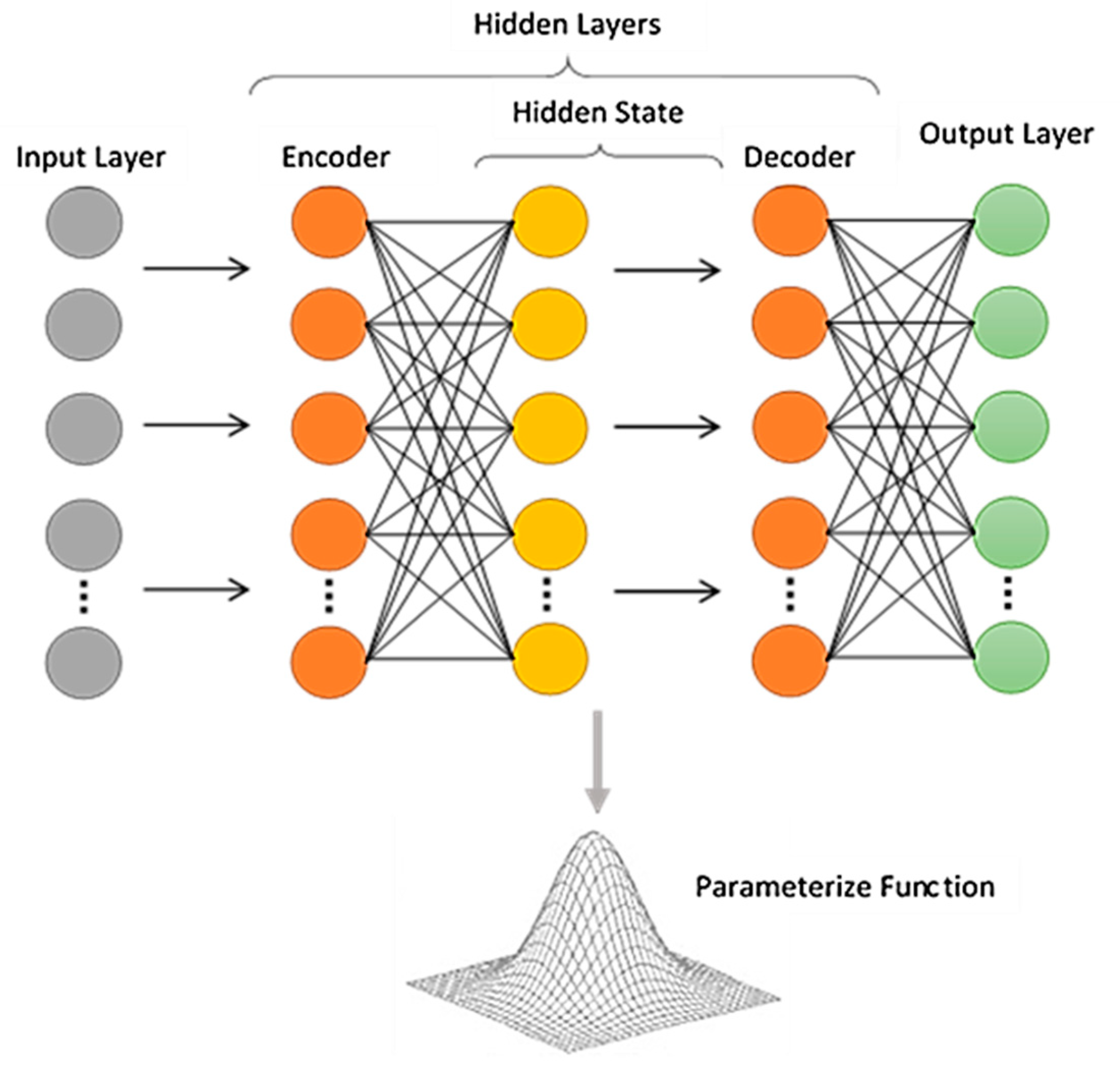
2.2. Deep Neural Network Architecture

While there are existing deep learning algorithms that have been proposed to accommodate for PHM of aircraft gas turbine engines data modeling [12,13,14,15,16,17,18,19,20], this work focuses on using a deep neural network with auto-encoder with a specific use case and specifications that fit into problem definition previously identified.
The DNN used in this work focused on the feedforward architecture by the H2O package in Python API [21]. H2O is based on multi-layer feedforward neural networks for predictive modeling [22]. The following are some of the H2O DNN features used for this experiment.
  • Supervised training protocol for regression tasks
  • A multi-threaded and distributed parallel computation that can be run on a single or a multi-node cluster
  • Automatic, per-neuron, adaptive learning rate for fast convergence
  • Optional specification of the learning rate, annealing, and momentum options
  • Regularization options to prevent model overfitting
  • Elegant and intuitive web interface (Flow)
  • Grid search for hyperparameter optimization and model selection
  • Automatic early stopping based on the convergence of user-specified metric to a user-specified tolerance
  • Model check-pointing for reduced run times and model tuning
  • Automatic pre- and post-processing for categorical numerical data
  • Additional expert parameters for model tuning
  • Deep auto-encoders for unsupervised feature learning.
In the proposed DNN model, deep neural network layers are used to extract the temporal features from the time length, T i . The hidden state units of the neural consist of, the hidden state vector h t 1 h , input vector (as defined in problem definition), x t i R q , and the activation function, f . All operations in DNN layers can be written as:
i t = f ( W t x t i + W t h t 1 + b i )
o t = f ( W o x t i + W o h t 1 + b o )
where i and o represent input and output states. W and W are matrices of updated weights and weights from the hidden state, and b is the bias vector.
Unlike in vanilla ANN, in the proposed DNN, the activation function f is the Rectifier Linear function [23] instead of the sigmoid function. The DNN activation function can be represented as;
f ( α ) = max ( 0 ,   α )     +
where, in this case, α represent the state functions (Equations (3) and (4)) that firing into the input neural.
Another important aspect of the DNN model architecture is the loss function, denoted by, . For this work, the Huber loss function was selected because it [24] has proven to work best in terms of accurately projecting the RUL, y S i Y S , of the source domain, D S . The Huber loss function can be described as;
y i ( θ f ,   θ y ) = { 1 2 | | 𝓎 ^ t i 𝓎 t i | | 2 2 ,                 f o r   | | 𝓎 ^ t i 𝓎 t i | | 1 1   | | 𝓎 ^ t i 𝓎 t i | | 1 1 2 ,       O t h e r w i s e
where, θ f is the space representation of the target input that mapped through the feature extraction layers into a new space. In addition, θ y is the domain regression space generated by logistic repressor [24], and, 𝓎 ^ t i is RUL prediction from the source domain.
The objective in training DNN is to minimize the prediction loss, y i , which can be described by;
min θ f , θ y [ 1 N s i = 1 N s y i ( θ f ,   θ y ) ]
The DNN model used in this work is depicted in Figure 2. This DNN model architecture is trained to predict for each input, x i , real value y i and its domain label d i for the source domain and only domain label for the target domain. The first part of the DNN architecture is the feature extractor, g f , that decomposes the inputs and maps them into the hidden state, h t 1 h . The model then embeds the output space as a feature space f of the deeper layers and repeats this process as needed. As previously detailed, this vector space parameter that is the result of feature mapping is, θ f i.e., f = g f ( θ f ) . This feature space f is first mapped to a real-value 𝓎 t i variable by the function, g y ( f ; θ y ) , which is composed of fully-connected neural network layers with parameter, θ y . The dropout layer with a rate of 0.4 was applied to avoid the overfitting issue [25].
Another goal is to find the feature space that is domain invariant, i.e., finding a feature space f in which P ( X S ) and P ( X T ) are similar. This is one of the challenges in training, which can be improved by applying the “feature selection” prior to training (detailed in the further section). Another objective is to minimize the weights of feature extractor in the direction of the regression loss, y i . In more detail, the model loss function can be used to derive the final learning function, g , through parameter θ , which means the RUL prediction result (described in Equation (6)), 𝓎 ^ t i = g y ( g f ( θ f ) ; θ y ) .
The way the DNN algorithm update its learning weights, θ , is through the gradient descent update [26] in the form of;
θ f   θ f   λ ( y i θ f )
θ y   θ y   λ ( y i θ y )
Usually, the Stochastic Continuous Greedy (SCG) estimate is used to update the Equations (8) and (9). The learning rate, λ , represents the learning steps taken by the SCG as training processes.

2.3. Feature Selection Methods for Neural Network Architectures

In prognostic applications, feature extraction occurs after receiving raw data from sensors. The feature extraction usually involves signal processing and analysis in the time or frequency domain. The purpose is to transform raw signals into more informative data that well-represents the system [27]. In other words, feature extraction is the process of translating sensor signals into data. In contrast, the purpose of feature selection is to select a particular set of features in the dataset that is believed to be more relevant for modeling. These feature selection processes always execute after the feature extraction and occur in between pre-processing and the training or pre-training phase of the data modeling framework.
Three common feature selection strategies have been discussed in the literature: (1) filter approach, (2) wrapper approach, and (3) embedded approach. This paper will only discuss the filter and wrapper approaches. Figure 3 shows the processes flow and role difference role of feature extraction and feature selection in the data modeling process.
Filter methods employ statistical, correlation, and information theory to identify the importance of the features. The performance measurement metrics of filter methods usually use the local criteria that do not directly relate to model performance [28].
There are currently multiple baseline filter methods popularly employed for feature selection processes. However, the result from the experiments showed that only the correlation-based methods were suitable for the case study data. This is due to the fact that correlation-based methods evaluate the feature with a direct correlation to the target variable. In other words, the correlation-based filter methods make selections based on the modeling objectives, which can imply that these methods are more suitable to the data with the target variable. The correlation-based filter methods included in this work is Pearson correlation [29,30]. Additionally, the result from other statistical-based methods, namely Relief algorithm, Deviation selection, SVM selection, and PCA selection [31], was also included to provide a complete comparison.
Wrapper methods use a data-driven algorithm that performs the modeling for the dataset to select the set of features that yield the highest modeling performance [32]. Wrapper methods are typically more computationally intensive compared to filter methods. There are four main baseline wrapper methods [32]: (1) forward selection, (2) backward elimination, (3) brute force selection, and (4) evolutionary selection.
Forward selection and backward elimination are search algorithms with different starting and stopping conditions. The forward selection starts with an empty selection set of features, then adds an attribute in each searching round. Only the attribute that provides the highest increase in performance is retained. Afterwards, another new searching cycle is started with the modified set of selected features. The searching of forward selection stops when the added attribute in the next round does not further improve the model performance.
In contrast, the backward elimination method performs in the reverse process. Backward selection starts with a set of all attributes, and then the searching processes continue to eliminate attributes until the next set of eliminated attributes does not provide any further improvements of modeling performance. The brute force selection method uses search algorithms that try all combinations of attributes. Evolutionary selection employs a genetic algorithm to select the best set of features based on the fittest function measurement [33]. Because of computational and time limitations, the brute force selection could not be included in this experiment. Only forward selection, backward elimination, and evolutionary selection were implemented [34].

2.4. Neural Network Data-Driven Modeling Framework

In general, the modeling framework for this experiment is similar to a data-driven modeling framework that was developed from a cross-industry standard process for data mining (CRISP-DM) [35]. The standard construction consists of five phases: (1) definition states phase, (2) preprocessing phase, (3) training phase, (4) testing phase, and (5) evaluating phase [36]. In addition to the standard construction, the feature engineering phase and pre-training phase might be important prior to the training phase.
The feature engineering phase was introduced in “Features selection procedure for prognostics: An approach based on predictability” [34] and the pre-training phase was introduced in “The difficulty of training deep architectures and the effect of unsupervised pre-training” [37] to overcome issues in training deep learning models, while it also helped to improve some aspects of model performance. The details of these two additional phases have also been detailed by others [34,37].
As mentioned in Section 2.1, one of the challenges of training the deep learning model is to seek for a feature space f in which P ( X S ) and P ( X T ) are similar. Selecting only the meaningful feature is believed to help reduce the dissimilarity in the feature space that effect the predictability of the model. This is also the way to reduce the complexity of the model architecture and might also improve the prediction accuracy of the deep learning models. One possible framework that incorporates the feature engineering phase and pre-training phase into the CRISP-DM standard is illustrated in Figure 4.

3. Experimental Setup and Results

The first part of the experiment was designed to compare the effectiveness of using different feature selection methods and filtering for ANN modeling of the prognostics dataset. The aircraft gas turbine engines dataset with 21 attributes was fed into different filter and wrapper feature selection methods to identify particular sets of features prior to the model training phase. The selected sets of features were then used as training features or training attributes for the ANN model. The second part was to test the feature selected using ANN modeling with the DNN architecture. The results from different sets of features were compared in order to determine the most suitable set of selected features. Finally, the final-best DNN model for predicting RUL of aircraft gas turbine engines was determined.

3.1. C-MAPSS Aircraft Engines Data

Commercial Modular Aero-Propulsion System Simulation (C-MAPSS) is a simulation tool used to generate the turbofan engine degradation run-to-failure test dataset. This test dataset was derived from the NASA Ames prognostics data repository [1]. The C-MAPSS dataset is one of the most popular benchmark datasets used in the prognostics and diagnostics research community. This dataset provides a set of editable input parameters to simulate various operational conditions for aircraft gas turbine engines [38]. The operational conditions include sea-level temperature, Mach number, and altitude. The C-MAPSS dataset includes four sub-datasets described in Table 1.
Each sub-dataset FD001, FD002, FD003, and FD004 contains a number of training engines with run-to-failure information and a number of testing engines with information terminating before failure is observed. As for operating conditions, each dataset can have one or six operational conditions based on altitude (0–42,000 feet), throttle resolver angle (20–100°), and Mach (0–0.84). As for fault mode, each dataset can have one mode or two modes, which are, HPC degradation and Fan degradation.
Sub-dataset FD002 and FD004 are generated with six operational conditions, which are believed to be a better representation of general aircraft gas turbine engines operation compared to FD001 and FD003, which could be generated from only one operational condition. Therefore, either data from FD002 or FD004 can be selected for a complete experiment. In this study, the data from FD002 set were selected as a training dataset. As our current model validation set-up (which will be described in Section 3.2), the wrapper methods required roughly 2 to 3 weeks to complete the run. We also keep the consistency of the amount of data points used in feature selection validations and model trainings–in both ANN feature selection validation and DNN model training. Our experiments have been designed this way in order to clearly demonstrate the effectiveness of the feature selection methods used for neural network-based algorithms.
There are 21 features included in the C-MAPSS dataset for every sub-dataset. These attributes represent the sensor signals from the different parts of the aircraft gas turbine engines, as illustrated in Figure 5 [39]. Short descriptions of the features and the plots of all 21 sensor signals of sub-dataset FD002 are illustrated in Figure 6.
It has been suggested by multiple literature references to normalize the raw signal before performing modeling and analysis [13,14,15]. Figure 7 shows the data signals before and after applying z-normalization:
x ˜ t i j = x t i j min ( x j ) max ( x j ) min ( x j )
where, x t i j denotes the original i -th data point of j -th feature at time t and x j is the vector of all inputs of the j -th feature. Each attribute value was normalized individually and scaled down to the same range across all data points.
From the dataset, aircraft gas turbine engines start with various initial wear levels, but all are considered to be at “healthy state” at the start of each record. The engines begin to degrade at a point in time at higher operation cycles until they can no longer function normally. This is considered as the time when the engine system is being at the “unhealthy state”. The training datasets have been collected over the time of run-to-failure information to cover entire life until the engines fail.
It is also reasonable to estimate RUL as a constant value when the engines operate in normal conditions [38]. Therefore, a piece-wise linear degradation model can be used to define the observed RUL value in the training datasets. That is, after an initial period with constant RUL values, it can be assumed that the RUL targets decrease linearly.
Figure 8 illustrates the RUL curves of all unseen or test datasets containing testing engines from FD002 and FD004 dataset. Figure 9 show the example of RUL curves from one degradation engine from FD002 and FD004 dataset. The same degradation behavior is also applied to the training set. These RUL curves represent the health state or prognostic of the aircraft gas turbine engines over cycles until the end-of-life, or the point that the aircraft gas turbine engines can no longer operate normally.
The degradation behavior of the aircraft gas turbine engines can be observed clearer from Figure 9. We presume that the RUL is a constant cycle until it gets to the critical point when the performance of the engine starts to degrade. In the degradation phase, the RUL is represented by a linear function. Hence, the entire RUL curve is identified as a piece-wise linear degradation function. The critical point, Rth, is the point where the aircraft engines started to degrade. The critical points of the aircraft gas turbine engines were predefined based on the condition described by the data source–NASA Ames prognostics data repository [1].
To measure and evaluate the performance of the models with selected features, root mean square error (RMSE) and the scoring algorithm as suggested in [39] were used.
RMSE is commonly used as a performance indicator for regression models. The following is the formula of RMSE:
R M S E = 1 n i = 1 n [ x i x ¯ i ] 2
where, n is the number of prediction datasets, x i is the real value, and x ¯ i is the prediction value. In this case, the x parameters refer to the data points in RUL curve while x i is the actual RUL value and x ¯ i is the RUL value predicted by our models.
The scoring algorithm is as described in the formula below:
s = { i = 1 n e ( d a 1 ) 1     f o r   d < 0 i = 1 n e ( d a 2 ) 1     f o r   d 0
where, s is the computed score, n is number of units under test (UTT), d = t ^ R U L t ^ R U L or Estimated RUL—True RUL, while a 1 = 10 and a 2 = 13 . It can also be explained that the difference between a i is the difference between predicted and observed RUL values and s is summed over all examples. From the formula, the scoring matric penalizes positive errors more than negative errors as these have a higher impact on maintenance policies. Also, note that the lower score means better prediction performance of the model [39].

3.2. Training Procedure and Hyperparameters Selection

For training, the data from input sensors, operational setting, and labeled RUL value from the source data, and only sensors and settings from the target dataset, were used. The raw data were normalized, and the feature selection was applied before the start of all models training. For the training process, the training dataset (as a source) from dataset FD002 were used. The FD002 and FD004 test dataset were used to validate the models and calculate prediction errors (RMSE and Score). As for wrapper methods, we used ANN as a validation algorithm. The cross-validation within the FD002 training data was employed for measuring the performance of the wrapper algorithms. The set-up parameters for ANN validation were fine-tuned based on the best model that was derived from complete attributes (21 features) modeling;
  • 5 Folds Cross-Validation
  • 1000 Training cycles
  • 0.001 Learning rate
  • 0.9 Momentum
  • Linear sampling.
For the DNN hyperparameters selection, the model parameters in H2O DNN algorithm varied as described in Table 2. The grid search to identify the range of the learning rate, λ, was performed after fine-tuning the remaining parameters manually. Additionally, the training sample per iteration was set to auto-tuning, and batch size was set to 1 for all variations.
The best-case scenario is the combination of following hyperparameters; Epoch = 5000, Learning rate = 10−8, Momentum = 0.99, L1 = 10−5, L2 = 0, and Max w2 set to infinity. These are all hyperparameters employed in the final DNN model proposed.

3.3. Experimental Setup and Results

All experiments were implemented on an Intel® Core i7 10th generation i7–10510U 4 cores processor with 8 MB Cache, 1.8 GHz clock speed, and up to 4.9 GHz boost speed with 16 GB RAM and Intel® UHD integrated graphic. The DNN architecture was implemented using Python 3.6 with H2O library/package [21]. The experimental results presented in this section will be broken down into three parts: (1) Feature selected using feature selection methods, (2) Results and models from ANN with the selected feature, and (3) Proposed DNN model. All RMSE and all performance measurements of DNN models reported in this paper are the average results from 20 trials.

3.3.1. Feature Selection for Aircraft Engine Dataset

All possible feature selection methods were performed with the C-MAPSS dataset. Filter methods include; Deviation selection, PCA selection, Relief algorithm selection, selection, SVM selection, and Pearson correlation selection. For wrapper methods, only three methods were implemented, which include; forward selection, backward elimination, and evolutionary selection.
Table 3 shows the ranking of attributes based on coefficients and weights calculated from each filter feature selection method. It is important to note that the ranking of the attributes based on different methods is dependent upon the statistical measures or weights obtained from each method.
For the Pearson correlation, the attributes were not selected if the coefficient was less than −0.01 [29,30]. For PCA, the features have been selected based on weight (selected if weight is more than 0.2) and the PCA matrix [31]. For the Relief algorithm, the attributes were not selected if the calculated weight was below zero [31]. For deviation selection, the feature will be selected if the weights are higher than 1 [31]. It is important to note that the weights of the attributes calculated using the Relief algorithm were unacceptably low (less than 10−12) and there were very large gaps between calculated weights. Similar results were observed with other filter selection methods, including the SVM. It was found that by using the filter methods that provided statistically low weight as for selecting features, the models trained from those features were unable to provide usable prediction results.
The following are the features selected based on these two filtering methods. In addition to the feature weights from Pearson correlation selection and PCA selection in Table 3, the Pearson correlation matrix and PCA matrix are also provided in Appendix A and Appendix B.
  • Pearson correlation; 8 attributes: T30, T50, Ne, Ps30, NRc, BPR, farB, and htBleed.
  • Relief algorithm; 2 attributes: P15 and Nf_dmd.
  • SVM selection; 11 attributes: T2, T24, P30, Nf, epr, phi, NRF, Nf_dmd, PCNfR_dmd, W31, and W32.
  • PCA selection; 17 attributes: T2, T24, T30, T50, P2, P15, P30, Nf, Ne, epr, Ps30, phi, farB, htBleed, Nf_dmd, W31, and W32.
  • Deviation selection; 11 attributes: T2, T24, T50, P2, P15, Ne, epr, Ps30, farB, PCNfR_dmd, and W32.
In reference to the wrapper methods, below are the sets of features selected from each method. It is important to note that for the wrapper methods, ANN validation with the modeling set-up, as mentioned in Section 3.2 was used. Figure 10 shows the validation process using ANN for evolutionary selection.
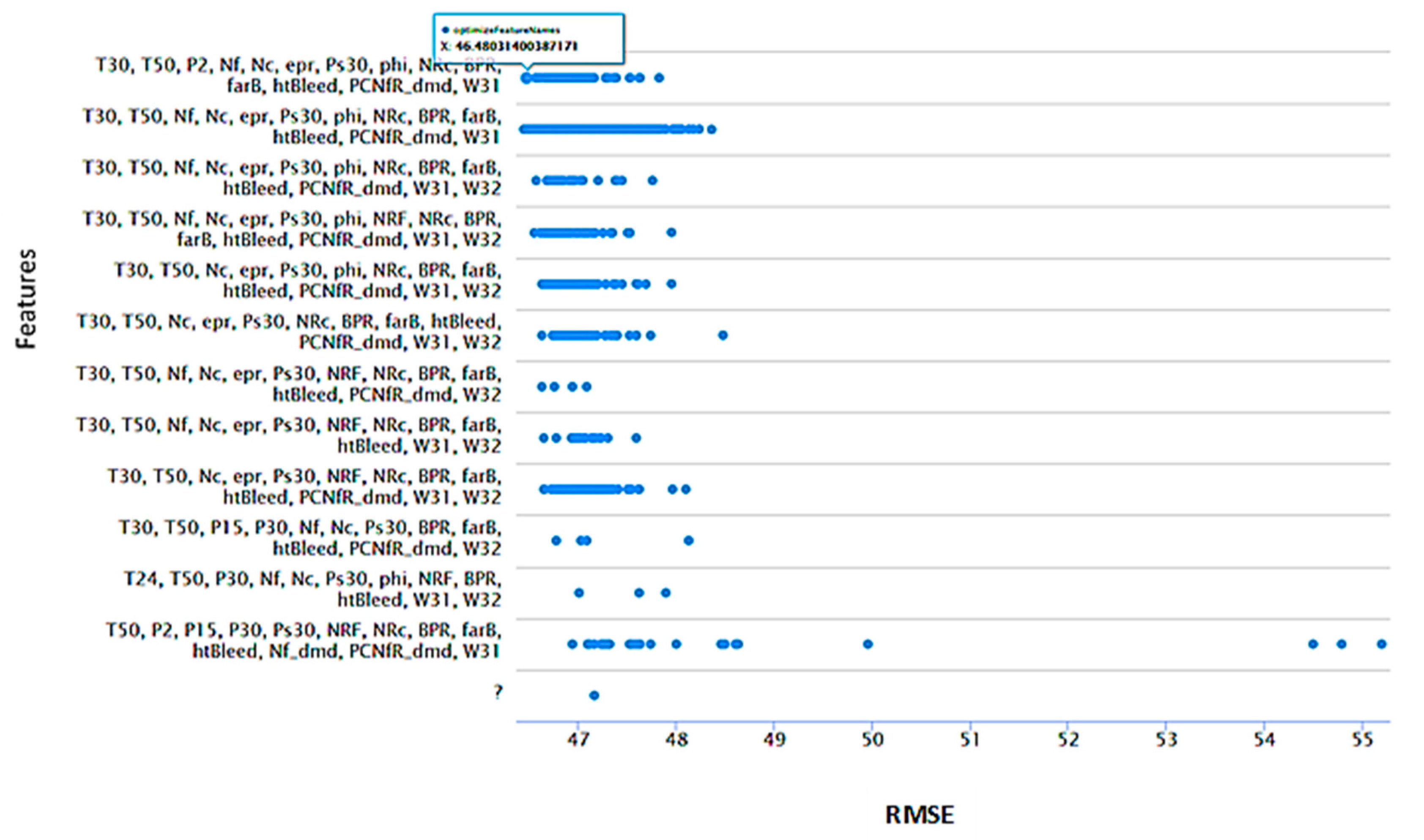
  • Backward elimination; validate RMSE 46.429 from 19 attributes; T2, T30, P2, P15, P30, Nf, epr, Ps30, phi, NRF, NRc, BPR, farB, htBleed, Nf_dmd, PNCfR_dmd, W31, and W32.
  • Evolutionary selection; validate RMSE 46.451 from 14 attributes; T2, T30, T50, P2, Nf, Ne, epr, Ps30, NRc, BPR, farB, htBleed, W31, and W32.
  • Forward selection methods; validate RMSE 46.480 from 11 attributes; T2, T30, T50, P2, P15, Ps30, NRc, BPR, farB, htBleed, and Nf_dmd.
Unlike forward selection and backward elimination methods, which are both based on search algorithms [32], the setting of Evolutionary selection is based on genetic algorithms [40]. However, instead of using fitness function from genetic theory, the evolutionary selection method used ANN validation as fitness measurement. The parameters set-up in our evolutionary selection experiment are; population size = 10, maximum number of generation = 200, using tournament selection with 0.25 size, initial probability for attributes (features) to be switched = 0.5, crossover probability = 0.5 with uniform crossover, and mutation probability = 1 number   of   attributes .
It is also important to note that, in this case, the brute force algorithm was not used. The brute force algorithm is the selection algorithm that can derive the best features set from the data. However, with limited computational capability, it cannot be used in real-time. Therefore, we did not include the Brute force algorithm in this experiment.

3.3.2. DNN Models and Results

Table 4 summarizes RMSE and prediction score results from all DNN models. The complete RUL best fit prediction curves for testing data of all feature selection methods are illustrated in Figure 11 for FD002 test data, and in Figure 12 for FD004 test data, respectively. The blue curves represent the actual RUL from the dataset, and the red lines/dots are the prediction points from our feature selection DNN models. For illustration purposes, Figure 13 and Figure 14 include the prediction curve from one engine of each testing data FD002 and FD004 in order to demonstrate how DNN predicts RUL of one degradation cycle. Additionally, Table 5 includes all DNN models and all prediction error values measured from the DNN models using FD002 test dataset, i.e., absolute error, relative error, relative error lenient, relative error strict, normalized absolute error, root relative squared error, squared error, correlation, squared correlation, prediction average, spearman rho, and Kendall tau. The number of hidden nodes in the DNN layers was identified based on the best models fine-tuned from one-layer ANN models for each feature selection method. We used the same number of hidden nodes from the best ANN models to construct the DNN model layers. Note that we only presented the DNN models from feature selection methods that provided usable prediction results. Therefore, the results from Relief algorithms and SVM selection are not presented here.
Due to the fluctuations in the prediction results from the DNN algorithm, we ran our experiments (training and testing) 100 times for each model. The result from Table 4 are the best prediction results. The fluctuations across 100 iterations for FD002 and FD004 are presented in Figure 15. In addition to the best prediction, we include the mean RMSE and error distributions from the 100 times testing as illustrated in Table 6 and Figure 16. These fluctuations in prediction errors are commonly found in most deep learning algorithms due to the random initial training weights assignment and the amplification effect from the optimizer function in deeper networks. The fluctuations in the prediction result can be more obvious when models are more complex and take a large number of input attributes. We will discuss more on this topic in Section 4.

4. Discussion

As mentioned in the related works (Section 1.2), there have been a number of efforts in developing deep learning models for a C-MAPSS aircraft gas turbine engines dataset [12,13,14,15,16,17,18,19,20]. Currently, the deep learning model with the highest accuracy was proposed by Zhengmin Kong et al. [17]. Their deep learning architecture consists of CNN and LSTM-RNN combined layers and can achieve 16.13 RMSE, while our best Evolutionary DNN model can achieve 44.71 RMSE. This indicates that the performance of our DNN models is poorer than the modern hybrid deep learning models developed in the recent years.
However, to the best of our knowledge, no work has addressed the complexity of the models and the computational burden for model training. All hybrid deep neural network layers are generally overly complex and require exponentially more computational time and resources compared to our proposed Evolutionary DNN. All proposed models in recent years also took all features from the C-MAPSS dataset and disregard the features performance benchmark. Different from those models, our proposed approach applies the feature selection prior to the model training phase to help reduce the number of input attributes, and to improve the model complexity as a result. The reduction in complexity when using less input features is more evident for the high complexity hybrid deep neural network layers.
Additionally, as illustrated in Figure 15 and Figure 16, prediction errors fluctuations can be noticed when training deep learning models. This effect has occurred not only in DNN but also in other types of network layers, such as LSTM-RNN, CNN, and other modern hybrid layers. Based on the results demonstrated in Table 4 and Figure 12, Figure 13, Figure 14, Figure 15 and Figure 16, the key observations of such an effect are as follows:
(1)
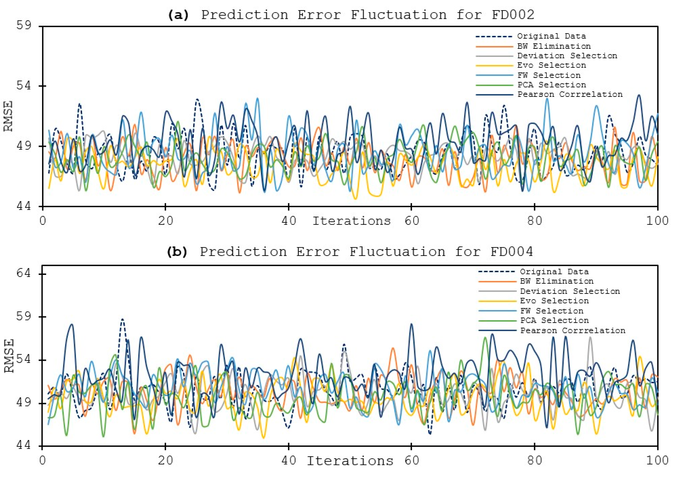
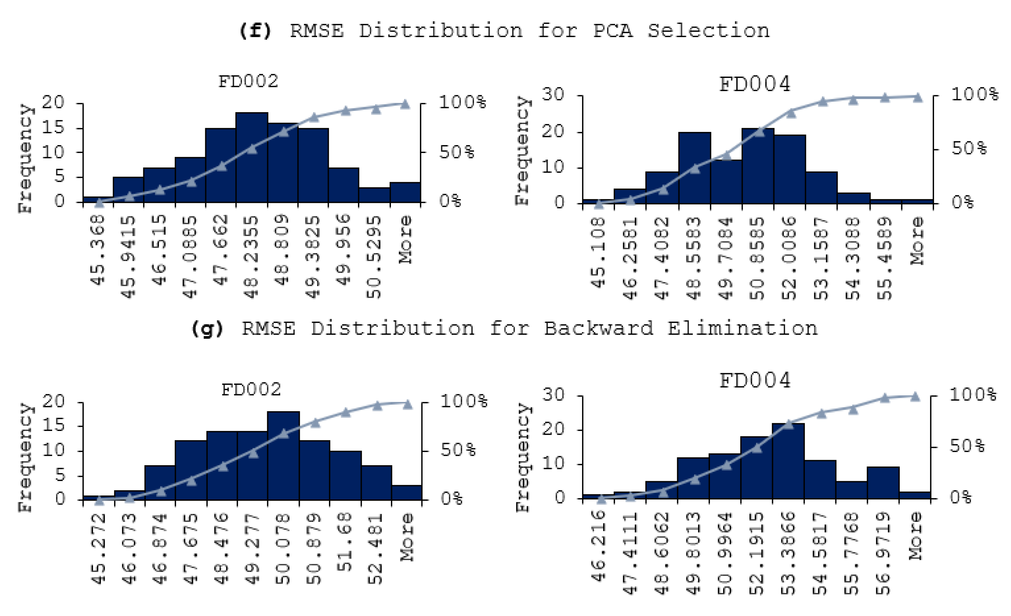
Utilizing fewer features to train the model has shown to lower the error distribution range, compared to using more features. This is due to that the initial random weights assigned to the hidden nodes are smaller when using less feature in model training. In other words, the models are more robust and reliable when using less features. Same observation is also applied for the fluctuation of the prediction errors, in that the prediction results are more stable when using less features in model training.
(2)
In terms of model performance and accuracy, although using selected features does not always guarantee better results, the feature selection methods still help in terms of reducing a computational burden while offering better prediction performance. In our experiment, the Evolutionary selection can achieve both better performance and complexity reduction.
We emphasize that our current goal is not to improve on model performance compared against other existing works; rather, we aim to provide baseline results and demonstrate the significant effect of using feature selections on deep learning models, which have never been addressed before. We believe that the end results can be further improved when applying our feature selection results in the modern hybrid deep neural network architectures.
For our experimental results in general, as mentioned, the best accuracy based on the RMSE results in Table 4 were generated from the Evolutionary method. The complexity of the model has also been significantly improved using a reduced set of features, from 21 attributes to only 14 attributes.
When considering the complexity and computational time, the filter methods were less complex and faster to run because they do not require to train-and-test multiples of ANN model validation in the process. In this study, when performing the selection process, most of the filter methods required only 5–10 min while wrapper methods required 10 h to 10 days to complete.
It is also important to note that the curve fitting and pattern recognition have been vastly improved, as can be seen when comparing the RUL prediction curves in Figure 11, Figure 12, Figure 13 and Figure 14. In greater detail, the DNN model from most of the selected features can reasonably capture the trend of both before and after aircraft gas turbine engines’ degradation intervals.
In summary, our Evolutionary DNN model architecture performs best as a simplified deep neural network data-driven model for C-MAPSS aircraft gas turbine engines data. The feature selection phase (as described in the modeling framework in Figure 4) must be included as a standard in the modeling framework for such a PHM dataset. This is one way to potentially improve the overall performance for RUL prediction for the prognostics of aircraft gas turbine engines data as well as other prognostic datasets.

5. Conclusions and Future Work

Even though we already included the deep neural network algorithms and proposed new DNN model architecture in this work, the features selected must still be tested with other new deep learning algorithms and methods. As demonstrated in the related works [12,13,14,15,16,17,18,19,20], their RNN, LSTM, and CNN have been proven to draw more accurate RUL prediction when compared to shallow DNN models. However, further improvements can be achieved by applying new algorithms to the selected features. One of the aspects that can improve such selected features is the reduction in the complexity of the model. Reducing input features when employing more complex deep learning algorithms can significantly reduce the model training time, possibly, from days to hours. This work aims to be a baseline for using selected features to generate a data-driven neural network model for the prognostic of aircraft gas turbine engines data. More complex deep learning algorithms; however, still need to be performed and tested for the effectiveness of such a feature selection technique. Additionally, it is also possible to use the dimensionality reduction technique such as, PCA, to transform the data from selected features to reduce dimensionality, which can possibly improve prediction accuracy and complexity. These are the key aspects that should be tested and experimented with in the future.
Lastly, we also believe that our studies will be a great benefit to aviation communities. We aim to raise the awareness and discussion on how each aircraft gas turbine engines feature can significantly help improve the overall life-span of the engines. Although, we only provided the insights based on data science perspective, we strongly believe that more study in aviation communities will be further investigated based on the results achieved in this work.

Author Contributions

Conceptualization, P.K.; methodology, P.K.; software, P.K.; validation, P.K.; formal analysis, P.K.; investigation, P.K., and D.G.; resources, P.K.; data curation, P.K.; writing—original draft preparation, P.K.; writing—review and editing, P.K., D.G., and N.Y.; visualization, P.K.; supervision, D.G.; project administration, D.G. and N.Y.; funding acquisition, P.K. All authors have read and agreed to the published version of the manuscript.

Funding

This research received no external funding.

Conflicts of Interest

The authors declare no conflict of interest. The funders had no role in the design of the study; in the collection, analyses, or interpretation of data; in the writing of the manuscript, or in the decision to publish the results.

Appendix A

Table A1. Pearson Correlation Matrix.
AttributesT2T24T30T50P2P15P30NfNceprPs30phiNRFNRcBPRfarBhtBleedNf_dmdPCNfR_dmdW31W32RUL
T21.00000.94410.87090.89790.98640.98640.97310.57250.86180.82660.70600.97290.16430.3528−0.54260.79360.87320.57200.16420.97770.9777−0.0023
T240.94411.00000.98220.98100.91580.94410.96860.81060.97850.90510.89570.96880.48010.6241−0.77790.80500.98300.81030.48000.96240.9624−0.0064
T300.87090.98221.00000.98960.84290.88480.92900.89570.99780.92900.96070.92950.62090.7520−0.87590.80470.99870.89540.62080.91710.9171−0.0253
T500.89790.98100.98961.00000.88410.91960.95670.84390.98730.96160.93680.95710.54470.7156−0.84670.85910.99020.84360.54460.94640.9464−0.0378
P20.98640.91580.84290.88411.00000.99630.97980.52420.83290.84380.67360.97950.11360.3305−0.52530.82410.84550.52370.11350.98570.9857−0.0031
P150.98640.94410.88480.91960.99631.00000.99330.59440.87620.87820.73390.99310.19810.4075−0.59550.84030.88710.59400.19800.99640.9964−0.0029
P300.97310.96860.92900.95670.97980.99331.00000.67910.92260.91870.80541.00000.30700.5081−0.68420.85770.93090.67870.30690.99910.9991−0.0003
Nf0.57250.81060.89570.84390.52420.59440.67911.00000.90330.78290.97260.68010.90280.9245−0.97120.59130.89371.00000.90280.65590.65580.0027
Nc0.86180.97850.99780.98730.83290.87620.92260.90331.00000.92910.96430.92310.63490.7711−0.88550.79960.99790.90300.63470.91000.9100−0.0134
epr0.82660.90510.92900.96160.84380.87820.91870.78290.92911.00000.89240.91920.50870.7271−0.84750.91410.92970.78270.50860.90920.90910.0014
Ps300.70600.89570.96070.93680.67360.73390.80540.97260.96430.89241.00000.80620.80010.8931−0.96540.73260.95970.97240.80000.78480.7847−0.0426
phi0.97290.96880.92950.95710.97950.99311.00000.68010.92310.91920.80621.00000.30840.5094−0.68530.85790.93140.67970.30830.99910.9991−0.0005
NRF0.16430.48010.62090.54470.11360.19810.30700.90280.63490.50870.80010.30841.00000.9277−0.88420.29520.61730.90311.00000.27660.27650.0044
NRc0.35280.62410.75200.71560.33050.40750.50810.92450.77110.72710.89310.50940.92771.0000−0.95740.54250.74960.92450.92750.47920.4792−0.0309
BPR−0.5426−0.7779−0.8759−0.8467−0.5253−0.5955−0.6842−0.9712−0.8855−0.8475−0.9654−0.6853−0.8842−0.95741.0000−0.6644−0.8742−0.9712−0.8842−0.6601−0.6601−0.0320
farB0.79360.80500.80470.85910.82410.84030.85770.59130.79960.91410.73260.85790.29520.5425−0.66441.00000.80600.59100.29500.85540.8553−0.0649
htBleed0.87320.98300.99870.99020.84550.88710.93090.89370.99790.92970.95970.93140.61730.7496−0.87420.80601.00000.89340.61720.91910.9190−0.0254
Nf_dmd0.57200.81030.89540.84360.52370.59400.67871.00000.90300.78270.97240.67970.90310.9245−0.97120.59100.89341.00000.90300.65540.65540.0030
PCNfR_dmd0.16420.48000.62080.54460.11350.19800.30690.90280.63470.50860.80000.30831.00000.9275−0.88420.29500.61720.90301.00000.27650.27640.0048
W310.97770.96240.91710.94640.98570.99640.99910.65590.91000.90920.78480.99910.27660.4792−0.66010.85540.91910.65540.27651.00000.99990.0031
W320.97770.96240.91710.94640.98570.99640.99910.65580.91000.90910.78470.99910.27650.4792−0.66010.85530.91900.65540.27640.99991.00000.0030
RUL−0.0023−0.0064−0.0253−0.0378−0.0031−0.0029−0.00030.0027−0.01340.0014−0.0426−0.00050.0044−0.0309−0.0320−0.0649−0.02540.00300.00480.00310.00301.0000

Appendix B

Table A2. Principle Components (PC) Matrix.
Eignvector
ComponentStandard DeviationProportion Of VarianceCumulative VarianceT2T24T30T50P2P15P30NfNceprPs30phiNRFNRcBPRfarBhtBleedNf_dmdPCNfR_dmdW31W32
PC 14.10980.80430.80430.21250.23800.24220.24210.20880.21870.22930.21430.24210.23250.23250.22940.14640.1835−0.21430.20470.24230.21420.14630.22650.2265
PC 21.89110.17030.97460.24320.0759−0.01290.03380.26940.22940.1739−0.2437−0.02340.0343−0.15050.1731−0.4207−0.32440.23810.1294−0.0105−0.2440−0.42080.19000.1900
PC 30.62100.01840.9930−0.2203−0.2194−0.11480.0276−0.0668−0.0637−0.0351−0.1583−0.10550.4065−0.0113−0.0345−0.07450.2675−0.16360.7255−0.1142−0.1582−0.0747−0.0391−0.0391
PC 40.27650.00360.9966−0.1973−0.1956−0.1354−0.01250.11330.11970.1552−0.1492−0.07290.3738−0.06850.1558−0.06790.3512−0.2851−0.6037−0.1303−0.1498−0.06810.14000.1399
PC 50.18980.00170.99830.24070.12790.13380.2365−0.1105−0.1263−0.1444−0.10890.25040.01710.1765−0.1436−0.25560.57710.3024−0.12620.1371−0.1126−0.2598−0.1894−0.1890
PC 60.14290.00100.9993−0.1080−0.0508−0.1018−0.27870.16660.16610.1402−0.00060.0850−0.5969−0.23250.13980.06290.52420.13480.1816−0.0949−0.00670.05640.14730.1473
PC 70.09120.00040.99970.39620.2324−0.0820−0.3642−0.0725−0.1049−0.13720.15740.23840.2671−0.5964−0.1412−0.04710.0686−0.20380.0105−0.09910.1585−0.04850.00280.0024
PC 80.04670.00010.99980.26740.1477−0.37150.0978−0.0681−0.01600.1226−0.05830.0358−0.34580.27010.1267−0.1464−0.0277−0.61820.0391−0.1879−0.0548−0.1362−0.1777−0.1775
PC 90.03630.00010.99990.0132−0.01330.7894−0.0969−0.0175−0.00650.0249−0.0527−0.0336−0.08690.02950.0252−0.05520.0009−0.18600.0047−0.5529−0.0523−0.0533−0.0472−0.0457
PC 100.03280.00010.99990.0008−0.03890.1788−0.7296−0.0113−0.00560.0201−0.0967−0.05080.02830.32840.0208−0.10450.0016−0.16100.00120.5025−0.0962−0.1026−0.0400−0.0441
PC 110.03110.00001.00000.10510.1076−0.2848−0.33770.04130.0245−0.01070.10140.12450.22380.5163−0.01250.04650.00110.3575−0.0016−0.52870.10280.04630.08640.0873
PC 120.01380.00001.0000−0.2578−0.2810−0.00200.01080.0167−0.0099−0.0864−0.10560.8618−0.05680.0304−0.0848−0.0164−0.2225−0.1099−0.0024−0.0025−0.1110−0.02530.06440.0496
PC 130.01180.00001.00000.0477−0.01850.00250.0839−0.0086−0.1363−0.42830.0260−0.1718−0.17100.1638−0.4312−0.10470.0539−0.2109−0.00390.00990.0176−0.12490.46550.4744
PC 140.01010.00001.0000−0.0021−0.0067−0.0005−0.00230.00980.0070−0.00200.00120.00900.00090.0001−0.00280.0001−0.0025−0.00160.00000.00200.0007−0.0008−0.71320.7008
PC 150.00710.00001.00000.5000−0.77910.01600.0235−0.1718−0.11490.14180.1483−0.0349−0.02790.02500.1270−0.02720.00990.06800.00150.01780.1666−0.00030.05040.0501
PC 160.00580.00001.00000.0583−0.2380−0.01420.00540.63560.4221−0.29790.1703−0.06000.01650.0288−0.2753−0.01460.0194−0.0802−0.0018−0.01460.1399−0.0673−0.2421−0.2634
PC 170.00250.00001.00000.0239−0.00420.0006−0.0014−0.03210.0275−0.7104−0.02250.00000.0017−0.00240.70090.0127−0.00020.00380.0001−0.0002−0.01810.02320.00680.0081
PC 180.00110.00001.0000−0.05060.00590.00060.00110.0861−0.0696−0.0029−0.40010.0033−0.00500.0004−0.0007−0.57770.0057−0.00260.00000.00080.48970.5014−0.0056−0.0055
PC 190.00080.00001.0000−0.25400.00890.00070.00330.4119−0.66230.10740.3333−0.0010−0.01550.00510.1922−0.1498−0.0006−0.0017−0.00020.00110.2199−0.3095−0.0178−0.0180
PC 200.00040.00001.00000.3279−0.00120.00020.00020.4451−0.4099−0.0213−0.45080.00040.01040.0000−0.03490.38640.0000−0.00010.00020.0002−0.30400.28210.00290.0029
PC 210.00020.00001.00000.0385−0.00050.00000.00000.0661−0.0567−0.00510.49720.00010.0022−0.0001−0.0091−0.40570.00000.00000.00000.0000−0.58550.48600.00090.0010

Appendix C

Figure A1. Final Proposed Evolutionary DNN Model description.
Aerospace 07 00132 g0a1

References

  1. Saxena, A.; Goebel, K. Turbofan Engine Degradation Simulation Data Set. NASA Ames Prognostics Data Repository, NASA Ames Research Center, Moffett Field. 2008. Available online: http://ti.arc.nasa.gov/project/prognostic-data-repository (accessed on 10 May 2019).
  2. Atamuradov, V.; Medjaher, K.; Dersin, P.; Lamoureux, B.; Zerhouni, N. Prognostics and health management for maintenance practitioners-review, implementation and tools evaluation. Int. J. Progn. Health Manag. 2017, 8, 1–31. [Google Scholar]
  3. Papakostas, N.; Papachatzakis, P.; Xanthakis, V.; Mourtzis, D.; Chryssolouris, G. An approach to operational aircraft maintenance planning. Decis. Support Syst. 2010, 48, 604–612. [Google Scholar] [CrossRef]
  4. Cubillo, A.; Perinpanayagam, S.; Esperon-Miguez, M. A review of physics-based models in prognostics: Application to gears and bearings of rotating machinery. Adv. Mech. Eng. 2016, 8, 1687814016664660. [Google Scholar] [CrossRef] [Green Version]
  5. Si, X.-S.; Wang, W.; Hu, C.-H.; Zhou, D.-H. Remaining useful life estimation—A review on the statistical data driven approaches. Eur. J. Oper. Res. 2011, 213, 1–14. [Google Scholar] [CrossRef]
  6. Lei, Y.; Li, N.; Guo, L.; Li, N.; Yan, T.; Lin, J. Machinery health prognostics: A systematic review from data acquisition to RUL prediction. Mech. Syst. Signal Process. 2018, 104, 799–834. [Google Scholar] [CrossRef]
  7. Faghih-Roohi, S.; Hajizadeh, S.; Nunez, A.; Babuška, R.; De Schutter, B. Deep Convolutional Neural Networks for Detection of Rail Surface Defects. In Proceedings of the 2016 International Joint Conference on Neural Networks (IJCNN), Vancouver, BC, Canada, 24–29 July 2016; pp. 2584–2589. [Google Scholar]
  8. Mehrotra, K.; Mohan, C.K.; Ranka, S. Elements of Artificial Neural Networks; MIT Press: Cambridge, MA, USA, 1997. [Google Scholar]
  9. Hinton, G.E.; Salakhutdinov, R.R. Reducing the Dimensionality of Data with Neural Networks. Science 2006, 313, 504–507. [Google Scholar] [CrossRef] [Green Version]
  10. Schmidhuber, J. Deep learning in neural networks: An overview. Neural Netw. 2015, 61, 85–117. [Google Scholar] [CrossRef] [Green Version]
  11. Zhao, G.; Zhang, G.; Ge, Q.; Liu, X. Research Advances in Fault Diagnosis and Prognostic Based on Deep Learning. In Proceedings of the 2016 Prognostics and System Health Management Conference (PHM-Chengdu), Chengdu, China, 19–21 October 2016; pp. 1–6. [Google Scholar]
  12. Xiongzi, C.; Jinsong, Y.; Diyin, T.; Yingxun, W. Remaining Useful Life Prognostic Estimation for Aircraft Subsystems or Components: A Review. In Proceedings of the 2011 10th International Conference on Electronic Measurement & Instruments, Chengdu, China, 16–19 August 2011; Volume 2, pp. 94–98. [Google Scholar]
  13. Yuan, M.; Wu, Y.-T.; Lin, L. Fault Diagnosis and Remaining Useful Life Estimation of Aero Engine Using LSTM Neural Network. In Proceedings of the 2016 IEEE International Conference on Aircraft Utility Systems (AUS), Beijing, China, 10–12 October 2016; pp. 135–140. [Google Scholar]
  14. Khan, F.; Eker, O.F.; Khan, A.; Orfali, W. Adaptive Degradation Prognostic Reasoning by Particle Filter with a Neural Network Degradation Model for Turbofan Jet Engine. Data 2018, 3, 49. [Google Scholar] [CrossRef] [Green Version]
  15. Li, X.; Ding, Q.; Sun, J.-Q. Remaining useful life estimation in prognostics using deep convolution neural networks. Reliab. Eng. Syst. Saf. 2018, 172, 1–11. [Google Scholar] [CrossRef] [Green Version]
  16. Zhang, A.; Wang, H.; Li, S.; Cui, Y.; Liu, Z.; Yang, G.; Hu, J. Transfer Learning with Deep Recurrent Neural Networks for Remaining Useful Life Estimation. Appl. Sci. 2018, 8, 2416. [Google Scholar] [CrossRef] [Green Version]
  17. Kong, Z.; Cui, Y.; Xia, Z.; Lv, H. Convolution and Long Short-Term Memory Hybrid Deep Neural Networks for Remaining Useful Life Prognostics. Appl. Sci. 2019, 9, 4156. [Google Scholar] [CrossRef] [Green Version]
  18. Zheng, S.; Ristovski, K.; Farahat, A.; Gupta, C. Long Short-Term Memory Network for Remaining Useful Life estimation. In Proceedings of the 2017 IEEE International Conference on Prognostics and Health Management (ICPHM), Dallas, TX, USA, 19–21 June 2017; pp. 88–95. [Google Scholar]
  19. Wu, Y.-T.; Yuan, M.; Dong, S.; Lin, L.; Liu, Y. Remaining useful life estimation of engineered systems using vanilla LSTM neural networks. Neurocomputing 2018, 275, 167–179. [Google Scholar] [CrossRef]
  20. Ellefsen, A.L.; Bjoerlykhaug, E.; Æsøy, V.; Ushakov, S.; Zhang, H. Remaining useful life predictions for turbofan engine degradation using semi-supervised deep architecture. Reliab. Eng. Syst. Saf. 2019, 183, 240–251. [Google Scholar] [CrossRef]
  21. Candel, A.; Parmar, V.; LeDell, E.; Arora, A. Deep Learning with H2O; H2O. ai Inc.: Mountain View, CA, USA, 2016. [Google Scholar]
  22. Bengio, Y. Learning Deep Architectures for AI. Found. Trends Mach. Learn. 2009, 2, 1–127. [Google Scholar] [CrossRef]
  23. Goodfellow, I.; Warde-Farley, D.; Mirza, M.; Courville, A.; Bengio, Y. Maxout networks. In Proceedings of the International Conference on Machine Learning, Atlanta, GA, USA, 16−21 June 2013; pp. 1319–1327. [Google Scholar]
  24. Ben-David, S.; Blitzer, J.; Crammer, K.; Kulesza, A.; Pereira, F.C.N.; Vaughan, J.W. A theory of learning from different domains. Mach. Learn. 2010, 79, 151–175. [Google Scholar] [CrossRef] [Green Version]
  25. Srivastava, N.; Hinton, G.; Krizhevsky, A.; Sutskever, I.; Salakhutdinov, R. Dropout: A simple way to prevent neural networks from overfitting. J. Mach. Learn. Res. 2014, 15, 1929–1958. [Google Scholar]
  26. Ganin, Y.; Ustinova, E.; Ajakan, H.; Germain, P.; LaRochelle, H.; LaViolette, F.; Marchand, M.; Lempitsky, V. Domain-Adversarial Training of Neural Networks. J. Mach. Learn. Res. 2016, 17, 189–209. [Google Scholar] [CrossRef] [Green Version]
  27. Guyon, I.; Gunn, S.; Nikravesh, M.; Zadeh, L.A. (Eds.) Feature Extraction: Foundations and Applications. Springer: New York, NY, USA, 2008. [Google Scholar]
  28. Guyon, I.; Elisseeff, A. An introduction to variable and feature selection. J. Mach. Learn. Res. 2003, 3, 1157–1182. [Google Scholar]
  29. Benesty, J.; Chen, J.; Huang, Y.; Cohen, I. Pearson Correlation Coefficient. In Noise Reduction in Speech Processing; Springer: Berlin/Heidelberg, Germany, 2009; pp. 1–4. [Google Scholar]
  30. Sarwate, D. Mean-square correlation of shift-register sequences. IEEE Proc. F Commun. Radar Signal Process. 1984, 131, 101. [Google Scholar] [CrossRef]
  31. Sun, Y. Iterative RELIEF for Feature Weighting: Algorithms, Theories, and Applications. IEEE Trans. Pattern Anal. Mach. Intell. 2007, 29, 1035–1051. [Google Scholar] [CrossRef]
  32. Derksen, S.; Keselman, H.J. Backward, forward and stepwise automated subset selection algorithms: Frequency of obtaining authentic and noise variables. Br. J. Math. Stat. Psychol. 1992, 45, 265–282. [Google Scholar] [CrossRef]
  33. Vafaie, H.; Imam, I.F. Feature Selection Methods: Genetic Algorithms vs. Greedy-Like Search. In Proceedings of the International Conference on Fuzzy and Intelligent Control Systems, LoUIsville, KY, USA, 26 June−2 July 1994; Volume 51, p. 28. [Google Scholar]
  34. Javed, K.; Gouriveau, R.; Zemouri, R.; Zerhouni, N. Features Selection Procedure for Prognostics: An Approach Based on Predictability. IFAC Proc. Vol. 2012, 45, 25–30. [Google Scholar] [CrossRef] [Green Version]
  35. Wirth, R.; Hipp, J. CRISP-DM: Towards a Standard Process Model for Data Mining. In Proceedings of the 4th International Conference on the Practical Applications of Knowledge Discovery and Data Mining; Springer: London, UK, 2000; pp. 29–39. [Google Scholar]
  36. Khumprom, P.; Yodo, N. A Data-Driven Predictive Prognostic Model for Lithium-Ion Batteries based on a Deep Learning Algorithm. Energies 2019, 12, 660. [Google Scholar] [CrossRef] [Green Version]
  37. Erhan, D.; Manzagol, P.A.; Bengio, Y.; Bengio, S.; Vincent, P. The difficulty of training deep architectures and the effect of unsupervised pre-training. AISTATS 2009, 5, 153–160. [Google Scholar]
  38. Saxena, A.; Goebel, K.; Simon, D.; Eklund, N. Damage Propagation Modeling for Aircraft Engine Run-to-Failure Simulation. In Proceedings of the 2008 International Conference on Prognostics and Health Management, Denver, CO, USA, 6–9 October 2008; pp. 1–9. [Google Scholar]
  39. Frederick, D.K.; DeCastro, J.A.; Litt, J.S. User’s Guide for the Commercial Modular Aero-Propulsion System Simulation (C-MAPSS); NASA/TM-2007-215026; NASA: Washington, DC, USA, 1 October 2007.
  40. Van der Drift, A. Evolutionary selection, a principle governing growth orientation in vapour-deposited layers. Philips Res. Rep. 1967, 22, 267–288. [Google Scholar]
Figure 1. Auto-encoder Deep Neural Networks Construction.
Aerospace 07 00132 g001
Figure 2. Proposed Deep Neural Networks Model Architecture.
Aerospace 07 00132 g002
Figure 3. Role of feature extraction and feature selection in the prognostics modeling process.
Aerospace 07 00132 g003
Figure 4. The prognostic data-driven framework for neural network algorithms.
Aerospace 07 00132 g004
Figure 5. Engine and sensor points (left) and engine parts modules connections (right) [39].
Aerospace 07 00132 g005
Figure 6. Example of Sensor signals (NRc and Ps30) and all feature descriptions.
Aerospace 07 00132 g006
Figure 7. Example of before (left) and after (right) z-normalization.
Aerospace 07 00132 g007
Figure 8. RUL curve of all testing engines: FD002 (top) and FD004 (bottom).
Aerospace 07 00132 g008
Figure 9. Example of RUL curve of one testing engine: FD002 (top) and FD004 (bottom).
Aerospace 07 00132 g009
Figure 10. Validation result using Evolutionary selection.
Aerospace 07 00132 g010
Figure 11. (ag) All RUL prediction curves for FD002.
Aerospace 07 00132 g011
Figure 12. (ag) All RUL prediction curves for FD004.
Aerospace 07 00132 g012
Figure 13. (ag) RUL prediction points for one engine of FD002 test data.
Aerospace 07 00132 g013
Figure 14. (ag) RUL prediction points for one engine of FD004 test data.
Aerospace 07 00132 g014
Figure 15. (a,b) RMSE Fluctuation for FD002 and FD004 test data.
Aerospace 07 00132 g015
Figure 16. (ag) Prediction Error Distributions.
Aerospace 07 00132 g016aAerospace 07 00132 g016b
Table 1. Commercial Modular Aero-Propulsion System Simulation (C-MAPSS) dataset description [38].
DescriptionC-MAPSS
FD001FD002FD003FD004
Number of training engines100260100248
Number of testing engines100259100248
Operational conditions1616
Fault modes1122
Table 2. Hyperparameters values evaluated in the proposed Deep Neural Network (DNN) model.
HyperparametersRange
Epoch{100, 1000, 5000, 7000, 10,000}
Training sample per iterationAUTO
Batch size1
Leaning rate annealing{10−10, 10−8, 10−5, 10−1}
Momentum{0.1, 0.2, 0.3, 0.5, 0.6, 0.8, 0.99}
L1: Regularization that constraint the absolute value{10−20, 10−15, 10−10, 10−5, 10−1, 0}
L2: Regularization that constraint the sum of square weights{10−20, 10−15, 10−10, 10−5, 10−1, 0}
Max w2: Maximum sum of square of incoming weight into the neuron{0, 10, 100, 10,000, }
Table 3. Attribute values from different filter methods.
Pearson CorrelationRelief AlgorithmSVMPCADeviation
AttributesWeightAttributeWeightAttributeWeightAttributeWeightAttributeWeight
farB−0.0648807P152.55555 × 10−5epr28.062965htBleed0.24226001PCNfR_dmd1.00002156
Ps30−0.0426395Nf_dmd4.29878 × 10−13T224.031467T300.24219398farB1.00000884
T50−0.0377657farB−1.76803 × 10⁻¹³Nf_dmd15.921074Ne0.24213648P151.00000751
BPR−0.0320325T2−3.5083 × 10⁻¹³Nf15.293535T500.24212279epr1.00000215
NRc−0.0308729P2−1.41209 × 10⁻¹²T2411.169562T240.23799320P21.00000079
htBleed−0.0254014PCNfR_dmd−3.58802 × 10⁻¹²W319.070028epr0.23251894T21.00000049
T30−0.0253007phi−8.18383 × 10⁻⁷W328.806654Ps300.23247642Ne1.00000022
Ne−0.0133643Nf−1.94057 × 10⁻⁶PCNfR_dmd6.597514phi0.22942893T501.00000016
T24−0.0063673NRF−2.22812 × 10⁻⁶NRF5.849870P300.22931342Ps301.00000013
P2−0.0031016P30−3.43389 × 10⁻⁶P305.529144W310.22654883W321.00000013
P15−0.0028634T24−3.2525 × 10⁻⁵phi5.262733W320.22654313T241.00000011
T2−0.0023212W31−6.1066 × 10⁻⁵Ne0.026252P150.21870245T301.00000000
phi−0.0004811W32−6.76249 × 10⁻⁵P15−0.151776Nf0.21427293P300.99999998
P30−0.0003329epr−9.125 × 10⁻⁵P2−0.726430Nf_dmd0.21420247NRF0.99999993
epr0.0013847Ne−0.00017538farB−16.274719T20.21253812BPR0.99999985
Nf0.0026742BPR−0.000324083T30−24.291950P20.20884536NRc0.99999984
W320.0029798NRc−0.000344686htBleed−24.530502farB0.20473956phi0.99999978
Nf_dmd0.0030117Ps30−0.000364589NRc−32.369914NRc0.18353047Nf0.99999973
W310.0030517T50−0.000397835T50−40.853420NRF0.14637480W310.99999957
NRF0.0044269T30−0.000422547Ps30−53.894591PCNfR_dmd0.14634719htBleed0.99999829
PCNfR_dmd0.0048232htBleed−0.000613424BPR−65.865476BPR−0.21428742Nf_dmd0.99998466
Table 4. Best root mean square error (RMSE) and Prediction Score results of RUL prediction from all DNN models.
MethodsRMSEScore
FD002FD004FD002FD004
Original data45.43945.302645,121427,968
SVM Unusable
Relief algorithm
Backward elimination45.12145.436645,132211,129
Deviation45.37445.630740,936256,776
Evolutionary Selection44.71744.953518,025355,458Best Overall
Forward selection45.24246.5051,353,749423,997
PCA45.36845.1081,450,397406,872
Pearson correlation45.27246.216502,579338,400
Table 5. The best DNN Models for FD002 test data.
Feature Selection MethodModelOutput WeightsErrors
Original
(All 21 Attributes)
Layer
-----
Unit
----
Type
-----------
Layer 2: −0.389707
Layer 3: −0.954436
Layer 4: −0.798112
Layer 5: 1.135641
root_mean_squared_error: 45.439 +/− 0.000
absolute_error: 37.062 +/− 26.289
relative_error: 285.29% +/− 1071.56%
relative_error_lenient: 40.87% +/− 26.92%
relative_error_strict: 290.30% +/− 1070.51%
normalized_absolute_error: 0.933
root_relative_squared_error: 0.963
squared_error: 2064.669 +/− 2549.829
correlation: 0.426
squared_correlation: 0.182
prediction_average: 68.095 +/− 47.177
spearman_rho: 0.406
kendall_tau: 0.28
1
2
3
4

5
21
12
12
12

1
Input
Rectifier
Rectifier
Rectifier
0.4 Dropout
Linear
Backward EliminationLayer
-----
Unit
----
Type
-----------
Layer 2: −0.383010
Layer 3: −0.791862
Layer 4: −0.706631
Layer 5: 1.064392
root_mean_squared_error: 45.121 +/− 0.000
absolute_error: 36.707 +/− 26.240
relative_error: 275.51% +/− 1043.67%
relative_error_lenient: 40.75% +/− 26.64%
relative_error_strict: 281.59% +/− 1042.46%
normalized_absolute_error: 0.924
root_relative_squared_error: 0.956
squared_error: 2035.929 +/− 2509.247
correlation: 0.417
squared_correlation: 0.174
prediction_average: 68.095 +/− 47.177
spearman_rho: 0.399
kendall_tau: 0.278
1
2
3
4

5
19
11
11
11

1
Input
Rectifier
Rectifier
Rectifier
0.4 Dropout
Linear
Deviation SelectionLayer
-----
Unit
----
Type
-----------
Layer 2: −0.274669
Layer 3: −0.962801
Layer 4: −0.156934
Layer 5: 0.528834
root_mean_squared_error: 45.374 +/− 0.000
absolute_error: 37.420 +/− 25.662
relative_error: 283.25% +/− 1026.67%
relative_error_lenient: 41.82% +/− 26.69%
relative_error_strict: 290.19% +/− 1025.24%
normalized_absolute_error: 0.942
root_relative_squared_error: 0.962
squared_error: 2058.794 +/− 2489.328
correlation: 0.383
squared_correlation: 0.147
prediction_average: 68.095 +/− 47.177
spearman_rho: 0.375
kendall_tau: 0.261
1
2
3
4

5
11
7
7
7

1
Input
Rectifier
Rectifier
Rectifier
0.4 Dropout
Linear
Evolutionary Selection*Layer
-----
Unit
----
Type
-----------
Layer 2: −0.820539
Layer 3: −0.729643
Layer 4: −1.375567
Layer 5: 1.658891
root_mean_squared_error: 44.717 +/− 0.000
absolute_error: 36.402 +/− 25.971
relative_error: 271.60% +/− 1022.51%
relative_error_lenient: 40.89% +/− 26.50%
relative_error_strict: 278.38% +/− 1021.18%
normalized_absolute_error: 0.917
root_relative_squared_error: 0.948
squared_error: 1999.604 +/− 2499.212
correlation: 0.415
squared_correlation: 0.172
prediction_average: 68.095 +/− 47.177
spearman_rho: 0.401
kendall_tau: 0.280
1
2
3
4

5
14
9
9
9

1
Input
Rectifier
Rectifier
Rectifier
0.4 Dropout
Linear
Forward SelectionLayer
-----
Unit
----
Type
-----------
Layer 2: −0.598193
Layer 3: −1.333539
Layer 4: −1.583420
Layer 5: 0.341112
root_mean_squared_error: 45.242 +/− 0.000
absolute_error: 36.817 +/− 26.294
relative_error: 275.71% +/− 1038.01%
relative_error_lenient: 41.12% +/− 26.56%
relative_error_strict: 282.81% +/− 1036.64%
normalized_absolute_error: 0.927
root_relative_squared_error: 0.959
squared_error: 2046.830 +/− 2564.139
correlation: 0.403
squared_correlation: 0.163
prediction_average: 68.095 +/− 47.177
spearman_rho: 0.390
kendall_tau: 0.272
1
2
3
4

5
11
7
7
7

1
Input
Rectifier
Rectifier
Rectifier
0.4 Dropout
Linear
PCA SelectionLayer
-----
Unit
----
Type
-----------
Layer 2: −0.022651
Layer 3: −1.327223
Layer 4: −1.541491
Layer 5: 1.298059
root_mean_squared_error: 45.368 +/− 0.000
absolute_error: 36.694 +/− 26.680
relative_error: 264.95% +/− 1016.32%
relative_error_lenient: 41.31% +/− 26.37%
relative_error_strict: 275.07% +/− 1014.64%
normalized_absolute_error: 0.924
root_relative_squared_error: 0.962
squared_error: 2058.300 +/− 2623.562
correlation: 0.390
squared_correlation: 0.152
prediction_average: 68.095 +/− 47.177
spearman_rho: 0.382
kendall_tau: 0.266
1
2
3
4

5
17
10
10
10

1
Input
Rectifier
Rectifier
Rectifier
0.4 Dropout
Linear
Backward EliminationLayer
-----
Unit
----
Type
-----------
Layer 2: −0.853966
Layer 3: −1.340343
Layer 4: −0.972141
Layer 5: 0.786599
root_mean_squared_error: 45.272 +/− 0.000
absolute_error: 37.002 +/− 26.084
relative_error: 269.63% +/− 1010.61%
relative_error_lenient: 41.23% +/− 26.36%
relative_error_strict: 277.67% +/− 1009.11%
normalized_absolute_error: 0.932
root_relative_squared_error: 0.960
squared_error: 2049.533 +/− 2474.691
correlation: 0.382
squared_correlation: 0.146
prediction_average: 68.095 +/− 47.177
spearman_rho: 0.364
kendall_tau: 0.253
1
2
3
4

5
8
6
6
6

1
Input
Rectifier
Rectifier
Rectifier
0.4 Dropout
Linear
* Note: Complete model layers for the Proposed Evolutionary Selection DNN model will be described in detail in Appendix C.
Table 6. Mean RMSE from all DNN models.
Average RMSE
Original DataBW EliminationDeviationEvo SelectionFW SelectionPCAPearson
FD002FD004FD002FD004FD002FD004FD002FD004FD002FD004FD002FD004FD002FD004
48.39850.54147.90750.33148.16050.08147.45249.65048.43450.70848.07249.73749.20352.111

