Article

Electrospray Propulsion Engineering Toolkit (ESPET)

by
Benjamin St. Peter
1,†,
Rainer A. Dressler
1,*,†,
Yu-hui Chiu
2,† and
Timothy Fedkiw
2,†
1
Spectral Sciences Inc., Burlington, MA 01803, USA
2
Busek Company Inc., Natick, MA 01760, USA
*
Author to whom correspondence should be addressed.
These authors contributed equally to this work.
Aerospace 2020, 7(7), 91; https://doi.org/10.3390/aerospace7070091
Submission received: 9 April 2020 / Revised: 22 June 2020 / Accepted: 24 June 2020 / Published: 4 July 2020
(This article belongs to the Special Issue Electric Propulsion)

Abstract

:
We report on the development of a software tool, the Electrospray Propulsion Engineering Toolkit (ESPET), that is currently being shared as a web application with the purpose to accelerate the development of electrospray thruster arrays for space propulsion. ESPET can be regarded as a database of microfluidic properties and electrohydrodynamic scaling models that are combined into a performance estimation tool. The multiscale model integrates experimental high-level physics characterization of microfluidic components in a full-scale electrospray propulsion (ESP) microfluidic network performance solution. ESPET takes an engineering model approach that breaks the ESP system down into multiple microfluidic components or domains that can be described by either analytical microfluidic or reduced order numerical solutions. ESPET can be divided into three parts: a central database of critical microfluidic properties, a microfluidic domain modeler, and a microfluidic network solver. Two options exist for the network solution, a detailed multi-domain solver and a QuickSolver designed for rapid design and testing of simple three-domain reservoir-feed-emitter arrays. The multi-domain network solver exploits the Hagen–Poiseuille/Ohm’s law analogy by using the publicly available SPICE (Simulation Program with Integrated Circuit Emphasis) electric circuit simulation software to solve the flow properties of the microfluidic network. Both the multi-domain and QuickSolver solutions offer Monte Carlo analysis of arrays based on user supplied tolerances on design parameters. Benchmarking demonstration examples are provided for experimental work in the literature, as well as recent experimental work conducted at Busek Co. The demonstration examples include ionic liquid propelled systems using active and passive capillary emitters, externally wetted emitter needles, and porous glass emitters, as well as a liquid metal system based on an externally wetted emitter needle.

1. Introduction

Electrospray propulsion (ESP) promises to meet many miniaturization and specific impulse requirements of propulsion systems for future space missions. Extensive development has been dedicated to scaling up ESP systems to large, high density arrays of electrospray emitters that can match the thrust of other electric propulsion (EP) thruster types while offering higher efficiency upon miniaturization [1,2,3,4,5]. Finding an optimal design for a specific mission is highly challenging given the vast trade space in propellants, emitter types, and substrates. Substantial research has been invested in understanding the detailed physics associated with specific emitters and the spray properties of Taylor cones in a vacuum [6,7,8,9,10,11,12]. It has been demonstrated that the detailed emission physics at the Taylor cone tip can be influenced by the propellant feed system in both liquid metal (field emission electric propulsion, FEEP) [13,14,15,16] and dielectric or colloidal propellant ESP systems [16,17,18]. The successful design of an ESP array, therefore, requires an understanding of the entire microfluidic system from propellant reservoir to the emission site Taylor cone. It is thus necessary that a modeling capability predicts performance by solving the microfluidic network of the complete propulsion system to accelerate the development of scaled-up electrospray propulsion emitter array systems with practical thrust levels.
Here we report on the development of the Electrospray Propulsion Engineering Toolkit (ESPET), which addresses the need for a modeling approach that covers electrospray propulsion features at multiple spatial scales (i.e., a multiscale model for ESP systems). ESPET is an engineering tool that extends experimental and detailed high-level physics characterization of microfluidic components to full-scale ESP microfluidic network performance. The ultimate objective is to develop a performance prediction tool that helps narrow down the trade space in component design and selection. To reach this goal, ESPET depends on the development community for sharing new properties and models. ESPET is designed for straightforward integration of enhancements to its current basic models. In the present paper, we demonstrate that the tool is already well suited for diagnosing and benchmarking prototype systems in a laboratory environment.
ESPET can be divided into three parts: a central database of critical microfluidic properties, a microfluidic domain modeler, and a microfluidic network solver. The physics underlying a microfluidic network of an ESP system covers multiple scale lengths that render the application of high-level computational fluid dynamics (CFD) or atomistic molecular dynamics (MD) simulations over the entire system impractical. ESPET takes an engineering model approach that breaks the ESP system down into multiple microfluidic components or domains that can be described by analytical microfluidic solutions or reduced order numerical solutions. ESPET is applicable to dielectric propellant (colloidal systems) and liquid metal ESP systems with a variety of emitter type designs, including internally and externally wetted emitters, and porous emitter systems. Computed performance outputs include thrust, specific impulse (Isp), efficiency, current, mass flow, and array emission uniformity. Uniformity is a critical challenge in current designs, and ESPET predicts uniformity based on the specification of tolerances of various component specifications, such as the pore size distribution of porous emitters, or the distribution of curvatures of externally wetted or porous tips.
We have attempted to make the tool as broadly applicable as possible. ESPET includes models and properties for both dielectric (e.g., ionic liquids, ILs) and liquid metal (LM) propellants which are based on disparate electrospray emission physics. This is illustrated in Figure 1, which compares the liquid menisci formed by the interfacial interaction between the liquid surface and an external electric field at different field strengths and flow conditions. When the surface electric field is comparable to the surface tension associated with the curvature of the liquid substrate (for example, the inner diameter of a capillary), a liquid meniscus is shaped into a stable Taylor cone [6]. The field strength at the tip of this cone is very high. Instabilities at the tip lead to the formation of a jet, at the end of which charged droplets are formed. The liquid flow rate can be reduced to a regime where the field strength at the jet neck, the transition region between bulk current and convective conduction, reaches values at which ion field evaporation occurs. We refer to this regime as the mixed-ion droplet cone-jet mode.
For some dielectrics, droplet emission can be entirely suppressed leading to a highly efficient pure ionic regime (Figure 1). Liquid metals operate in a space-charge limited pure ionic mode. Apart from the hazards of generating arcs, there are limits to the extraction field strength at which efficient stable operation is possible. For example, when LM FEEP systems are driven too hard, the output spray has a significant droplet mass fraction, leading to inefficient operation of these high Isp FEEP emitters. Similarly, dielectric systems driven too hard lead to splitting of a Taylor cone into multiple cones each emitting droplets and ions. This is referred to as the high-field stressed mode [19]. Currently ESPET is designed for stable Taylor cone modes of operation, including cone-jet, mixed cone-jet, and pure-ion mode. An empirical model for droplet formation in indium FEEPs (Rayleigh/Faraday droplet mode), taken from Tajmar [14], is also provided.
A significant number of emitter substrate designs to support Taylor cones are described in the literature. We have attempted to provide base models for as many emitter configurations as possible. Figure 2 summarizes the emitter types included in ESPET, where we differentiate between capillary (or internally wetted) systems, externally wetted conical or edge emitters, and porous conical or edge emitters, where the substrates consist of a porous medium for microfluidic propellant transport.
There are still many gaps in our understanding of electrospray physics. For example, a unified theory on the transition from a cone-jet configuration to a pure ionic regime (PIR) for dielectric propellants does not yet exist. Similarly, no theory has been reported on modeling the spray from multiple emission sites in porous emitter cones, a highly promising emitter type for both dielectric and liquid metal propellants. We, therefore, have to rely on developing simple empirical expressions benchmarked to selected experimental data retrieved from the literature, or from measurements at Busek Co. in support of ESPET development.
ESPET is currently accessible as a web application. We envision an interactive development platform where users share new propellant properties and physical models as they become available. The most sophisticated domains of the microfluidic network are the emitter components, which incorporate the most recent scaling laws associated with the respective Taylor cone charge emission properties and the respective coupling to the substrate and feed system. A modular design facilitates upgrades based on the latest research.
This paper provides an introductory overview of ESPET and its status. In Section 2, we introduce the ESPET structure. In Section 3, we discuss the organization and underlying physics of three primary ESPET components, the database, the domain modeler, and the network solver. We highlight the implementation and benchmarking of recent theoretical work by Coffman and Lozano [17,18] in modeling the switch-over from cone-jet to pure ionic mode for dielectric (ionic liquid) propellants. In Section 4 we demonstrate the use of ESPET by applying it to modeling experimental systems taken from the literature. In Section 5, we apply ESPET to the analysis of results obtained from experiments on single externally wetted and porous conical emitters, and the development of a model accounting for multiple emission sites on an emitter.

2. Overview of ESPET

Figure 3 provides an overview of the ESPET structure and functional process flow. ESPET can be used as an information resource for propellant properties and microfluidic properties of electrospray propulsion system building blocks or domains such as feed conduits and emitter design types. For this purpose, ESPET provides a microfluidic properties database and a domain modeler. In order to conduct an end-to-end calculation of the estimated performance of an ESP thruster design, ESPET offers two options for solving the full microfluidic network of an electrospray system. In the first, complex networks are solved using the Hagen–Poiseuille/Ohm’s law analogy:
Δ p = R h y d Q Δ U = R I
where ∆p is the pressure drop, Rhyd is the hydraulic resistance, Q is the volume flow rate, ∆U is the voltage drop, R is the electrical resistance, and I is the electrical current.
A main function of the domain modeler is to generate microfluidic network components that can then be inserted into the network solver. ESPET has an interface to the well-known and freely available SPICE (Simulation Program with Integrated Circuit Emphasis) electric circuit solver [20] where microfluidic components produced by the domain modeler are loaded and “wired” to others. Thus, ESPET sets up SPICE to solve for the volume flow rate, Q, or the mass flow rate, m ˙ = Q ρ , where ρ is the liquid density. Domains consisting of microfluidic conduits are characterized by their hydraulic resistance, Rhyd, and a propellant reservoir is characterized by a pressure, p.
A critical difference between ESP microfluidic networks and electrical circuits is that the output flow rate can only have a single, positive polarity. Furthermore, as discussed below, a primary challenge in applying SPICE to the electrospray problem is the necessity to determine both microfluidic output flow and electrical output current. We accomplish this by designing, through our domain modeler, smart components with multiple outputs (both microfluidic and electrohydrodynamic). The components incorporate the physics of specific emitter designs.
For three-component networks composed of a reservoir, a feed system, and an emitter, ESPET offers a second simpler option in the form of a QuickSolver, which solves the network within ESPET (see Figure 3). The network can consist of an array of feed-emitter systems with each unit having identical nominal properties. The SPICE network solution option is designed to study complex networks with novel microfluidic components including time-dependent effects. The QuickSolver has the advantage of rapidly setting up arrays with specified design tolerances, and the ability to easily analyze the temperature dependence of the performance. For SPICE solutions, new sets of components must be generated for each temperature.
In the subsequent sections, we discuss each ESPET component in greater detail.

3. ESPET Components

3.1. Microfluidics Properties Database

At the core of ESPET is a database of microfluidic properties. The database has three sub-databases for propellant, substrate, and interfacial properties. Most of the properties are accompanied by metadata which include temperature validity ranges and references to the data sources. The database is run by the frequently used SQLite database engine. For users not familiar with SQLite [21], new entries can be entered in an Excel database entry template, which is then converted to SQLite with a utility.
There are two types of propellants actively considered for ESP system development: room-temperature ionic liquids (ILs), and liquid metals (LMs). Our literature search focused on retrieving microfluidic properties of common ILs and LMs, as well as common substrates used in ESP system development. Critical was the inclusion of data for the temperature dependence of density, surface tension, viscosity, vapor pressure, and conductivity. Particularly for ILs, the viscosity and conductivity can be highly temperature dependent. Table 1 lists the ESPET propellants for which we found literature data. For each propellant, we list references for the adopted properties. For temperature-dependent properties we derived polynomials that reflect the temperature dependent values within a valid range of temperatures. The literature references are also provided in the database metadata.
Table 2 lists the substrates included in the database. Interfacial properties are available for substrates for at least one propellant. The materials are either porous or “channel” conduits. Several of the materials have been characterized with respect to EMI-TFSI and EMI-BF4 wetting properties reported by Dandavino and coworkers [38]. That work did not identify significant differences between contact angles measured in a vacuum and in atmospheric pressure air. The sintered borosilicate glass designations, P0 and P1, are Robu and Schott, ISO 4793 pore size standards.
The database is integrated in the ESPET web interface that includes a propellant property visualization utility. The propellant visualization utility allows the user to cross-compare properties of propellants. The visualization can be filtered using the SQLite search engine. The user can export the chart data to a csv file. The SQLite database has seven tables for substrates, propellants, interfaces, metadata, and units. The substrate table is uniquely keyed by the combination of two fields: material (e.g., silicon) and type (channel or porous). Like the substrate table, the propellant table is also uniquely keyed by material (e.g., EMI-TFSI) and type (IL or LM). The interface table is keyed by unique pairings of the propellant and substrate keys. For example, one key is the combination of non-porous (solid) borosilicate glass with the EMI-BF4 IL. Interface properties include the contact angle and effective pore size. The database property fields are listed in Table 3.
There are three metadata tables, one for each of the substrate, propellant, and interface tables. It is possible to enter metadata independently for each property of each key. For consistency across the application, the units (e.g., kJ/mol for dissociation energy) are consolidated into a single table.

3.2. Domain Modeler

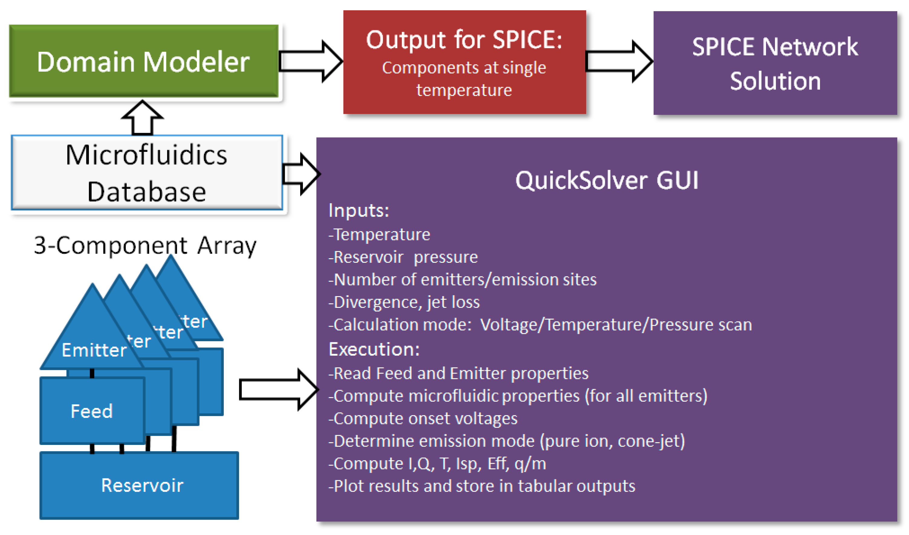
The domain modeler is a web-based modeling utility for the design of microfluidic components for eventual placement in an electrospray system network. The user designs a specific domain for which microfluidic properties of the domain are computed and displayed. The properties are computed with direct access to the properties database. There are two types of domains: feed system domains and emitter domains. Feed system domains include various flow media including cylindrical (capillary) or rectangular open channels, or porous media of similar shapes. Emitter domains incorporate the liquid Taylor cone charge emission physics, and the effects of the substrate on the Taylor cone base.

3.2.1. Feed System Models

The flow properties in feed system domains are computed with analytical viscous flow models or reduced order numerical solutions assuming laminar flow and channel dimensions below the capillary limit for which gravity can be neglected. Figure 4 shows a screenshot of the setup of a viscous flow feed domain consisting of a tapered porous conduit. On the left, the user selects options for the domain type, substrate, propellant, and temperature range. The entries for the domain shape and porosity properties are entered to the right of the domain shape design that defines the input variables. Once a property (field) is selected, a plot of the temperature dependence of this property is obtained by clicking “Run”. The chart shows the temperature dependence of the hydraulic resistance (in units of Pa·s/µL) of the porous medium in the defined flow direction. In order to export the component to a SPICE component library, the user clicks “Save”, and the component is saved with microfluidic properties at the temperature Tmin. Not shown in Figure 4 is the metadata text box providing information on how the various properties are computed. For viscous flow domains, the user can select in the “Field” box additional properties, including Laplace pressure, Reynolds number, wicking time, flow rate, and mass flow induced by the Laplace pressure as the conduit becomes fully wicked.

3.2.2. Emitter Domains

In order to set up an emitter component, the user selects an emitter type consisting of a Taylor cone substrate base design. Table 4 lists the currently supported emitter types and associated references used to develop the utility and component models. ESPET utilities compute emitter properties for a specified volume flow rate at the onset voltage assuming a cone-jet mode of operation. The default flow rate is given by the minimum flow rate, Qmin, at which a Taylor cone-jet can be sustained [12]:
Q min = 1 4 γ ε ε 0 ρ K ,
where γ is the liquid surface tension, ε is the relative permittivity, ε0 is the vacuum permittivity, and K is the liquid conductivity.
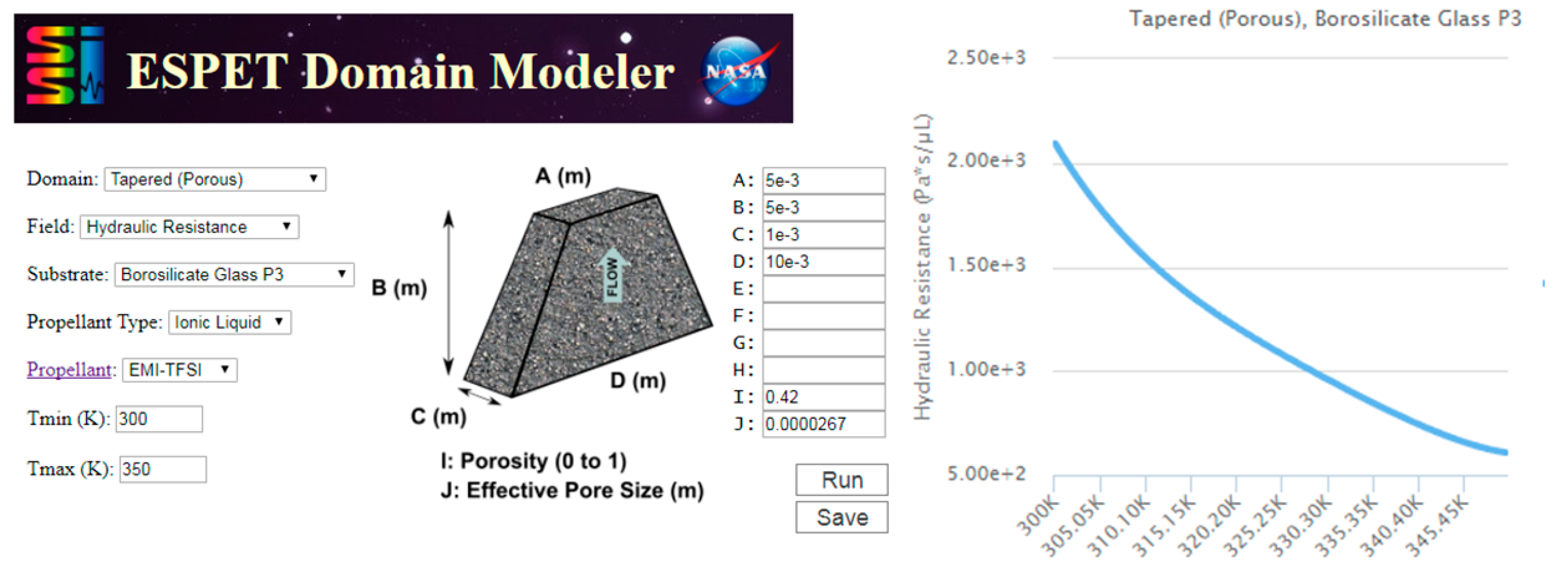
A number of outputs is produced by the emitter utility: onset voltage, hydraulic resistance of the emitter, the minimum flow rate, the droplet and ion currents, the charge to mass ratio of the spray current, thrust, 
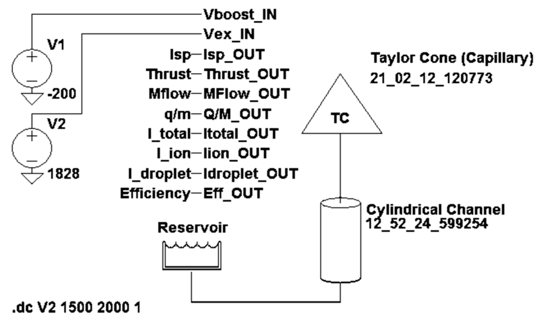
Isp, the maximum surface electric field, the mass flow, and the polydispersive efficiency. A screenshot of the capillary Taylor cone emitter domain modeler is shown in Figure 5. It illustrates the required user inputs for estimating individual emitter performance and for developing a SPICE component. Note that for this model involving an IL propellant, the user needs to define the polarity of the emitter (parameter F in Figure 5).
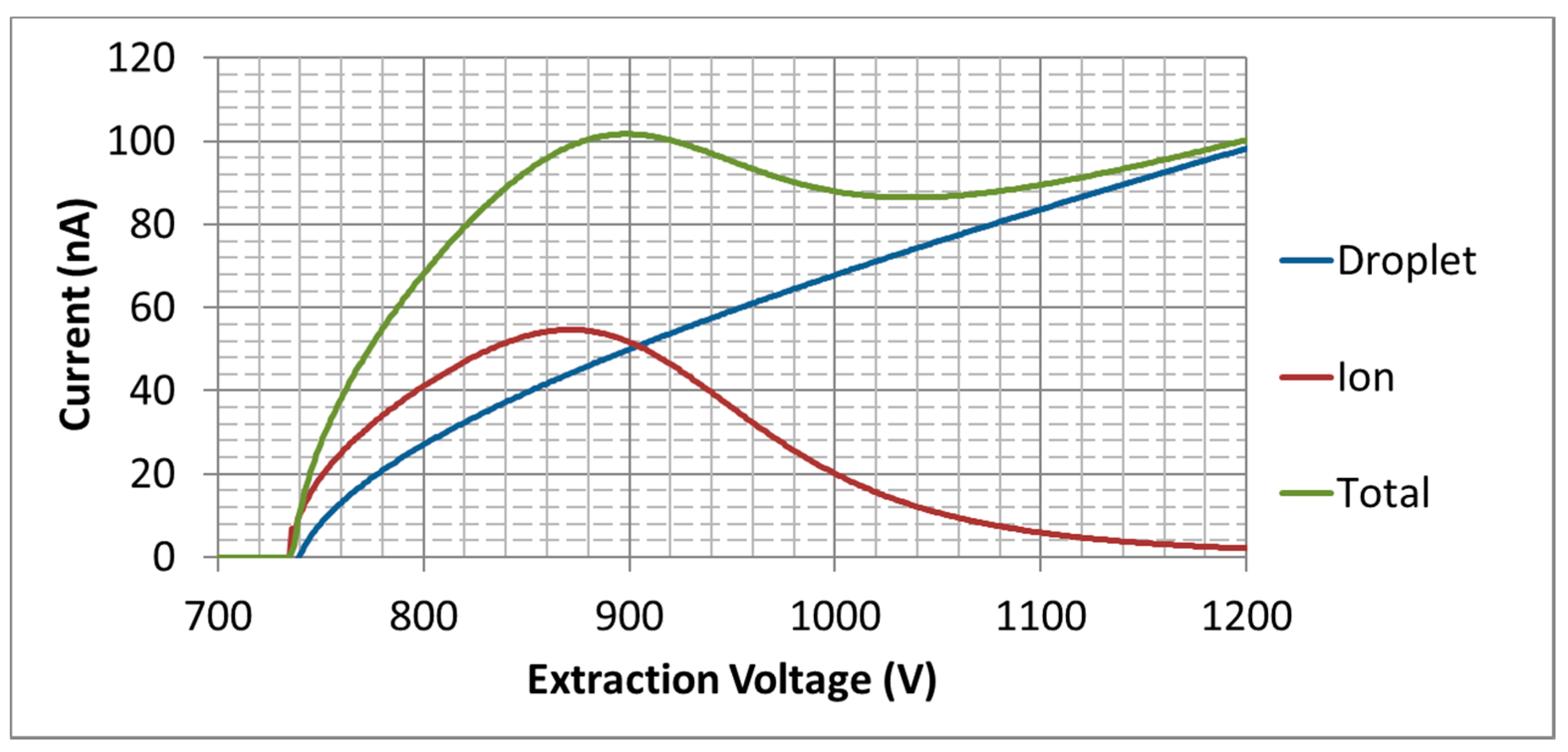
For dielectric propellants (e.g., ILs) the droplet current, Idroplet, is computed from the empirical expression derived by Gañán-Calvo et al. [47]:
I d r o p l e t = 2.6 I 0 ( Q / Q 0 ) 1 / 2 Q 0 = γ ε 0 ρ K , I 0 = ε 0 γ 2 ρ
The maximum cone-jet surface field is obtained from [11]:
E max = γ 1 / 2 K 1 / 6 ε 0 2 / 3 Q 1 / 6
We then follow the ion field evaporation theory of Higuera [39] and Coffman [17] to compute the ion field evaporation current from:
I i o n ( E max ) = A ( E max ) σ ( E max ) k B T h exp [ Δ G G ( E max ) k B T ]
where σ (Emax) is the surface charge density at the region of maximum field, k B and h are the Boltzmann and Planck constants, T is the temperature, ΔG is the ion solvation free energy, and G is the free energy associated with the external field. The effective field evaporation area, A(Emax), is estimated from:
A ( E max ) = π r e 2 , r e = 4 γ ε 0 E max 2
Equation (5) assumes field evaporation occurs at the neck of the cone-jet. Coffman provides justification to neglect the convection current in the field evaporation region near the Taylor cone tip. In this case the field evaporation current is equal to the conduction current given by:
I i o n ( E max ) = A ( E max ) K E max l
and the internal electric field, E max l , can be computed assuming a steady-state surface charge density from:
E max l = E max ε ( 1 + h K ε 0 ε k B T exp [ 1 k B T { Δ G G ( E max ) } ] )
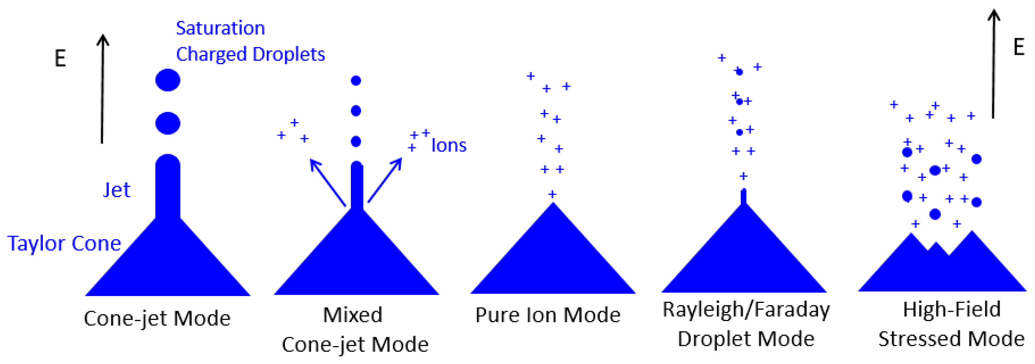
This approach neglects ion emission at the jet tip. Measurements by Gamero-Castaño [48] observed a substantial ion current fraction at high flow rates of a EMI-TFSI system, and concluded that ion emission occurs primarily at the jet tip at these conditions. At high flow rates, Emax is too low for measurable field evaporation. Currently, the ESPET cone-jet model does not include jet tip ion emission (high flow rate mixed ion-droplet regime).
Component models require that the microfluidic network provides input flow and pressure as a function of extraction field strength. This is straightforward for actively pressurized systems where the flow rate is given by the ratio between the pressure drop across the feed system and the feed system hydraulic resistance. For passively pressurized emitters, the electric field drives the flow. In a cone-jet mode, we compute the field-induced pressure to produce flow as an excess pressure beyond the onset voltage, V 0 , as proposed by Perez-Martinez [31]:
Δ p p s c a l e 2 ε 0 ( V e x 2 V 0 2 ) a 2 atanh 2 ( η 0 ) ( 1 η 0 2 ) 2 , a = 2 D / η 0 ,   η 0 = ( 1 + r c / D ) 1 / 2 .
where V e x is the extraction voltage, rc is the tip curvature for an externally wetted or porous emitter, or the capillary inner radius for an internally wetted or capillary emitter, and D is the tip to extractor distance. pscale is an empirical adjustable parameter that determines the fraction of the electric field-induced force that results in induced flow.
For emitters in a pure ionic regime (PIR), we follow the work of Coffman et al. [18]. This is still an area of active research and there are no simple analytical formulae that predict that a Taylor cone operates in a PIR. For both dielectric and LM propellants, it is known that pure ion emission is more probable for feed systems with high hydraulic resistance [13,16,18]. Coffman and coworkers [18] determined that the ion evaporation current for dielectric propellants with significant conductivities is inversely proportional to a dimensionless feed system hydraulic resistance parameter, CR:
I i o n = I min + B C R ( V e x V 0 ) C R = K E c r b a s e 2 p c ρ ( q / m ) R h y d ,   E c = 2 p c / ε 0 ,   p c = 2 γ / r b a s e
where rbase is the Taylor cone base radius and B is a slope parameter that Coffman et al. suggest is universal in that it applies to all dielectric propellants that operate in a conduction limited regime (liquid metals are known to operate in a space charge limited regime [
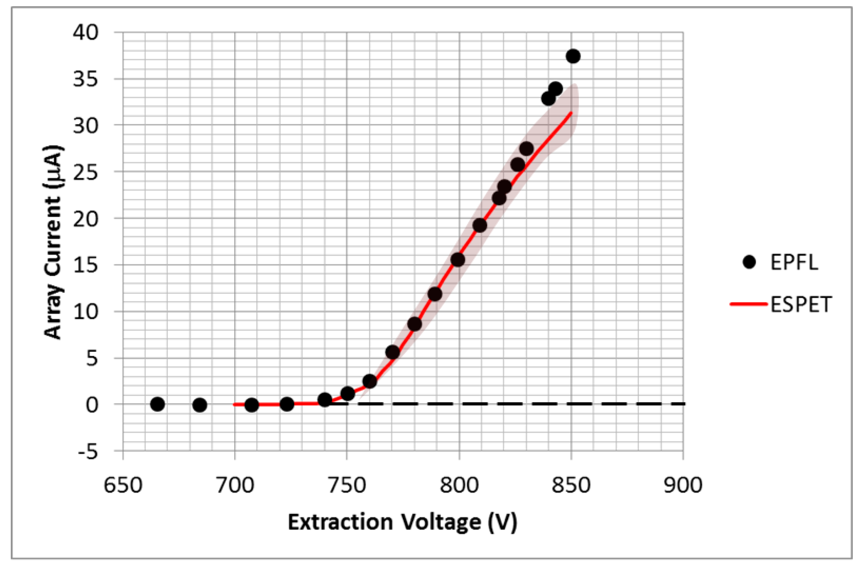
10]). The group of Lozano recently conducted single emitter measurements in the PIR. The measurements include a newly tested substrate consisting of a xerogel with very narrow pore-size distribution [31,43]. We also include measurements by Guerra-Garcia et al. [49] using borosilicate tips. Figure 6 plots the experimental voltage–current (VI) slopes against 1/CR to determine the value B. The data are in polarity pairs and show that only the EMI-BF4 results can be reasonably subjected to a linear regression. The derived slope for EMI-BF4 measurements corresponds to a value of B = 6.06 × 10⁻⁹ Ω−1. The time-of-flight measurements conducted by Perez-Martinez [31] demonstrate that the EMI-TFSI system operated in a cone-jet mixed ion-droplet regime and the relations in Equation (10) for P are thus not applicable.
The results in Figure 6 raise the question whether the B slope value is indeed universal. The data suggest that EMI-BF4 can operate in a PIR at lower values of CR than EMI-TFSI. Currently we propose that the user sets a propellant-dependent threshold value of CR at which the emitter starts to operate in a PIR. Our data survey suggests CR ≈ 3 for EMI-BF4, and at least 10 for EMI-TFSI. We also note that the numerical calculations by Coffman et al. [18] focused on systems with CR ≥ 1000, which is a regime normally applicable to externally wetted systems. Finally, using CR as the switching parameter neglects the role of the surface electric field, Emax, and does not do justice to the pioneering work of Coffman in navigating the extensive CR, Emax, and rbase stability phase space [17,18]. Critical in the future development of ESPET is finding an algorithm that incorporates these results properly. Nevertheless, a switching value of CR provides a means to turn on and off the PIR when analyzing array data, as demonstrated below.
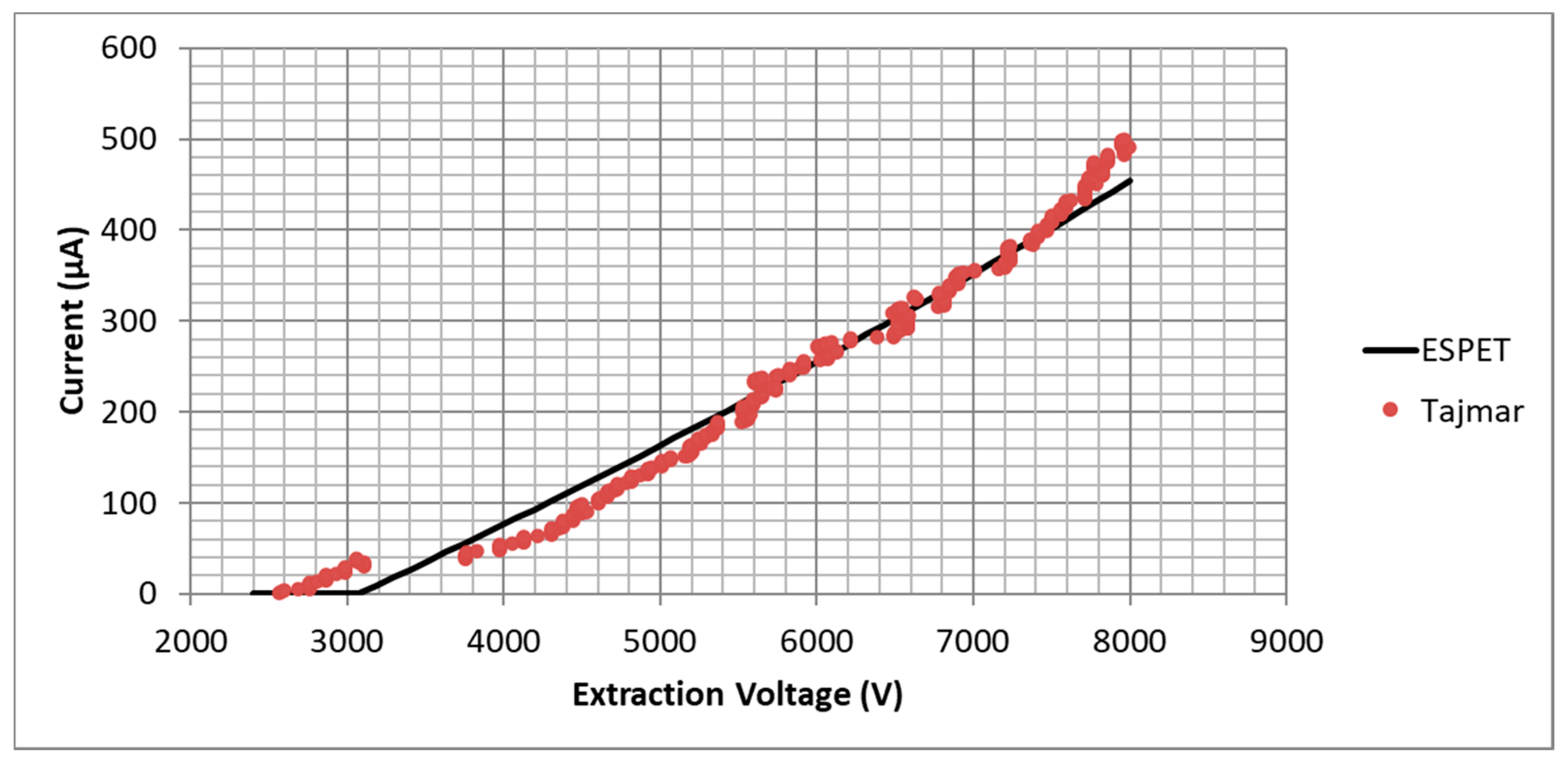
For LM systems, ESPET incorporates the theory introduced by Mair who derived a current–voltage expression for “low-impedance” liquid metal capillaries or low-impedance, grooved externally wetted emitters or emitters with roughened surfaces [13]:
I = 3 π 2 e M r b a s e γ cos α T 2 V o 1 / 2 ( ( V e x V 0 ) 2 1 ) ,
where M is the atomic mass of the liquid metal propellant, e is the unit charge, and αT is the Taylor cone half angle of 49.3°. For high-impedance LM Taylor cones (smooth externally wetted tips, or small capillaries), a flow-impedance (hydraulic resistance) factor is introduced:
I e m i t t e r = 3 π 2 e M r b a s e γ cos α T 2 V o 1 / 2 ( ( V e x V 0 ) 2 1 ) × [ 1 + 3 π r b a s e 2 R h y d 4 ρ V o 1 / 2 ( e / 2 M ) 1 / 2 ] 1 3 π 2 e M r b a s e γ cos α T V o 1 / 2 ( ( V e x V 0 ) 1 ) × [ 1 + 3 π r b a s e 2 R h y d 4 ρ V o 1 / 2 ( e / 2 M ) 1 / 2 ] 1 1 / Z 3 π 2 e M r b a s e γ cos α T V o 3 / 2 [ 1 + 3 π r b a s e 2 R h y d 4 ρ V o 1 / 2 ( e / 2 M ) 1 / 2 ] 1
where 
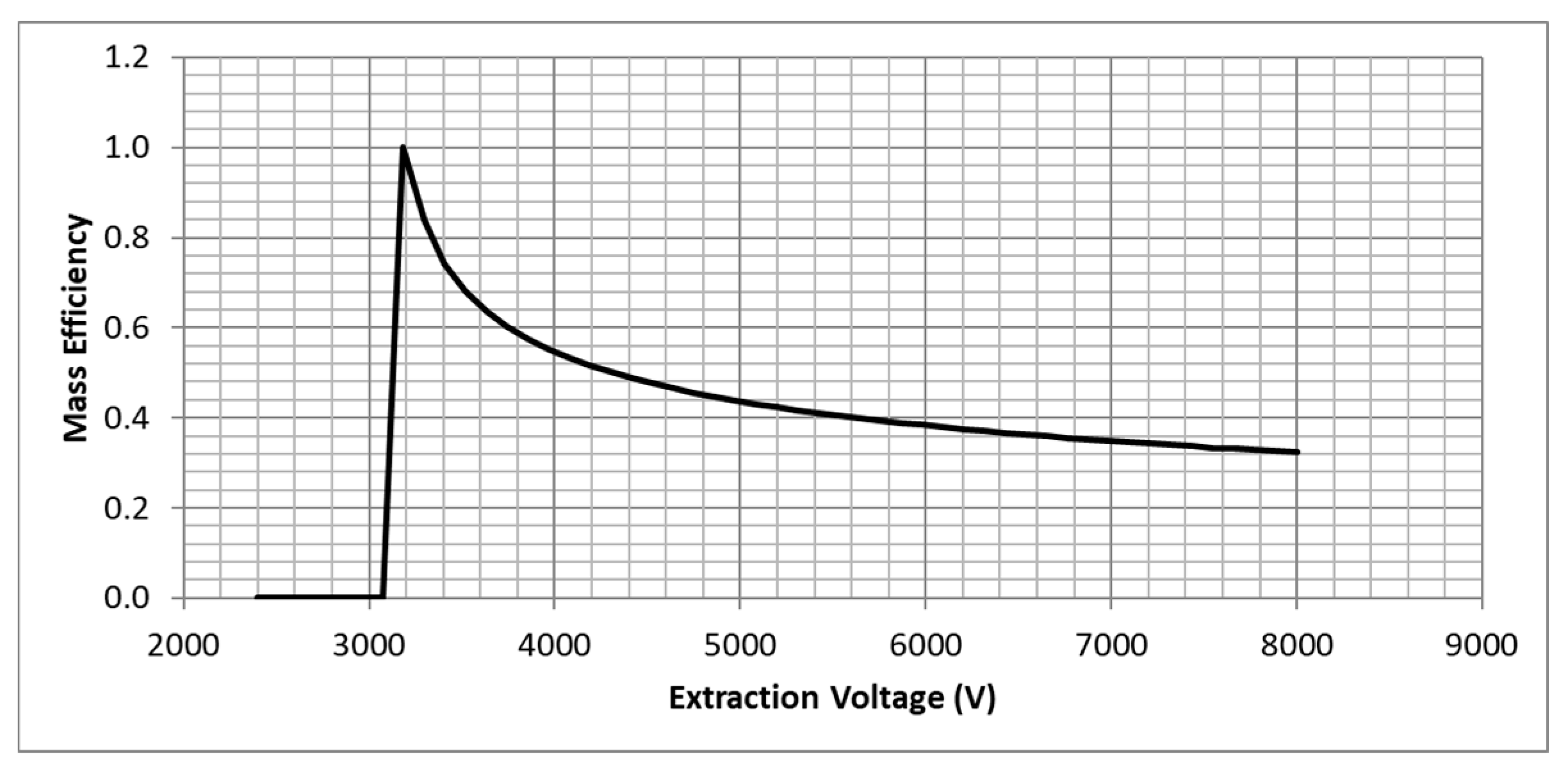
Z is the electric impedance. For LMs we also estimate the mass efficiency based on an empirical expression developed by Tajmar and coworkers for liquid indium systems [14]. The mass efficiency corresponds to the mass fraction of the output mass flow attributable to atomic ions, the remainder of the mass flow being due to droplets. The theory for droplet formation in LM systems is still underdeveloped.
Porous conical or edge emitters, and externally wetted emitters have the additional complication of multiple emission sites per emitter. Edge emitters can have hundreds of emission sites per centimeter. For typical IL contact angles, emission sites of porous substrate emitters are located at specific surface pores in areas of high surface curvature. Emission sites on externally wetted needle emitters are associated with surface protrusions that exceed the average roughness. The protrusions and pores form a base for a Taylor cone if sufficiently wetted by the propellant. Since the resulting Taylor cone bases and tip curvatures are subject to length scale distributions, each emission site is associated with a different onset voltage. In addition, the more displaced the pore is from the emitter tip or edge, the weaker the surface electric field, thus further broadening the distribution of onset voltages. As the voltage is raised, the number of emission sites exposed to field strengths exceeding the onset field increases. Unlike the single emission site VI curves, which are close to linear, those of multiple emission site emitters have a parabolic appearance [2,16].
Further complications arise when the Taylor cone base radii are greater than the pore size for highly wetted propellant/substrate combinations (small contact angles). A model for porous emitters must, therefore, also account for propellant pooling. In Section 5, we discuss benchmarking a porous model with multiple emission sites using experimental data that spatially resolves emission currents from different emission sites of a porous conical emitter and an externally wetted emitter.

3.3. Network Solver

3.3.1. SPICE Network Solver

The network solver uses the freely available SPICE electric circuit solver software. SPICE has the advantage of using a mature user interface with a range of simulation and output options. The graphical user interface (GUI) facilitates setting up a microfluidic network consisting of components, such as microfluidic transport channels, pressurized reservoirs, and Taylor cone emitters. Using the Hagen–Poiseuille/Ohm’s law analogy, the liquid conduits are representative of resistors and pressurized reservoirs are the equivalent of a voltage source. The user can also add a hydraulic capacitance or compliance through the use of a capacitor, which is useful for simulating time-dependent behavior. Currently, we do not have a domain model for producing a compliance component. The user must compute its value and enter the value in the capacitance component of a SPICE circuit. As mentioned in the previous section, Taylor cone emitters require specialized components since they operate both in an electrical and a microfluidic domain. For both hydraulic resistances and Taylor cones, the domain modeler computes its properties associated with a chosen propellant, substrate, and temperature. These properties are then saved into a SPICE component file that is transferred to a library of components that SPICE identifies when the user enters a new component to the system schematic.
The smart components, in addition to providing output flow and current, also provide outputs such as emitter thrust, specific impulse, and polydispersive efficiency. These outputs can be produced for a single extraction voltage output, or for an extraction voltage scan, such as the production of a voltage–current (VI) curve, which is graphically displayed. The user can also exploit special features of the SPICE simulator such as circuit optimization and the calculation of uncertainty bounds based on tolerances of properties provided by the user. The user has to separately download SPICE, for example, the LTspice version from Linear Technologies [50].

3.3.2. QuickSolver

Key drawbacks associated with the SPICE network solver are the time required for setting up a large array, complications associated with direct current (DC) voltage scans for porous systems with stochastic distributions of pore sizes, and the requirement to generate new components for every operating temperature of interest. The advantages of using SPICE are that there are no limits to the complexity of a microfluidic network, and that many features of SPICE can be used such as the graphing interface, the ability to apply tolerances and to conduct Monte Carlo, and worst-case scenario analysis of performance.
At the current state of electrospray propulsion technology, most designs can be described by a three-component, reservoir-feed-emitter microfluidic system, where solving for the volume flow rate is straightforward. For this reason, we have integrated the “QuickSolver” in the overall ESPET architecture (see Figure 3). The QuickSolver is accessed from the existing web user interface and is run from a separate GUI fully independent from the domain modeler.
The QuickSolver has several advantages. Component specification changes can be rapidly implemented within the QuickSolver GUI without the need to import a new component into the network. By accessing the database polynomials for the temperature dependence of propellant properties, it can instantaneously compute new performance parameters after changing the temperature. The QuickSolver can also handle the effects of design tolerances. Its organization is similar to that of the other ESPET pages. The code is written and organized in a way that new emitter models can easily be introduced. By using Python and a four-dimensional baseline matrix logic, we take advantage of extensive libraries such as routines for array data sorting. This is particularly important when treating multi-emission site emitters where the hydraulic resistance changes with the onset of new emission sites. In this case, the emission sites need to be sorted according to their onset voltages to allow for computing the hydraulic resistance of each emission site according to the number of active sites at a particular voltage.

4. Application of ESPET to Examples in the Literature

In this section, we apply ESPET models to several experimental examples from the literature, where we demonstrate its utility in interpreting prototype thruster performance data and in benchmarking unknown scaling parameters.

4.1. Actively Pressurized Capillary Emitters Using SPICE Option

We demonstrate the functionality of ESPET by making performance predictions for a simple single-emitter system and a small array of actively pressurized capillaries. We start with the simplest electrospray thruster design, an actively pressurized capillary emitter operated at room temperature. We compare this to the data published by Gamero-Castaño and Hruby [51] for a thruster resembling the colloid thruster used on the ST-7 Lisa Pathfinder mission [52]. The LTspice schematic of a single emitter system is shown in Figure 7. It consists of a pressurized reservoir, a capillary feed system, and a Taylor cone emission site at the end of the capillary emitter. The actively pressurized thruster operates at a single extraction voltage at which Taylor cone stability and emission are optimized. Thrust is adjusted with the acceleration or boost voltage and the mass flow is controlled by the pressure applied to the propellant reservoir. The Taylor cone is modeled in an on-off mode, where the spray properties are constant for extraction voltages above the onset voltage computed for the capillary/extractor geometry defined in the domain modeler. The voltages are applied to the inputs using LTspice voltage source components. We apply a −200 V boost voltage which represents the estimated energy lost by droplets in the jet. If there is an acceleration stage in addition to the extraction voltage, V e x , that voltage, V b o o s t , can be added to the assumed droplet energy loss. The total acceleration is given by V e x + V b o o s t . The thruster is operated in a positive current mode.
The feed system consists of custom components for a reservoir and a capillary. These components are generated by the domain modeler that is linked to the microfluidics database. Alternatively, the reservoir can be replaced by a voltage source, which is the equivalent of a pressure source in the microfluidic realm. For both options, the user enters pressure in units of Pascal. Flow and hydraulic resistance units are µL/s and Pa·s/µL, respectively.
Table 5 shows the output results for two input pressures that produce mass flows equivalent to those used when testing the Busek capillary colloid thruster with a EMI-TFSI propellant [51]. The pressure was adjusted to match the quoted mass flow because the authors did not accurately specify the length of their capillary feed system which controlled the hydraulic resistance of the overall system. The only substantial discrepancy between the experimental results and ESPET is seen in the derived thruster efficiency, where the ESPET inefficiency is only based on the assumed 200 V loss of extraction voltage due to Ohmic losses in the jet. The polydispersive efficiency, attributable to the distribution of q/m values in the accelerated spray, is close to 1 since at the respective high flow rates, ion evaporation is predicted to be very low. Additional inefficiency is introduced through beam divergence. The higher experimental inefficiency is consistent with the lower thrust and Isp observed in the experiments. Overall, however, the agreement is very satisfactory.
To test the model in a low flow rate regime that approaches the minimum flow rate, we instructed SPICE to scan a range of low reservoir pressures corresponding to a volume flow rate scan near the minimum flow rate. Figure 8 shows the total, ion, and droplet currents versus the volume flow rate generated in a pressure scan (voltage scan in SPICE) at volume flow rates near the minimum flow rate, identified by the vertical dashed line. The ion field evaporation current is observed to increase below flow rates of 6 × 10⁻⁶ µL/s. Slightly above the minimum flow rate, the ion and total currents reach a maximum. This contradicts what is found experimentally [11,51], where the ion field evaporation current continues to increase with decreasing flow rate. We believe that in this regime of high surface electric fields, some of the assumptions underlying Equations (4)–(8) are no longer valid. The model, however, identifies the transition region from a nearly pure droplet regime to one where there is significant ion field evaporation.
Figure 9 shows for the same system similar plots for thrust, Isp, q/m, and polydispersive efficiency. For the latter, we assume that the ion current is composed of equal fractions of monomer (single positive ion) and dimer (positive ion complexed with an ion pair) ions. As expected, the thrust increases with flow rate, while the Isp decreases. Thrust and Isp are related to the average q/m of the spray, which declines with flow rate. At the highest flow rate of the chart, the polydispersive efficiency is close to 1 because ESPET predicts that the spray is almost entirely due to droplets. The efficiency decreases as the spray becomes increasingly a mixture between droplets and ions with decreasing flow rate. At the lowest flow rate, the efficiency is about 50% due to the still significant presence of charged droplets in the spray (see Figure 8).
Figure 10 shows a SPICE schematic of an array of three emitters using the components of the thruster in Figure 5. In Figure 11 we show the total thrust and Isp of the system as a function of the acceleration voltage. The latter is scanned from 0 to 500 V, while keeping the extraction voltage constant at 1828 V. The system is operated at a 4.1 kPa reservoir pressure (see Table 5). We still assume a −200 V potential drop in the jet.
When assigning tolerances to component parameters, the actual parameter value is set through a random number generator by LTspice reflecting the 1σ tolerance. For example, the hydraulic resistances of the feed capillaries in the network of Figure 10 can be affixed a 10% tolerance. The user can then choose several Monte Carlo “trajectories” to compute the distribution of possible performance outcomes. Thus, ESPET in conjunction with the LTspice Monte Carlo feature is well suited for predictions of the emission uniformity of new electrospray array designs. In addition to a Monte Carlo analysis, LTspice also offers “worst-case” analysis, where the network performance is computed at the extremes of component values specified with a tolerance. This provides for a more direct way of extracting quantitative information on the range of outputs of emitter components.

4.2. Passively Driven Capillary Emitter Array

In this section, we apply both SPICE and QuickSolver solutions to the analysis of results obtained for a passively driven micro-machined capillary emitter array operated on an EMI-BF4 IL propellant, as reported by Dandavino et al. [1] of the Ecole Polytechnique Federale de Lausanne (EPFL). The array has a total of 127 emitters. The thruster was operated passively (i.e., the reservoir pressure was zero), and the flow was induced by the electric field. First, we compare the average emitter performance reported by Dandavino et al. to the outputs of a SPICE circuit for a single emitter shown in Figure 12.
Two feed components are shown in Figure 12. The overall feed hydraulic resistance is dominated by the much narrower emitter inner diameter. The inner diameter of the emitter is quoted to be 7.9 ± 0.5 µm. We adjusted the emitter extractor gap to match the onset voltage, and then adjusted a scaling factor, pscale, in Equation (9) to match the quoted mass flow. This resulted in pscale = 0.0085.
The results averaged over the array for a single thruster are tabulated in Table 6 for an extraction voltage of 850 V, which is ~90 V above onset. The comparison to data reported by Dandavino et al. (EPFL) clearly shows that ESPET underestimates the current and q/m, while overestimating the efficiency, thrust, and Isp. Figure 13 shows the modeled VI behavior for droplets and ions based on the cone-jet model incorporated in the passive capillary emitter component. The dashed line identifies the voltage at which Dandavino et al. report their average emitter performance data. As is seen, this falls in the regime below the current maximum, where the ion current fraction, fion, is high, and where the assumptions of the cone-jet model are less valid. Furthermore, there is the possibility that some thrusters are operating in the PIR. For the present analysis, we make the assumption that the source of the discrepancy between the modeled and measured emitter performance is that some emitters operated in a cone-jet mode while others operated in the PIR.
We further postulate that such a non-uniformity of emission across the array is primarily caused by the tolerances associated with the capillary inner diameter which determines the feed resistance and onset voltage. The hydraulic resistance is proportional to the inverse fourth power of the inner diameter. Consequently, a ~6% tolerance should have a marked effect on the distribution of hydraulic resistances, and thus the flow through the Taylor cones.
Modeling of the full 127 emitter array would be a large undertaking using the SPICE network solver. We, therefore, used the QuickSolver to model the non-uniformity introduced by the emitter diameter tolerance in this borderline cone-jet case. We also introduced mode-switching based on the CR parameter (Equation (10)). Table 7 compares the emitter-averaged values at an extraction voltage of 850 V to the data listed by Dandavino and coworkers (EPFL) after optimization of several benchmarking inputs listed in Table 8. Figure 14 shows the comparison to the experimental VI curve (EPFL) of the array (total current). The red curve was computed for 127 emitters and is close to an average computed for a substantially larger number of emitters (>1000). The shaded area reflects the QuickSolver solution space for several 127 emitter runs.
The statistics associated with the shading in Figure 14 is entirely attributable to the variance of the emitter capillary radius given by the tolerance quoted by Dandavino et al. [1] (Table 8). The critical benchmarking parameters are the CR mode switching limit, pscale, and B, the pure ionic model voltage–current slope parameter. These parameters were adjusted to optimize the comparison in Table 7. The optimized pure ionic mode slope parameter B is set to 1.8 × 10⁻⁸ Ω−1, which is a factor of 3 greater than that derived from the data in Figure 6. pscale is higher than what we found using the SPICE model. The QuickSolver model predicts that 46% of emitters are in pure ionic mode. The remaining emitters are in mixed cone-jet mode.
ESPET correctly renders the curvature of the onset in Figure 14, a direct consequence of the variance in onset voltages introduced by the tolerance of the emitter radius (and thus the Taylor cone base radius). The experiments by Dandavino et al. [1] included several VI curves for different acceleration (boost) voltages. We plot only the curve for zero boost voltage. The full input deck for the calculations producing the results in Figure 14 can be obtained via the ESPET website (espet.spectral.com) from the capillary IL QuickSolver example.

4.3. Externally Wetted Liquid Metal Emitter

In our final example comparing against data from the literature, we use ESPET to model an externally wetted LM emitter. The ESPET model for such emitters is tested against the data reported by Tajmar [14] on an indium wetted tungsten needle (see Figure 2 in [14] for a microscopic image of the needle tip). Figure 15 compares the experimental VI data to ESPET QuickSolver model outputs. Table 9 lists the parameters used for the simulation, several of which were taken directly from Tajmar [14].
The only parameter with high uncertainty, and for which no measurement was provided, is the film thickness, δ, which controls the hydraulic resistance of the emitter. For the hydraulic resistance, ESPET uses the expressions reported by Mair [13] for a cylindrical (e.g., wire) conduit:
R h y d = 3 μ L 2 π r δ 3 ,
where μ is the liquid dynamic viscosity, L is the conduit length, and r is the conduit radius. For a cone with a half angle, α, curvature, r c , and height, H, the hydraulic resistance is given by:
R h y d = 3 μ ln ( 1 + H tan α / r c ) 2 π δ 3 tan α
We found that the VI results were insensitive to the film thickness for values above 0.3 μm. Below this value, the VI slope drops with declining film thickness and the agreement with experiment becomes poorer. This suggests that the needle was operated in a low Z regime where the feed hydraulic resistance is immaterial in the VI relationship (expression in square brackets of Equation (12) is close to 1). For this needle, Tajmar reports a mass efficiency of 52.5% at a current of 100 μA, which is in good agreement with the ESPET prediction of 50%. The ESPET mass efficiency versus voltage curve is shown in Figure 16. The good agreement with experiment is further evidence of this needle operating in a low Z regime because the empirical mass efficiency model was benchmarked for low Z systems [14].

5. The Development of Models for Emitters with Multiple Emission Sites

We are not aware of any models that describe the formation of multiple emission sites from externally wetted and porous emitters. In this section, we introduce the ESPET-assisted development of empirical models for such emitters. The models are benchmarked against experiments that were conducted in the vacuum facility at Busek Co.

5.1. Externally Wetted Emitter Using Ionic Liquid

We applied ESPET to the analysis of electrospray experiments using a tungsten needle emitter wetted with an EMI-TFSI propellant. Figure 17 shows a scanning electron microscope (SEM) image of the emitter tip which is found to have a 6 μm radius of curvature and a half angle of 15°. The 2 mm long needle was etched to have a roughened surface to improve propellant wetting. Figure 17 also shows the current probe geometry used to measure spatially resolved emission currents. The purpose of the setup was to spatially resolve individual beamlets in order to identify currents from separate emission sites, each associated with its own Taylor cone, and to observe the transition from stable cone-jet operation to a stressed multi-jet regime [19]. The emitter and extractor with a 1.5 mm diameter orifice were placed on an X-Y translation stage. The current probe consisted of a coaxial cable with a copper inner electrode with a 71 µm inner diameter that is surrounded by a Teflon insulator and a copper outer electrode with an 864 µm out diameter. The inner electrode is used to monitor the current as the probe moves across the X-Y plane. The outer electrode is grounded to prevent charging of the insulator. The probe was situated 0.5 mm behind the extractor which had an approximate 0.2 mm distance to the emitter tip.
Examples of spatially resolved current measurements in positive polarity operation are shown in Figure 18 for extraction voltages of 1400 and 1500 V. The figure shows the outlines of the extraction aperture. At the lower voltage, two beamlets are identified. They are numbered in sequence of appearance. Beamlet 1 appeared at ~1000 V, and beamlet 2 at 1200 V. Beamlet 1 is considerably off center, which we associate with a Taylor cone location that is away from the tip (off axis), where the radial component of the electric field is significant, leading to emission at large axial angles. At 1500 V, we observe three additional beamlets labeled 3, 4a, and 4b. Beamlet 3 appears at a lower voltage than beamlets 4a and 4b, which appear simultaneously. Beamlet 1 now appears as if it has split into multiple components, which we associate with instability, possibly a stressed multi-jet mode. At higher voltages, more beamlets exhibit a similar diffuse appearance, accompanied by higher angular emission. Examination of the stability of individual beamlet currents also indicates less stable emission from sites with a diffuse appearance. The spatial current maps look very similar in the negative polarity mode below 1500 V.
The ESPET model for externally wetted emitters assumes that emission sites are formed at inhomogeneities of the surface that can be characterized by a mean surface roughness, Ra, with an associated standard deviation. The surface roughness creates the protrusion of emission sites and defines their respective curvature. In addition, the propellant conduit to the tip is modeled as semi-cylindrical or rectangular grooves with a specified radius or width. Table 10 lists the ESPET input parameters chosen for the experimental emitters. The roughness is chosen from a visual estimate of the tip SEM image (Figure 17). Similarly, the groove diameter is chosen from a groove seen in the image. We assume four such grooves leading to the emission tip. The number of emission sites can be estimated from the ratio of the total tip surface area ( 2 π r t i p 2 ) to the average cross section of an emission site protrusion ( π r s i t e 2 ). With rtip = 6 μm and rsite = 2.8 μm, we get slightly more than nine emission sites, which we have rounded to 10. The model then determines the 10 rsite values using random number generation, and at each voltage determines which of the wetted protrusions have surface fields exceeding the onset voltage.
Since the experiment involved only a single emitter, and because our estimate for the roughness standard deviation (Table 10) is relatively high, we computed performance averages for 1000 emitters to compare to the experimental data. Even for that number of emitters, the variance in the outputs from run to run was significant, nicely reflecting the sensitivity to the roughness parameters. We, therefore, must assume that a model without detailed surface property information on the experimental tip will have substantial uncertainties when comparing to a single tip. Figure 19 compares the positive polarity data to four ESPET runs consisting of 1000 emitter averages. Given the uncertainties in characterizing the experimental emitter tip, the agreement between the experimental data and the model runs are very satisfactory. The experimental data is nicely bracketed by the model runs at higher voltages. Between 1200 and 1400 V, prior to the onset of unstable emission, the model overpredicts the current. As we see below, the model as implemented predicts a more rapid increase in the number of active emission sites than seen in the experiment. For the ESPET runs, non-dimensional hydraulic resistance values, CR, exceed 100, and the system is predicted to be in pure ionic mode for CR values exceeding 20 for EMI-TFSI. We do not have time-of-flight data that produce q/m distributions of the spray to verify this.
Figure 20 compares the observed number of emission sites for negative and positive polarity as a function of extraction voltage (absolute value) to the ESPET predictions which consist of a 1000 emitter average. Curiously, the negative polarity exhibits almost twice as many emission sites above 1500 V. Since the onset voltage only depends on surface morphology and surface tension, and, therefore should not depend on polarity, the larger number of observed beamlets may hint at higher instabilities in the negative mode possibly leading to multiple beamlets from a single site. The ESPET model predicts a faster rise in the number of emission sites with voltage. We attribute this to the model assumption that the external field is the same at all emission sites. The surface field, however, declines from the axial tip position to larger axial distances on the tip. We are working on introducing the emission site position and position-specific surface field into the model. We believe that this would bring the model in closer correspondence with the growth in emission sites seen in the experiment.
The experimental onset voltage is higher than what the model predicts. This can be reconciled with the fact that the first experimental emission site can be assumed to be significantly off axis on the tip, as evidenced by the high axial angle of the detected beamlet. At such a location, the electric field strength is weaker. We conclude that despite the uncertainties in tip roughness and propellant transport, the ESPET model incorporating multiple emission sites makes reasonable predictions.

5.2. Conical Porous Glass Emitter Using Ionic Liquid

In this section, we apply ESPET to the analysis of spatially resolved current measurements from a single porous borosilicate glass emitter manufactured at Busek. The emitter was operated with the EMI-TFSI ionic liquid propellant. Figure 21 is a microscopic image of the conical emitter. Table 11 specifies the salient properties of the emitter and feed system. The conical tip is connected to a base that acts as the feed system and has a larger pore size and a higher permeability. The same probe geometry shown in Figure 17 was used to characterize the emission of this porous emitter.
Unlike the externally wetted emitter examined in the previous section, the spatially resolved current maps do not reveal instabilities in the emission of specific emission sites. All resolved emission sites appear unique and maintain their angular direction as the extraction is ramped up. Figure 22 shows the growth in the number of emission sites versus extraction voltage for the two polarities. The first emission site turns on around 1100 V for both polarities. This is substantially lower than an onset voltage of V0 = ~2300 V expected from the information in Table 11, assuming that the Taylor cone base is comparable to the average pore size. The substantially lower onset voltage implies a significantly greater Taylor cone base radius than the average pore radius of ~0.65 μm. The observed onset voltage is consistent with a base radius of ~8 μm. This large radius could be explained by significant propellant pooling outside of the orifice of the supporting pore. Alternatively, the low onset voltage could be explained by larger, possibly shallow, pore openings at the surface that can support menisci with larger radii.
The distribution of pore sizes inferred from the quoted bulk pore size ranges cannot explain the broad range of observed onset voltages. Higher onset voltages can be attributed to smaller base radii and/or weaker fields associated with sites that are off the tip axis. Figure 22 indicates that the emitter can support at least 12 emission sites. The tip surface area (i.e., the area of high curvature) can accommodate less than four Taylor cones if they all had a base radius of 8 μm. Thus, as new sites turn on, their Taylor cone base radii must become smaller. In our efforts to benchmark against this experimental data, we integrated following the empirical function in ESPET for the Taylor cone base radius, bi, as a function of emission site number, i:
b i = b 0 [ 1 ( i 1 N max 1 ) 1 / 4 ] + r 0 ,
where r0 is the pore radius of the medium, b0 is the initial Taylor cone base radius, and Nmax is an adjustable parameter that corresponds to the maximum number of emission sites. For i = Nmax, bi equals r0, the bulk pore radius value. Figure 22 compares predicted emission site growth to the experimental data, showing reasonable agreement. There is stochastic variance to the model curves in Figure 22, but since only the pore size distribution is affected by a standard deviation, and the pooling base radius is significantly larger than the pore size, the variance is minor except for site number approaching Nmax.
In the previous case of externally wetted emitters with multiple emission sites, the hydraulic resistance was computed from assumed surface grooves that facilitate the transport of the propellant. We further assumed that each emission site was independent of the others in terms of its hydraulic resistance. For the present conical porous emitters, a model making this assumption failed to reproduce the observed behavior. This can be rationalized by the assumption that most of the conical volume of the tip can feed a single emission site, but as additional emission sites turn on, each site will be competing for the flow in the emitter. The total hydraulic resistance of the emitter does not change with an increasing number of emission sites, but the hydraulic resistance associated with the propellant feed of the individual Taylor cones will be proportional to the number of active sites:
1 R c o n e = i = 1 N 1 R i N R s i t e
R s i t e N R c o n e
where Rcone and Rsite are the hydraulic resistances of the full emitter cone and the individual emission sites, respectively, and N is the number of active sites. The steadily increasing hydraulic resistance for individual emission sites would explain why we do not observe instabilities at higher voltages. A higher effective hydraulic resistance has the effect of choking the flow with increasing electric field, thus stabilizing the emission. This is also manifested in the near constant current that we observe for individual emission sites after a rapid increase near onset.
Figure 23 compares the experimental VI curves for positive and negative polarity to ESPET outputs using the model described above. The ESPET parametric inputs are listed in Table 12. The model correctly reproduces the slightly lower current in the negative polarity. The modeled current exhibits small upward and downward steps at voltages where new emission sites become active. The upward steps can be attributed to new emission sites operating in cone-jet mode, while we attribute the downward steps to the onset of pure ionic mode emission sites. This is verified when examining the average charge-to-mass ratio or Isp, where sharp declines in Isp are observed when cone-jet emission sites add charged droplets to the spray. Time-of-flight (TOF) data recorded in the laboratory also confirm a high Isp that sporadically drops consistent with a system that operates close to the cone-jet–PIR transition region. The TOF data and detailed q/m analysis are being prepared in a separate, more exhaustive, report on the porous emitter experiments and model.
The benchmarked parameters in Table 12 show a maximum number of emission sites, Nmax, of 20, suggesting that the Taylor cones associated with the emission sites observed near the maximum experimental extraction voltage are still significantly larger than the nominal pore size. The CR limit value is the same applied to the analysis of the externally wetted needle case of the previous section. The slope parameter, B, however, is ~35% higher, showing some inconsistency in the models. The quality of the experimental data, however, is significantly greater for the porous glass emitter. The pressure-field scaling parameter, pscale, is the same value applied to benchmarking the capillary array (Section 4.2) using the EMI-BF4 propellant.

6. Conclusions

ESPET offers a framework for multiscale modeling of electrospray propulsion systems from propellant reservoir to charge emission for systems operating under stable Taylor cone conditions. It incorporates models for internally wetted, externally wetted, and porous emitters, and includes properties for several dielectric (ILs) and liquid metal propellants. ESPET incorporates a database of microfluidic properties of propellants, substrates, and their interfacial properties. Polynomials for the temperature dependence of critical propellant properties are provided, allowing rapid temperature optimization of systems. ESPET has an easy-to-use interface to the SPICE electric circuit solver software for microfluidic network design, solution, analysis, and outputs. For simple three-component systems, an internal solver, the QuickSolver, can be used for rapid analysis.
We report successful tests on simple IL electrospray systems involving individual capillary emitters and capillary arrays, and an LM example involving an externally wetted needle. For these cases, we compared the ESPET output to data reported in the literature. We then used ESPET to analyze recent experimental data on an IL-propelled externally wetted needle and a conical porous emitter, both of which exhibit multiple emission sites that were associated with separate beamlets resolved by a spatial current detection system. The analysis led to the development and benchmarking of multi-emission site models that produced satisfactory agreement with the observed voltage–current curves.
In its current state, ESPET can be regarded as a database of electrospray microfluidic properties and analytical models. As demonstrated, it can already be used as a research tool for the analysis and benchmarking of experimental results, and the evaluation of parameter sensitivities. We hope that with time and the incorporation of new properties and benchmarked models, ESPET will increasingly become predictive. Spectral Sciences Inc., freely shares the online tool to the electrospray propulsion community in the hope that this encourages users to share their experimental data and new models. Requests for an account can be made through the SSI website: http://www.spectral.com/contact-us-about-espet/.
There is much room for improvement. A robust model to identify conditions leading to pure ionic emission for arbitrary dielectric propellants is still necessary. Until such a model is available, empirical approaches will be necessary. Additional features to be developed for dielectric systems include an alternating, time-dependent polarity mode, which will require the addition of new components such as hydraulic capacitances (compliances), and predictions of electrochemical decay times. ESPET needs estimates of sources of inefficiency in addition to the polydispersive efficiency, such as energy inefficiency due to ohmic losses in the cone-jet transition region, divergence losses, ionization efficiency affected by decay of complex ions in the acceleration region (e.g., dimer, trimer ions), and extraction efficiency (losses on extractor electrode). Explicit calculation of the field strength as a function of the position on a tip of porous or externally wetted emitters would improve the multi-emission site model and could lead to a model for the divergence of such emitters as a function of extraction voltage. Poor extraction efficiency due to divergence can be a source mechanism for failure and limit how hard multi-emission site emitters can be driven in terms of the extraction field. Jorns and coworkers have embarked on an effort to extend ESPET to predicting thruster lifetimes using novel uncertainty quantification techniques [53]. Significant progress in lifetime assessment was made by Wirz and coworkers, who reported combined experimental and modeling studies for estimating the lifetime of capillary emitter systems based on an extraction and acceleration grid impingement mechanism [54,55,56].

Author Contributions

Conceptualization, B.S.P., R.A.D.; methodology, All; software, B.S.P.; validation, R.A.D.; formal analysis, All; investigation, All; resources, R.A.D.; writing—original draft preparation, R.A.D., Y.-h.C.; writing—review and editing, R.A.D.; project administration, R.A.D.; funding acquisition, R.A.D., B.S.P., Y.-h.C. All authors have read and agreed to the published version of the manuscript.

Funding

ESPET was developed under a NASA Small Business Innovative Research (SBIR) grant under contract no. NNX16CC23C, technical monitor: John T. Yim. The authors are also grateful for an IR&D grant from Spectral Sciences Inc.

Acknowledgments

The authors acknowledge Y. Wang and H. Song (CFD Research Corporation) for microfluidics contributions towards the development of ESPET and Paulo Lozano of the Massachusetts Institute of Technology for many helpful discussions and for sharing his research results.

Conflicts of Interest

The authors declare no conflict of interest.

References

  1. Dandavino, S.; Ataman, C.; Ryan, C.N.; Chakraborty, S.; Courtney, D.; Stark, J.P.W.; Shea, H. Microfabricated electrospray emitter arrays with integrated extractor and accelerator electrodes for the propulsion of small spacecraft. J. Micromechanics Microengineering 2014, 24, 075011. [Google Scholar] [CrossRef]
  2. Courtney, D.G.; Li, H.Q.; Lozano, P. Emission measurements from planar arrays of porous ionic liquid ion sources. J. Phys. D Appl. Phys. 2012, 45, 485203. [Google Scholar] [CrossRef]
  3. Legge, R.S.; Lozano, P.C. Electrospray propulsion based on emitters microfabricated in porous metals. J. Propuls. Power 2011, 27, 485–495. [Google Scholar] [CrossRef]
  4. Gassend, B.; Velasquez-Garcia, L.F.; Akinwande, A.I.; Martinez-Sanchez, M. A Microfabricated Planar Electrospray Array Ionic Liquid Ion Source With Integrated Extractor. Microelectromechanical Syst. J. 2009, 18, 679–694. [Google Scholar] [CrossRef]
  5. Velasquez-Garcia, L.F.; Akinwande, A.I.; Martinez-Sanchez, M. A Planar Array of Micro-Fabricated Electrospray Emitters for Thruster Applications. J. Microelectromechanical Syst. 2006, 15, 1272–1280. [Google Scholar] [CrossRef]
  6. Taylor, G.I. Disintegration of water drops in an electric field. Proc. R. Soc. A 1964, 280, 383–397. [Google Scholar]
  7. De la Mora, J.F. The effect of charge emission from electrified liquid cones. J. Fluid Mech. 1992, 243, 561–574. [Google Scholar] [CrossRef]
  8. De la Mora, J.F. The fluid dynamics of Taylor cones. Annu. Rev. Fluid Mech. 2007, 39, 217–243. [Google Scholar] [CrossRef]
  9. De la Mora, J.F.; Loscertales, I.G. The current emitted by highly conducting Taylor cones. J. Fluid Mech. 1994, 260, 155–184. [Google Scholar] [CrossRef]
  10. Gamero-Castaño, M.; Aguirre-de-Carcer, I.; De Juan, L.; de la Mora, J.F. On the current emitted by Taylor cone-jets of electrolytes in vacuo: Implications for liquid metal ion sources. J. Appl. Phys. 1998, 83, 2428–2434. [Google Scholar] [CrossRef]
  11. Gamero-Castaño, M.; de la Mora, J.F. Direct measurement of ion evaporation kinetics from electrified liquid surfaces. J. Chem. Phys. 2000, 113, 815–832. [Google Scholar] [CrossRef] [Green Version]
  12. Loscertales, I.; de la Mora, J.F. Experiments on the kinetics of field evaporation of small ions from droplets. J. Chem. Phys. 1995, 103, 5041–5060. [Google Scholar] [CrossRef]
  13. Mair, G. The effects of flow impedance on the current-voltage characteristics of liquid-metal ion sources. J. Phys. D Appl. Phys. 1997, 30, 1945. [Google Scholar] [CrossRef]
  14. Tajmar, M. Influence of Taylor cone size on droplet generation in an indium liquid metal ion source. Appl. Phys. A 2005, 81, 1447–1450. [Google Scholar] [CrossRef]
  15. Tajmar, M. Indium capillary liquid-metal-ion-source operation in the flow resistance regime. J. Phys. D Appl. Phys. 2004, 37, 3056. [Google Scholar] [CrossRef]
  16. Courtney, D.G.; Shea, H. Influences of porous reservoir Laplace pressure on emissions from passively fed ionic liquid electrospray sources. Appl. Phys. Lett. 2015, 107, 103504. [Google Scholar] [CrossRef] [Green Version]
  17. Coffman, C. Charge Emission from Electrified Ionic Liquid Menisci: Fundamental Phenomena and Applications to Micropropulsion. Ph.D. Thesis, Aeronautics and Astronautics Dept, Massachusetts Institute of Technology, Cambridge, MA, USA, 2016. [Google Scholar]
  18. Coffman, C.; Martínez-Sánchez, M.; Higuera, F.J.; Lozano, P.C. Structure of the menisci of leaky dielectric liquids during electrically-assisted evaporation of ions. Appl. Phys. Lett. 2016, 109, 231602. [Google Scholar] [CrossRef]
  19. Cloupeau, M.; Prunet-Foch, B. Electrohydrodynamic spraying functioning modes: A critical review. J. Aerosol Sci. 1994, 25, 1021–1036. [Google Scholar] [CrossRef]
  20. SPICE. Available online: http://embedded.eecs.berkeley.edu/pubs/downloads/spice/ (accessed on 30 June 2020).
  21. SQLite. Available online: https://www.sqlite.org/ (accessed on 30 June 2020).
  22. Fröba, A.P.; Kremer, H.; Leipertz, A. Density, refractive index, interfacial tension, and viscosity of ionic liquids [EMIM][EtSO4], [EMIM][NTf2], [EMIM][N(CN)2], and [OMA][NTf2] in dependence on temperature at atmospheric pressure. J. Phys. Chem. B 2008, 112, 12420–12430. [Google Scholar] [CrossRef]
  23. Zaitsau, D.H.; Kabo, G.J.; Strechan, A.A.; Paulechka, Y.U.; Tschersich, A.; Verevkin, S.P.; Heintz, A. Experimental vapor pressures of 1-Alkyl-3-methylimidazolium Bis(trifluoromethylsulfonyl)imides and a correlation scheme for estimation of vaporization enthalpies of ionic liquids. J. Phys. Chem. A 2006, 110, 7303–7306. [Google Scholar] [CrossRef]
  24. Umecky, T.; Saito, Y.; Matsumoto, H. Direct measurements of ionic mobility of ionic liquids using the electric field applying pulsed gradient spin-echo NMR. J. Phys. Chem. B 2009, 113, 8466–8468. [Google Scholar] [CrossRef] [PubMed]
  25. Zhang, S.; Sun, N.; He, X.; Lu, X.; Zhang, X. Physical properties of ionic liquids: Database and evaluation. J. Phys. Chem. Ref. Data 2006, 35, 1475–1517. [Google Scholar] [CrossRef]
  26. Kolbeck, C.; Lehmann, J.; Lovelock, K.; Cremer, T.; Paape, N.; Wasserscheid, P.; Froba, A.; Maier, F.; Steinruck, H.-P. Density and surface tension of ionic liquids. J. Phys. Chem. B 2010, 114, 17025–17036. [Google Scholar] [CrossRef] [PubMed]
  27. McEwen, A.B.; Ngo, H.L.; LeCompte, K.; Goldman, J.L. Electrochemical properties of imidazolium salt electrolytes for electrochemical capacitor applications. J. Electrochem. Soc. 1999, 146, 1687–1695. [Google Scholar] [CrossRef]
  28. Xu, W.-G.; Li, L.; Ma, X.-X.; Wei, J.; Duan, W.-B.; Guan, W.; Yang, J.-Z. Density, surface tension, and refractive index of ionic liquids homologue of 1-alkyl-3-methylimidazolium tetrafluoroborate [Cn mim][BF4](n= 2, 3, 4, 5, 6). J. Chem. Eng. Data 2012, 57, 2177–2184. [Google Scholar] [CrossRef]
  29. Wakai, C.; Oleinikova, A.; Ott, M.; Weingärtner, H. How polar are ionic liquids? Determination of the static dielectric constant of an imidazolium-based ionic liquid by microwave dielectric spectroscopy. J. Phys. Chem. B 2005, 109, 17028–17030. [Google Scholar] [CrossRef]
  30. Yang, J.-Z.; Zhang, Q.-G.; Xue, F. Studies on the properties of EMIGaCl4. J. Mol. Liq. 2006, 128, 81–84. [Google Scholar] [CrossRef]
  31. Perez-Martinez, C.S. Engineering Ionic Liquid Ion Sources for Ion Beam Applications. Ph.D. Thesis, Aeronautics and Astronautics Dept, Massachusetts Institute of Technology, Cambridge, MA, USA, 2016. [Google Scholar]
  32. Williams, D.D.; Miller, R.R. Densities of Liquid and Solid Indium. J. Am. Chem. Soc. 1950, 72, 3821. [Google Scholar] [CrossRef]
  33. Strauss, S. The temperature dependence of the viscosity of liquid metals Nucl. Sci. Eng. 1962, 12, 436–439. [Google Scholar]
  34. Keene, B. Review of data for the surface tension of pure metals. Int. Mater. Rev. 1993, 38, 157–192. [Google Scholar] [CrossRef]
  35. Cusack, N.E. The electronic properties of liquid metals. Rep. Prog. Phys. 1963, 26, 361. [Google Scholar] [CrossRef]
  36. Hardy, S.C. The surface tension of liquid gallium. J. Cryst. Growth 1985, 71, 602–606. [Google Scholar] [CrossRef]
  37. Lu, H.; Jiang, Q. Surface tension and its temperature coefficient for liquid metals. J. Phys. Chem. B 2005, 109, 15463–15468. [Google Scholar] [CrossRef] [PubMed]
  38. Dandavino, S.; Ataman, C.; Shea, H.; Ryan, C.; Stark, J. Microfabrication of capillary electrospray emitters and tof characterization of the emitted beam. IEPC-2011-131. In Proceedings of the 32nd International Electric Propulsion Conference, Wiesbaden, Germany, 11–15 September 2011. [Google Scholar]
  39. Higuera, F.J. Model of the meniscus of an ionic-liquid ion source. Phys. Rev. E 2008, 77, 026308. [Google Scholar] [CrossRef] [PubMed] [Green Version]
  40. Forbes, R.G. Liquid-Metal ion sources and electrosprays operating in cone-jet mode: Some theoretical comparisons and comments. J. Aerosol Sci. 2000, 31, 97–120. [Google Scholar] [CrossRef]
  41. Forbes, R.G.; Ljepojevic, N.N. Liquid-metal ion source theory: Electrohydrodynamics and emitter shape. Surf. Sci. 1992, 266, 170–175. [Google Scholar] [CrossRef]
  42. Tajmar, M.; Genovese, A. Experimental validation of a mass-efficiency model for an indium liquid-metal ion source. Appl. Phys. A 2003, 76, 1003–1006. [Google Scholar] [CrossRef]
  43. Perez-Martinez, C.; Lozano, P. Ion field-evaporation from ionic liquids infusing carbon xerogel microtips. Appl. Phys. Lett. 2015, 107, 043501. [Google Scholar] [CrossRef]
  44. Tajmar, M.; Jang, B. New materials and processes for field emission ion and electron emitters. Ceas Space J. 2013, 4, 47–54. [Google Scholar] [CrossRef]
  45. Reissner, A.; Buldrini, N.; Seifert, B.; Hörbe, T.; Plesescu, F.; del Amo, J.G.; Massotti, L. Testing and Modelling of the mN-FEEP Start-Up Performance. IEPC-2015-123. In Proceedings of the 34th International Electric Propulsion Conference and 6th Nano-satellite Symposium, Hyogo-Kobe, Japan, 4–10 July 2015. [Google Scholar]
  46. Vasiljevich, I.; Buldrini, N.; Plesescu, F.; Schamiloglu, E. Performance of porous tungsten needle lims for use as indium feep emitters. IEPC-2011-268. In Proceedings of the 32nd International Electric Propulsion Conference, Wiesbaden, Germany, 11–15 September 2011. [Google Scholar]
  47. Gañán-Calvo, A.M.; Dávila, J.; Barrero, A. Current and droplet size in the electrospraying of liquids. Scaling laws. J. Aerosol Sci. 1997, 28, 249–275. [Google Scholar] [CrossRef]
  48. Gamero-Castaño, M. Characterization of the electrosprays of 1-ethyl-3-methylimidazolium bis(trifluoromethylsulfonyl) imide in vacuum. Phys. Fluids 2008, 20, 032103. [Google Scholar] [CrossRef] [Green Version]
  49. Guerra-Garcia, C.; Krejci, D.; Lozano, P. Spatial uniformity of the current emitted by an array of passively fed electrospray porous emitters. J. Phys. D Appl. Phys. 2016, 49, 115503. [Google Scholar] [CrossRef]
  50. LTspice. Available online: http://www.linear.com/solutions/ltspice. (accessed on 30 June 2020).
  51. Gamero-Castaño, M.; Hruby, V. Electrospray as a source of nanoparticles for efficient colloid thrusters. J. Propuls. Power 2001, 17, 977–987. [Google Scholar] [CrossRef]
  52. Gamero-Castaño, M. Characterization of a six-emitter colloid thruster using a torsional balance. J. Propuls. Power 2004, 20, 736–741. [Google Scholar] [CrossRef]
  53. Jorns, B.A.; Gorodetsky, A.; Lasky, I.; Kimber, A.; Dahl, P.; Peter, B.S.; Dressler, R. Uncertainty Quantification of Electrospray Thruster Array Lifetime. IEPC-2019-317. In Proceedings of the 36th International Electric Propulsion Conference, Vienna, Austria, 15–20 September 2019. [Google Scholar]
  54. Collins, A.L.; Thuppul, A.; Wright, P.L.; Uchizono, N.M.; Huh, H.; Davis, M.J.; Ziemer, J.K.; Demmons, N.R.; Wirz, R.E. Assessment of grid impingement for electrospray thruster lifetime. IEPC-2019-213. In Proceedings of the 36th International Electric Propulsion Conference, Vienna, Austria, 15–20 September 2019. [Google Scholar]
  55. Wirz, R.E.; Collins, A.C.; Thuppul, A.; Wright, P.L.; Uchizono, N.M.; Huh, H.; Davis, M.J. Electrospray Thruster Performance and Lifetime Investigation for the LISA Mission. AIAA-2019-3816. In Proceedings of the AIAA Propulsion and Energy Forum, Indianapolis, IN, USA, 16 August 2019. [Google Scholar]
  56. Thuppul, A.; Wright, P.L.; Wirz, R.E. Lifetime Considerations and Estimation for Electrospray Thrusters. AIAA-2018-4652. In Proceedings of the 54th AIAA/SAE/ASEE Joint Propulsion Conference, Cincinnati, OH, USA, 8 July 2018. [Google Scholar] [CrossRef]
Figure 1. Summary of emission modes.
Aerospace 07 00091 g001
Figure 2. Summary of emitter configurations supported in the Electrospray Propulsion Engineering Toolkit (ESPET). Externally and porous emitters can be either conical (axisymmetric) or edge/ridge designs. E is the electric field and Vex is the extraction voltage.
Aerospace 07 00091 g002
Figure 3. Overview of ESPET structure and process flow.
Aerospace 07 00091 g003
Figure 4. Screenshot of domain modeler with setup for the design of a porous feed component.
Aerospace 07 00091 g004
Figure 5. Screenshot of domain modeler with setup for the design of a capillary emitter.
Aerospace 07 00091 g005
Figure 6. Voltage–current (VI) slopes, B, versus 1/CR plotted for recent experimental results from the group of Lozano [28,31,32].
Aerospace 07 00091 g006
Figure 7. Single capillary emitter thruster schematic in LTspice.
Aerospace 07 00091 g007
Figure 8. Droplet, ion, and total current versus volume flow rate for system in Figure 7.
Aerospace 07 00091 g008
Figure 9. ESPET performance outputs for system shown in Figure 7.
Aerospace 07 00091 g009
Figure 10. SPICE schematic of three emitter array in microfluidic network.
Aerospace 07 00091 g010
Figure 11. Total thrust and Isp versus acceleration (boost) voltage for 3 emitter array shown in Figure 10.
Aerospace 07 00091 g011
Figure 12. SPICE schematic for an emitter in the array developed by Dandavino et al. [1].
Aerospace 07 00091 g012
Figure 13. VI curves for ions and droplets computed for the circuit shown in Figure 12.
Aerospace 07 00091 g013
Figure 14. Total VI curve comparison between experiment (EPFL) and ESPET QuickSolver.
Aerospace 07 00091 g014
Figure 15. QuickSolver (ESPET) results for an indium wetted emitter needle compared to measurements by Tajmar [14]).
Aerospace 07 00091 g015
Figure 16. Mass efficiency versus extraction voltage computed by QuickSolver for an indium wetted emitter tested by Tajmar [14].
Aerospace 07 00091 g016
Figure 17. Left: Scanning electron microscope image of tungsten tip. Right: Probe geometry for spatially resolved emission current measurements.
Aerospace 07 00091 g017
Figure 18. Spatially resolved current measurements at extraction voltages of 1400 and 1500 V. Numbers identify individual beamlets.
Aerospace 07 00091 g018
Figure 19. Comparison of positive polarity VI data of experimental measurements (Exp) and four ESPET QuickSolver runs consisting of a 1000 emitter average.
Aerospace 07 00091 g019
Figure 20. Number of active emission sites observed experimentally (colored dots) for both positive and negative polarities and computed with the ESPET QuickSolver for an average of 1000 emitters (positive polarity only).
Aerospace 07 00091 g020
Figure 21. Conical porous borosilicate glass emitter used to benchmark ESPET.
Aerospace 07 00091 g021
Figure 22. Active number of emission sites versus extraction voltage. Data are compared to empirical ESPET model.
Aerospace 07 00091 g022
Figure 23. Experimental and modeled VI curves for positive and negative polarity operation of the conical porous borosilicate emitter impregnated with EMI-TFSI.
Aerospace 07 00091 g023
Table 1. Microfluidic properties references for propellants in the ESPET database.
PropellantReferences
Ionic Liquids:
EMI-TFSI[22,23,24,25]
EMI-BF4[24,25,26,27,28,29]
EMI-GaCl4[30,31]
Liquid Metals:
Indium[32,33,34,35]
Gallium[33,35,36]
Cesium[33,34,35,37]
Table 2. List of substrates in the ESPET microfluidics database.
SubstrateTypeDescription
Stainless Steel Fiber MatPorousMetallic fiber filter
SiliconChannelOxidized silicon
Borosilicate GlassChannelBorosilicate glass channel
TungstenPorous
RheniumPorous
Borosilicate Glass P0PorousSintered porous glass
Borosilicate Glass P1PorousSintered porous glass
Borosilicate Glass P2PorousSintered porous glass
Borosilicate Glass P3PorousSintered porous glass
Borosilicate Glass P4PorousSintered porous glass
Borosilicate Glass P5PorousSintered porous glass
Borosilicate Glass Fiber MatPorousGlass fiber filter
Xerogel 1PorousCarbon xerogel
GoldChannel
PlatinumChannel
AluminumChannel
Table 3. Database property fields.
Propellant FieldsSubstrate FieldsInterface Fields
Molecular MassDensityContact Angle
Melting TempConductivityEffective Pore Size
Decomposition TempPorosity
MobilityRoughness
Electrochemical WindowRelative Permittivity
Cathode Limit
Anode Limit
Dissociation Energy
Monomer Cation Solvation Energy
Monomer Anion Solvation Energy
Dimer Cation Solvation Energy
Dimer Anion Solvation Energy
Density a
Dynamic Viscosity a
Surface Tension a
Conductivity a
Relative Permittivity a
Vapor Pressure a
a Fields with polynomial coefficients for temperature dependence.
Table 4. Emitter types currently available in ESPET.
Emitter TypeESPET Domain NameStatusReferences
Capillary (internally wetted)Taylor Cone (Capillary)Ionic liquid
Liquid metal
[12,13,17,18,39,40,41,42]
Conical porous tipTaylor Cone (Porous)Ionic liquid
Liquid metal
[2,3,43]
[44,45,46]
Porous edgeTaylor Edge (Porous)Ionic liquid
Liquid metal
[16]
Conical externally wettedTaylor Cone (Ext Wetted)Ionic liquid
Liquid metal
[12,13,17,18,39,40,41,42]
Edge externally wettedTaylor Edge (Ext Wetted)Ionic liquid
Liquid metal
[12,13,17,18,39,40,41,42]
Table 5. Comparison between ESPET predictions and Busek measurements for an EMI-TFSI propelled single capillary thruster. ESPET pressure is set to generate Busek mass flow.
PropertyESPETBusekESPETBusek
Pressure (Pa)4100 1600
Thrust (μN)0.780.630.380.35
Isp (s)147126185171
q/m (C/kg)6366251008820
Mass flow (μg/s)0.540.540.210.21
Current (μA)0.340.310.210.22
Extraction voltage (V)1828182818281828
Efficiency (%)89688968
Table 6. Experiment (Ecole Polytechnique Federale de Lausanne, EPFL) and ESPET comparison for cone-jet only model mode (emitter average).
PropertyEPFLESPET (SPICE)
Current (nA)25092.7
Thrust (nN)16.523.7
Isp (s)474678
m ˙ (kg/s)3.55 × 10−123.56 × 10⁻¹²
q/m (C/kg)70,42326,020
Efficiency, η0.180.29
Power, P (µW)21279
fion0.950.57
Table 7. Experiment (EPFL) and ESPET comparison including mode switching (emitter average).
PropertyEPFLESPET QuickSolver
I (nA)250246
Thrust (nN)16.523.1
Isp (s)474520
m ˙ (kg/s)3.55 × 10−124.54 × 10⁻¹²
q/m (C/kg)70,42354,185
Efficiency, η0.180.28
Power, P (µW)212209
Table 8. Benchmarking parameters for results in Table 7 and Figure 12.
Input ParametersValue
Emitter inner radius (µm)3.95 ± 0.25
CR (average)3.2
CR mode limit3.25
B-1)1.8 × 10⁻⁸
pscale0.023
Droplet energy loss (V)150
Beam divergence30°
Tip-to-extractor distance (μm)175
Output ParametersValue
Fraction of emitters in pure ionic regime (PIR)0.46
Table 9. Parameters used to obtain QuickSolver results shown in Figure 13.
ParameterValue
Curvature, Rc (μm)2.25
Half angle, ϑ (°)15
Tip height, H (mm)5
Tip-to-extractor distance, D (mm)2
Film thickness, δ (μm)0.5
Temperature, T (K)453
Table 10. List of input parameters for externally wetted tungsten emitter simulation.
ParameterValue
Cone radius of curvature (μm)6
Cone half angle (°)15
Roughness (μm)2.8 ± 1.0
Number of emission sites10
Tip height (m)2.0 × 10⁻³
Number of half-cylindrical grooves4
Groove radius (μm)2.0 ± 0.4
Feed length (m)2.0 × 10⁻³
Extractor-tip distance (μm)200
CR limit (EMI-TFSI propellant)20
B−1) (Equation (10))3.8 × 10⁻⁸
Table 11. Properties of the conical borosilicate emitter and feed system.
PropertyValue
PropellantEMI-TFSI
FeedCylindrical, porous
MaterialBorosilicate P3
Diameter (m)4 × 10⁻⁴
Length (m)2.5 × 10⁻⁴
Pore Size (m)(28 ± 12) × 10−6
Porosity0.42
EmitterConical, porous
MaterialBorosilicate P5
Height (m)3.5 × 10⁻⁴
Cone half angle (deg)30
Radius of curvature (m)16 × 10−6
Pore diameter e(m)(1.3 ± 0.3) × 10−6
Porosity0.5
Extractor-to-tip distance (D, m)1.2 × 10⁻⁴
PolarityPositive
Table 12. Benchmarking parameters applied in ESPET models for positive emissions.
ParameterValue
CR limit20
pscale0.023
b0 (μm)8
Nmax20
B−1)5.2 × 10⁻⁸
Spray divergence (°)30

