Predicting Rotor Heat Transfer Using the Viscous Blade Element Momentum Theory and Unsteady Vortex Lattice Method

Abstract

Calculating the unsteady convective heat transfer on helicopter blades is the first step in the prediction of ice accretion and the design of ice-protection systems. Simulations using Computational Fluid Dynamics (CFD) successfully model the complex aerodynamics of rotors as well as the heat transfer on blade surfaces, but for a conceptual design, faster calculation methods may be favorable. In the recent literature, classical methods such as the blade element momentum theory (BEMT) and the unsteady vortex lattice method (UVLM) were used to produce higher fidelity aerodynamic results by coupling them to viscous CFD databases. The novelty of this research originates from the introduction of an added layer of the coupling technique to predict rotor blade heat transfer using the BEMT and UVLM. The new approach implements the viscous coupling of the two methods from one hand and introduces a link to a new airfoil CFD-determined heat transfer correlation. This way, the convective heat transfer on ice-clean rotor blades is estimated while benefiting from the viscous extension of the BEMT and UVLM. The CFD heat transfer prediction is verified using existing correlations for a flat plate test case. Thrust predictions by the implemented UVLM and BEMT agree within 2% and 80% compared to experimental data. Tip vortex locations by the UVLM are predicted within 90% but fail in extreme ground effect. The end results present as an estimate of the heat transfer for a typical lightweight helicopter tail rotor for four test cases in hover, ground effect, axial, and forward flight.

1. Introduction

Icing is a serious problem faced by aircraft operations. Relatively low ice thicknesses disrupt the air flow around lifting elements and control surfaces of aircrafts. Ice can form even when the outside air temperature (OAT) is above 0 °C [1]. During flight, liquid water impinging on an aircraft will freeze to its surfaces. In the case of a helicopter, contamination of blade sections will result in reduced lift and an increase in drag leading to a loss of thrust generated by the main and tail rotors [2]. In Canada, it is forbidden to fly an aircraft that has frost, ice or snow adhering to any of its critical surfaces. Ground de-icing techniques for fixed wings involve using heated glycol de-icing solutions that may be damaging to rotorcraft composite material components, so helicopters are often stored in hangars in freezing weather conditions. In flight de-icing for rotorcrafts is also different than that of fixed wings. The latter usually use engine bleed air (piccolo tubes) whereas electro thermal-heaters proved more convenient for the former [1,2].

The air flow solver of high-fidelity icing/de-icing codes usually solves the convective heat transfer around aerodynamic surfaces using CFD simulations. Habashi et al. [3] applied a conjugate heat transfer technique to model an unsteady approach for the numerical simulation of anti-icing using FENSAP-ICE [4]. The FENSAP CFD module solves the RANS equations to compute convective heat transfer. They were able to validate their implementation by a two-dimensional (2D) NACA 0012 de-icing experiment by ONERA that corresponded to a multi-layered wing heated via electrothermal multi-elements. Hannat and Morency [5] conducted an icing/de-icing simulation of a 3D wing that was heated via a piccolo tube. Their air flow and convective heat transfer calculation was based on an ANSYS-CFX flow solver. They validated their new implementation of CHT3D/CFX by comparing the predicted heat transfer coefficients to experimental data. Mu et al. [6] presented a 3D unsteady model of in-flight electro-thermal anti-icing for rotor blades. For the convective heat transfer calculations, their code solves the RANS equations on the blades. Their model was validated with an experimental test case from the National Aeronautics and Space Administration (NASA) and had good agreement even when compared to other numerical implementations from the literature. These codes rely on powerful computing resources to solve the air flow and provide high-fidelity estimations of heat transfer. For a conceptual design however, a quicker and less computationally demanding estimation of heat transfer may be favorable.

For an aerodynamic conceptual design, viscous coupling methods have recently become popular. They are defined by the coupling of classical aerodynamic methods with viscous CFD databases to increase the classical model fidelity while maintaining its relatively computationally inexpensive solution. Gallay and Laurendeau [7] studied the coupling of 3D potential flow methods and 2D viscous sectional data using a modified form of the α method (based on the work of [8]). They used a modified Weissinger method as the inviscid code and modeled an elliptical wing in pre/post-stall flow conditions. They were able to prove that the α method presented excellent predictions (with respect to a conceptual design) of the pre/post-stall lift coefficients with fast convergence, even at high angles of attack. In a later work [9], they promoted the modified α method to allow the prediction of aerodynamic coefficients and lifting surface pressure distribution on high-lift systems. They found that the coupling of the inviscid Weissinger code to a 2.5D RANS determined sectional airfoil data and provided better estimation than traditional 2D simulations. A better agreement with wind-tunnel and/or high-fidelity numerical data was also found for the prediction of the maximum lift coefficient (C_Lmax) and the post-stall behavior. An attempt by Parenteau et al. [10] used the modified α method to couple the unsteady vortex lattice method (UVLM) with two sets of RANS viscous sectional data. The first set was based on 2D RANS data and the other was based on more complex 2D URANS data. According to the authors, the first coupling was simple to implement as a preliminary design tool and provided comparable viscous results to full URANS simulations. It was however limited to low angles of attack and failed in capturing dynamic stall. The second coupling was capable of capturing dynamic stall but was more time-consuming and had limited applicability. Another attempt by Parenteau and colleagues [11] applied the modified α method as a coupling method between the vortex lattice method (VLM) as an inviscid code and 2.5D RANS viscous sectional data. The authors found that satisfactory prediction of C_Lmax, stagnation points, and span loads over the swept wing flap was obtained, even when compared to 3D RANS simulations. Recent work by Bourgault-Cote et al. [12] applied the modified α method as a coupling method between the VLM and 2.5D RANS icing solver to generate viscous databases and predict ice accretion over a 3D swept wing. Comparisons of results with experimental data of the GLC305 swept wing in glaze ice conditions showed that satisfactory results were obtained.

Based on the previous review, it can be determined that there is a growing interest in the application of lower fidelity coupled tools to solve viscous aerodynamic problems. At least one recent work that used the coupled algorithm for ice accretion prediction on wings was also found. Although full-fledged CFD simulations provide an unmatched higher fidelity analysis, the computationally inexpensive approach combined with the time-efficient solution makes coupling methods interesting for a conceptual design. This was the motivation behind the present work, where a coupled technique was adopted for rotor heat transfer (RHT) calculation. To achieve this, an inviscid rotor aerodynamic modeling tool plus an airfoil heat transfer CFD database were needed. The goal of this paper is to predict the heat transfer on ice-clean helicopter rotor blades by linking the BEMT and the UVLM to an airfoil heat transfer correlation determined using RANS CFD simulations. For this purpose, two numerical tools are developed and proposed: the steady state BEMT-RHT and the time-dependent UVLM-RHT. However, to implement such a coupling, two assumptions must be made. First, the thermal boundary layer over the rotor airfoil sections will adapt instantaneously to changes in heat transfer. Second, the heat transfer changes are only affected by changes in local blade velocity and angle of attack.

State-of-the-art applications of the BEMT involve a coupled BEMT-CFD modeling of wind turbines rotors; a method that could also be applied for helicopter rotors. Edmunds et al. [13] developed a procedure that they called RANS-BEM, which consists of coupling RANS CFD data based on the k-ω turbulence model with the BEMT to study the radial variation of force over wind turbine blades. They used this approach to calculate the power performance estimates and account for the improved total power production. Comparisons to experimental measurements showed good agreement especially in the far wake region. RANS-BEM simulations using the k-ω turbulence model were also found capable of predicting flow velocity structures within the mid-to-far wake regions by Masters et al. [14]. Sun et al. [15] proposed an improved model of the BEMT where the calculation of the axial and radial induction factors are obtained using an empirically determined correlation. They proposed the replacement of the typical Glauert’s tip loss factor with a newer tip correction factor. These manipulations showed that the calculated rotor forces agreed better with the results of experiments than the typical BEMT. Olczak et al. [16] presented a coupled RANS-BEM method that models tidal turbine arrays in what they referred to as medium computational cost. The RANS-BEM was implemented in the CFD code StarCCM+ and uses the k-ω SST turbulence model to provide predictions of actuator disc wakes. They found that for an array of up to 12 consecutive turbines, the average thrust predicted through the RANS-BEM was within 10% of experiments.

State-of-the-art applications of the UVLM for helicopter rotors typically include a viscous correction scheme in the calculation of the induced velocities and the introduction of a slow start method to maintain a stable wake formation. Colmenares et al. [17] applied the General Unsteady Aerodynamics Vortex Lattice Method (GUAVLAM) code to model a multi-blade two-rotor aircraft in different geometric configurations in hover. They applied a viscous correction model based on the Vatistas vortex model instead of the typical Biot–Savart law and showed that the slow-start method inspired by the work of Chung [18] is crucial to produce a stable rotor wake. A code using the UVLM was developed and validated by Ferlisi [19] to model the wake development and performance calculations of multi-blade rotors. He studied the effect of the Lamb–Oseen as well as the Vatistas viscous correction models with different core sizes on the generated thrust. He was able to validate his model with experimental setups for rotors in hover, axial flight, and ground effect. Pérez et al. [20] simulated the rotor of small unmanned aerial vehicles (UAVs) in hover using CFD simulations as well as an implementation of the UVLM. They used a viscous core model based on the Vatistas vortex model combined with the vortex stretching and diffusion model of Bhagwa and Leishman [21]. When compared to experimental data for the thrust, the authors reported CFD values within 3.34% compared to 11.89% for the UVLM. The torque predicted agreed with experiments within 15.79% and −4.75%, respectively. They also highlighted the computationally inexpensive solution of the UVLM compared to CFD.

Concerning airfoil heat transfer and to the best of the author’s knowledge, few works investigating the convective heat transfer on airfoils exist. Most remarkably, Poinsatte et al. [22,23] experimented on a NACA 0012 airfoil and gathered its heat transfer data from in-flight measurements of the NASA Lewis Twin Otter icing research aircraft as well as experiments in the Icing Research Tunnel (IRT). They validated measurements from comparisons to other airfoil data as well as those of a flat plate and a cylinder. Results showed that in the laminar flow region, the Frossling number (Fr) becomes independent of the Reynolds number (Re) and becomes dependent on it only when the flow transitioned into turbulence. The data from the work of Poinsatte et al. were limited to the leading edge of the airfoil and were not enough to form a correlation based on the whole chord. Henry et al. [24] partially correlated the measured heat transfer coefficients at different velocities and ice shapes for an iced airfoil. The experimental work of Wang et al. [25,26] on a NACA 634-21 showed that a correlation for the average Nusselt number (Nu_Avg) can be formed based on Re, the angle of attack (α), and the Prandtl number (Pr). The correlation was a modified form of the Hilpert correlation for a cylinder in crossflow. A correlation similar to that of Wang et al. would simplify the coupling of the BEMT or UVLM to the heat transfer database, especially since the α_eff can be directly obtained by the BEMT or by applying the viscous coupling algorithm for the case of the UVLM. The work of Li et al. [27] measured the static pressure and heat transfer rates on the surface of a thick BO28 airfoil at locations covering 90% of both the top and bottom surfaces. They paid close attention to the effect of flow transition on the increased heat transfer between the laminar and turbulent flow regions by calculating the Fr on various chord locations. Based on the results of this work, the stagnation point of the airfoil always experienced elevated Fr values but the highest recorded Fr was measured at the flow transition point into turbulence. No correlation was however offered.

Summarizing, CFD-based icing/de-icing codes provide high-fidelity simulations for rotorcrafts and can successfully estimate blade heat transfer. However, their computational cost remains high and the process is time consuming. Viscous coupling methods based on the BEMT and UVLM were seen to offer a trade-off between accuracy and computational cost, but they provide higher fidelity results than usual inviscid models. This may be suitable for a conceptual design, especially if only average heat transfer rates over the blades are required. The literature also shows there is a renewed interest in using the BEMT and UVLM for rotor modeling. To use these two methods with viscous coupling algorithms to estimate rotor blade heat transfer, an airfoil heat transfer database or correlation is needed. To the best of the authors’ knowledge, this kind of coupling has not been tried in the past nor can a comprehensive correlation for airfoil heat transfer be found in the literature.

In the following section, CFD simulations are used to build a simplified correlation for the average and the maximum Frossling number (Fr_Avg and Fr_Max, respectively) on an airfoil, depending solely on the Re, Pr, and α. Next, the methodologies for rotor aerodynamic modeling using a viscous implementation of the BEMT and UVLM are described. The link of each method to the Fr correlations is then elaborated. A flat plate test case is used to verify the Fr predicted by CFD against correlations from the literature for two different thermal boundary conditions. The implemented BEMT is validated in terms of thrust and lift prediction with experimental test cases of rotors in hover and axial flight. Similar to the implemented UVLM, the wake prediction is validated by comparing the tip vortex locations with experimental data for rotors in axial flight and in ground effect. Thrust and lift prediction validations are also done for the UVLM in hover and forward flight. Finally, the BEMT-RHT and UVLM-RHT are used to predict the heat transfer on a modified version of the Bell 429 tail rotor in hover, axial, and forward flight as well as hover in ground effect. Results are presented in the form of contours for the steady state Fr covering the radial positions and azimuthal plane of rotation.

2. Methodology

This section describes the methodology used to achieve the objectives of this work. It is broken down into three main topics. The first is regarding the CFD heat transfer simulations. Here, the initial form of the Fr correlation is established based on what was found in the literature. Next, the details of the conducted CFD simulations are presented along with the geometries and boundary conditions as well as the simulated range of Re and α. Post-processing of the simulations is then described along with the methodology to calculate the average and maximum Fr for each simulation. The second topic is related to the BEMT-RHT where the classical mathematical and physical model of the BEMT is first described. Next, the coupling of the BEMT to the viscous database is explained and finally, the novel link to the heat transfer correlation is laid out. The final topic structure is similar to that of the BEMT but is related to the implementation of the UVLM. Here, the classical UVLM along with the viscous and novel heat transfer link are described.

2.1. CFD Heat Transfer Simulations

The CFD simulations were done using the open source SU2. A flat plate test case is used to verify the CFD thermal capabilities. The airfoil of choice was the NACA 0012 and the calculation of the heat transfer coefficients was done using Newton’s law of cooling.

2.1.1. Airfoil Average Heat Transfer Correlation

Correlations that describe the local and average Fr based on Re exist in the literature for flat plates, cylinders, and spheres. A popular correlation that exists for a cylinder in crossflow is the one proposed by Hilpert [28] presented in Equation (1) where (A) and (m) are experimentally determined constants. In the recent literature, experimental work by Wang et al. [25,26] showed that a correlation similar to that of Hilpert’s can be formed for a NACA 634-21 airfoil based on Re, α, and Pr in the form of Equation (2).

$$F{r}_{Cyl}=A\times R{e}^m\times P{r}^{1/3}$$

(1)

$$F{r}_{NACA63-421}=\{\begin{array}{c}\begin{array}{cc}0.094\times \left(0.75+0.017\times \alpha \right)R{e}^{0.136}\times P{r}^{1/3}& Re>5\times {10}^5\end{array}\\ \begin{array}{cc}2.482\times \left(0.75+0.013\times \alpha \right)R{e}^{-0.189}\times P{r}^{1/3}& Re\le 5\times {10}^5\end{array}\end{array}$$

(2)

To estimate the Fr on an airfoil, Equation (1) could be used if an approximation to a cylinder was assumed, but the effect of α cannot be modeled. The Fr values would also not correspond to the correct geometry. On the other hand, and based on the results of this work, it was found that the Fr_Avg variation on an airfoil would not be accurately represented with a linear variation of α such as the one in Equation (2). Therefore, a new correlation valid for all simulated Re was sought. In that scope, the present work uses the results of 84 CFD simulations on a NACA 0012 2D airfoil to build a correlation for the average Fr having a similar form as Equation (2). The new correlation implies that the Fr_Avg would be better represented on an airfoil with a quadratic variation of α.

To further elaborate the analysis, another correlation for the maximum Fr_Max is built in the same fashion as the Fr_Avg. The Fr_Max corresponds to a zone on the airfoil that experiences the highest Fr values when Re and α are varied. For a unique combination of Re, α, and Pr, the correlations will quickly calculate a unique value of Fr_Avg and Fr_Max without the need to redo any CFD work. This logic implies that the best estimate of heat transfer would be by the best converged values of Re and α.

2.1.2. CFD Simulations Details

The compressible RANS equations are solved to compute the heat transfer and the temperature at the wall of the simulated body using the Spalart–Allmaras (S-A) turbulence model. The authors are aware that other turbulence models exist and may provide a better representation of the heat transfer. However, it was found that the S-A model provides satisfactory results of the heat transfer in the turbulent region according to Abdollahzadeh et al. [29]; therefore, it was adopted in this work. The fluid model is set to standard air, with the specific gas constant (R) = 287.058 N·m/kg·K and the specific heat ratio (γ) = 1.4.

For the verification test case of the flat plate, we used the grid from NASA’s website [30] where the length is 2 m, the Re based on a length of 1 m is 5 million, the Mach number is (Ma) = 0.2, and the far field temperature is 281.66 K. Two different boundary conditions were investigated: the constant heat flux of (Q_S) = 2000 W/m² and the constant wall surface temperature of (T_S) = 273.15 K.

The NACA 0012 simulations use the computational domain defined on NASA’s website [31]. The chord for the NACA 0012 is (c) = 1 m. The far field boundary is located 500 chords away from the airfoil. The airfoil wall is discretized with 512 elements and the far field with 1408 elements. Re is varied between 2 × 10⁵ and 3 × 10⁶, the Mach number is Ma = 0.15, the freestream temperature is T_∞ = 281.66 K, the airfoil surface temperature is set at a constant T_s = 273.15 K, and α is varied between 0° and 30° to account for stall effects.

2.1.3. Convective Heat Transfer

Figure 1 shows a representation of the NACA 0012 with its wall points distributed along the x and y axes. The freestream is described by its velocity (V_∞) and temperature (T_∝). For a rotor, the local radial velocity may be defined as (V_r = Ω × r) on a 2D cross section along the blade. Newton’s law of cooling (Equation (3)) is applied to the results of the 2D CFD simulations to calculate the local heat transfer coefficient (h_x) on the wall of the airfoil. The h_x is the result of the heat flux (q_x) and temperature difference at every point of the wall. The effect of velocity on heat transfer is considered by the recovery temperature (T_rec) calculated by including the velocity correction on T_∞ [32].

$$\begin{array}{cc}{q}_x=h_x\left(T_{wall}-T_{rec}\right)& T_{rec}=T_{\infty }\left(1+{\mathrm{Pr}}^{1/3}\frac{V_{\infty }^2}{2\times C_P}\right)\end{array}$$

(3)

where (s) is defined as the curvilinear distance on the airfoil wall and is approximated from the x and y coordinates of the airfoil. If the airfoil wall is discretized with (N) points, then the curvilinear distance at a point (i) is defined as Equation (4). The expressions for the average heat transfer coefficient (h_Avg) and average Nusselt number (Nu_Avg) are then calculated over the whole airfoil wall as shown in Equation (5), where k is the thermal conductivity and (Δs_i) is the curvilinear distance between two consecutive points on the airfoil wall.

$$s_i=\{\begin{array}{c}\begin{array}{cc}0& i=1\end{array}\\ \begin{array}{cc}{\displaystyle \sum _2^i\sqrt{{(x_i-x_{i-1})}^2+{(y_i-y_{i-1})}^2}}& i>1\end{array}\end{array}$$

(4)

$$\begin{array}{cc}{h}_{Avg}=\frac{1}{c}{\displaystyle \sum _{i=1}^N{h}_{x,i}\times \Delta s_i}& N{u}_{Avg}=\frac{h_{Avg}\times c}{k}\end{array}$$

(5)

Finally, the chord-based Reynold’s number (Re_c) is defined as given in Equation (6) [28]. For a rotor, the Re_c varies in the radial direction and is calculated based on the radial velocity V_r. To scale the Nu_Avg based on the Re_c, the Frossling number (Fr) is used [22]. At every radial position, the Nu_Avg is calculated and Fr_Avg is obtained using Equation (6).

$$\begin{array}{cc}{\mathrm{Re}}_c=\frac{\rho \times V_r\times c}{\mu }& F{r}_{Avg}=\frac{N{u}_{Avg}}{\sqrt{R{e}_c}}\end{array}$$

(6)

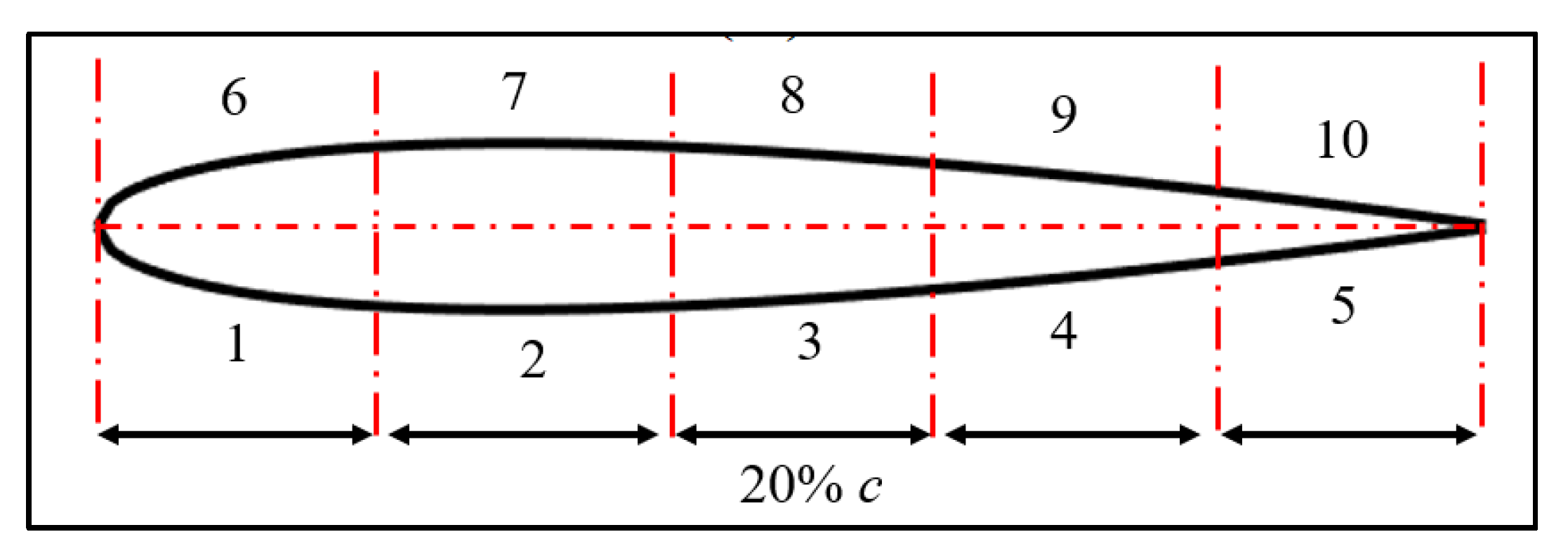
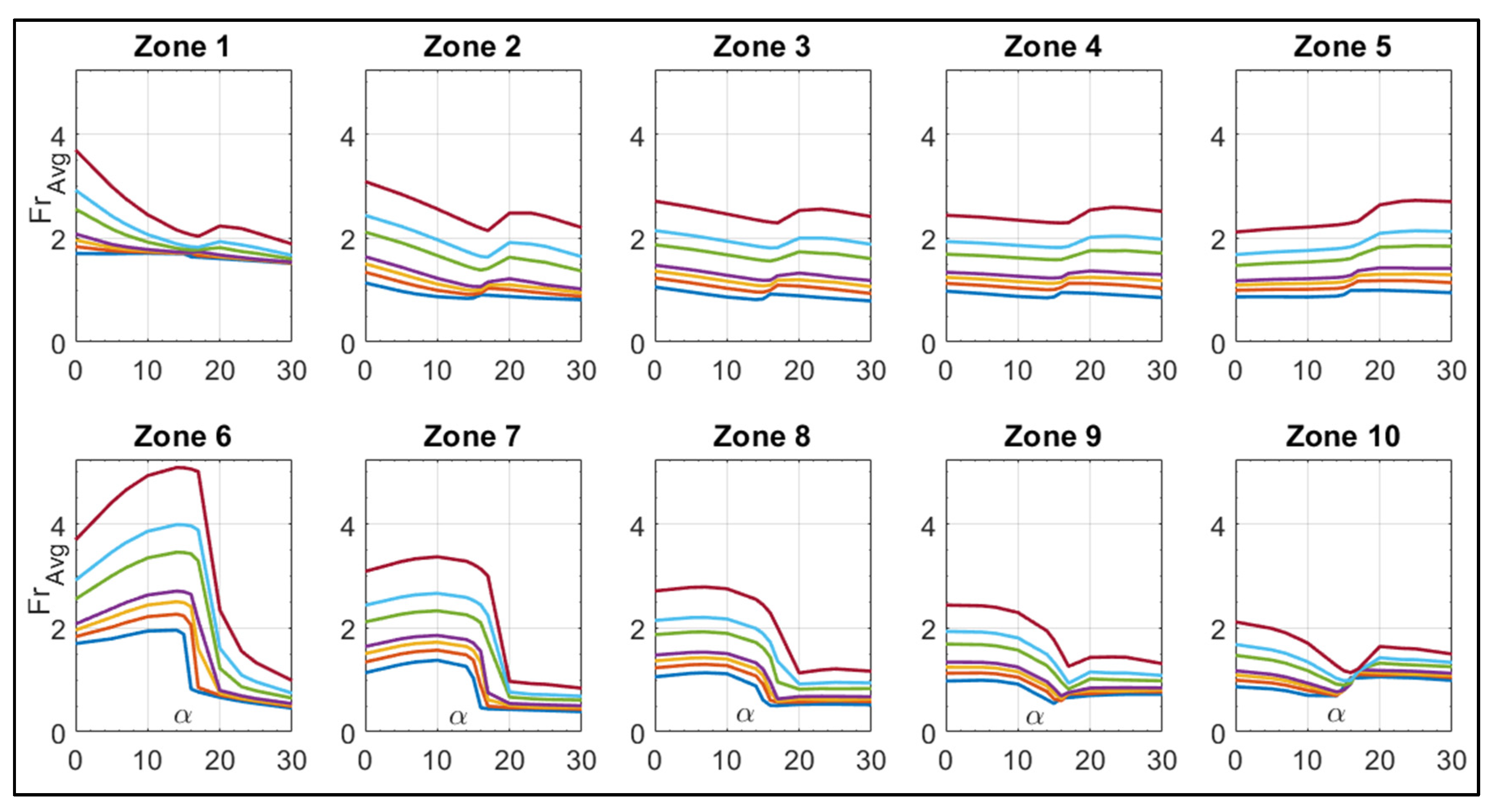
2.1.4. Zone with Maximum Fr

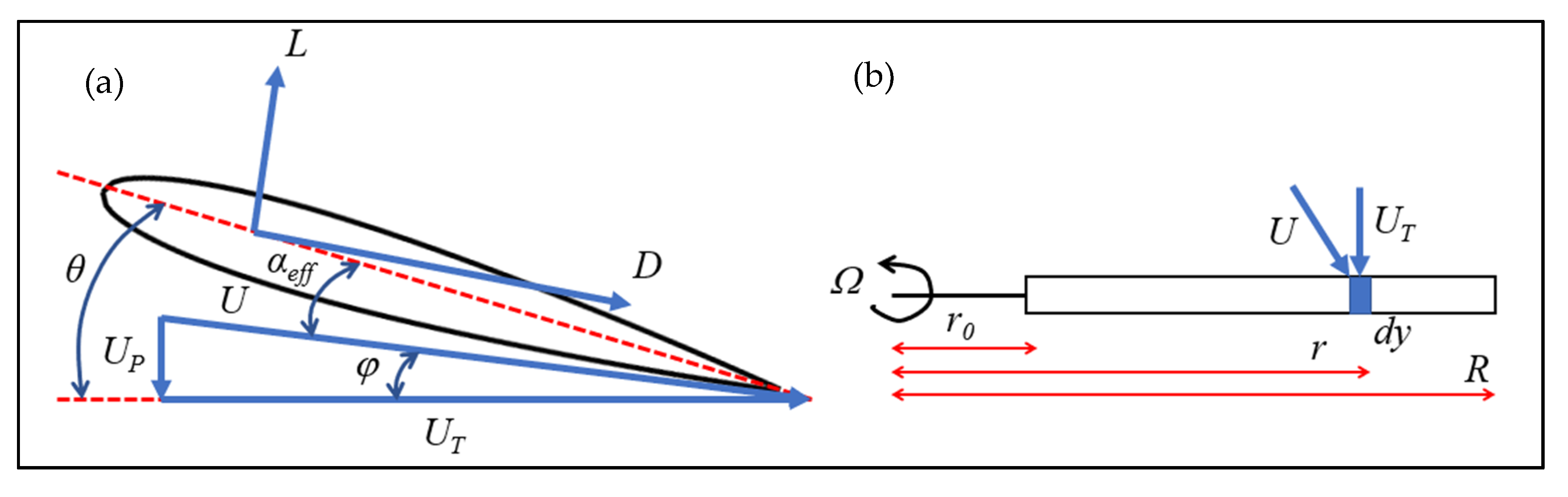
Calculating the average Fr over the NACA 0012 is useful to obtain an estimate of the overall convection. However, the movement of the stagnation point due to an increase in α will cause an increase of velocity on the pressure side of the airfoil and accordingly an increase of heat transfer. It is therefore important to determine the location of maximum heat transfer, or the zone that experiences the highest cooling rates and could be the most vulnerable for icing. Figure 2 shows a 10-zone division of the NACA 0012 wall. Each zone represents a specific length on the suction or pressure side of the airfoil and the length of each zone is equal to 20% of the chord. In a similar fashion of averaging the 512 datapoints from CFD over a single Fr value for a specific Re and α, the zone-specific average Fr is calculated and correlated into a similar form of Equation (2).

2.2. BEMT-RHT

The BEMT is a low-fidelity steady state approach to obtain rotor performance that can account for camber, twist, and different rotor configurations. However, it is of a steady state nature, does not represent the wake and the inviscid assumption eliminates viscous effects. This work uses a modified form of the classical BEMT (described in [33]) where viscous data from CFD are used and heat transfer on the rotor is calculated. Figure 3 shows the side and top view of a rotor blade with the respective loads and velocities. As the rotor spins with an angular velocity (Ω) at a specific pitch angle (θ), the lift (L) and drag (D) are created. The blade is divided into (n) segments between the tip radius (R) and root radius (r₀), each of equal length (dy). It is assumed that the resultant local flow velocity (U) at any blade element at a radial distance (r) from the rotational axis has an out-of-plane component (U_p) as a result of climb and induced velocities (V_c and v_i, respectively) as well as an in-plane component (U_T) (Equation (7)) because of the blade rotation with a relative inflow angle (φ). The inflow ratio and inflow angle are calculated by Equation (8), allowing the (α_eff) to be calculated by Equation (9) [33].

$$\begin{array}{ccc}{U}_P=V_c+v_i& U_T=\mathsf{\Omega }\times y& U=\sqrt{U_P^2+U_T^2}\end{array}$$

(7)

$$\begin{array}{cc}\lambda =\frac{V_c+v_i}{\mathsf{\Omega }R}=\phi r& \phi ={\tan }^{-1}\frac{U_P}{U_T}\end{array}$$

(8)

$${\alpha }_{eff}=\theta -\phi$$

(9)

To model tip vortex losses, a correction factor (f) is introduced, and an iterative solution is followed. The corrected form of the inflow velocity as well as the tip loss factor (F) are given in Equation (10) where (N) is the number of blades. The thrust and torque coefficients are finally calculated using Equation (11). In that equation, the torque coefficient is calculated by summing the incrementally induced and profile power coefficients (dC_Pi) and (dC_Po).

$$\begin{array}{ccc}F=\frac{2}{\pi }{\cos }^{-1}{e}^{-f}& f=\frac{N}{2}\left(\frac{1-r}{\phi r}\right)& \lambda (r_n)=\frac{\sigma C_{L\alpha }}{16F}\left(\sqrt{1+\frac{32F}{\sigma C_{L\alpha }}\theta (r_n)r_n}-1\right)\end{array}$$

(10)

$$\begin{array}{ccc}d{C}_T=4{\lambda }^2\left(r\right)rdr& d{C}_{P0}=\frac{1}{2}\sigma C_D{r}^{3}dr& d{C}_{Pi}=\alpha (r)\frac{d{C}_T}{dr}dr\end{array}$$

(11)

Table 1. Blade element momentum theory (BEMT)-rotor heat transfer (RHT) solution procedure.

		Without CFD Database	With CFD Database
BEMT	1	Guess a value for λ
	2	Calculate tip loss factor F
	3	Calculate αeff and φ (Equations (2) and (3))
	4	Redo until convergence (|λ i+1−λ i| = 10−5)
Aerodynamic Coefficients	5	Obtain CL-inv and CD-inv by a correlation	Obtain CL-visc and CD-visc from viscous database by interpolating αeff
Thrust and torque	6	Calculate incremental dCT, dCPi and dCPo, Output CT, CP and CQ
Heat transfer	7		For every Re and αeff at every r, calculate Fr

shows the classical and modified form of an iterative approach followed to solve the BEMT. Both approaches start with a guess on the inflow ratio (λ) followed by a calculation of F and φ. This is redone until a convergence criterion on λ is obtained (steps 1 to 4). At this step, the induced velocity v_i is determined based on the converged value of λ and by using Equation (8). Step 5 is to input C_L-inv and C_D-inv and for the classical approach, this is done by a simplified correlation of inviscid lift and drag. However, this work uses a viscous implementation of the BEMT where the converged α_eff from step 3 is used to interpolate viscous C_L-visc and C_D-visc from the CFD database. The thrust (C_T), torque (C_Q), and power (C_P) coefficients are then calculated in step 6. Finally, the novelty of the BEMT-RHT shows up in step 7 where the Re and α_eff are used to calculate Fr at every radial position using the CFD determined Fr correlations.

2.3. UVLM-RHT

The UVLM implementation of Katz and Plotkin [34] is adjusted in this work to enable rotor modeling. The method assumes an inviscid, irrotational, and incompressible flow around blades. Therefore, in its usual form, compressibility and separation effects cannot be modeled.

2.3.1. Discretization and Grid Construction

Figure 4 shows the vortex lattice distribution on a two-blade rotor. The blade geometry is described by (Root_X) and (Root_Y), as the spacing between the blade and the center of rotation in the x and y directions. (Ψ) is the azimuth angle traveled during the timestep (Δt). The lattices are placed on the blades’ camber line forming the corner points (Q_F), the leading segment of the lattice is placed on the panel’s 1/4 chord line, and the collocation point (Q_C) is at the center of the 3/4 chord line where the normal vector n is defined. At each timestep, a new row of shed wake elements is created and defined by its corner points (Q_W). The collocation point of each Q_W is placed at a distance equal to 0.3 × V_∞ × Δt. The UVLM assumes that the wake produced by the blades is force free and is therefore free to move with local stream velocity. This local velocity is a result of the induced velocity components by the blades as well as the wake itself. The strength of each new shed wake panel is set equal to that of the trailing edge in the previous timestep as in Equation (12) according to the Helmholtz theorem.

$${\mathsf{\Gamma }}_W\left(t\right)={\mathsf{\Gamma }}_{T.E.}\left(t-1\right)$$

(12)

2.3.2. Induced Velocities Calculation

Typically, the Biot–Savart law is used to calculate the velocity induced by the vortex segments. If the vortex segment points extend from point 1 to point 2, then the velocity induced on an arbitrary point P (${\overrightarrow{u}}_{1,2}$) is calculated using Equation (13). ${\overrightarrow{r}}_1\times {\overrightarrow{r}}_2$ is the product of the vectors extending from point P to points 1 and 2. ${\left|{\overrightarrow{r}}_1\times {\overrightarrow{r}}_2\right|}^2$ is the absolute value of the vector product, whereas $r_1$ and $r_2$ are the distances. Similarly, ${\overrightarrow{r}}_0\cdot {\overrightarrow{r}}_1$ and ${\overrightarrow{r}}_0\cdot {\overrightarrow{r}}_2$ represent the dot product. More details on the vector calculations can be found in [34].

$${\overrightarrow{u}}_{1,2}=\frac{\mathsf{\Gamma }}{4\pi }\frac{{\overrightarrow{r}}_1\times {\overrightarrow{r}}_2}{{\left|{\overrightarrow{r}}_1\times {\overrightarrow{r}}_2\right|}^2}{\overrightarrow{r}}_0\cdot \left(\frac{{\overrightarrow{r}}_1}{r_1}-\frac{{\overrightarrow{r}}_2}{r_2}\right)$$

(13)

The disadvantage of this approach is the presence of a singularity point when $\overrightarrow{r}$ ≈ 0, such as when the blade interacts with the wake. The Lamb–Oseen viscous correction model [35] solves the singularity using Equation (14) where the Oseen parameter is (ξ) = 1.25643, (r_c) is the core size radius, (a₁) = 10⁻⁴, and (r_o) is the initial core size [21]. (Γ) is the strength of the vortex segment and (ν) is the kinematic viscosity of air.

$$\begin{array}{cc}\overrightarrow{u}=\frac{\mathsf{\Gamma }}{4\pi }\frac{{\overrightarrow{r}}_1\times {\overrightarrow{r}}_2}{\left|{\overrightarrow{r}}_1\times {\overrightarrow{r}}_2\right|}{\overrightarrow{r}}_0\left(\frac{{\overrightarrow{r}}_1}{\left|{\overrightarrow{r}}_1\right|}-\frac{{\overrightarrow{r}}_2}{\left|{\overrightarrow{r}}_2\right|}\right)\left(1-e^{-\xi {\left(\frac{\left|{\overrightarrow{r}}_1\times {\overrightarrow{r}}_2\right|}{\left|{\overrightarrow{r}}_0\right|r_c}\right)}^2}\right)& r_c=\sqrt{r_0^2+4\xi \left(1+a_1\frac{\mathsf{\Gamma }}{\nu }\right)\nu \times \Delta t}\end{array}$$

(14)

2.3.3. Vortex Strength and Forces Calculation

For a two-blade rotor, the influence of the blade panels is stored in the (A) matrix (at the first timestep) comprising the influence of the first and second blade (first two terms on right-hand side of Equation (15)) as well as their mirror images (second two terms) to account for ground effects. K = 1 → L and L = IB × JB (IB and JB are the chordwise and spanwise number of lattices, respectively).

$$A_{K,L}={\left(u,v,w\right)}_{K,L}\cdot n_K+{\left(u_A,v_A,w_A\right)}_{K,L}\cdot n_K+{\left(u,v,-w\right)}_{K,L}\cdot n_K+{\left(u_A,v_A,-w_A\right)}_{K,L}\cdot n_K$$

(15)

The Right-Hand-Side matrix RHS is formed by enforcing the zero normal velocity boundary condition on the surface of the blade as shown in Equation (16). The (U(t)), (V(t)), and (W(t)) terms are the time-dependent kinematic velocity components whereas the (u_w), (v_w), and (w_w) terms are the induced velocity components due to the wake lattices. (n_K) is the normal vector to the surface of each blade lattice and the circulation of the blade lattices (Γ_K) is calculated by solving Equation (17).

$$RH{S}_K=-{\left[U(t)+u_W,V(t)+v_W,W(t)+w_W\right]}_K\cdot n_K$$

(16)

$${\mathsf{\Gamma }}_K={\displaystyle \sum _{L=1}^m{A}_{K,L}^{-1}}\times RH{S}_K$$

(17)

To account for compressibility effects, Glauert [36] proposed a compressibility correction (β) on high subsonic Mach numbers to include the compressibility effects in the calculations of VLM methods [10]. It is known as the Prandtl–Glauert compressibility correction factor. In particular, β is introduced to the calculation of the circulation as shown in Equation (18).

$$\begin{array}{cc}\beta =\sqrt{1-M{a}_K^2}& {\mathsf{\Gamma }}_K=\frac{1}{\beta }\times {\mathsf{\Gamma }}_K\end{array}$$

(18)

Finally, for the pressure distribution calculations the local circulation is needed so that the fluid dynamic loads can be computed using the Bernoulli equation. The pressure difference and force contribution in the body’s three axes are then given by Equations (19) and (20), respectively. (Δb), (Δc), and (ΔS) are the spanwise and chordwise lengths as well as the area of each lattice respectively.

$$\Delta p_{i,j}=\rho \left\{{\left[U(t)+u_W,V(t)+v_W,W(t)+w_W\right]}_{i,j}\cdot \left[{\tau }_i\frac{{\mathsf{\Gamma }}_{i,j}-{\mathsf{\Gamma }}_{i-1,j}}{\Delta c_{i,j}}+{\tau }_j\frac{{\mathsf{\Gamma }}_{i,j}-{\mathsf{\Gamma }}_{i,j-1}}{\Delta b_{i,j}}\right]+\frac{\partial }{\partial t}\mathsf{\Gamma }\right\}$$

(19)

$$\Delta F=-{\left(\Delta p\Delta S\right)}_{i,j}\cdot n_{i,j}$$

(20)

2.3.4. Slow Start Method

For free-wake calculations on rotor blades starting from rest, nonphysical instabilities of the initial wake are present. The root velocity influence is larger than the downward velocity and this will cause the strong root-vortex circulation to move upwards. A slow-starting method is used to overcome and avoid large fluctuations of simulation results [18]. The angular velocity of the rotor is increased linearly during a specified initial number of rotations as described in Equation (21) where (N_SS) is the slow-starting number of revolutions and (N) is number of revolutions traveled.

$${\mathsf{\Omega }}_{SS}=\mathsf{\Omega }\times \frac{N}{N_{SS}}$$

(21)

2.3.5. Modified Viscous-Heat Transfer Coupling Algorithm

In order to successfully link the UVLM to the CFD database, the α_eff needs to be obtained at each radial section. Different methods exist such as the Γ method or the α method [8], but the α method was favored since it can provide results even in post-stall angles [10]. The approach follows an iterative procedure between the inviscid C_L-inv (obtained using UVLM) and the viscous C_L-visc (obtained using CFD simulations) at each blade section as follows, where ($C_{L_{\alpha }}$) is the viscous lift curve slope, (α_Geo) is the geometric angle of attack, and the convergence criterion is (ε) = 0.001 [8]. This way, the Re and α_eff are determined at each radial position of the blade.

• Calculate α_eff at each blade section ${\alpha }_{eff}=\frac{C_{L-inv}}{C_{L_{\alpha }}}-\mathsf{\Delta }{\alpha }_{visc}+{\alpha }_{Geo}$.
• Find C_L-visc by interpolating α_eff in the CFD viscous database
• Check $\{\begin{array}{c}\begin{array}{cc}\left|C_{L-inv}-C_{L-visc}\right|<\epsilon & \begin{array}{cc}\to & {\alpha }_{eff}\end{array}\end{array}\\ \begin{array}{cc}\left|C_{L-inv}-C_{L-visc}\right|>\epsilon & \begin{array}{cc}\to & \Delta {\alpha }_{eff}=\Delta {\alpha }_{eff}+\frac{C_{L-visc}-C_{L-inv}}{C_{L_{\alpha }}}\end{array}\end{array}\end{array}$
• Adjust α_eff in the first step by the found Δα_visc
• Repeat until |C_L-inv − C_L-visc| < ε

2.3.6. Complete UVLM-RHT Solution Procedure

This section summarizes the complete solution procedure followed by the UVLM-RHT.

Table 2. Unsteady vortex lattice method (UVLM)-RHT solution procedure.

	Step	Task
UVLM	1	Blade camber line geometry and flight path kinematics
	2	Blade influence coefficients matrix A
	3	Form the right-hand side matrix RHS
	4	Solve RHS to obtain Γ
	5	Pressure and forces calculation (CT, CLy, …)
	6	Wake rollup
Heat transfer	7	Viscous coupling algorithm (Re, CL-visc, and αeff)
	8	For every Re and αeff at every collocation point, calculate Fr

shows the steps followed to calculate the forces and heat transfer on the rotor. Steps 1 to 6 are based on the classical application of the UVLM, with the addition of the slow start, the Lamb–Oseen viscous correction, and the Prandtl–Glauert compressibility correction. The originality of the present work shows up in the last two steps. Step 7 applies the viscous coupling algorithm presented in Section 2.3.5, whereas step 8 uses the Re and converged α_eff at each radial position to calculate the Fr based on the CFD determined correlations. Steps 3 to 8 are then repeated for each timestep until the Fr on all the radial and azimuthal locations of the blades is obtained.

3. Results

In this section, the results of the laid out methodologies are presented. For the CFD part of this work, the test case of the flat plate is compared to heat transfer correlations as well as other implementations of the S-A turbulence model from the literature. Next, the Fr_Avg and Fr_Max calculated for the NACA 0012 for each simulation are presented along with the respective final form of the correlation of each. For the implemented BEMT and UVLM, four experimental test cases are chosen to validate the aerodynamic tools corresponding to rotors in hover, axial, forward flight as well as in ground effect. Finally, the novel implementation of the BEMT-RHT and UVLM-RHT is used on a modified Bell 429 tail rotor to calculate the blade heat transfer in various flight modes.

3.1. CFD Heat Transfer Results

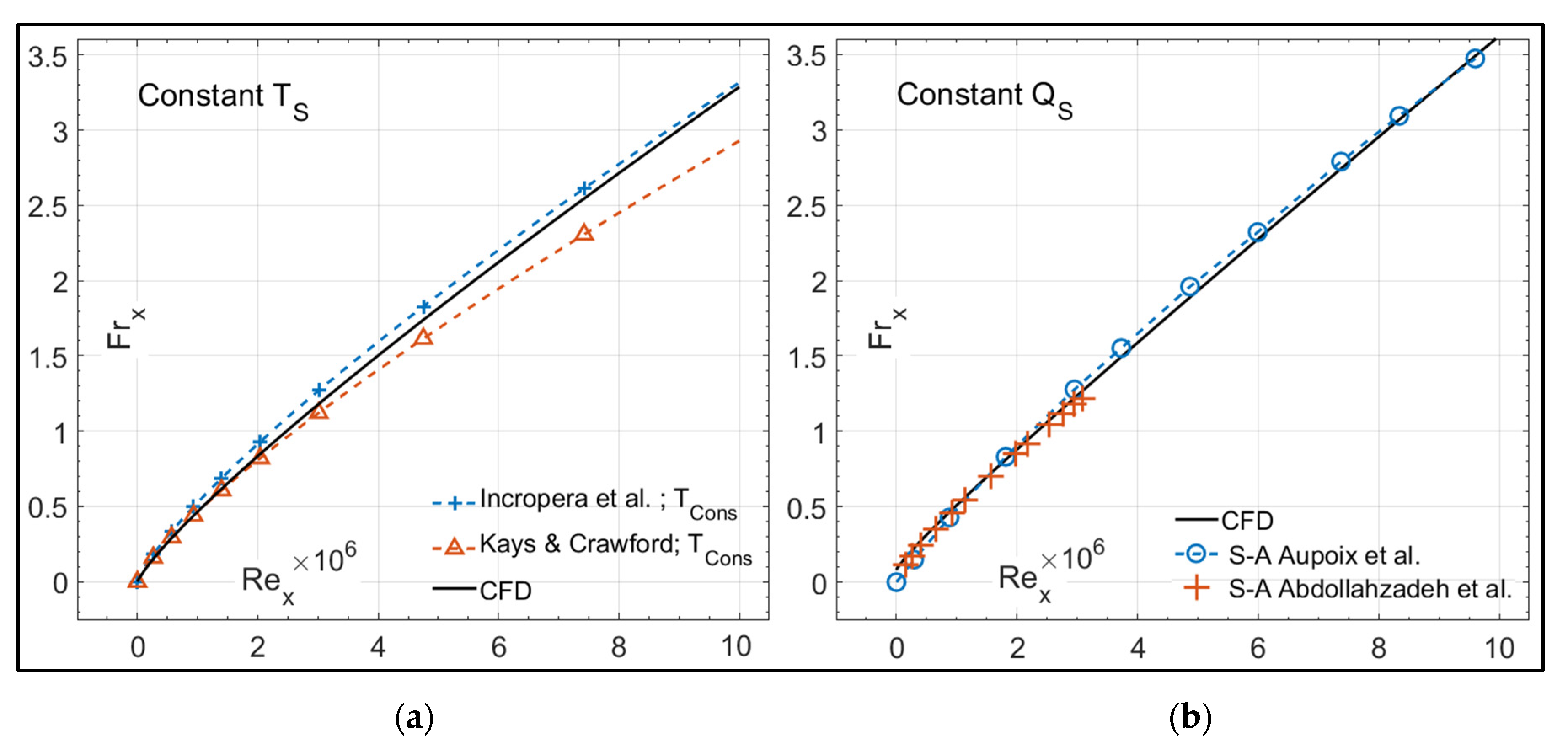
3.1.1. Flat Plate Verification Test Case

To verify the results of this work’s CFD thermal simulations, the correlations for the local Nusselt number (Nu_x) on a flat plate, under turbulent flow conditions, and a constant T_S boundary condition, are picked from previous studies (see [32]). Each source provides a correlation for the Nu_x as shown in

Table 3. Flat plate correlations and data compared with CFD for different B.C. S-A: Spalart–Allmaras.

Constant Surface Temperature TS	Constant Surface Heat Flux QS
$N{u}_x=0.0287\times {\mathrm{Re}}_x^{0.8}\times {\mathrm{Pr}}^{0.6}$ [32]	S-A CFD data, Aupoix et al. [37]
$N{u}_x=0.0296\times {\mathrm{Re}}_x^{0.8}\times {\mathrm{Pr}}^{0.334}$ [28]	S-A CFD data, Abdollahzadeh et al. [29]

. The Nu_x is transformed into the Fr_x by $F{r}_x=N{u}_x/\sqrt{R{e}_L}$, where (Re_L) is the Re based on the total length of the plate. As for the comparison with literature implementations of the S-A turbulence model for heat transfer prediction, the numerical results of Aupoix and Spalart [37] and Abdollahzadeh et al. [29] are chosen. Both provided the local Stanton number (St_x) for a flat plate with a constant Q_S B.C. The St_x is transformed into the Fr_x by $F{r}_x=\left(S{t}_x\times R{e}_x\times Pr\right)/\sqrt{R{e}_L}$. In this work, each B.C. is simulated using CFD and the computational details described in Section 2.1.2. The results of the comparisons are shown in Figure 5.

Figure 5 shows the variation of the Fr_x versus the Re_x across the flat plate. The subfigure on the left represents the variation for a constant T_S whereas the constant Q_S B.C. is on the right. For either B.C. the Fr_x increases across the plate due to a direct increase of the Re_x. For the case of constant T_S, the discrepancy between the results of CFD and the correlation of Incropera et al. is around 7% for all Re_x. The discrepancy compared to the Kays and Crawford correlation is around 7% for Re_x < 5 × 10⁶ and 12% for Re_x > 5 × 10⁶. It should be noted that both correlations claim an accuracy within 15%, so the discrepancy found with CFD results is satisfactory. For the constant Q_S, the S-A implementation of this work as well as those from the literature all provide very similar results with no more than 2% discrepancy, mainly due to the different discretization of each numerical implementation.

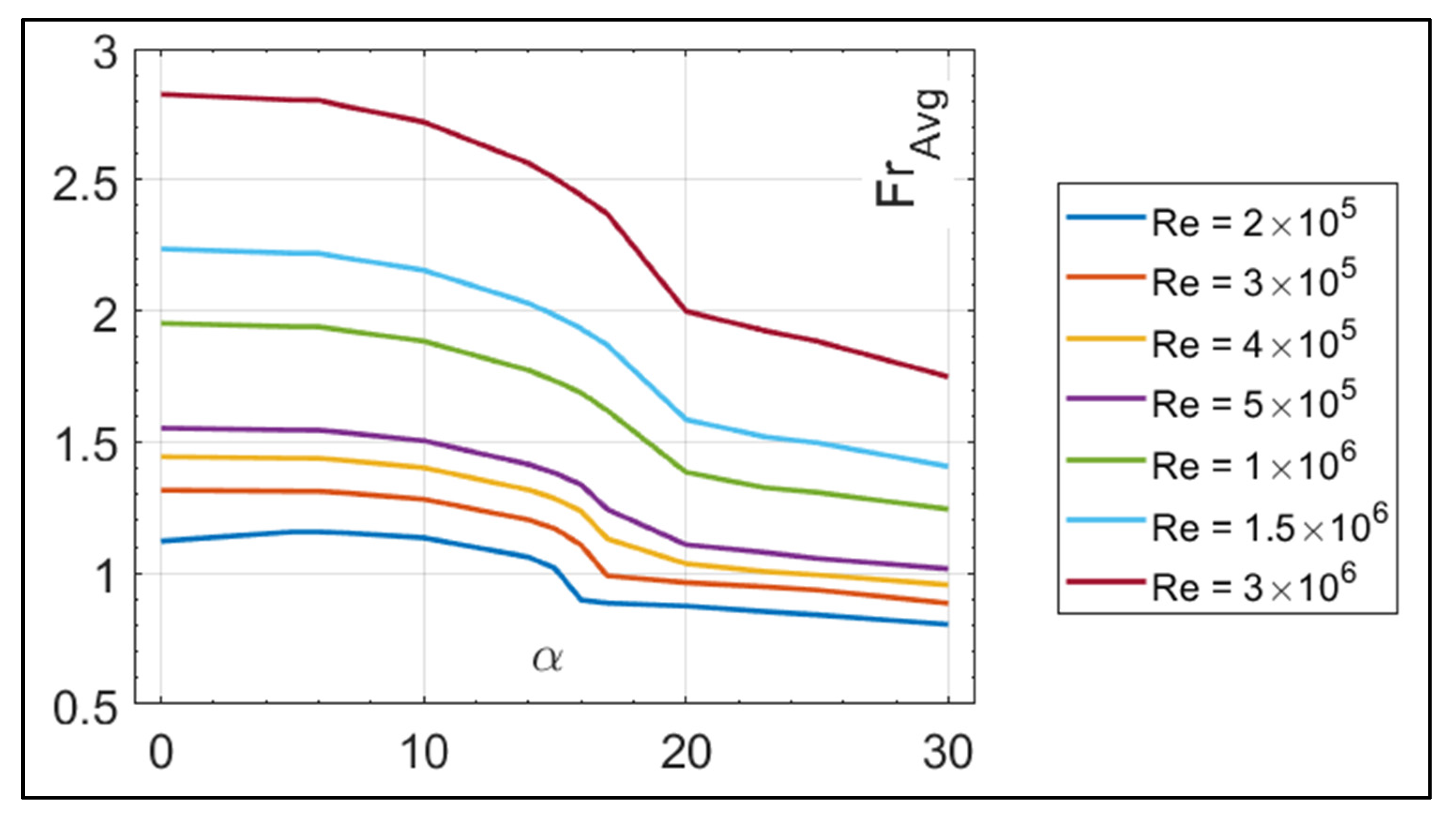
3.1.2. Average Frossling Number Correlation

For the NACA 0012 CFD simulations, the methodology described in Section 2.1.3. produces a specific average Fr value for each simulated Re and α. Figure 6 shows the variation of the average Fr obtained for all simulations for different Re and α. Higher Re directly increased the values of Fr and an increase of α caused a decline in Fr starting from α = 0°.

These data were used to build an average Fr correlation for the NACA 0012 (for a constant T_S B.C. and a fully turbulent flow) in the proposed form of Equation (22) (α is in rad) where A, B, C, and m are parameters determined based on a curve fitting method [38], the average discrepancy between the Fr values determined from CFD simulations and those calculated with the correlation is 3.2%. This leads to a simplified application of Equation (22) in the BEMT or UVLM where only the Re and α_eff are needed to promote these aerodynamic methods into heat transfer prediction tools.

$$\begin{array}{cc}F{r}_{Avg}=A\left(1+B\times \alpha +C\times {\alpha }^2\right)R{e}^{m}P{r}^{1/3}& \{\begin{array}{ccc}A=0.023& C=-0.678& 2\times {10}^5\le Re\le 3\times {10}^6\\ B=-0.389& m=0.330& 0^{\circ }\le \alpha \le {30}^{\circ }\end{array}\end{array}$$

(22)

3.1.3. Maximum Frossling Number Correlation

As a further step from the previous section, this section examines the location of the maximum heat transfer on the wall of the NACA 0012. The methodology of Section 2.1.3. was applied on each of the considered 10 zones in Figure 2. Figure 7 shows the average Fr for each of the 10 zones. For each zone, the Fr is plotted as a product of variation of Re and α. The colors used to represent the different Re in Figure 7 are the same ones in Figure 6. Zone 6 shows the highest Fr for all Re, specifically at α < 16°. In a similar way to how the correlation for the Fr_Avg was obtained, the data for zone 6 in Figure 7 were used to produce a correlation for the Fr_Max as shown in Equation (23). A, B, C, and m are parameters were determined using a curve fitting method, and the average discrepancy was 0.5%.

$$\begin{array}{cc}F{r}_{Max}=A\left(1+B\times \alpha +C\times {\alpha }^2\right){\mathrm{Re}}^m{\mathrm{Pr}}^{1/3}& \{\begin{array}{ccc}A=0.0112& C=-11.489& 2\times {10}^5<\mathrm{Re}<3\times {10}^6\\ B=3.678& m=0.4033& \alpha <{16}^{\circ }\end{array}\end{array}$$

(23)

3.2. Validation of Implemented BEMT and UVLM

This section serves to validate the numerical tools developed based on the BEMT and UVLM. The first section compares the hovering rotor thrust prediction by the BEMT and UVLM to the results of the UVLM implementation of Colmenares et al. [17] and Ferlisi [19], as well as the experimental results for the thrust and sectional lift coefficient (C_Ly) of the work of Caradonna and Tung [39]. The other section uses the four-blade experimental results of the Lynx tail rotor setup [40] in ground effect to validate the locations of the wake tip vortices predicted by the UVLM as well as a comparison to the experimental thrust estimate and the numerical method of Cheeseman and Bennett [41]. Next, the axial flight modeling is validated by comparing the wake tip vortices positions predicted by the UVLM to experimental data by Caradonna [42] at different climb ratios. The figure of merit (FM) predicted by the UVLM and BEMT of this work is also compared to that of the experiments as well as the UVLM implementation of Ferlisi [19]. Finally, the UVLM in forward flight is validated by comparing the sectional thrust coefficient predicted to the results of the AH-1G rotor experimental test case [43] and the numerical results of previous studies [44,45].

3.2.1. Two-Blade Hovering Rotor

The experimental setup consists of two hovering blades having a NACA 0012 airfoil section spinning at Ω = 1250 rpm with Ma_Tip = 0.43. The chord is 0.1905 m (equal to the root cut-out radius) with a radius of 1.143 m, and three difference pitch angles are used (5°, 8°, 12°). The BEMT was run using n = 200 radial sections to predict the steady state value of C_T. For the UVLM, the test case was run for 24 revolutions for ΔΨ = 15° using 10 × 25 vortex panels on each blade and the first two rotor revolutions were used to slow-start the rotor. The presented UVLM data are the ones at the 23rd simulated revolution, when the C_T and C_Ly are stabilized and do not change between timesteps. Figure 8 shows the comparison between the results of the UVLM, BEMT, and the literature. The left side shows the variation of C_T as a function of the rotor revolutions for θ = 5°, 8°, and 12° obtained using the viscous UVLM and BEMT compared to results of Colmenares et al. [17]. The right side shows the variation of the C_Ly recorded by the experiment along the length of the blade versus the viscous UVLM and BEMT at the three different θ.

For the BEMT, the steady state C_T is overpredicted by around 15–20% for all θ, mainly due to the simplified calculations method of the induced velocities. As for the UVLM, the rotor thrust increases from 0 just when the blades commence movement, reaches a maximum at the second revolution (where maximum speed is reached), and then exhibits a fluctuating behavior (± 4%) around an averaged C_T value. The average C_T predicted by the UVLM and BEMT is compared to other numerical tools and the experiment in

Table 4. Average C_T predictions by different numerical methods versus experimental values.

	UVLM	BEMT	Ferlisi	Colmenares et al.	Caradonna and Tung
θ = 5°	0.00243	0.00290	0.00237	0.00221	0.00213
θ = 8°	0.00477	0.00540	0.00460	0.00467	0.00459
θ = 12°	0.00794	0.00910	0.00824	0.00821	0.00796

, and it is concluded that the UVLM agrees better with the literature results (5% discrepancy), whereas the BEMT overpredicts all other estimations by almost 20%. As for the C_Ly, the UVLM agrees within 2% of experimental data whereas the BEMT also shows an overestimation of around 20%. With that in mind, it is suspected that the α_eff predicted by UVLM may also be closer to that of the experiment, although no such data exist to compare with.

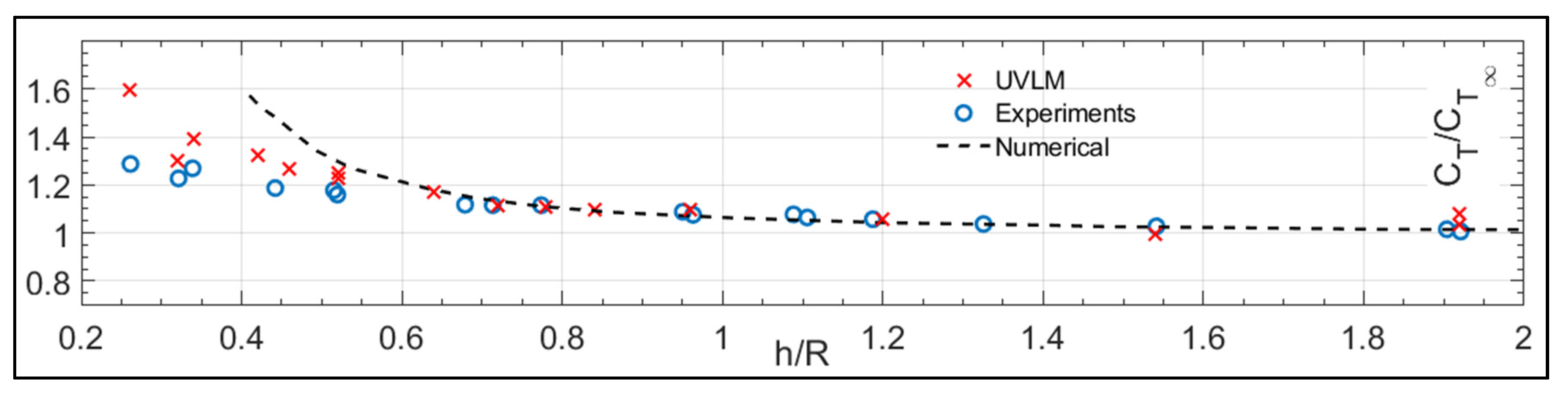
3.2.2. Four-Blade Hovering Rotor in Ground Effect

The Lynx tail rotor experimental setup [40] used a four-blade hovering, vertically mounted, rotor with a 0.18 m chord and a 1.108 m total radius (0.425 m root cut) near the ground. The rotor was spinning at 1660 rpm and had an NPL 9615 airfoil shape. For every ground clearance ratio (h/R), a set of θ was used to form a test case and the C_T was measured. Four of these tests used a shadowgraph to capture the trailing wake in the axial and radial directions. The BEMT is not implemented here since it does not provide a wake shape nor is capable of modeling the ground effect. Figure 9 shows the results of the tip vortices axial location (TVAL) and tip vortices radial location (TVRL) obtained by UVLM compared to those of the experiments.

The TVAL and TVRL are non-dimensional parameters that describe the location of the shed wake vortex as the rotor is spinning and are calculated according to Equation (24). They are measured in terms of the wake age that represents the azimuth angle by which the blade rotated since a specific wake element was shed.

$$\begin{array}{cc}TVAL=\frac{Q_{W_z}\left(\mathsf{\Psi }\right)}{R_{Tip}}& TVRL=\frac{Q_{W_x}\left(\mathsf{\Psi }\right)}{R_{Tip}}\end{array}$$

(24)

The subfigure on the upper left is for a test with no ground effect (h/R = ∞) and every other subfigure shows the tip locations for a test with a smaller h/R. The idea is to determine if the UVLM could be validated even at small h/R. For h/R = ∞ and h/R = 0.84, the axial and radial tip locations are captured with around 92% agreement. Discrepancies exist but the overall wake behavior is well captured. However, as the h/R is decreased to 0.52 and 0.32 respectively, the radial positions predicted by the UVLM fail to agree with the experimental data although the axial locations are well predicted.

For C_T predictions, Figure 10 shows the variation of the C_T versus h/R predicted by the UVLM compared to those recorded from the experiments. The predictions of the numerical method of Cheeseman and Bennett [41] are also presented to see the how the UVLM compares to other numerical calculations. Existence of two data points for the same h/R indicate a different θ for each.

For h/R ≥ 0.52, the UVLM predicts C_T values within 10% of the experimental and numerical results of the literature. The results from the UVLM are closer to the numerical values than they are to those of the experiments. In addition, both the UVLM and the numerical method of Cheeseman and Bennett fail to capture the C_T in extreme ground clearance (h/R ≤ 0.32), similar to the radial location predictions. It is believed that the failure of the implemented UVLM to model an extreme ground effect may have been either the results of discretization or the induced velocities calculations. It was observed that when the h/R was decreased, the wake lattices near the ground became very condensed and got much closer together. This may have resulted with the vortex segment distances being very small and the induced velocities not calculated properly. For the implemented UVLM in the work of Ferlisi, the comparison of the predicted TVRL actually matched the experimental results but his predicted TVAL failed to provide a good agreement.

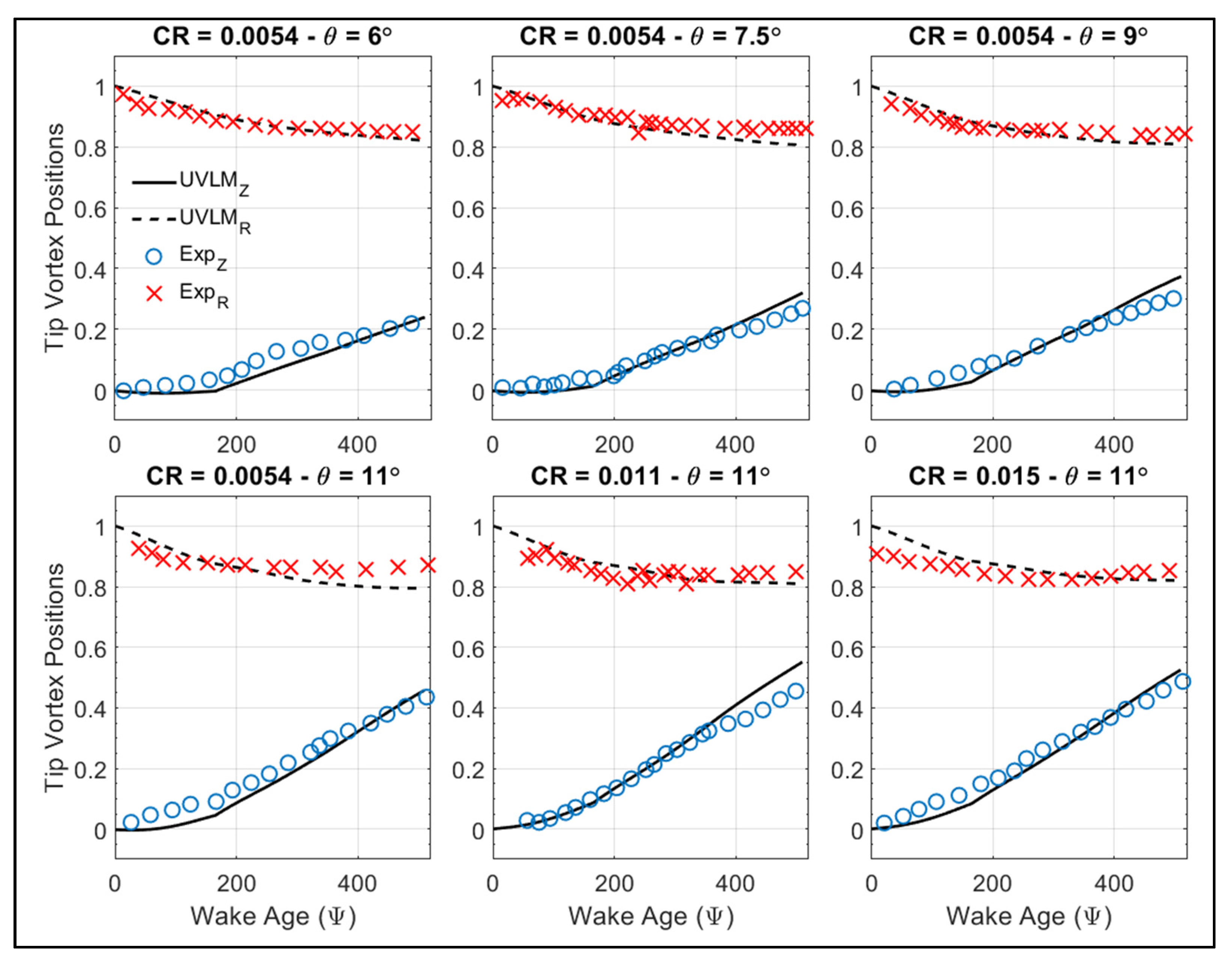
3.2.3. Two-Blade Rotor in Axial Flight

Caradonna’s [42] two-blade rotor experiment was analyzed for a rotor in axial flight. The rotor radius is 1.067 m and the aspect ratio is 13.67. The blades are not tapered nor twisted. The sectional airfoil is a symmetric Bell profile. The root cutout is approximately equal to one chord. The rotor speed is 1800 rpm, the Ma_Tip is around 0.46 and the climb ratios (CR) are varied. The goal in this section is to validate the wake shape and blade loading predicted by the UVLM, so the TVAL and TVRL predicted by the UVLM (using Equation (24)) are compared to the ones recorded by the experiments. The numerical model consists of 10 × 25 vortex lattices on each blade and was run for 24 revolutions with ΔΨ = 10°. Figure 11 shows the TVAL and TVRL obtained by the UVLM compared to those of the experiments for a length of 1.5 revolutions. The cases presented involve a rotor with θ = 6°, 7.5°, 9°, and 11° whereas CR = 0.0054, 0.011, and 0.015. The UVLM results were recorded at the 20th turn after a steady state wake shape was observed.

It can be seen from Figure 11 that the tip vortex locations predicted by the UVLM agree with those of the experiments within 90% although some discrepancies exist for the axial data in the test case of CR = 0.011. The implementation of the UVLM is therefore capable of producing the wake shape from the experiments. To validate the blade loading however, the FM is computed and shown in Figure 12. Results from the experiments as well as the viscous UVLM implementation of Ferlisi are used to validate the results from the UVLM and BEMT of this work. The viscous corrections of Ferlisi were obtained using XFOIL whereas this work uses CFD viscous corrections. This is done for 0.002 < CR < 0.04.

The results of Figure 12 show that the viscous BEMT and UVLM implemented in this work predicted the variation of the FM well compared to the numerical method from the literature as well as the experiments, with a discrepancy for CR < 0.005. The results of the BEMT and UVLM agree within ±7% of the experiments, a closer agreement than the method from the literature possibly due to higher order estimation of the viscous data from CFD compared to XFOIL. All the numerical methods shown in Figure 12 showed a discrepancy with the experiments for CR < 0.005. As explained by Caradonna, this may be due to experimental errors where a linear variation of FM down to CR = 0 is more likely expected.

3.2.4. Two-Blade Rotor in Forward Flight

The AH-1G 2-blade rotor experiment by Jeffrey [43] is also analyzed for a rotor in forward flight. The goal in this section is to validate the blade loading calculated by the UVLM for a rotor in forward flight. The rotor radius is 6.7 m and the aspect ratio is 9.2 with a linear twist ratio of −10°. The rotor operates at Ma_Tip = 0.68 and the advance ratio (AR) is 0.19. The numerically modeled blade with the UVLM consisted of 20 × 60 vortex lattices that ran for 10 revolutions at ΔΨ = 10°. The calculated sectional C_T is compared to the experiments, the unsteady potential method (PM) of Tan and Wang [44], the free wake method of Kim and colleagues [46], and the CFD calculations of Lee et al. [45].

Figure 13 shows the variation of C_T on the blade versus the wake age. Each subfigure corresponds to a radial section located at r/R = 0.87, r/R = 0.91, and r/R = 0.97. The results of the UVLM and those of the experiment are compared in every subfigure whereas the results of the numerical methods from the literature are shown as follows: the PM at r/R = 0.87, the free wake at r/R = 0.91, and CFD at r/R = 0.97, to avoid data overfill in the figures. The variation of the C_T versus Ψ corresponds with the movement of the blade from an advancing side to the retreating side. The point of minimum tip local velocity is at Ψ = 90° and the maximum velocity is reached half a revolution after at Ψ = 270°. Relating to Figure 13 and for all r/R shown, the C_T increases starting at Ψ = 90° to a maximum around Ψ = 270° before decreasing when the blade is retreating. This effect is captured well by the UVLM and all other shown data from the literature compared to the experimental results.

The UVLM agrees within 80% to the results of the experiments for all r/R. However, at r/R = 0.87, the discrepancy of the UVLM compared to the PM is around 20%. At r/R = 0.91, the UVLM shows discrepancy as low as 5% with the results of the free wake method from the literature before Ψ = 270° and around 20% for 270° < Ψ < 360°. The discrepancy with the CFD results at r/R = 0.97 is around 10% but the C_T is overpredicted at Ψ < 90°. The CFD results were the best in terms of numerical results mainly due to high fidelity approach and detailed calculations. Unlike the UVLM, the PM models the thickness of the blades, so this perhaps explains the better agreement with experimental results. The UVLM of this work behaved similarly to the other free wake method. The discrepancies between the two may be due to a different grid size and timestep used.

3.3. Rotor Heat Transfer Results

To present the results of the heat transfer distribution on a rotor using the BEMT-RHT and UVLM-RHT, a modified version of the Bell 429 tail rotor is chosen. For this work, the airfoil profile is considered to be a NACA 0012 to relate the calculations to the proposed Fr correlations and due to confidentiality purposes. The four-blade rotor has a chord of c = 0.1752 m with a diameter of 1.652 m. It operates at a speed of Ω = 2292 rpm with a Ma_Tip = 0.6 at hover. The blades are not twisted, and the simulated pitch angle is θ = 8°. The blade surfaces are assumed to be maintained at a constant T_S to match the boundary condition imposed on the 2D CFD simulations. The objective is to quantify the heat transfer predicted by the BEMT-RHT and the UVLM-RHT using the correlations for Fr_Avg and the Fr_Max in Equations (22) and (23) for basic rotor operations under typical flight conditions. The air properties were evaluated at a temperature T_∞ = 268.15 K.

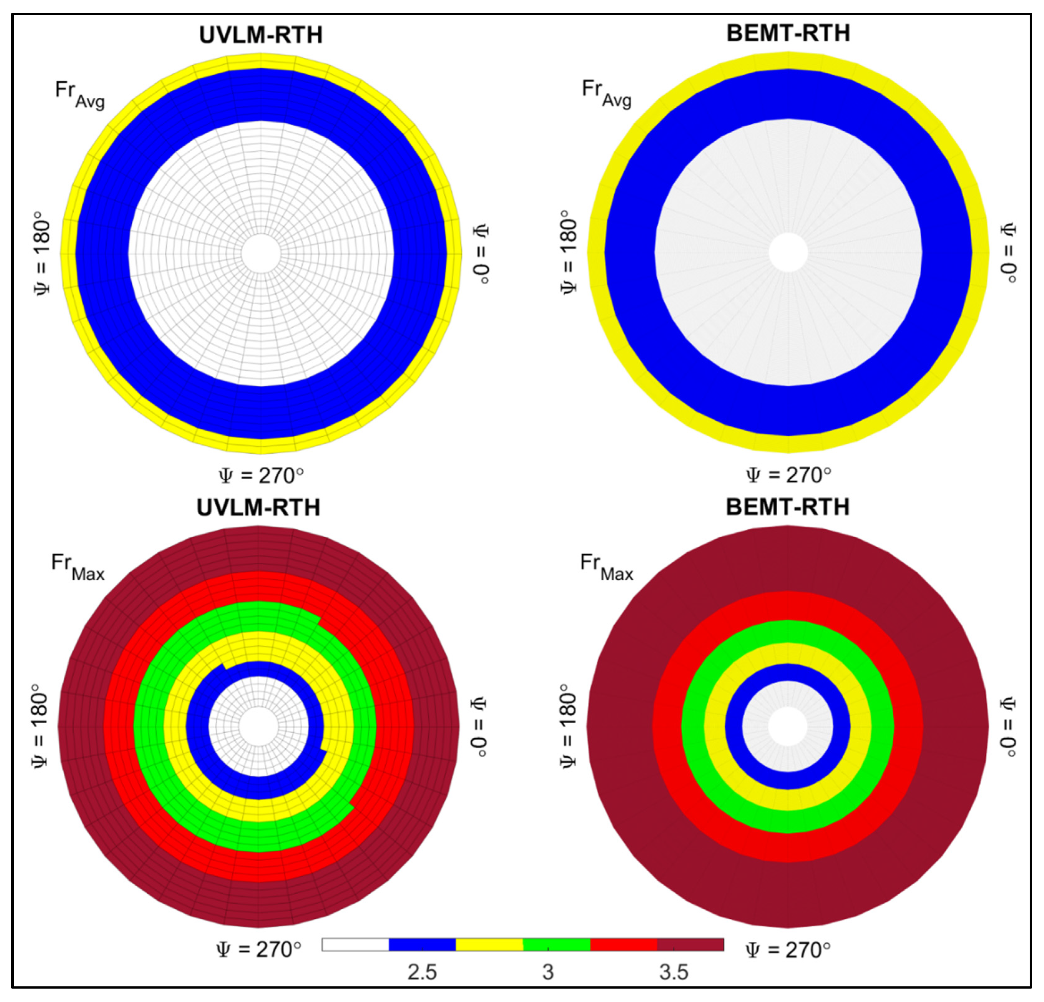
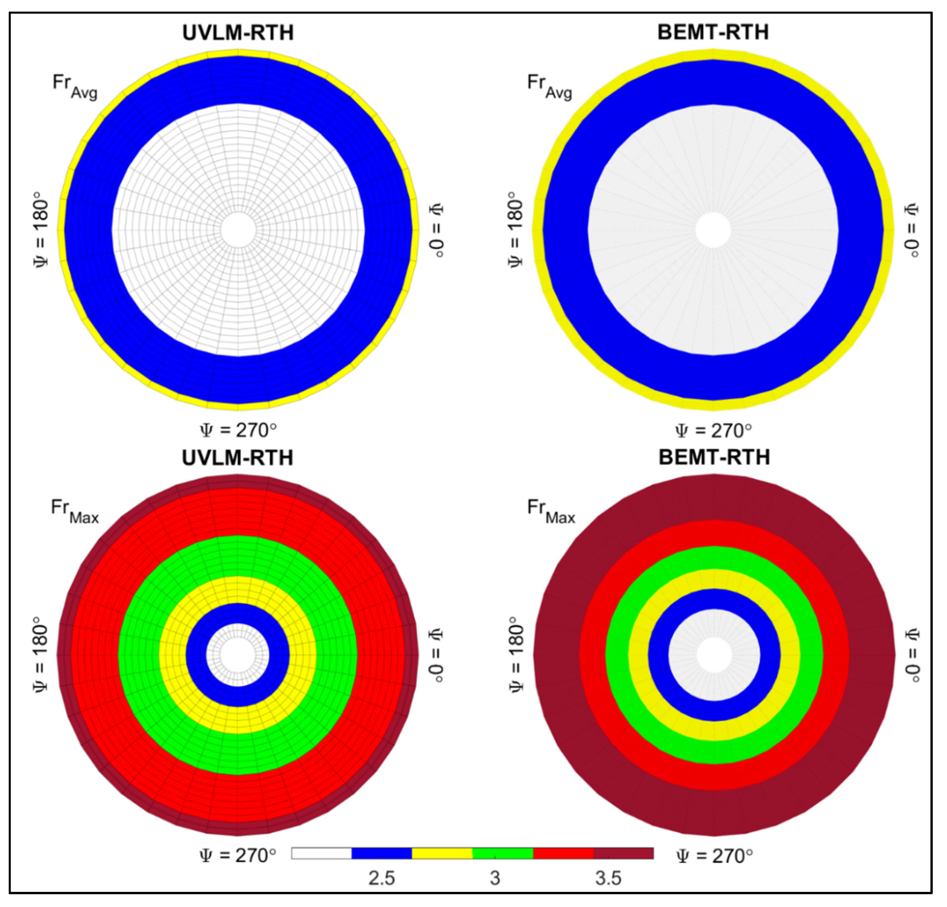
3.3.1. Hover Out of Ground Effect (OGE)

For the case of the hovering rotor, the velocity distribution as the rotor spins will only vary from hub to tip and will remain constant at any Ψ, thus the Re will vary only in the radial direction. To estimate the Fr on the rotor, the hovering test case was run using the UVLM-RHT with 10 × 25 vortex lattices at ΔΨ = 10° for a total of 20 revolutions. At the 20th revolution, the computed Re and α_eff at every radial position and at every blade ΔΨ from the UVLM were used to calculate the Fr_Avg and Fr_Max using the proposed correlations. The BEMT-RHT was used with n = 200 blade elements. The results of Re and α_eff are already in their steady state form with a single value corresponding to each blade element n. Equations (22) and (23) are again applied to obtain the Fr_Avg and Fr_Max across the blade length.

The solution from the UVLM is time dependent, but it was observed that steady state variations of the wake shape and thrust were attained after 20 revolutions as shown in Figure 14. In the figure, the wake contraction below the rotor plane is observed and the wake propagates in the negative Z axis direction freely without restriction, similar to results of Colmenares et al. [17]. The pure rotational movement of the rotor produces a symmetric wake. Eventually, the wake rolls up and an inverted mushroom shape is formed.

Figure 15 shows the contours of the steady state Fr_Avg and Fr_Max predicted by the BEMT-RHT and the UVLM-RHT for a steady state rotor revolution. The upper row of Figure 15 shows the results of the Fr_Avg for the UVLM and BEMT respectively, whereas the bottom row shows the Fr_Max in the same order. The predicted values by each method are symmetric across the rotation plane. In the upper left side of Figure 15, the predicted values of Fr_Avg from the UVLM-RHT vary between a minimum of 1.4 near the hub and a maximum of 2.7 on the tip. This is associated with the linear variation of the Re from hub to tip and indicates that the computed α_eff had no significant impact on results. A similar conclusion may be drawn by the examining the predicted Fr_Max of the UVLM-RHT that varied between 1.9 and 3.8 from hub to tip (32% and 27% higher than Fr_Avg).

The results of the BEMT-RHT showed excellent agreement with those of the UVLM-RHT. Comparing the values from the right side of Figure 15 to those on the left side, it is found that the discrepancy in Fr_Avg is no more than 4% with the BEMT-RHT underestimating the UVLM-RHT. A slightly higher discrepancy was seen for the Fr_Max predictions at around 11% overestimation by the BEMT-RHT. For the test case of the hovering rotor, the Re calculated by the two methods was the same but the predicted α_eff by the BEMT-RHT was higher than that of the UVLM-RHT.

3.3.2. Hover in Ground Effect (IGE)

To understand the changes on blade heat transfer prediction for a rotor close to an obstacle, the Fr_Avg and Fr_Max predicted by the UVLM-RHT in ground effect are investigated in this section. The implementation of the BEMT in this work cannot account for the ground. The same hovering test case of the modified Bell 429 tail rotor is modeled but with a ground clearance h/R = 1 to avoid failure in extreme ground effect, based on the validation test case of Section 3.2.2. The UVLM-RHT was run with 10 × 25 vortex lattices at ΔΨ = 10° and 2.5 slow-start revolutions for a total of 20 revolutions. Similar to the hovering test case, the computed Re and α_eff at every radial position of the 20 revolutions were used to calculate the Fr_Avg and the Fr_Max using Equations (22) and (23).

Figure 16 shows the wake shape obtained by the UVLM-RHT for the four-blade rotor near the ground after 20 revolutions. It is seen that the symmetry of the wake propagation is conserved and agrees with the results of Ferlisi [19]. However, due to the limited ground clearance below the rotor plane, the wake was seen to stop propagating at Z = 0 (where the rotor is at Z = h/R = 1) and expanded in the X and Y directions while still rolling up into a flattened inverted mushroom shape. A notable difference with the case of the hovering OGE rotor was the greater expansion of the hub wake lattices. Near the hub of the rotor, the wake lattices grew more than their counterparts when no ground was modeled.

Figure 17 shows the contours of the predicted steady state Fr. The Fr_Avg values are shown on the left-hand contour and the contour on the right represents the Fr_Max. Near the hub, the values are found at a minimum of 1.6 and a maximum of 2.75 near the tips for the Fr_Avg and between 2.2 and 3.9 for the Fr_Max (27% and 29% higher, respectively). By comparing the results from the hovering test case, the predicted Fr_Avg and Fr_Max at h/R = 1 are almost 8% different than their counterparts at h/R = ∞. Since the Re is the same whether a ground effect is present or not, it is concluded that the wake proximity to the ground will cause the α_eff to increase and to cause disturbances in the heat transfer across the plane of rotation. This was confirmed by comparing the α_eff predicted for each case, translated by the decrease of the Fr_Avg and increase of the Fr_Max compared to the hovering OGE test case.

3.3.3. Axial Flight

The axial flight for a horizontally mounted rotor corresponds to lateral maneuver of a vertically mounted tail rotor. In both cases, there exists a velocity component perpendicular to the rotor plane causing a drop in the local blade velocity. The climb ratio is used to determine the ratio of climb velocity V_∝ to the tip speed of the rotor Ω × R_Tip. In this section, the modified Bell 429 tail rotor is modeled with CR = 5%. The UVLM-RHT was run with 10 × 25 vortex lattices at ΔΨ = 10° for a total of 20 revolutions. The BEMT-RHT calculations were done with n = 200 blade elements and converged in less than two minutes.

Figure 18 shows the wake shape produced by the UVLM-RHT for the 4-blade rotor in axial flight, similar to the one in [42]. The rotor starts from Z = 0 and travels upwards due to the indicated V_∝. The root vortices are entirely pushed below the rotor plane. As the rotor is climbing, wake elements are produced and shed from the T.E. of the rotating blades. The combination of the axial and rotational velocities causes the wake to be elongated yet preserve its contraction and symmetry.

Figure 19 shows the contours of the steady state Fr_Avg and Fr_Max predicted by the BEMT-RHT and the UVLM-RHT for the rotor in axial flight. A symmetric profile of Fr variation is maintained due to the constant V_c distributed equally at all blade locations. For the UVLM-RHT, the predicted Fr_Avg vary between 1.3 and 2.6 from hub to tip and the Fr_Max values are predicted 32% and 27% higher respectively. Comparing these results to those of the hovering test case, the Fr values in axial flight are lower than the hovering rotor at the same Ω. Mainly due to the lower Re associated with the drop in local velocity due to V_∝. Again, the Fr_Avg by the BEMT-matches that predicted by the UVLM-RHT by around 5%. The Fr_Avg variations are similar between the two methods but the Fr_Max is overestimated by the BEMT-RHT compared to the UVLM-RHT by around 9%.

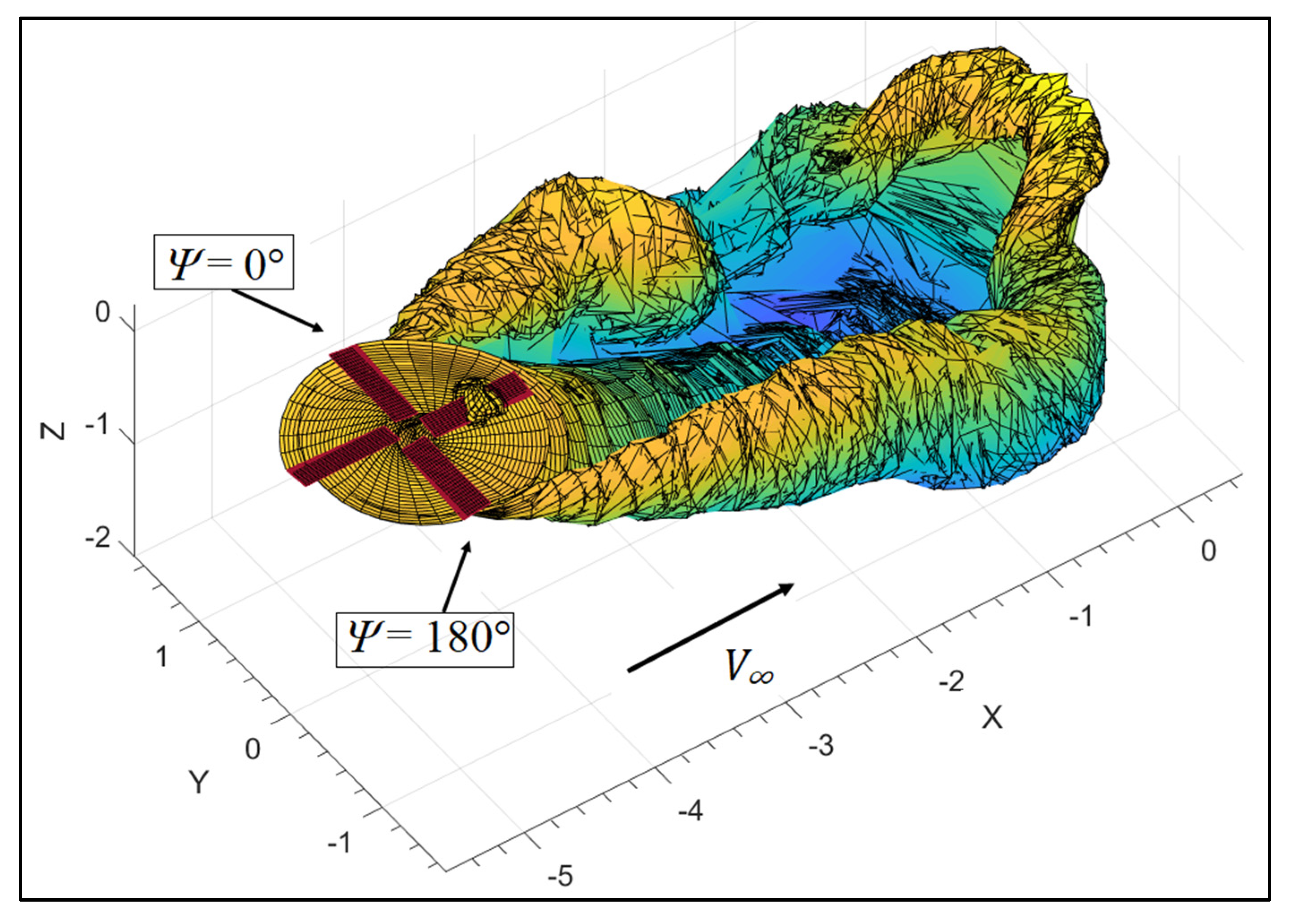
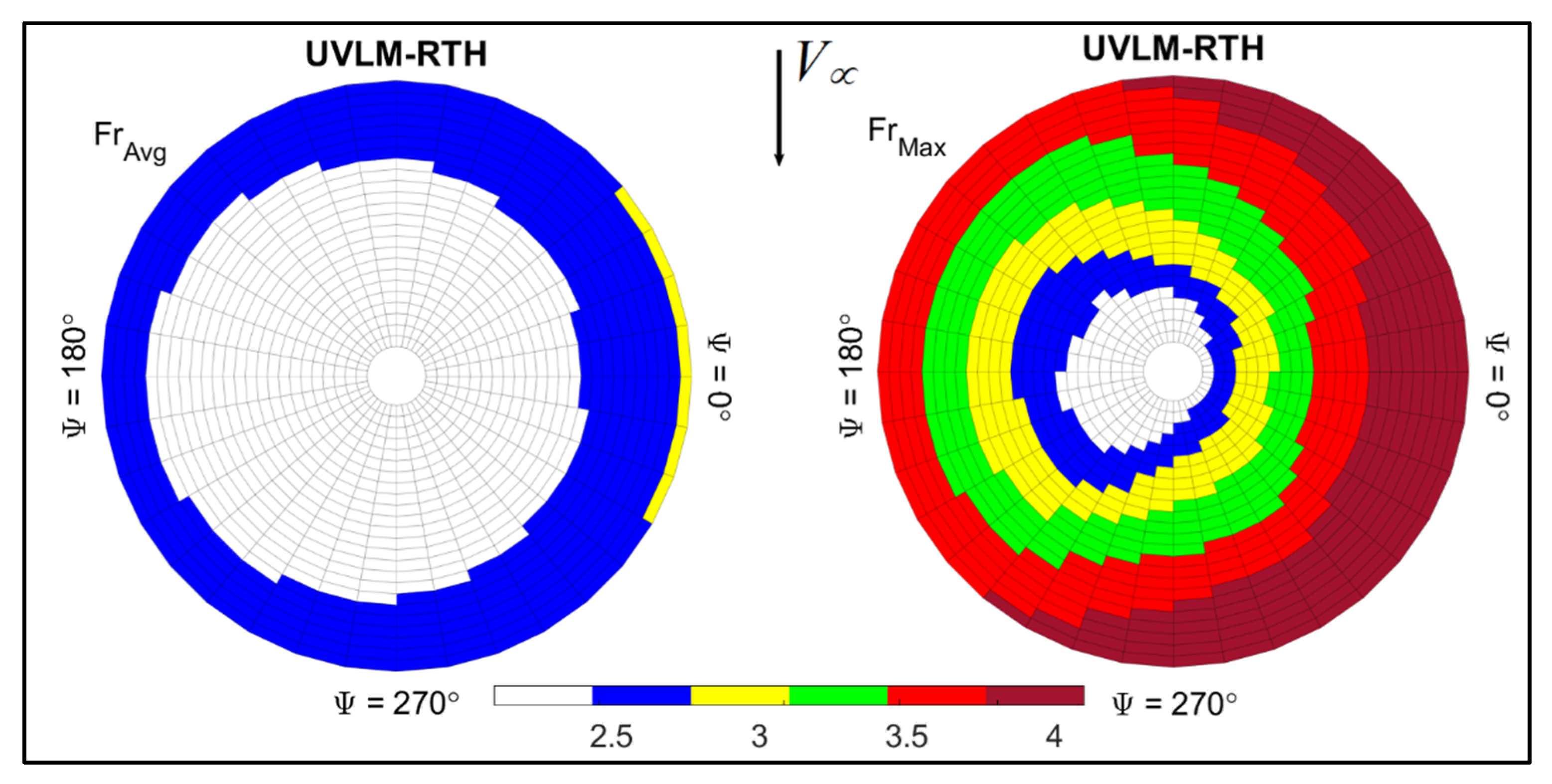
3.3.4. Forward Flight

The rotor is spinning at Ω = 2292 rpm and the advance ratio AR is 10%, this way, the maximum Re is maintained below 3 × 10⁶ for the sake of validity of Fr correlations. Blade flapping is not modeled to simplify the problem in this work. The UVLM was run using 15 × 40 vortex lattices at ΔΨ = 10° for 12 revolutions.

For a rotor in forward flight without trim and flapping blades, a dissymmetry of lift exists across the rotor disk due to the presence of advancing and retreating blade regions. More specifically, the local velocity across the blade length is not only a function of the radius due to rotation but also depends on the blade azimuth as described in Equation (25).

$$\mathrm{Re}=f(r,\mathsf{\Psi })=\left[\mathsf{\Omega }\times r+V_{\infty }\times \cos (\mathsf{\Psi })\times \cos (\theta )\right]\times \raisebox{1ex}{$\rho c$}\!\left/ \!\raisebox{-1ex}{$\mu $}\right.$$

(25)

Figure 20 shows the steady state contours of the Re and α_eff for the simulated rotor. The direction of the incoming freestream velocity due to the forward motion of the rotor is indicated by the arrow in the figure. The left side of Figure 20 shows that the retreating side of the blade, where the local blade velocity decreases, is between for 90° < Ψ < 270° and the advancing side, associated with an increase in the local blade velocity, is between 270° < Ψ < 90°. In this specific simulation, the inertial frame of reference is positioned in a way that the maximum Re is at Ψ = 0° (tip velocity is maximum), minimum is at Ψ = 180° and the tip velocity is exactly equal Ω × R_Tip at Ψ = 90° and Ψ = 270°.

The α_eff on the right side of Figure 20 was determined using the viscous coupling algorithm presented in Section 2.3.5. The highest values can be seen in the region between 280° < Ψ < 60° in the advancing blade region that moves away from the trailing wake. Considering the very low values of α_eff (≈ 0°) in the opposite Ψ region, the symmetric airfoil profile used indicates that the majority of the rotor forces will be generated in the quadrant where α_eff is maximum, representing the dissymmetry of lift. There also exists a region where α_eff is minimum and can be found between 100° < Ψ < 260° in the retreating side of the blade. This region corresponds to the reverse flow region. With these minimum α_eff, the loads generated by the blade are also at a minimum.

Figure 21 shows the wake shape produced by the simulated four-blade rotor in forward flight. The wake shown is for the complete 12 simulated revolutions that started with a stationary rotor. The direction of the incoming freestream velocity due to the forward motion of the rotor is indicated by the arrow in the figure and the positions of the Ψ of reference are indicated.

The wake shape agrees with what is expected of a four-blade rotor in forward flight, compared to the literature of similar geometries and analyses [44,47]. The roll on the edges of the wake as well as the self-induced downwash are noted, which are expected in similar flight conditions. The trailing wake behind the advancing blade is expanding more than that produced by the retreating blade, producing an asymmetric wake. This could explain the higher α_eff in the quadrant 280° < Ψ < 60°, since the denser, more expanded wake could have had a bigger influence on the α_eff, similar to what was previously seen for the IGE rotor test case.

Finally, Figure 22 shows the steady state contours of the FrAvg and FrMax for the simulated rotor in forward flight. In the left side of the figure, the predicted values of Fr_Avg vary between a minimum of 0.85 near the hub of the retreating blade side (Ψ = 180°) and a maximum of 2.8 on the tip of the advancing blade (Ψ = 0°). In general, the contour of Fr values in forward flight is shifted to the side of the retreating blade compared to the almost symmetrical Fr contours predicted for the case of the hovering rotor. The highest Fr values are seen in the region of the advancing side mainly due to the higher velocities compared to the retreating side, indicating that the Re has a stronger influence than the α_eff on the Fr_Avg.

The Fr_Max seems to be equally influenced by the α_eff as the Re. This is seen in the right side of Figure 22 where the highest values are also predicted in the advancing side of the blade but are more concentrated to the region where the α_eff values are highest in Figure 20. The Fr_Max values vary between a minimum of 1.25 near the hub of the retreating blade (Ψ = 180°) and a maximum of 4.2 on the tip of the advancing blade at Ψ = 0°, almost 30% greater than the Fr_Avg values.

4. Conclusions and Future Work

This paper presents the use of the BEMT-RHT and UVLM-RHT, two classical aerodynamic methods adapted to calculate the heat transfer on the blades of a helicopter rotor. This was achieved by linking the methods via viscous coupling to a database of RANS CFD simulations obtained using SU2. CFD simulations on a NACA 0012 allowed the calculation of the Fr_Avg and the Fr_Max on the wall of the airfoil. The data were correlated based on Re, α_eff, and Pr. The correlation was used with the BEMT and UVLM to calculate the radial heat transfer of a rotor in different flight conditions.

CFD simulations on flat plate test cases showed that the calculated Fr_x matched the one predicted by other implementations with the same turbulence model from the literature. A 7% discrepancy was also found when the Fr_x was compared to existing correlations. The implemented BEMT predicted C_T and CL_y values 15% to 20% higher than experiments for a hovering rotor, typical to the BEMT whereas the UVLM provided 98% agreement. The TVAL and TVRL by the UVLM agreed within 90% for a rotor in ground effect and axial flight, although it failed extreme ground effect. The UVLM was also validated within 75% compared to experiment results of a forward flight test case, although 87% agreement with a free wake method from the literature was noted.

A modified version of the Bell 429 tail rotor was used to quantify the steady state radial distribution of the Fr_Avg and the Fr_Max. The rotor was modeled in different flight conditions. It was found that the Fr_Avg predicted by the BEMT-RHT and the UVLM-RHT was similar with no more than 5% disagreement in values. The Fr_Max was overestimated by the BEMT-RHT by around 11% due to a higher predicted α_eff. Although both methods provided relatively quick results, the BEMT-RHT takes a fraction of the simulation time compared to the UVLM-RHT. For the test cases in hover and axial flight, the proposed Fr correlations showed that the Re has a greater impact on the heat transfer than the α_eff predicted by the BEMT or UVLM. The ground effect increased the α_eff of the hovering rotor, but no major changes were remarked in terms of Fr. Finally, for the rotor in forward flight, the Fr_Avg showed greater dependency on the Re whereas the Fr_Max was equally dependent on the α_eff and more influenced by the wake position relative to the blades.

Future work is about validating the methodologies of the BEMT-RHT and UVLM-RHT. Uncertainties are present especially since transitional flow features and oscillations due to rotation cannot be modeled using an approximate approach. Experimental work on a fixed wing and a rotor in an icing wind tunnel are the next phase of this research project. This will address the uncertainties associated with the application of these simplified numerical tools and quantify their limitations.

References

1. Guidelines for Aircraft Ground Icing Operations, 3rd ed.; Transport Canada: Ottawa, ON, Canada, 2018.
2. Helicopter Flying Handbook; Branch, A.T.S. (Ed.) United States Department of Transportation—Federal Aviation Administration: Washington, DC, USA, 2012.
3. Reid, T.; Baruzzi, G.S.; Habashi, W.G. FENSAP-ICE: Unsteady conjugate heat transfer simulation of electrothermal de-icing. J. Aircr. 2012, 49, 1101–1109. [Google Scholar] [CrossRef]
4. Pourbagian, M.; Habashi, W.G. Parametric analysis of energy requirements of in-flight ice protection systems. In Proceedings of the 20th Annual conference of the CFD society of Canada, Canmore, AB, Canada, 9–11 May 2012. [Google Scholar]
5. Hannat, R.; Morency, F. Numerical validation of conjugate heat transfer method for anti-/de-icing piccolo system. J. Aircr. 2014, 51, 104–116. [Google Scholar] [CrossRef]
6. Mu, Z.; Lin, G.; Shen, X.; Bu, X.; Zhou, Y. Numerical simulation of unsteady conjugate heat transfer of electrothermal deicing process. Int. J. Aerosp. Eng. 2018, 2018, 5362541. [Google Scholar] [CrossRef]
7. Gallay, S.; Laurendeau, E. Nonlinear generalized lifting-line coupling algorithms for pre/poststall flows. AIAA J. 2015, 53, 1784–1792. [Google Scholar] [CrossRef]
8. Van Dam, C. The aerodynamic design of multi-element high-lift systems for transport airplanes. Prog. Aerosp. Sci. 2002, 38, 101–144. [Google Scholar] [CrossRef] [Green Version]
9. Gallay, S.; Laurendeau, E. Preliminary-design aerodynamic model for complex configurations using lifting-line coupling algorithm. J. Aircr. 2016, 53, 1145–1159. [Google Scholar] [CrossRef]
10. Parenteau, M.; Plante, F.; Laurendeau, E.; Costes, M. Unsteady Coupling Algorithm for Lifting-Line Methods. In Proceedings of the 55th Aerospace Sciences Meeting, Grapevine, TX, USA, 9–13 January 2017; p. 0951. [Google Scholar]
11. Parenteau, M.; Sermeus, K.; Laurendeau, E. VLM Coupled with 2.5 D RANS Sectional Data for High-Lift Design. In Proceedings of the 55th Aerospace Sciences Meeting, Kissimmee, FL, USA, 8–12 January 2018; p. 1049. [Google Scholar]
12. Bourgault-Cote, S.; Parenteau, M.; Laurendeau, E. Quasi-3D multi-layer ice accretion model using a Vortex Lattice Method combined with 2.5 D RANS solutions. In Proceedings of the 54rd 3AF International Conference on Applied Aerodynamics, Paris, France, 25–27 March 2019. [Google Scholar]
13. Edmunds, M.; Malki, R.; Williams, A.; Masters, I.; Croft, T. Aspects of tidal stream turbine modelling in the natural environment using a coupled BEM–CFD model. Int. J. Mar. Energy 2014, 7, 20–42. [Google Scholar] [CrossRef] [Green Version]
14. Masters, I.; Malki, R.; Williams, A.J.; Croft, T.N. The influence of flow acceleration on tidal stream turbine wake dynamics: A numerical study using a coupled BEM–CFD model. Appl. Math. Model. 2013, 37, 7905–7918. [Google Scholar] [CrossRef]
15. Sun, Z.; Chen, J.; Shen, W.Z.; Zhu, W.J. Improved blade element momentum theory for wind turbine aerodynamic computations. Renew. Energy 2016, 96, 824–831. [Google Scholar] [CrossRef]
16. Olczak, A.; Stallard, T.; Feng, T.; Stansby, P. Comparison of a RANS blade element model for tidal turbine arrays with laboratory scale measurements of wake velocity and rotor thrust. J. Fluids Struct. 2016, 64, 87–106. [Google Scholar] [CrossRef]
17. Colmenares, J.D.; López, O.D.; Preidikman, S. Computational study of a transverse rotor aircraft in hover using the unsteady vortex lattice method. Math. Probl. Eng. 2015, 2015, 478457. [Google Scholar] [CrossRef] [Green Version]
18. Chung, K.H.; Kim, J.W.; Ryu, K.W.; Lee, K.T.; Lee, D.J. Sound generation and radiation from rotor tip-vortex pairing phenomenon. Am. Inst. Aeronaut. Astronaut. 2006, 44, 1181–1187. [Google Scholar] [CrossRef]
19. Ferlisi, C. Rotor Wake Modelling Using the Vortex-Lattice Method. Master’s Thesis, École Polytechnique de Montréal, Montréal, QC, Canada, 2018. [Google Scholar]
20. Pérez, A.M.; Lopez, O.; Poroseva, S.V. Free-Vortex Wake and CFD Simulation of a Small Rotor for a Quadcopter at Hover. In Proceedings of the AIAA Scitech 2019 Forum, San Diego, CA, USA, 7–11 January 2019; p. 0597. [Google Scholar]
21. Bhagwat, M.J.; Leishman, J.G. Generalized viscous vortex model for application to free-vortex wake and aeroacoustic calculations. In Proceedings of the Paper presented at the 58th Annual Forum Proceedings- American Helicopter Society, Montreal, QC, Canada, 11–13 June 2002. [Google Scholar]
22. Poinsatte, P.E. Heat Transfer Measurements from a NACA 0012 Airfoil in Flight and in the NASA Lewis Icing Research Tunnel. Master’s Thesis, University of Toledo, Toledo, OH, USA, 1990. [Google Scholar]
23. Poinsatte, P.E.; Newton, J.E.; De Witt, K.J.; Van Fossen, G.J. Heat transfer measurements from a smooth NACA 0012 airfoil. J. Aircr. 1991, 28, 892–898. [Google Scholar] [CrossRef]
24. Henry, R.C.; Guffond, D.; Garnier, F.; Bouveret, A. Heat transfer coefficient measurement on iced airfoil in small icing wind tunnel. J. Thermophys. Heat Transf. 2000, 14, 348–354. [Google Scholar] [CrossRef]
25. Wang, X.; Bibeau, E.; Naterer, G. Experimental correlation of forced convection heat transfer from a NACA airfoil. Exp. Therm. Fluid Sci. 2007, 31, 1073–1082. [Google Scholar] [CrossRef]
26. Wang, X.; Naterer, G.; Bibeau, E. Convective heat transfer from a NACA airfoil at varying angles of attack. J. Thermophys. Heat Transf. 2008, 22, 457–463. [Google Scholar] [CrossRef]
27. Li, G.; Gutmark, E.J.; Ruggeri, R.T.; Mabe, J. Heat Transfer and Pressure Measurements on a Thick Airfoil. J. Aircr. 2009, 46, 2130–2138. [Google Scholar] [CrossRef]
28. Incropera, F.P.; Lavine, A.S.; Bergman, T.L.; DeWitt, D.P. Fundamentals of Heat and Mass Transfer, 7th ed.; John Wiley & Sons: New York, NY, USA, 2007. [Google Scholar]
29. Abdollahzadeh, M.; Esmaeilpour, M.; Vizinho, R.; Younesi, A.; Pàscoa, J. Assessment of RANS turbulence models for numerical study of laminar-turbulent transition in convection heat transfer. Int. J. Heat Mass Transf. 2017, 115, 1288–1308. [Google Scholar] [CrossRef]
30. Rumsey, C.; Smith, B.; Huang, G. 2D Finite Flat Plate Validation Case. Available online: https://turbmodels.larc.nasa.gov/finiteflatplatenumerics_val.html (accessed on 1 August 2019).
31. Rumsey, C.; Smith, B.; Huang, G. 2D NACA 0012 Airfoil Validation Case. Available online: https://turbmodels.larc.nasa.gov/naca0012_val.html (accessed on 1 August 2019).
32. Kays, W.M. Convective Heat and Mass Transfer; Tata McGraw-Hill Education: New York, NY, USA, 2012. [Google Scholar]
33. Leishman, G.J. Principles of Helicopter Aerodynamics with CD Extra; Cambridge University Press: New York, NY, USA, 2006. [Google Scholar]
34. Katz, J.; Plotkin, A. Low Speed Aerodynamics, 2nd ed.; Cambridge University Press: New York, NY, USA, 2001; Volume 13. [Google Scholar]
35. Leishman, J.G.; Bhagwat, M.J.; Bagai, A. Free-vortex filament methods for the analysis of helicopter rotor wakes. J. Aircr. 2002, 39, 759–775. [Google Scholar] [CrossRef]
36. Glauert, H. The effect of compressibility on the lift of an aerofoil. Proc. R. Soc. 1928, 118, 113–119. [Google Scholar]
37. Aupoix, B.; Spalart, P. Extensions of the Spalart–Allmaras turbulence model to account for wall roughness. Int. J. Heat Fluid Flow 2003, 24, 454–462. [Google Scholar] [CrossRef]
38. Samad, A.; Morency, F.; Volat, C. A Numerical Model of the Blade Element Momentum Method for Rotating Airfoils with Heat Transfer Calculation. In Proceedings of the Joint Thermophysics and Heat Transfer Conference, Atlanta, GA, USA, 25–29 June 2018; p. 4077. [Google Scholar]
39. Caradonna, F.X.; Tung, C. Experimental and analytical studies of a model helicopter rotor in hover. In Proceedings of the 6th European Rotorcraft and Powered Lift Aircraft Forum, Bristol, UK, 16–19 September 1980. [Google Scholar]
40. Light, J.S. Tip vortex geometry of a hovering helicopter rotor in ground effect. J. Am. Helicopter Soc. 1993, 38, 34–42. [Google Scholar] [CrossRef]
41. Cheeseman, I.; Bennett, W. The Effect of Ground on a Helicopter Rotor in Forward Flight; Ministry of Supply: London, UK, 1955. [Google Scholar]
42. Caradonna, F. Performance measurement and wake characteristics of a model rotor in axial flight. J. Am. Helicopter Soc. 1999, 44, 101–108. [Google Scholar] [CrossRef]
43. Cross, J.L. Tip Aerodynamics and Acoustics Test: A Report and Data Survey; NASA Ames Research Center: Moffett Field, CA, USA, 1988. [Google Scholar]
44. Tan, J.; Wang, H. Panel/full-span free-wake coupled method for unsteady aerodynamics of helicopter rotor blade. Chin. J. Aeronaut. 2013, 26, 535–543. [Google Scholar] [CrossRef] [Green Version]
45. Kim, J.W.; Park, S.H.; Yu, Y.H. Euler and Navier-Stokes simulations of helicopter rotor blade in forward flight using an overlapped grid solver. In Proceedings of the 19th AIAA Computational Fluid Dynamics, San Antonio, TX, USA, 22–25 June 2009; p. 4268. [Google Scholar]
46. Lee, J.B.; Yee, K.J.; Oh, S.J.; Kim, D.H. Development of an unsteady aerodynamic analysis module for rotor comprehensive analysis code. Int. J. Aeronaut. Space Sci. 2009, 10, 23–33. [Google Scholar] [CrossRef] [Green Version]
47. Gennaretti, M.; Bernardini, G.; Serafini, J.; Romani, G. Rotorcraft comprehensive code assessment for blade–vortex interaction conditions. Aerosp. Sci. Technol. 2018, 80, 232–246. [Google Scholar] [CrossRef]
Figure 1. Freestream flow over a two-dimensional (2D) NACA 0012 airfoil.
Aerospace 07 00090 g001
Figure 2. Zone divisions on NACA 0012 wall.
Aerospace 07 00090 g002
Figure 3. Rotor blade with velocity and force vectors: (a) side view; (b) top view.
Aerospace 07 00090 g003
Figure 4. Vortex lattice placement on a rotating two-blade rotor.
Aerospace 07 00090 g004
Figure 5. Comparison of Fr obtained by CFD versus correlations for constant: (a) Q; (b) TS.
Aerospace 07 00090 g005
Figure 6. Average Fr variation with respect to Re and α.
Aerospace 07 00090 g006
Figure 7. Fr variation for 10 considered airfoil zones.
Aerospace 07 00090 g007
Figure 8. Prediction by UVLM and BEMT compared to the literature: (a) CT; (b) CLy.
Aerospace 07 00090 g008
Figure 9. UVLM versus experimental radial and vertical tip vortex positions for the lynx rotor.
Aerospace 07 00090 g009
Figure 10. CT predictions in ground of UVLM compared to numerical and experimental data.
Aerospace 07 00090 g010
Figure 11. UVLM versus experimental radial and vertical tip vortex positions in axial flight.
Aerospace 07 00090 g011
Figure 12. Figure of merit variation versus climb ratio.
Aerospace 07 00090 g012
Figure 13. Sectional CT variation at different radial positions for a rotor in forward flight.
Aerospace 07 00090 g013
Figure 14. View of the symmetric wake produced by the four-blade rotor in hover.
Aerospace 07 00090 g014
Figure 15. Contours of steady state FrAvg and FrMax for the hovering modified Bell 429 tail rotor obtained using BEMT-RHT and UVLM-RHT.
Aerospace 07 00090 g015
Figure 16. View of the symmetric wake produced by the four-blade rotor hovering in ground effect (IGE).
Aerospace 07 00090 g016
Figure 17. Contours of steady state FrAvg and FrMax for the hovering modified Bell 429 tail rotor in ground effect obtained using UVLM-RHT.
Aerospace 07 00090 g017
Figure 18. View of the Symmetric Wake Produced by the 4-Blade Rotor in Axial Flight.
Aerospace 07 00090 g018
Figure 19. Contours of steady state FrAvg and FrMax for the modified Bell 429 tail rotor in axial flight obtained using BEMT-RHT and UVLM-RHT.
Aerospace 07 00090 g019
Figure 20. Contours of steady state Re and αeff for the modified Bell 429 tail rotor in forward flight obtained using UVLM-RHT.
Aerospace 07 00090 g020
Figure 21. View of the asymmetric wake produced by the four-blade rotor in forward flight.
Aerospace 07 00090 g021
Figure 22. Contours of steady state FrAvg and FrMax for the modified Bell 429 tail rotor in forward flight obtained using BEMT-RHT and UVLM-RHT.
Aerospace 07 00090 g022