The Industry Internet of Things (IIoT) as a Methodology for Autonomous Diagnostics in Aerospace Structural Health Monitoring

Abstract

Structural Health Monitoring (SHM), defined as the process that involves sensing, computing, and decision making to assess the integrity of infrastructure, has been plagued by data management challenges. The Industrial Internet of Things (IIoT), a subset of Internet of Things (IoT), provides a way to decisively address SHM’s big data problem and provide a framework for autonomous processing. The key focus of IIoT is operational efficiency and cost optimization. The purpose, therefore, of the IIoT approach in this investigation is to develop a framework that connects nondestructive evaluation sensor data with real-time processing algorithms on an IoT hardware/software system to provide diagnostic capabilities for efficient data processing related to SHM. Specifically, the proposed IIoT approach is comprised of three components: the Cloud, the Fog, and the Edge. The Cloud is used to store historical data as well as to perform demanding computations such as off-line machine learning. The Fog is the hardware that performs real-time diagnostics using information received both from sensing and the Cloud. The Edge is the bottom level hardware that records data at the sensor level. In this investigation, an application of this approach to evaluate the state of health of an aerospace grade composite material at laboratory conditions is presented. The key link that limits human intervention in data processing is the implemented database management approach which is the particular focus of this manuscript. Specifically, a NoSQL database is implemented to provide live data transfer from the Edge to both the Fog and Cloud. Through this database, the algorithms used are capable to execute filtering by classification at the Fog level, as live data is recorded. The processed data is automatically sent to the Cloud for further operations such as visualization. The system integration with three layers provides an opportunity to create a paradigm for intelligent real-time data quality management.

1. Introduction

The aviation industry has grown rapidly since commercial aviation started about a hundred years ago. In fact, there is a fast growth in the number of passengers, routes, and frequencies, creating an industry with high revenues and low margins, which makes it one of the most challenging businesses in the world [1]. A significant portion of aerospace operating costs is related to maintenance. Specifically, aircraft flight maintenance includes checks based on periodic inspections. In this context, routine inspections include Check A which is required after 400–600 flights hours and is performed at about 50–70 man-hours [2]. In addition, Check B is performed after 6–8 months and requires about 160–180 man-hours [3]. These checks are imperative to evaluate the health of the aircraft and assure passenger safety, while predictive maintenance could limit operational interruptions and remove the need for checks governed by a set of schedules [4].

In this context, a number of on-board sensing cases for damage detection have been proposed, in the Internet of Things (IoT) framework [5]. Specifically, a platform that uses a Pro-Trinket microcontroller, an NRF transceiver module, a Wi-Fi module, a Raspberry Pi, and two piezoelectric sensors was reported. In this architecture, a mathematical model is used to assess whether damage exists and seeks to identify its location [5]. Data is then transferred from the Raspberry Pi to the Cloud. The same authors proposed a similar IoT application in which the model was evaluated by a commercial finite element analysis software to simulate different scenarios for damage location and width [6]. In this context, an overview of technologies that support IoT applications in Structural Health Monitoring (SHM) was provided in [7]. For example, an IoT model for SHM to evaluate wine casks was proposed in [8], while an IoT application for SHM of civil infrastructures was reported in [9] and for building SHM in [10].

The Internet of Things (IoT) is regarded as the third Internet wave and is expected to provide significant benefits to both commercial and personal uses. According to Gartner, over 26 billion devices will be connected through the IoT and result in $1.9 trillion in global economic value added through sales by 2020. The IoT framework is poised to revolutionize daily living standards by enabling smarter insights from sensor technology. Everyday items from furniture, appliances, and vehicles to large structures such as buildings, bridges, and aircraft can now serve as a data hub. The streaming data provides operational and network intelligence for real-time analytics to improve the customer experience. This interconnection between sensors and communication technology creates a flexible architecture that allows objects and devices to communicate with one another to reach common goals [11]. Furthermore, the multidisciplinary nature of IoT opens the gate to new research in computing, business, engineering, and health care [12].

A typical IoT system architecture is divided into four layers including the perception, network layer, data processing, and application layers. The perception layer aims to acquire, collect, and process the data from the physical world. This can be done through temperature sensors, QR code labels, cameras, GPS terminal sensing equipment, etc. [13]. Such recorded data is then transmitted to the processing layer typically through a wireless network. It is in general challenging to connect the Wireless Sensor Network (WSN), mobile communication networks, or the Internet with each other because of the lack of uniform standardization in communication protocols. Furthermore, the data from the WSN cannot be transmitted long distance with the current limitations in transmission protocols [14]. In this context, low power wireless communication techniques such as ZigBee, 6LowPAN, LoRaWAN, and low power Wi-Fi prove to be an effective transmission for IoT network sensors within the network layer [15].

Within the data processing layer, big data processing software and storage provide a variety of solutions for the IoT. Commercial and public datacenters such as Amazon Web Services and Microsoft Azure provide computing, storage, and software resources as Cloud services, which are enabled by virtualized software stacks [16]. On the other hand, private datacenters offer basic infrastructure services by combining available software tools and services such as Torque and Oscar, as well as file storage systems such as Storage Area Network/Network Attached Storage (SAN/NAS) [16]. These data storage providers vary in how they store, index, and execute queries. Specifically, there are relational databases that allow the user to link information from different tables or different types of data buckets, while non-relational databases store data without explicit and structured mechanisms to link data from different buckets [17]. The latter are often referred to as NoSQL databases and are composed of four forms: document-based, graph-based, column-oriented, and key-value store [18]. The role of the application layer is to provide further insights based on the data transmitted [13].

The objective of this investigation is to present the development of an IoT system that can provide real-time diagnostics in SHM applications related to the aerospace industry. In this paper, the authors are proposing a framework for real-time processing of sensor data via an IoT framework. This framework can be applied to various use cases (e.g., damage detection); however, the purpose of the paper is to provide a general methodology for real-time processing of sensor data. To achieve this goal the approach presented in this manuscript is based on (i) using sensing data including such obtained by mechanical testing and nondestructive evaluation, (ii) leveraging an IoT approach to enable real-time usage of such datasets, and (iii) developing a data-preprocessing method to create diagnostics information which could be visualized both at the Fog and Cloud layers combined with user interfaces appropriate for SHM applications.

2. Methods

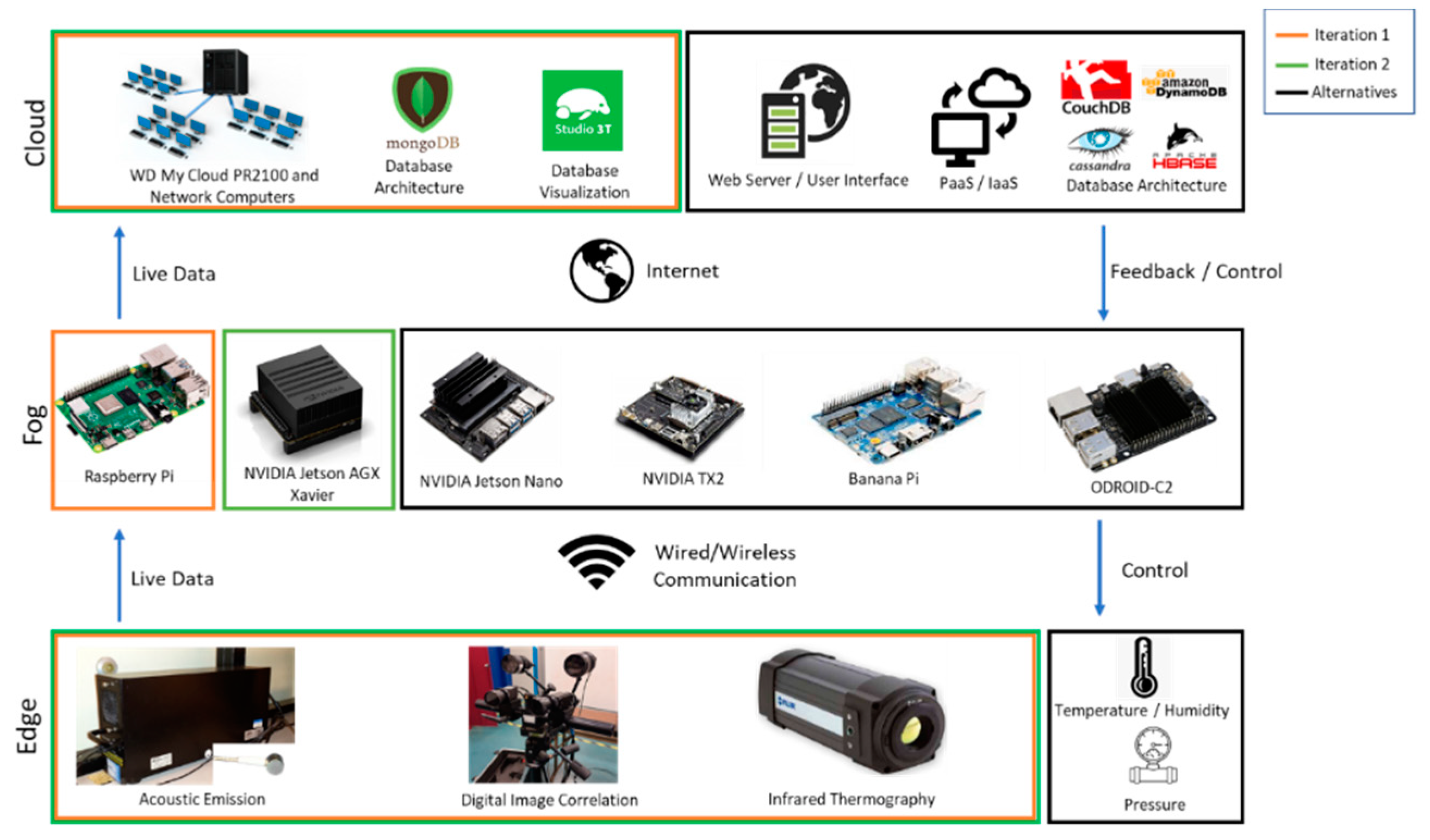
2.1. IoT Hardware & Software

The developed Industrial Internet of Things (IIoT) architecture (Figure 1) is subdivided into two parts: an onsite and a Cloud network. The system is divided into three layers namely, the Edge, Fog, and Cloud to limit the information sent to the Cloud and in order to maintain a real-time flow. The onsite network hosts the Edge and Fog layers. The Edge consists of the low-level hardware (sensors and Data Acquisition Systems (DAQs)) intended to record data from the structure being monitored. For the purposes of this investigation, the sensors are related to Non-Destructive Tensing (NDT) techniques, including Acoustic Emission (AE), Digital Image Correlation (DIC) and Infrared Thermography (IR). Other sensors (e.g., temperature, humidity, pressure) can be readily used with the proposed architecture to augment the sensing inputs. In this investigation only AE data are used to demonstrate the capabilities of the IIoT system for clarity as well as conciseness reasons.

The goal of the Fog layer is to reduce the live data stream to its most useful partitions. For the proposed IIoT architecture, the Fog layer is composed of a decentralized computing device and is tasked with aggregating, parsing, filtering, clustering, and classifying data from multiple Edge DAQs. Two design configurations were attempted to assess technical IoT characteristics related to latency, throughput, and computational efficiency. The first design iteration consisted of three Raspberry Pi 3 model B+ computers powered by ARM Cortex-A53 1.4GHz processors to compose a Raspberry Pi cluster. The purpose of the Raspberry Pi cluster is to create a concurrent pipeline which serves to subdivide tasks such as parsing the data, aggregating the data, and running the data through machine learning models into separate procedures. The procedures can be run in parallel thereby increasing the throughput of our architecture. One Raspberry Pi is used to filter incoming *.txt files from the Edge layer and store only identified features of the incoming data. Another Raspberry Pi is used to conduct a preliminary analysis on the filtered data and visualize it for local users. The third Raspberry Pi is used to concurrently run a Data Loader script to upstream data into the Cloud MongoDB database. A specified folder from the second Raspberry Pi is mapped onto each of the Edge nodes, as well as on the other two Raspberry Pis. This allows *.txt files from the Edge layer to be deposited directly into the second Raspberry Pi with limited lag.

On the second Raspberry Pi the *.txt files are then run through a filtering algorithm to only retain the useful data features. This filtered data is then directly accessible from the other two Raspberry Pis which run Python scripts to handle the data stored. The first Raspberry Pi uses this data to provide a real-time preliminary analysis to show the current signals coming into the system. The second works concurrently to ship the flittered data into the Cloud. When the test has been completed all the analysis done at the Fog level is also transferred into the Cloud.

In the second design iteration, the NVIDIA Jetson Xavier was used to optimize the data streaming processes, taking advantage of its greater computational power and faster memory read/write speeds compared to the Raspberry Pi. Other peripherals to the Jetson include one 512 GB Samsung 970 PRO SSD, one Ac 8265 Intel Dual Band Wireless chip (For WIFI and Bluetooth), one Sierra Wireless MC7455 4G LTE Transceiver Module, and accompanying connectors/antennas. Similar scripts are run on the NVIDIA Jetson to parse, filter, and visualize the data. This Fog device further has the ability to retrieve commands from the Cloud to change acquisition parameters, start and stop acquisitions, and alter algorithms running on the Fog device. Alternative single board computers are shown in Figure 1 within the system architecture. The NVIDIA Jetson Nano, NVIDIA TX2, Banana Pi, and ODROID-C2 are alternatives to a Raspberry Pi and may be used depending on the application and computational needs.

The Cloud network consists of a WD My Cloud PR2100 NAS server and two other computers. The WD My Cloud runs on a GNU/LINUX operating system and hosts a MongoDB server. MongoDB is a NoSQL database that uses a JSON document style schema to store data. The schema is flexible and provides a useful data structure for sensor data. The incoming data from the onsite network is stored in MongoDB collections on the server. This data can then be accessed by the network computers to perform further analysis. This analysis takes advantage of both the live data coming in from the Fog layer and the historical data already stored in the Cloud. The results of the analysis done at the Fog layer can be displayed to a local end user as well as uploaded back to the MongoDB server, thereby making the analysis results accessible from anywhere over an internet connection. In the implementation shown in this investigation, the link between the Cloud layer and the Fog device is achieved using Ethernet. Both TLS (Transport Layer Security) and SSL (Secure Sockets Layer) encryption are used by MongoDB in this link to enable cybersecurity measures. Feedback from the Cloud to the Fog layer enables smart feature selection, which allows for even faster cloud throughput rates. Studio 3T is used to visualize the data stored in the Cloud. Alternatives for the Cloud configuration explained can be seen in Figure 1. A webserver can be used to create a client web interface. A Platform as a Service (PaaS) or Infrastructure as a Service (IaaS) can be used to replace on-site hardware. Database architecture can vary based on the sensor data structure as well. Other NoSQL database types can be used depending on the type of sensor data. For example, a document-store database such as CouchDB, a columnar-store database such as Amazon DynamoDB, a key-value store database such as Cassandra, or Apache HBASE can be leveraged.

2.2. Data Structure

As the data is transferred through the IIoT system, data is processed to optimize computational efficiency. Starting at the Edge, raw AE waveforms (Figure 2) are recorded in the form of voltage vs. time signals from which features are extracted in a *.txt format. At the Fog layer, a low-level filtration is performed, and the resulting dataset is then uploaded to the Cloud MongoDB server. At the Fog layer, the *.txt file is converted to the binary file format Feather, to store data frames. Feather is a fast, lightweight file format created by Apache Arrow. It is language (e.g., R, Python) agnostic and has a high read and write speed. The Feather data frame is parsed and structured to a BSON format. MongoDB saves the data in the BSON file format, which is a binary encoding of JSON-type documents that MongoDB uses when storing documents as collections. Once the data is at the Cloud, onsite computers can then query the data, and the queried data is outputted in the form of data frames. Figure 2 provides an overview of the transformation of data throughout the system which constitutes the backbone of the overall IIoT approach presented in this article.

2.3. Test Case

A carbon fiber reinforced polymer composite (Hexply IM7/8552) was used in this investigation, which consisted of a 16-ply layup of 8552 epoxy resin reinforced with unidirectional IM7 carbon fiber prepreg sheets, both manufactured by Hexcel. The layup used had a [45/0/-45/90]2s stacking sequence (Figure 3). Tensile tests using a straight edge geometry cut along the orientation shown in Figure 3b were conducted based on ASTM 3039 [19,20,21]. All specimens had a final nominal thickness of 5 mm, a width of 25 mm, and a length of 250 mm in the loading direction. All specimens were loaded until failure using an MTS 370.10 Landmark servo-hydraulic load frame equipped with a 100 kN load cell. For monotonic testing, load was applied in displacement control at a rate of 2 mm/min based on ASTM 3039, while the specimens were monitored using a combination of Acoustic Emission (AE), Digital Image Correlation (DIC), and Passive Infrared Thermography (pIRT). Although this controlled tensile testing is only an idealization of actual aerospace SHM conditions, it does serve the need of a reliable and repeatable data source, which was needed to parametrize the properties and assess the performance of the proposed IIoT system.

Acoustic energy was monitored using 2 PICO sensors (150 to 750 Hz operating frequency) symmetrically placed around the center of the specimen. The first set of sensors were mounted at a distance of 25 mm from center, and the second set was mounted 75 mm from the center of the specimen. All AE waveforms were recorded at 10 Million Samples Per Second (MSPS) to avoid aliasing of the recorder waveform using a PCI-2 data acquisition board with an analog filter between 100 and 1000 kHz, which represents the closest built in filter available to the AE sensor range. Values for AE acquisition of hit were identified based on a standard Pencil Lead Break Test (PLBT) [22]. Peak Definition (PDT) was set to 100 μs, Hit Definition (HDT) was set as 500 μs, and Hit Lockout Time (HLT) was set as 500 μs. All AE equipment was manufactured by Mistras Group.

3. Results

3.1. Data Processing

The main objective of the IIoT system in this investigation is to demonstrate its capabilities to apply a data mining process to handle real-time acoustic emission data, as an example of datasets related to aerospace SHM and apply diagnostics to remove noise using machine learning methods. Previous work also by the authors verified the use of this data mining methodology for the identification of damage and noise classes in datasets obtained during fatigue testing [23,24]. In this data mining approach, features of AE data are selected using a down-selection method based on feature correlation used to eliminate highly correlated features accompanied by a Principal Component Analysis (PCA) [25,26]. Once the number of principal components is identified, an unsupervised learning approach is used to cluster data. In this investigation, a Gaussian Mixture Model (GMM) was used iteratively to compute the optimal clustering. The labels and historical data were then used to train a Support Vector Machine (SVM) model and use it for real-time data classification by uploading it to the Fog.

To demonstrate this data mining approach, Figure 4 shows actual acoustic emission datasets recorded using AE sensors, which are visualized using two of the more than twenty features that could be used to describe the voltage vs. time waveforms that are recorded in AEs, as shown in Figure 2. More specifically, Figure 4a–d portray such raw AE signals with two selected features (amplitude and peak frequency) plotted for two different datasets, one of which was used for training and the other for testing in the classification approach described in this section.

Features extracted from the datasets shown in Figure 4 were first normalized and then compared using a Pearson coefficient correlation matrix, as shown in Figure 5. Out of the initial twenty features, eighteen features were kept after the feature selection process was applied and by removing features with greater than 90% correlation.

The next step is to perform feature reduction, which decreases the feature space by choosing the optimum number of Principal Components (PCs) based on finding a point where the residuals of the next principal component do not provide additional information to the principal component space. A user-defined threshold of 95% variance was used to determine the number of PCs to describe the reduced feature space. The cut-off point for the training data is exhibited in Figure 6. As shown, the 7th PC does not significantly vary in the principal component space and is eliminated along with every component after it, giving a reduced feature space of six components.

These principal components are then used in the GMM, which was performed iteratively using 600 iterations testing the classification results achieved by attempting to group data in one up to six clusters. To mathematically determine the appropriate number of clusters, three different criteria were used and the results are shown in Figure 7. The clusters are then evaluated using the original feature space to relate classifications to specific AE data trends, which in this case are related to damage initiation and progression in the composite specimens used. The comparative criteria used include the Silhouette Coefficient, Davies-Bouldin, and Calinski Harabasz and all indicated that the optimum number of classes in this case is two. Figure 8a,b portray the clustering results for both the training and testing datasets in terms of the same two features across time, as in Figure 4. It can be seen that the classification visualized in Figure 8 shows good separation between the two clusters in the amplitude vs. time plots, while the two clusters are sufficiently distinct in the peak frequency vs. time plots.

Once the GMM clusters were defined, they were used to train a Support Vector Machine (SVM) that can associate new signals in a live monitoring case with the clusters. The SVM is actually a supervised learning method, which once trained seeks to find the best possible way to separate data [27]. The benefit of using the GMM before the SVM was to provide clustering labels for each signal and thus the SVM could use those labels to create a decision boundary. For the SVM, the general idea is to produce hyperplanes that intersect between classifications so that if a new data point falls on one side of the plane, that data point is associated with a certain class while maximizing the margin around the hyperplane [27,28]. In this investigation, the SVM was trained by using the training dataset shown in Figure 4 as well as the GMM optimal clusters. In addition, the model was trained using a radial basis function, ten iterations, and with a scale gamma parameter. Five-fold cross-validation was used to validate the SVM results using the testing dataset and the average accuracy score was 92.68% (

Table 1. Classification accuracy for the support vector machine model.

	Iteration 1	Iteration 2	Iteration 3	Iteration 4	Iteration 5	Average Cross Validation Score
SVM	92.37%	92.56%	92.44%	93.37%	92.68%	92.68%

). The SVM model was run on the Fog device and 39.87% was removed due to its noise classification, shown in blue in Figure 8.

3.2. Data Structure

During the experiment, data was ingested through the Edge and sent to the Fog and Cloud layer. At the Cloud, the data structure was finalized in a BSON format per document in the MongoDB server. Each document represents one signal thus a collection is built of many documents (Figure 9). A bulk insertion method is then used to upload the rows of the Feather data frame as individual records. Multi-document transactions are used to upload multiple documents to the existing collection in MongoDB. As the type of material or conditions change, varying collections can be created. Other sensor data can also be parsed and stored as a collection in the database. This database structure will allow querying and retrieval for model training.

3.3. System Performance

Acoustic emission data was acquired at the Edge (using a Physical Acoustics PCI2 Data Acquisition System (DAQ)) and stored on a network shared folder in the IoT device/ Raspberry Pi cluster. As per our data acquisition settings, two new data files, namely DTA (Physical Acoustics proprietary file) and *.txt, are created every second. Incoming data is appended to the files for the duration of each second until a new batch of files are created.

3.3.1. Edge to Fog Data Throughput

Using the PCI2, we recorded a throughput of 7.2 MB/s. A stopwatch was used to measure the time taken for live acoustic emission data to transfer from the Edge to the Fog. The stopwatch was concurrently started and stopped with the data acquisition procedure. This test was run three different times. Each time, the throughput was calculated by dividing the total size of the produced data (total.DTA file size) by the amount of time taken. The different throughput values were then averaged.

3.3.2. Fog to Cloud Data Throughput (Raspberry Pi Cluster)

Using the Raspberry Pi cluster, an overall average throughput of 13.2 MB/s was achieved (

Table 2. Raspberry Pi (Fog device) throughput results.

Size of Data (MB)	Processing Time (Seconds)	Throughput (MB/S)
1415	103.9	13.61
1415	115.6	12.24
1415	104.8	13.5
1415	112.2	12.61
1415	101.9	13.88

). For this test, all the data were already present on a shared folder in the Raspberry Pi cluster. The cluster was operating as described in Section 2.1. A timer was added to the MongoDB upload script and was used to measure the amount of time taken to process all the available data. The throughput was then derived by dividing the total size of the DTA files by the total processing time taken. This process was run five separate times, as shown in Table 2.

3.3.3. Fog to Cloud Data Throughput (Xavier Jetson)

Using the Xavier Jetson instead of the Raspberry Pis, an overall average throughput of 44.4 MB/s was achieved. For this test, all the data was already present on the Jetson device (1.53 GB of data). The IoT device ran two scripts for this implementation. One script (preprocessing) was parsing, filtering, and clustering. The other script (cloud portion) was in charge of uploading the data to the MongoDB server. The preprocessing portion produced a throughput of 68.3 MB/s, and the cloud upload portion produced a throughput of 44.4 MB/s. Timers were used in both scripts to measure the amount of time taken to process all the available data. The throughputs were then derived by dividing the total size of the data (DTA files) by the amount of time taken. Four iterations of this process were performed, and the mean value of the throughput results was computed (

Table 3. Jetson (Fog) device throughput results.

Size of Data (MB)	Preprocessing Time (Seconds)	Preprocessing Throughput (MB/S)	Cloud Upload Time (Seconds)	Cloud Upload Throughput (MB/S)
1530	24.44	62.60	35.98	42.51
1530	21.28	63.00	35.83	44.2
1530	20.73	73.78	33.41	45.58
1530	20.72	73.84	33.65	45.45

). Since the overall throughput of the system is throttled by its slowest performing piece, the final throughput was defined to be 44.4 MB/s.

4. Discussion

The investigation presented in this manuscript demonstrates the capability to stream live data through an IIoT framework for intelligent data quality management. Each layer of the system, the Edge, Fog, and Cloud, play a role in consolidating, filtering, and structuring live data. Again, this framework can be applied to a variety of use cases. The Edge layer is responsible for denoising analog signals. The Fog layer is responsible for performing diagnostics using an SVM model which is trained by using classification labels derived by the GMM. Additionally, the Cloud layer can send feedback parameters based on its data quality analysis to the Fog. The Fog can then use this information to adjust its data processing parameters, thereby creating an intelligent data quality management scheme. The architecture also supports dynamic model improvement. The results presented showcase a machine learning model, an SVM, applied to streaming data, thus enabling smart feature selection and data reduction at the Fog before data is sent to the Cloud. Furthermore, as historical data is stored in the Cloud server, it is structured for simple and flexible retrieval, thus enabling a continuous model training. The model can be further trained using High Performance Computing (HPC) at the cloud layer resulting, potentially, in improved computing time. The organized data structure is essential to reduce the computational burden on the Cloud and provide an opportunity to integrate multi-sensor data, as NoSQL databases provide hardware and data flexibility. In terms of hardware, the NoSQL databases can be partitioned across several servers, therefore providing an opportunity for horizontal scaling. Specifically, the BSON structure provides a custom key-value schema for structural data collected. It is important to note that the proposed IIoT framework can be applied for a variety of monitoring scenarios.

5. Concluding Remarks

The research presented showcases a system architecture for live sensor data to be transmitted from the environment to the Cloud with an intermediary Fog layer. The Fog layer is used for data filtering, structuring, and diagnostics of live signals. Although this architecture is presented for structural health monitoring applications, this architecture can be applied to other IoT applications such as smart cities, advanced manufacturing, and autonomous vehicles. Furthermore, alternative algorithms at the Fog like streaming algorithms, and additional quality metrics within the live framework (e.g., History PCA [29]) can be implemented.

References

1. Saltoğlu, R.; Humaira, N.; İnalhan, G. Aircraft scheduled airframe maintenance and downtime integrated cost model. Adv. Oper. Res. 2016, 2016. [Google Scholar] [CrossRef]
2. Kinnison, H.A.; Siddiqui, T. Aviation Maintenance Management; McGraw-Hill Education: New York, NY, USA, 2012. [Google Scholar]
3. Quantas. The A, C and D of Aircraft Maintenance. Available online: www.qantasnewsroom.com.au/roo-tales/the-a-c-and-d-of-aircraft-maintenance/ (accessed on 22 May 2020).
4. Kingsley-Jones, M. Airbus Sees Big Data Delivering 'Zero-AOG' Goal within 10 Years. Available online: https://www.flightglobal.com/mro/airbus-sees-big-data-delivering-zero-aog-goal-within-10-years/126446.article (accessed on 22 May 2020).
5. Abdelgawad, A.; Yelamarthi, K. Structural health monitoring: Internet of things application. In Proceedings of the 2016 IEEE 59th International Midwest Symposium on Circuits and Systems (MWSCAS), Abu Dhabi, UAE, 16–19 October 2016; pp. 1–4. [Google Scholar]
6. Abdelgawad, A.; Yelamarthi, K. Internet of things (IoT) platform for structure health monitoring. Wirel. Commun. Mob. Comput. 2017, 2017. [Google Scholar] [CrossRef]
7. Tokognon, C.A.; Gao, B.; Tian, G.Y.; Yan, Y. Structural health monitoring framework based on Internet of Things: A survey. IEEE Internet Things J. 2017, 4, 619–635. [Google Scholar] [CrossRef]
8. Cañete, E.; Chen, J.; Martín, C.; Rubio, B. Smart Winery: A Real-Time Monitoring System for Structural Health and Ullage in Fino Style Wine Casks. Sensors 2018, 18, 803. [Google Scholar] [CrossRef] [PubMed] [Green Version]
9. Jeong, S.; Law, K. An IoT Platform for Civil Infrastructure Monitoring. In Proceedings of the 2018 IEEE 42nd Annual Computer Software and Applications Conference (COMPSAC), Tokyo, Japan, 23–27 July 2018; IEEE: New York, NY, USA, 2018; pp. 746–754. [Google Scholar]
10. Wang, J.; Fu, Y.; Yang, X. An integrated system for building structural health monitoring and early warning based on an Internet of things approach. Int. J. Distrib. Sens. Netw. 2017, 13, 1550147716689101. [Google Scholar] [CrossRef] [Green Version]
11. Yan, Z.; Zhang, P.; Vasilakos, A.V. A survey on trust management for Internet of Things. J. Netw. Comput. Appl. 2014, 42, 120–134. [Google Scholar] [CrossRef]
12. Whitmore, A.; Agarwal, A.; Da Xu, L. The Internet of Things—A survey of topics and trends. Inf. Syst. Front. 2015, 17, 261–274. [Google Scholar] [CrossRef]
13. Lin, N.; Shi, W. The research on Internet of things application architecture based on web. In Proceedings of the 2014 IEEE Workshop on Advanced Research and Technology in Industry Applications (WARTIA), Ottawa, ON, Canada, 29–30 September 2014; pp. 184–187. [Google Scholar]
14. Sheng, Z.; Mahapatra, C.; Zhu, C.; Leung, V.C. Recent advances in industrial wireless sensor networks toward efficient management in IoT. IEEE Access 2015, 3, 622–637. [Google Scholar] [CrossRef]
15. Mahmoud, M.S.; Mohamad, A.A. A study of efficient power consumption wireless communication techniques/modules for internet of things (IoT) applications. Adv. Internet Things 2016, 6, 19–29. [Google Scholar] [CrossRef] [Green Version]
16. Wang, L.; Ranjan, R. Processing distributed internet of things data in clouds. IEEE Cloud Comput. 2015, 2, 76–80. [Google Scholar] [CrossRef]
17. Padhy, R.P.; Patra, M.R.; Satapathy, S.C. RDBMS to NoSQL: Reviewing some next-generation non-relational database’s. Int. J. Adv. Eng. Sci. Technol. 2011, 11, 15–30. [Google Scholar]
18. Han, J.; Haihong, E.; Le, G.; Du, J. Survey on NoSQL database. In Proceedings of the 2011 6th International Conference on Pervasive Computing and Applications, Port Elizabeth, South Africa, 25–29 October 2011; pp. 363–366. [Google Scholar]
19. ASTM Standard. D3039/D3039M-00. Standard Test Method for Tensile Properties of Polymer Matrix Composite Materials; ASTM International: West Conshohocken, PA, USA, 2000. [Google Scholar]
20. Marlett, K.; Ng, Y.; Tomblin, J. Hexcel 8552 IM7 Unidirectional Prepreg 190 gsm & 35% RC Qualification Material Property Data Report; Test Report CAM-RP-2009-015, Rev. A; National Center for Advanced Materials Performance: Wichita, KS, USA, 2011; pp. 1–238. [Google Scholar]
21. Stelzer, S.; Brunner, A.; Argüelles, A.; Murphy, N.; Pinter, G. Mode I delamination fatigue crack growth in unidirectional fiber reinforced composites: Development of a standardized test procedure. Compos. Sci. Technol. 2012, 72, 1102–1107. [Google Scholar] [CrossRef] [Green Version]
22. Ohtsu, M.; Enoki, M.; Mizutani, Y.; Shigeishi, M. Principles of the acoustic emission (AE) method and signal processing. In Practical Acoustic Emission Testing; Springer: Tokyo, Japan, 2016; pp. 5–34. [Google Scholar]
23. Wisner, B.; Kontsos, A. In situ monitoring of particle fracture in aluminium alloys. Fatigue Fract. Eng. Mater. Struct. 2018, 41, 581–596. [Google Scholar] [CrossRef]
24. Mazur, K.; Wisner, B.; Kontsos, A. Fatigue Damage Assessment Leveraging Nondestructive Evaluation Data. JOM 2018, 70, 1182–1189. [Google Scholar] [CrossRef]
25. Wold, S.; Esbensen, K.; Geladi, P. Principal component analysis. Chemom. Intell. Lab. Syst. 1987, 2, 37–52. [Google Scholar] [CrossRef]
26. Jackson, J.E. A User's Guide to Principal Components; John Wiley & Sons: New York, NY, USA, 2005; Volume 587. [Google Scholar]
27. Bishop, C.M. Pattern Recognition and Machine Learning; Springer: New York, NY, USA, 2006. [Google Scholar]
28. Steinwart, I.; Christmann, A. Support Vector Machines; Springer Science & Business Media: New York, NY, USA, 2008. [Google Scholar]
29. Yang, P.; Hsieh, C.-J.; Wang, J.-L. History PCA: A New Algorithm for Streaming PCA. arXiv 2018, arXiv:1802.05447. [Google Scholar]
Figure 1. Hardware and software architecture in the developed Industrial Internet of Things (IIoT) system.
Aerospace 07 00064 g001
Figure 2. Data Architecture in the developed IIoT system.
Aerospace 07 00064 g002
Figure 3. (a) Schematic of the IM7/8552 laminate fiber orientation stacking, (b) schematic of specimen orientation in relation to the manufactured composite sheet, and (c) straight edge specimen of IM7 8552 used for experimental testing in this investigation.
Aerospace 07 00064 g003
Figure 4. (a) Raw Acoustic Emission (AE) data visualized as amplitude vs. time for the training dataset; (b) raw AE data visualized as peak frequency vs. time for the training dataset; (c) raw AE data visualized as amplitude vs. time for the testing dataset; (d) raw AE data visualized as peak frequency vs. time for the testing dataset.
Aerospace 07 00064 g004
Figure 5. Pearson coefficient correlation matrix.
Aerospace 07 00064 g005
Figure 6. Variance per principal component.
Aerospace 07 00064 g006
Figure 7. Criteria used for cluster assessment.
Aerospace 07 00064 g007
Figure 8. (a) Clustering results across amplitude vs. time for the training set; (b) clustering results across peak frequency vs. time for the training set; (c) classification results across amplitude vs. time for the testing set; (d) classification results across peak frequency vs. time for the testing set.
Aerospace 07 00064 g008
Figure 9. Database structure used in the IIoT system.
Aerospace 07 00064 g009