Hybrid Metal/Composite Lattice Structures: Design for Additive Manufacturing

 , , and
Abstract
:1. Introduction
- reducing fuel consumption and the related contaminant emissions;
- reducing manufacturing costs related to the technologies and materials;
- reducing manufacturing time, enhancing assembly operations and facilitate maintenance of companies.
2. Description of the Proposed Routine
- Basic Settings: This modulus contains the commands used to define the graphic options, the definition of the file name, the title to be inserted at the bottom of the window for all the images, and the quality (resolution) of the images generated during the execution of the routine.
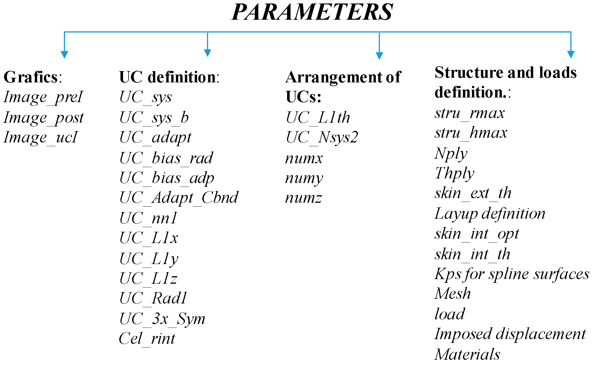
- Parameters: This modulus contains all the parameters and the options that allow to create the structure. In order to generate a consistent design, each parameter is allowed to vary in a specific range. An internal check, which enables parameters changing, was implemented to reduce the occurrence of errors. Any automatic changes are recorded on a specific output file (Calculated Parameters section). Other parameters to be defined identify the type of analysis required and the types of load and boundary conditions applied. For a quick classification, in Figure 1 the parameters are catalogued in four macro areas: graphic; unit cell definition; arrangement of unit cells; structure and loads definition.
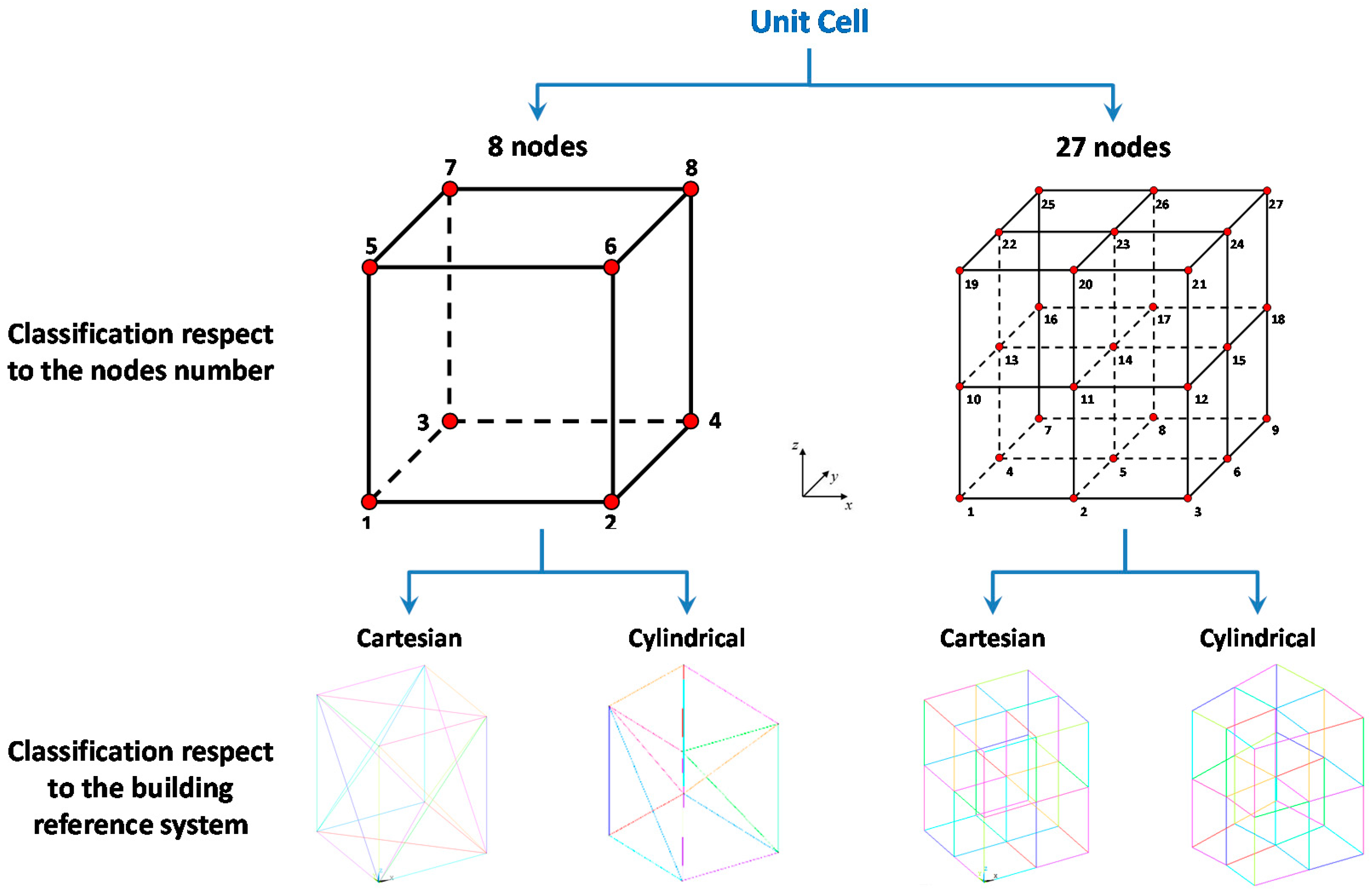
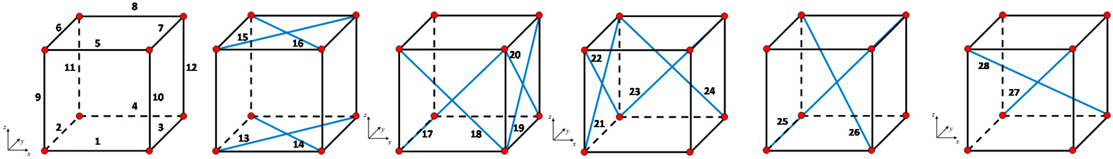
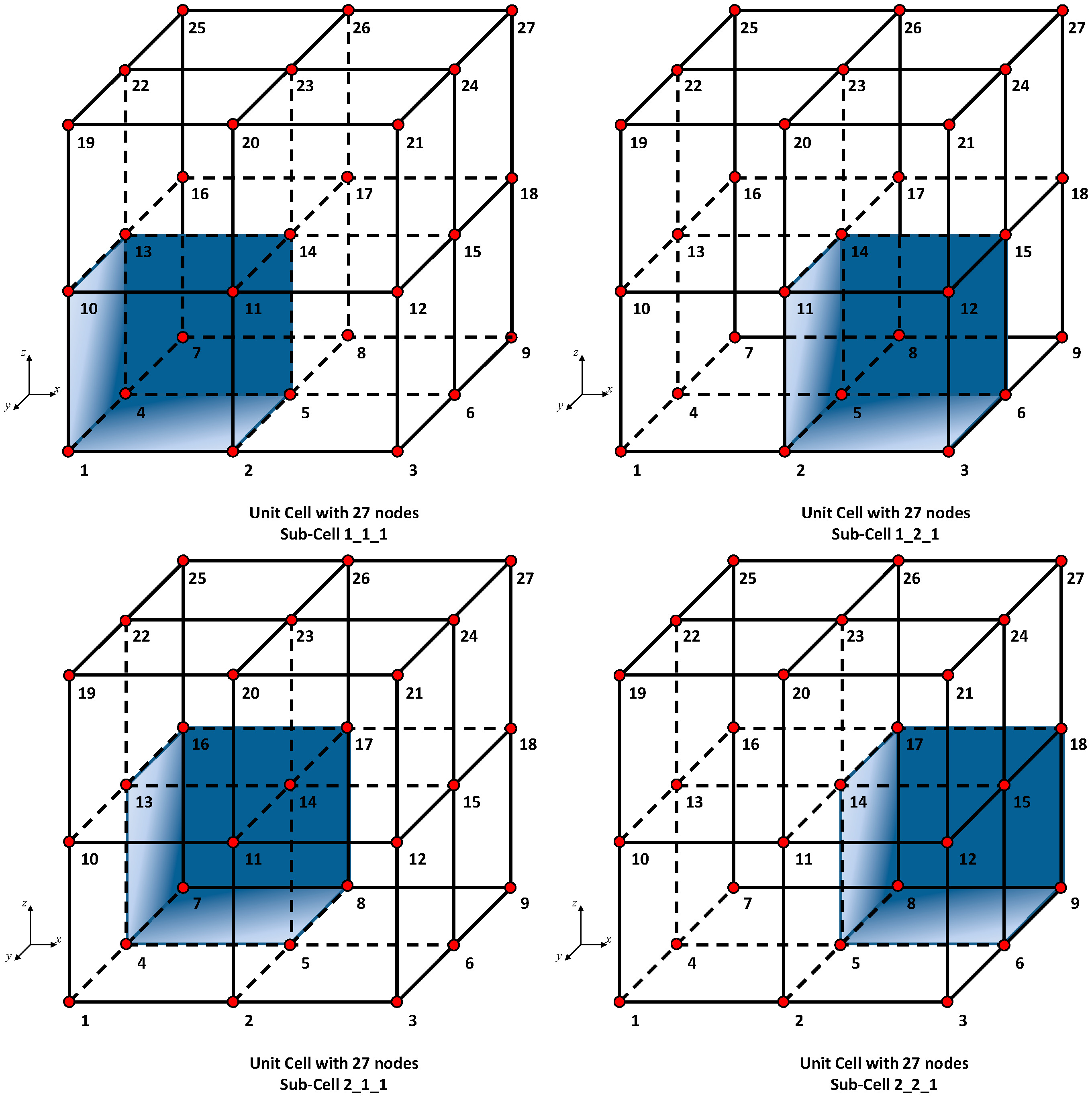
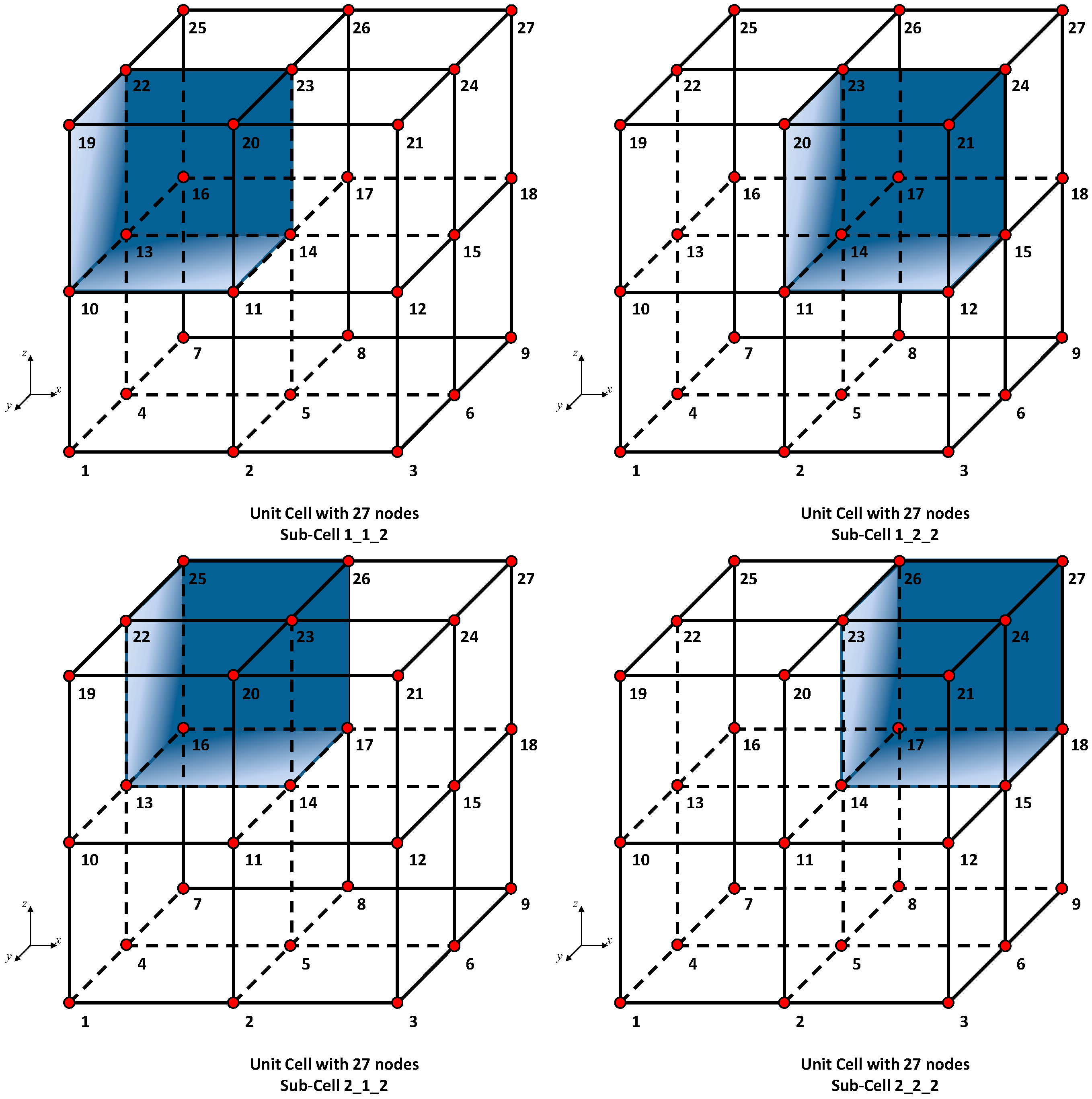
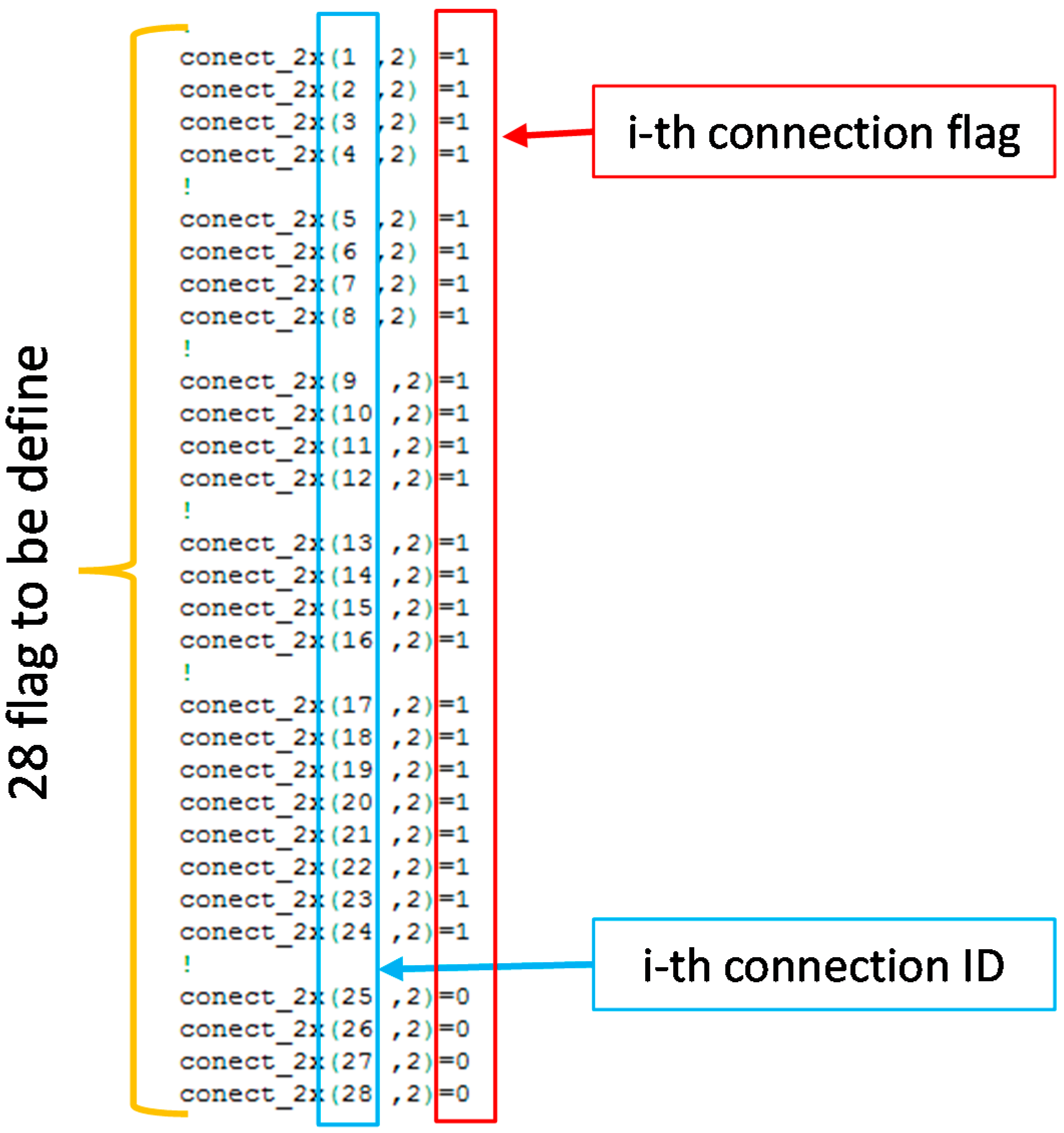
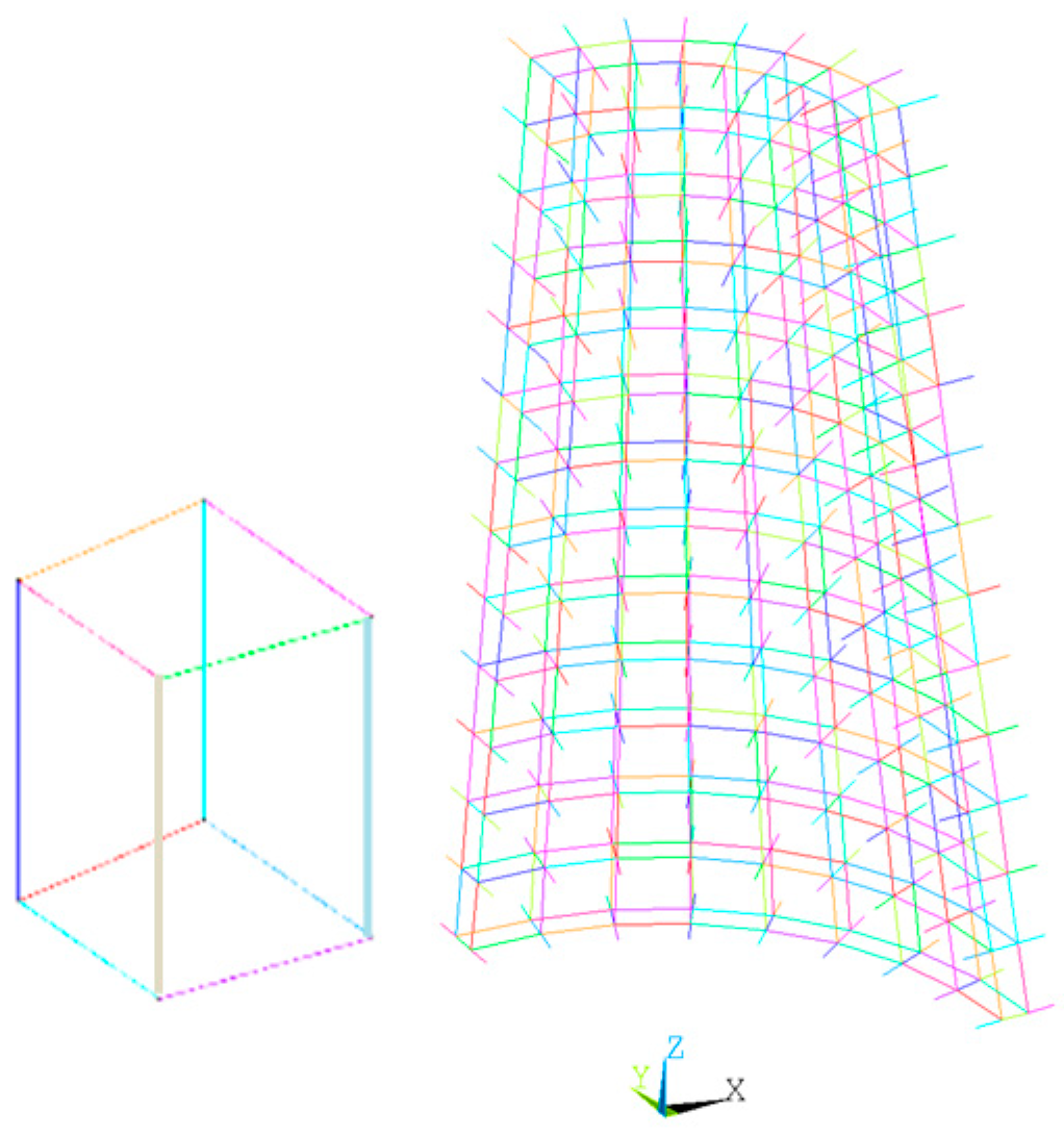
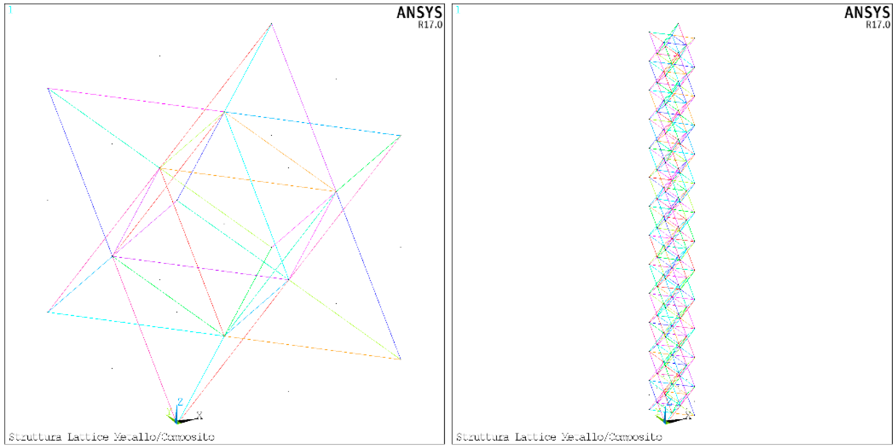
- Unit Cell Connections: In this modulus, the unit cell connections are defined. Two types of unit cell have been implemented and classified according to the number of internal nodes: 8-node and 27-node. The connection between the nodes is defined by activating a flag (1 or 0). The basic numbering for nodes and connections for both cell types are provided below. In this modulus the sequence of flags activating a predefined cell can be defined.
- Calculated Parameters: in this modulus, other parameters useful for the correct sizing of the UCs are evaluated by combining all the parameters previously defined. Moreover, parameters introduced in the previous moduli are checked and, if not consistent, they are overwritten with appropriate values. In addition, at this stage, the matrices associated to the connection flags are compiled. In this modulus, the connections are also redefined according to the symmetric option available for the 27-node unit cells.
- Elements Definition: In this modulus, the element types and the corresponding key-option, used to discretize the numerical model, are defined. Currently, four element types have been implemented:
- ○
- One-dimensional elements for the discretization of the lattice metal structure;
- ○
- Layered shell elements for the external skin;
- ○
- Shell elements for the internal skin;
- ○
- Rigid elements for the application of particular loading conditions.
- Materials and Property: This modulus specifies the material properties used for the whole model. The routine supports the modelling of the metal parts by means of linear elastic or elastoplastic, isotropic, and homogeneous material. The composite part (external skin) is modelled with a homogeneous orthotropic (or anisotropic) linear-elastic material. Since the ANSYS code requires the definition of particular sections for the attribution of mechanical and physical properties to the different parts, the sections and their options are also defined at this stage.
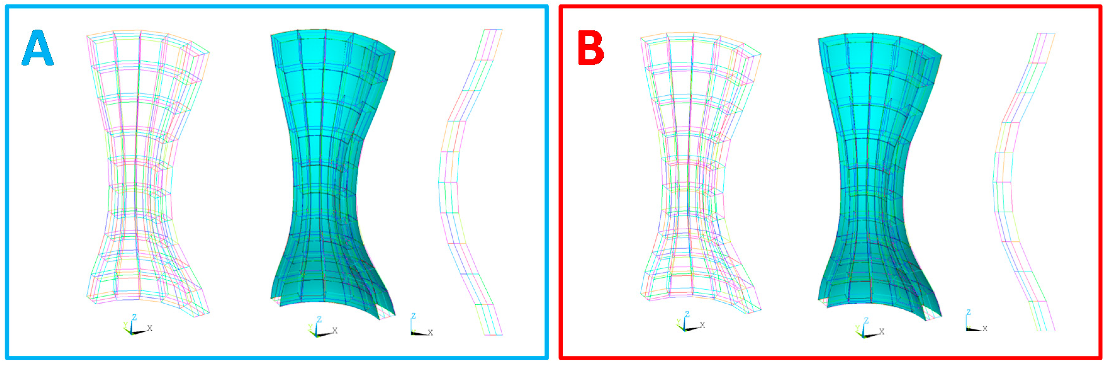
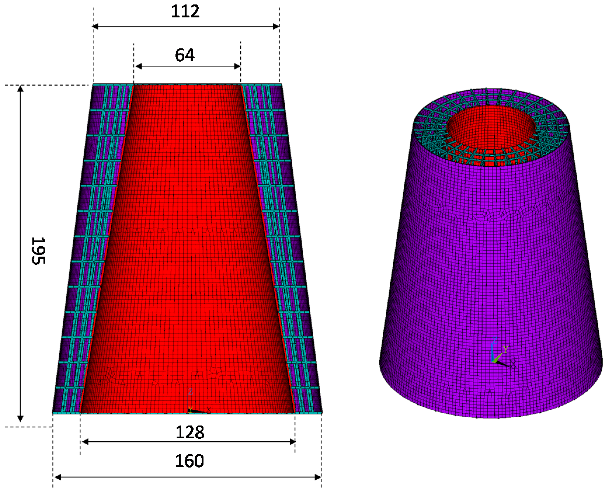
- Model Building: At this stage, the routine creates the whole geometrical model. This phase is the heart of the APDL routine. The routine is able to generate any axially symmetric hybrid structures, characterized by different shapes and sizes. Some examples are shown in Figure 2.
- Meshing: This modulus is dedicated to the mesh generation. Therefore, all the previously created geometries are discretized, according to the specification of the mesh parameters defined in the parameters section.
- Statistics: In this modulus, statistics on the model are performed. In particular, the weight of the whole structure and of each separate part (metal and/or composite), the number of both elements and nodes (of the whole model and of each separate part) are evaluated.
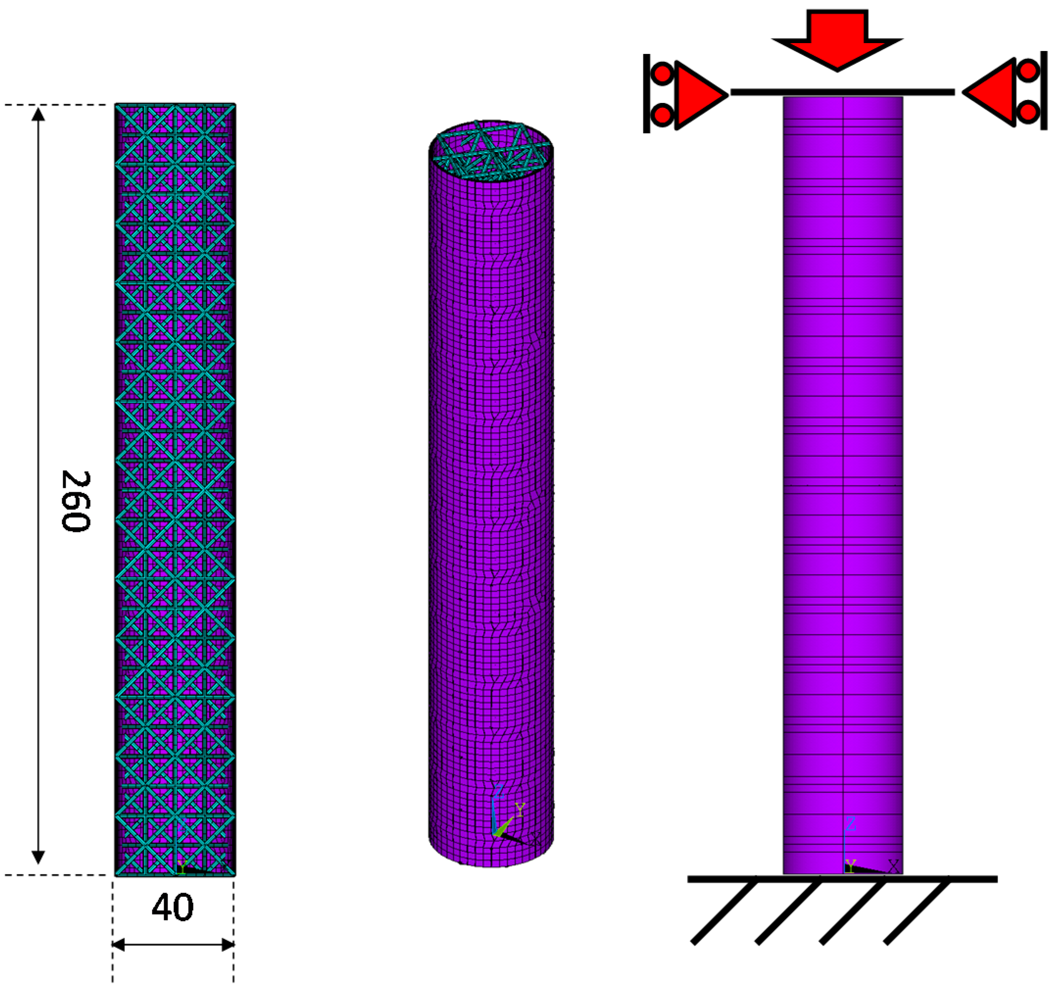
- Boundary Conditions: In this modulus, the desired loading and boundary conditions are applied to the models. Different loading types can be defined, such as compression, traction, bending, torsion, and internal and/or external pressure on both external or internal surfaces.
- Solution: This modulus defines the different types of analysis that can be performed: linear structural analysis, non-linear static analysis (non-linear buckling), and linear buckling analysis.
- Post-Processing: This modulus is dedicated to the evaluation of the optimization parameters (constraint and objective functions). These parameters are written in an output file, which can be used as input in the ModeFrontier routine. Finally, this modulus includes a specific subroutine used to generate post-processing images.
3. Unit Cell Definition
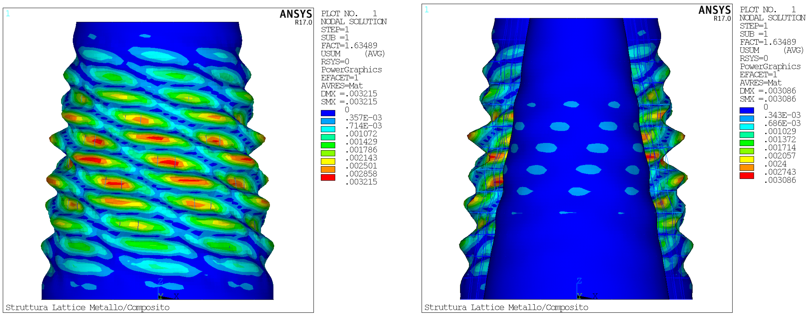
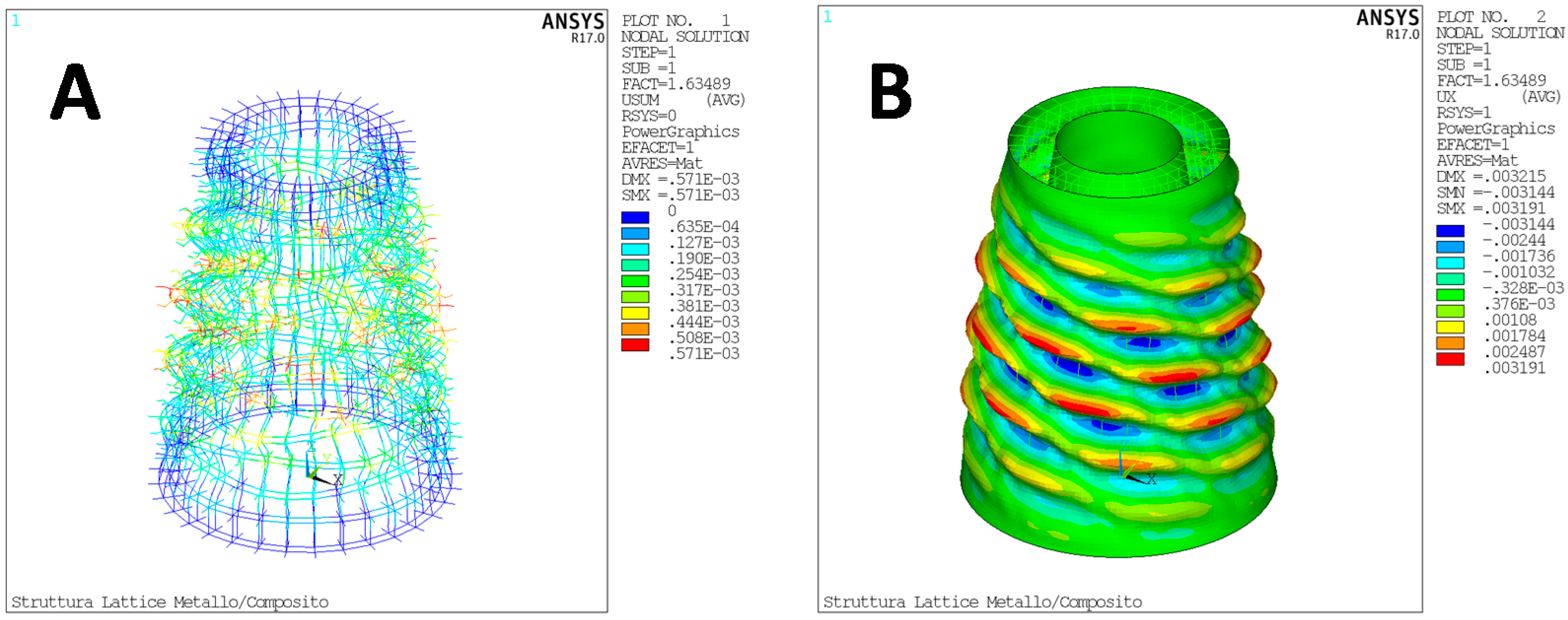
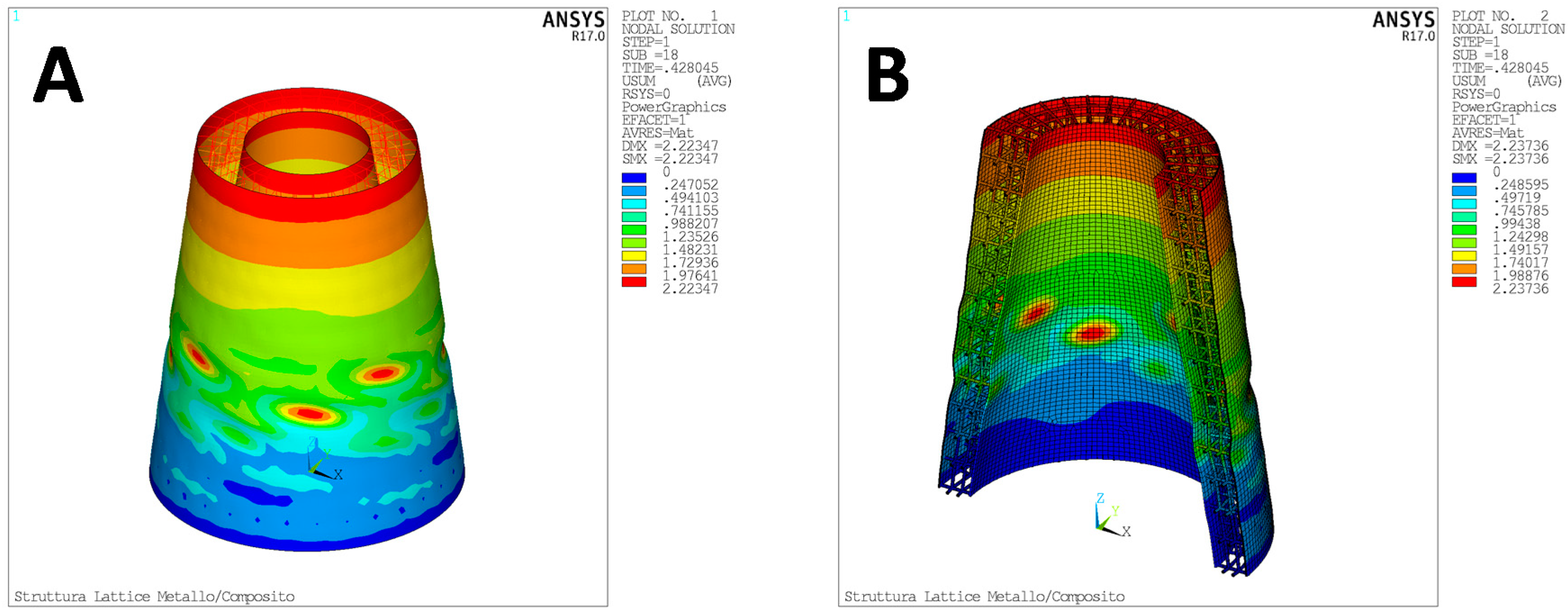
4. Numerical Results
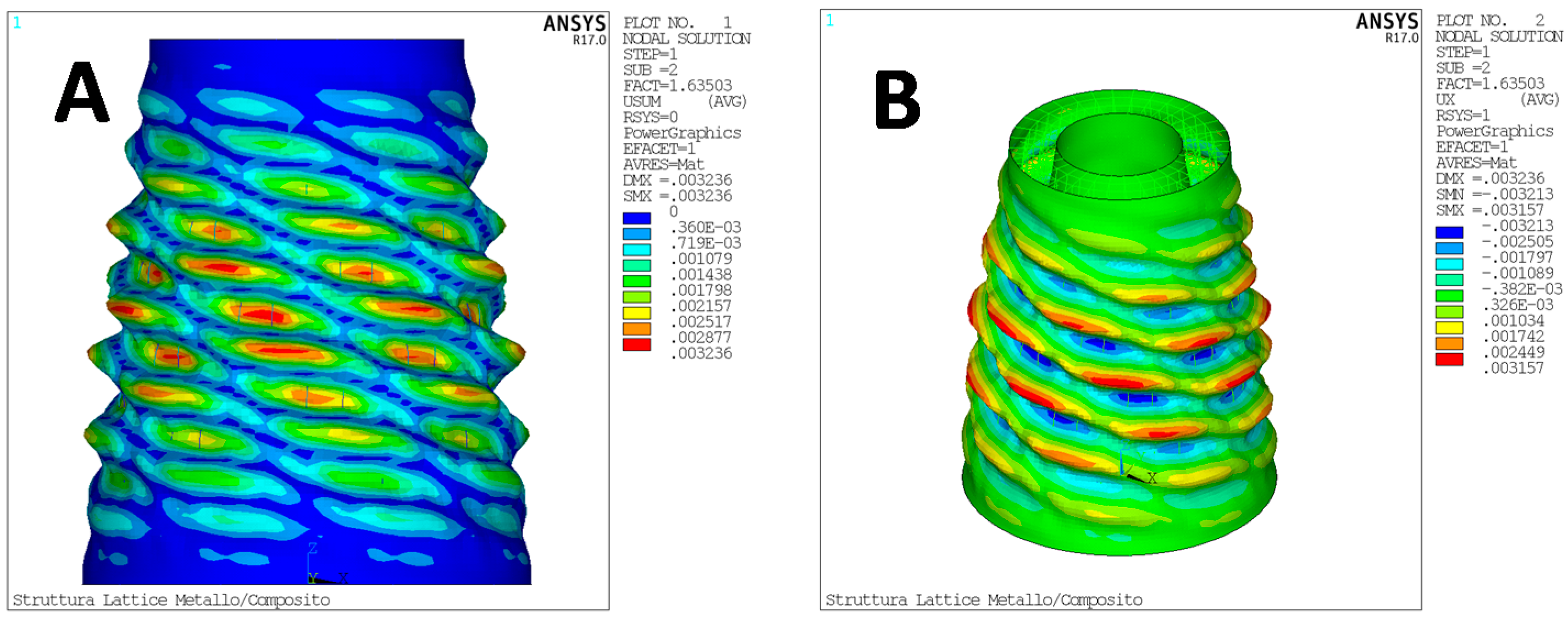
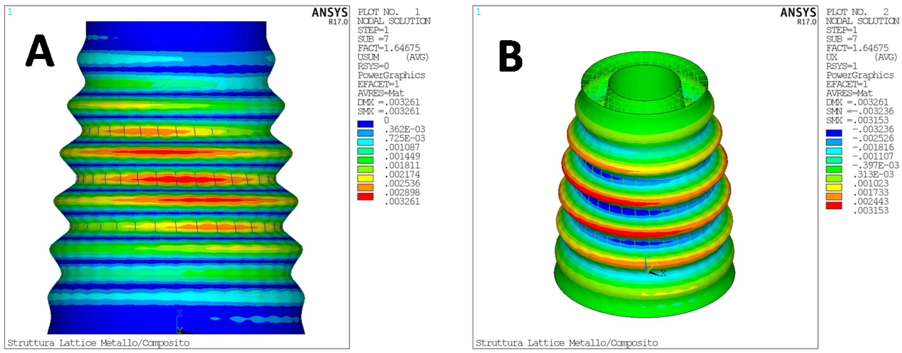
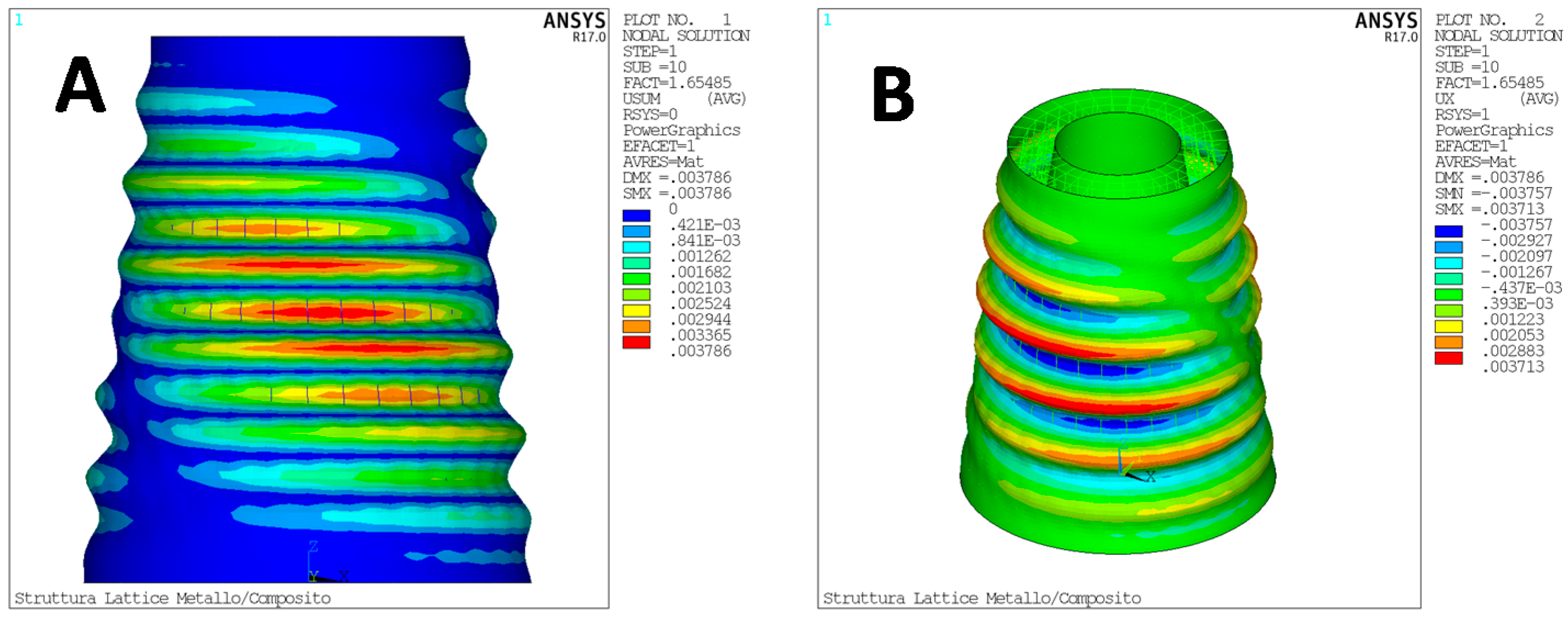
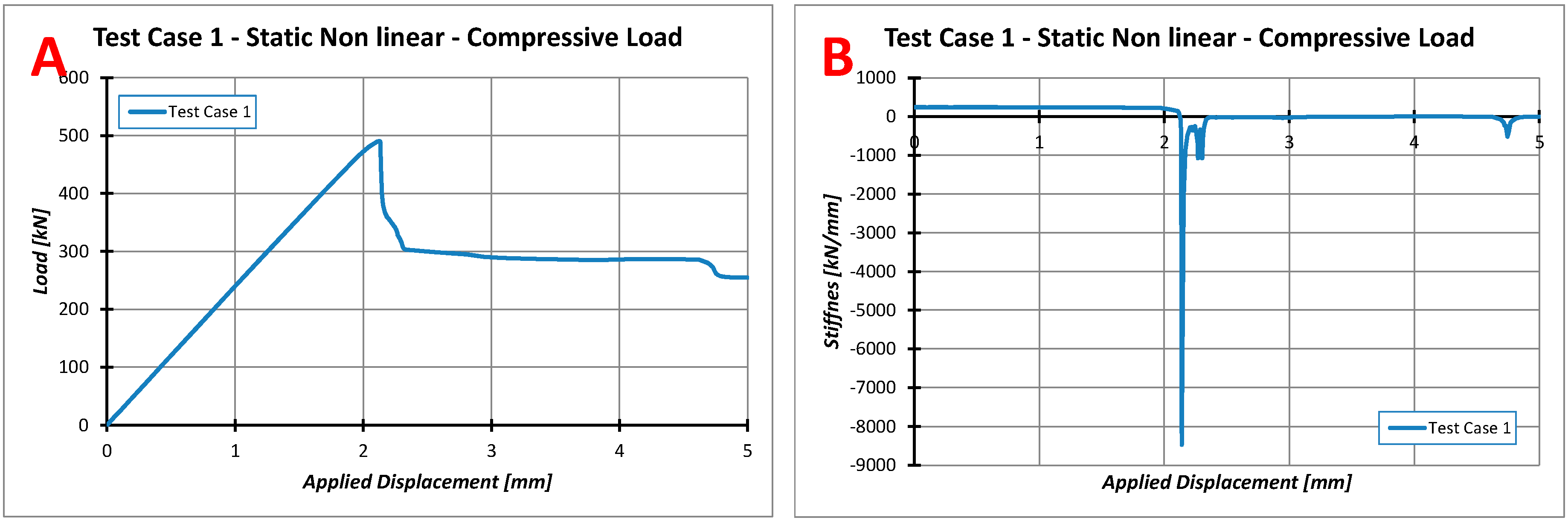
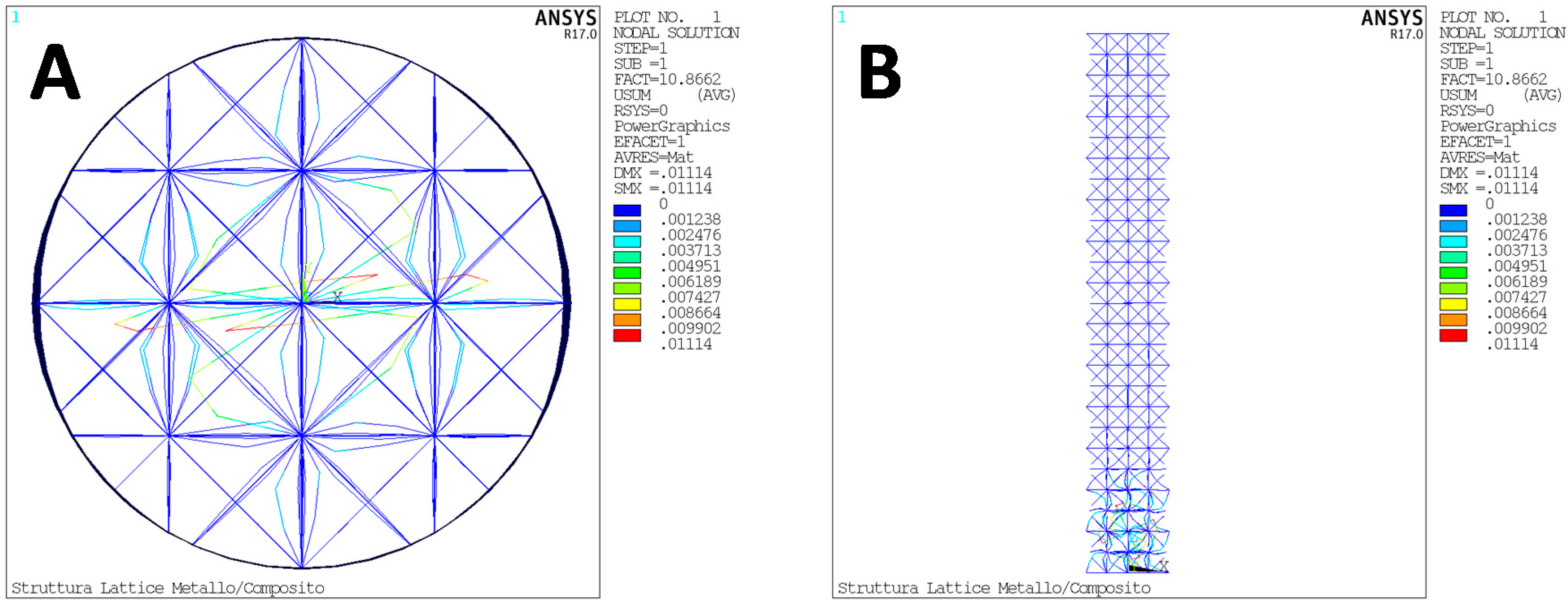
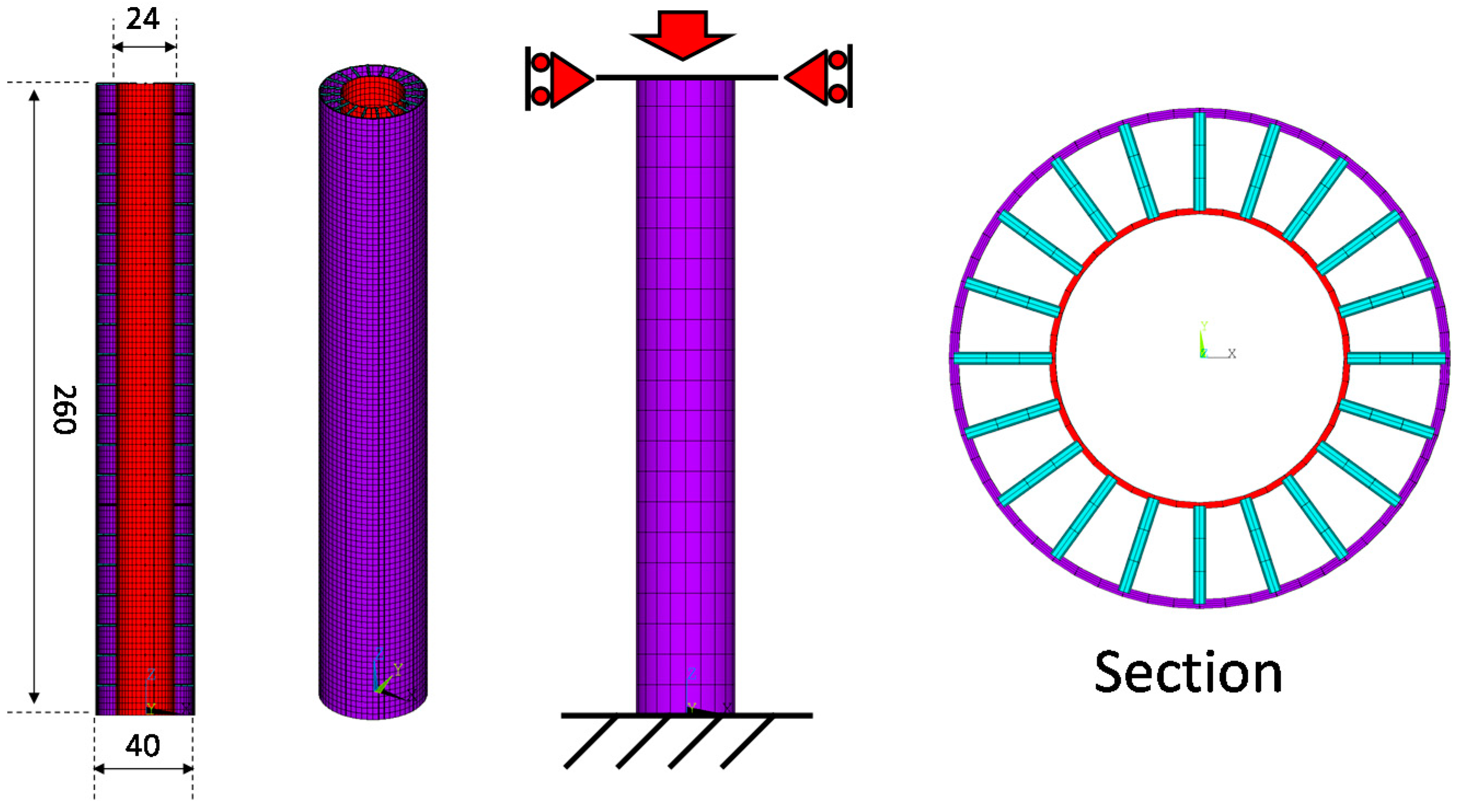
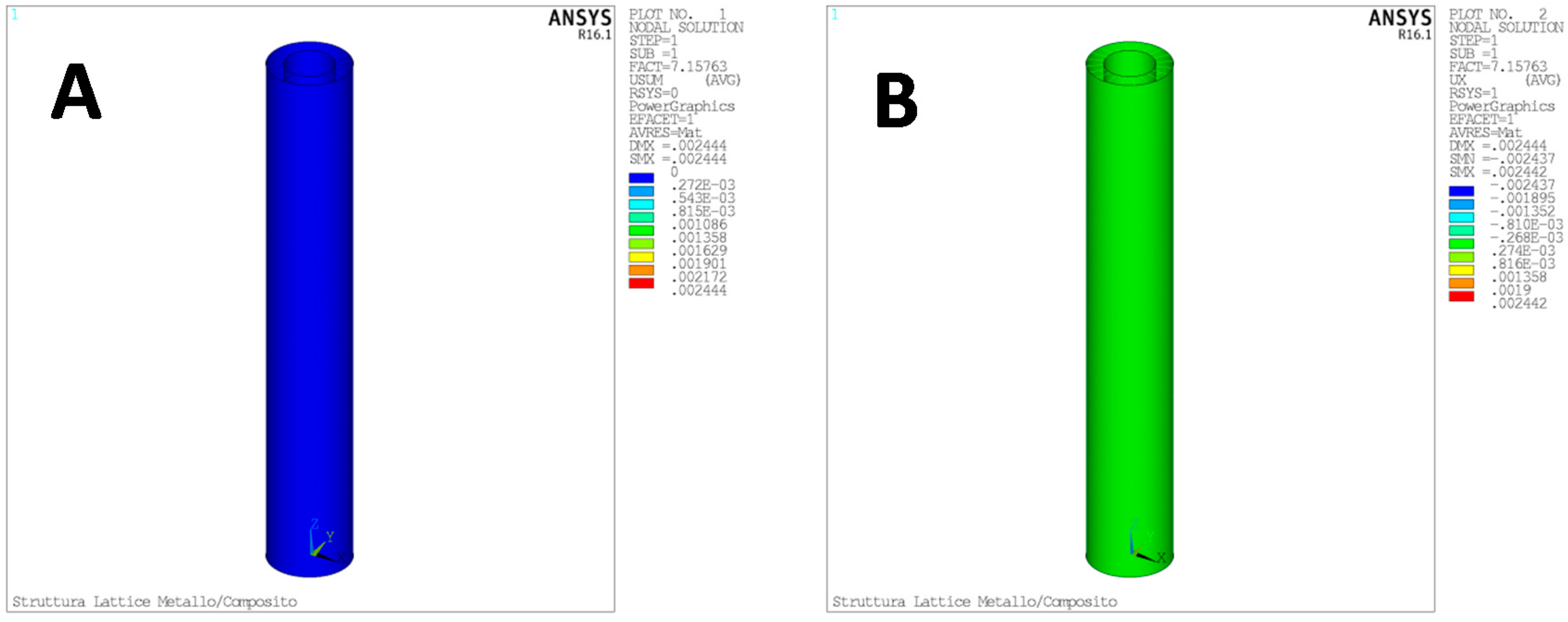
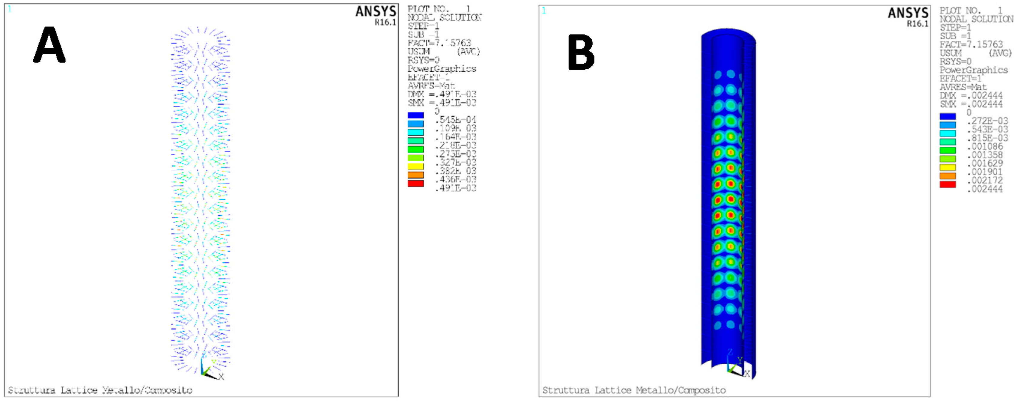
4.1. Test Case 1
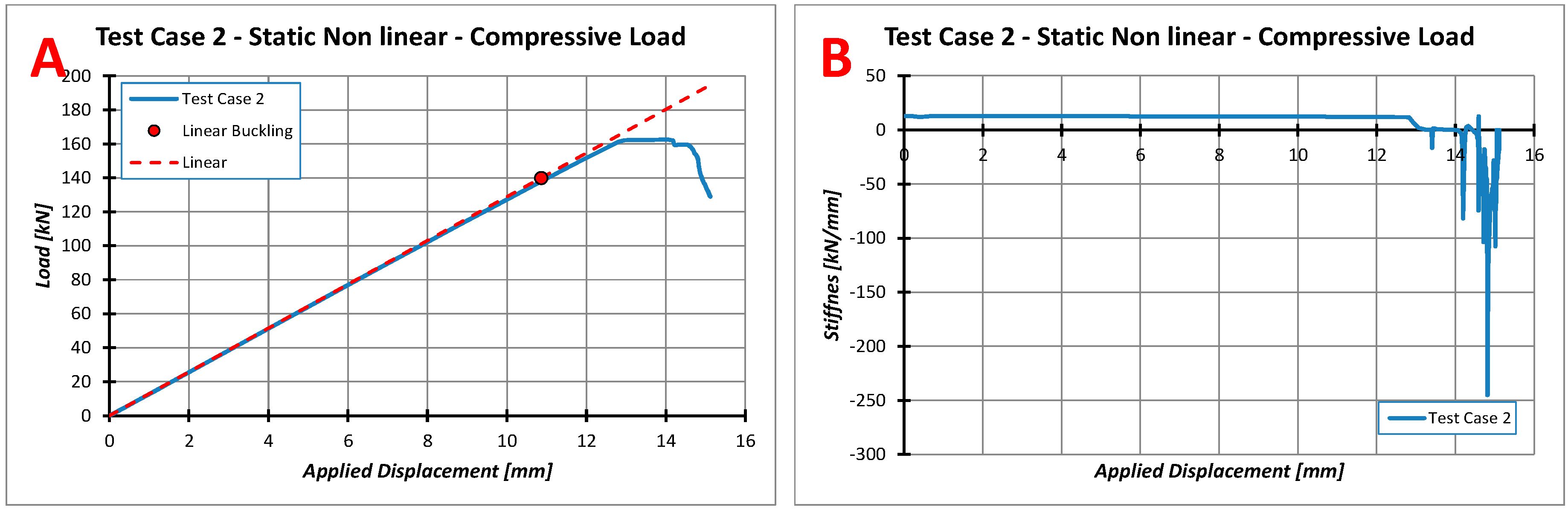
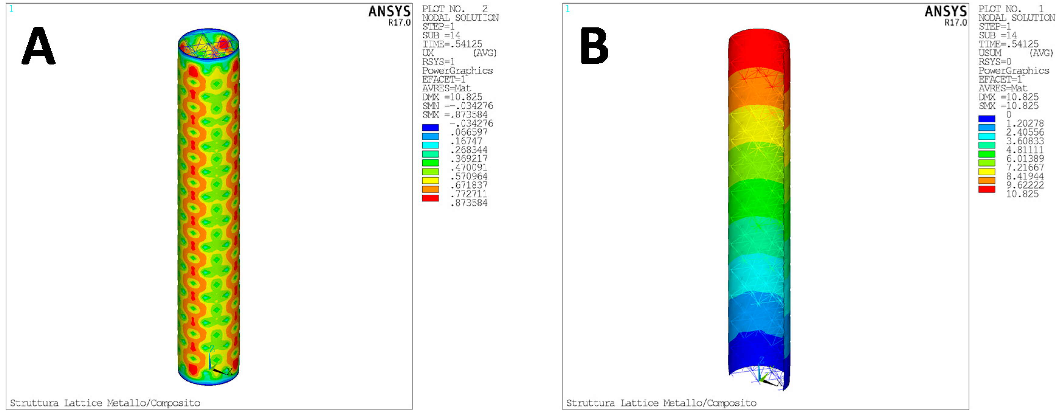
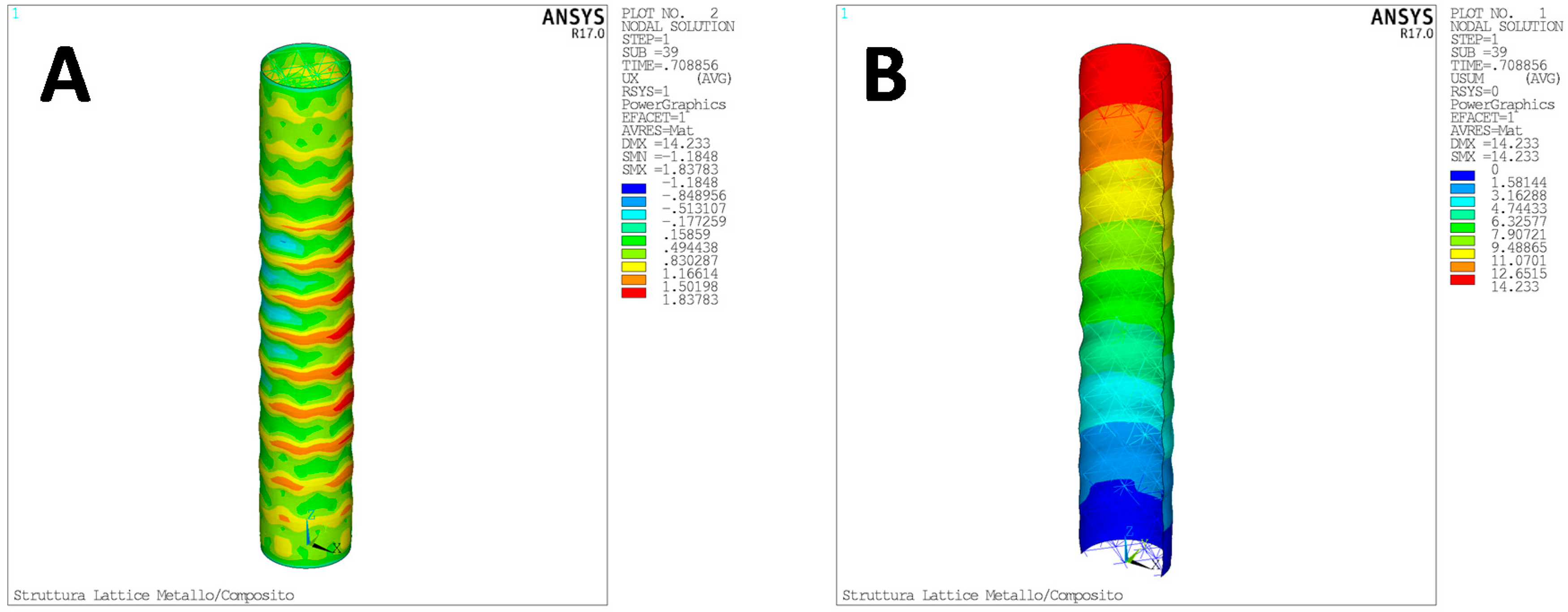
4.2. Test Case 2
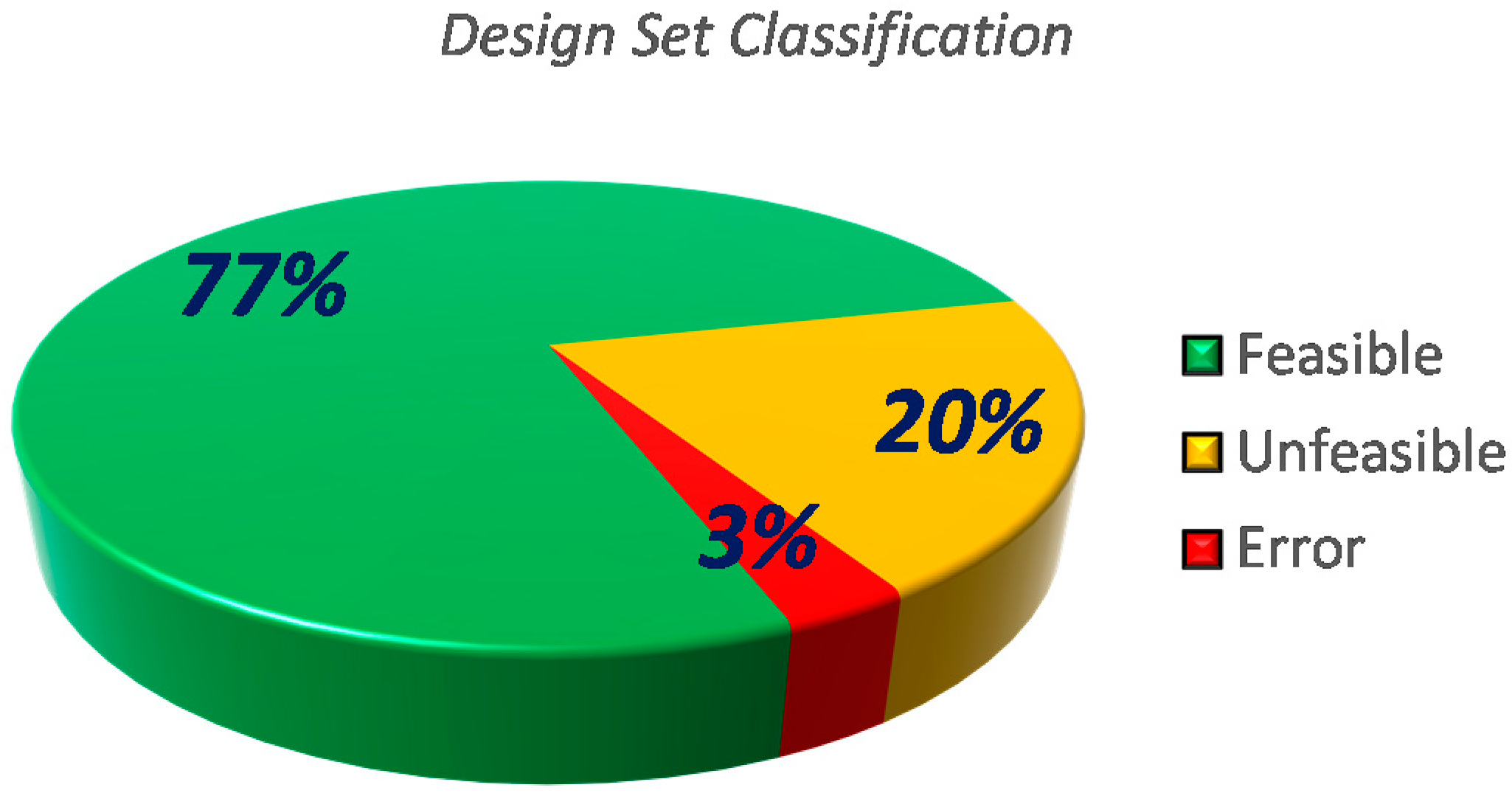
4.3. Test Case 3—Structural Optimization
5. Conclusions
Author Contributions
Funding
Conflicts of Interest
References
- Tofail, S.A.; Koumoulos, E.P.; Bandyopadhyay, A.; Bose, S.; O’Donoghue, L.; Charitidis, C. Additive manufacturing: Scientific and technological challenges, market uptake and opportunities. Mater. Today 2018, 21, 22–37. [Google Scholar] [CrossRef]
- Berman, B. 3-D printing: The new industrial revolution. Bus. Horiz. 2012, 55, 155–162. [Google Scholar] [CrossRef]
- Wohlers, T. Wohlers Report 2014: Global Reports; Wohlers Associates: Fort Collins, CO, USA, 2014. [Google Scholar]
- Wohlers, T. Wohlers Report 2015: Global Reports; Wohlers Associates: Fort Collins, CO, USA, 2015. [Google Scholar]
- Levy, G.N.; Schindel, R.; Kruth, J.P. Rapid manufacturing and rapid tooling with layer manufacturing (LM) technologies, state of the art and future perspectives. CIRP Ann. 2003, 52, 589–609. [Google Scholar] [CrossRef]
- Huang, S.H.; Liu, P.; Mokasdar, A.; Hou, L. Additive manufacturing and its societal impact: A literature review. Int. J. Adv. Manuf. Technol. 2013, 67, 1191–1203. [Google Scholar] [CrossRef]
- Gao, W.; Zhang, Y.; Ramanujan, D.; Ramani, K.; Chen, Y.; Williams, C.B.; Wang, C.C.L.; Shin, Y.C.; Zhang, S.; Zavattieri, P.D. The status, challenges, and future of additive manufacturing in engineering. CAD Comput. Aided Des. 2015, 69, 65–89. [Google Scholar] [CrossRef]
- Herzog, D.; Seyda, V.; Wycisk, E.; Emmelmann, C. Additive manufacturing of metals. Acta Mater. 2016, 117, 371–392. [Google Scholar] [CrossRef]
- Olakanmi, E.; Cochrane, R.; Dalgarno, K. A review on selective laser sintering/melting (SLS/SLM) of aluminium alloy powders: Processing, microstructure, and properties. Prog. Mater. Sci. 2015, 74, 401–447. [Google Scholar] [CrossRef]
- Thompson, M.K.; Moroni, G.; Vaneker, T.; Fadel, G.; Campbell, R.I.; Gibson, I.; Bernard, A.; Schulz, J.; Graf, P.; Ahuja, B.; et al. Design for Additive Manufacturing: Trends, opportunities, considerations, and constraints. CIRP Ann. Manuf. Technol. 2016, 65, 737–760. [Google Scholar] [CrossRef]
- Dilberoglu, U.M.; Gharehpapagh, B.; Yaman, U.; Dolen, M. The role of additive manufacturing in the era of industry 4.0. Procedia Manuf. 2017, 11, 545–554. [Google Scholar] [CrossRef]
- Wu, P.; Wang, J.; Wang, X. A critical review of the use of 3-D printing in the construction industry. Autom. Constr. 2016, 68, 21–31. [Google Scholar] [CrossRef] [Green Version]
- ASTMF2792-12a. Standard Terminology for Additive Manufacturing Technologies; ASTM International: West Conshohocken, PA, USA, 2012. [Google Scholar]
- Gibson, I.; Rosen, D.W.; Stucker, B. Additive Manufacturing Technologies: Rapid Prototyping to Direct Digital Manufacturing; Springer: New York, NY, USA, 2010. [Google Scholar]
- Grenda, E. Printing the Future: The 3D Printing and Rapid Prototyping Sourcebook, 3rd ed.; Castle Island Co.: Arlington, MA, USA, 2009. [Google Scholar]
- Kruth, J.P. Material Increase Manufacturing by Rapid Prototyping Techniques. CIRP Ann. Manuf. Technol. 1991, 40, 603–614. [Google Scholar] [CrossRef]
- Bhushan, B.; Caspers, M. An overview of additive manufacturing (3D printing) for microfabrication. Microsyst. Technol. 2017, 23, 1117–1124. [Google Scholar] [CrossRef]
- Panesar, A.; Abdi, M.; Hickman, D.; Ashcroft, I. Strategies for functionally graded lattice structures derived using topology optimisation for additive manufacturing. Addit. Manuf. 2018, 19, 81–94. [Google Scholar] [CrossRef]
- Ngo, T.D.; Kashani, A.; Imbalzano, G.; Nguyen, K.T.Q.; Hui, D. Additive manufacturing (3D printing): A review of materials, methods, applications and challenges. Compos. Part B Eng. 2018, 143, 172–196. [Google Scholar] [CrossRef]
- Brooks, H.; Brigden, K. Design of conformal cooling layers with self-supporting lattices for additively manufactured tooling. Addit. Manuf. 2016, 11, 16–22. [Google Scholar] [CrossRef] [Green Version]
- Gu, D.D.; Meiners, W.; Wissenbach, K.; Poprawe, R. Laser additive manufacturing of metallic components: Materials, processes and mechanisms. Int. Mater. Rev. 2012, 57, 133–164. [Google Scholar] [CrossRef]
- Chua, C.K.; Leong, K.F.; Lim, C.S. Innovative Developments in Design and Manufacturing—Advanced Research in Virtual and Rapid Prototyping. In Rapid Prototyping: Principles and Applications, 3rd ed.; World Scientific Publishing Co Pte Ltd: Singapore, 2010; pp. 497–503. [Google Scholar]
- Lee, H.; Lim, C.H.J.; Low, M.J.; Tham, N.; Murukeshan, V.M.; Kim, Y.-J. Lasers in additive manufacturing: A review. Int. J. Precis. Eng. Manuf. Green Technol. 2017, 4, 307–322. [Google Scholar] [CrossRef]
- Mure, L.E.; Gaytan, S.M.; Ramirez, D.A.; Martines, E.; Hernandez, J.; Amato, K.N.; Shindo, P.W.; Medina, F.R.; Wicker, R.B. Metal Fabrication by Additive Manufacturing Using Laser and Electron Beam Melting Technologies. J. Mater. Sci. Technol. 2012, 28, 1–14. [Google Scholar] [CrossRef]
- Rafi, H.K.; Karthik, N.V.; Gong, H.; Starr, T.L.; Stucker, B.E. Microstructures and mechanical properties of Ti6Al4V parts fabricated by selective laser melting and electron beam melting. J. Mater. Eng. Perform. 2013, 22, 3872–3883. [Google Scholar] [CrossRef]
- Sing, S.L.; An, J.; Yeong, W.Y.; Wiria, F.E. Laser and electron-beam powder-bed additive manufacturing of metallic implants: A review on processes, materials and designs. J. Orthop. Res. 2016, 34, 369–385. [Google Scholar] [CrossRef]
- Biamino, S.; Penna, A.; Ackelid, U.; Sabbadini, S.; Tassa, O.; Fino, P.; Pavese, M.; Gennaro, P.; Badini, C. Electron beam melting of Ti-48Al-2Cr-2Nb alloy: Microstructure and mechanical properties investigation. Intermetallics 2011, 19, 776–781. [Google Scholar] [CrossRef]
- Tomlin, M.; Meyer, J. Topology optimization of an additive layer manufactured (ALM) aerospace part. In Proceedings of the 7th Altair CAE Technology Conference, Warwickshire, UK, 10 May 2011. [Google Scholar]
- Krog, L.; Tucker, A.; Rollema, G. Application of topology, sizing and shape optimization methods to optimal design of aircraft components. In Proceedings of the 3rd Altair UK HyperWorks Users Conference, Coventry, UK, 11–12 November 2002. [Google Scholar]
- Ferguson, I.; Frecker, M.; Simpson, T.W. Topology optimization software for additive manufacturing: A review of current capabilities and a real-world example. In Proceedings of the ASME 2016 International Design Engineering Technical Conferences and Computers and Information in Engineering Conference, Charlotte, CA, USA, 21–24 August 2016; American Society of Mechanical Engineers: New York, NY, USA, 2016. [Google Scholar]
- Saadlaoui, Y.; Milan, J.-L.; Rossi, J.-M.; Chabrand, P. Topology optimization and additive manufacturing: Comparison of conception methods using industrial codes. J. Manuf. Syst. 2017, 43, 178–186. [Google Scholar] [CrossRef]
- Chen, W.; Zheng, X.; Liu, S. Finite-Element-Mesh Based Method for Modeling and Optimization of Lattice Structures for Additive Manufacturing. Materials 2018, 11, 2073. [Google Scholar] [CrossRef] [PubMed]
- Mahmoud, D.; Elbestawi, M.A. Lattice Structures and Functionally Graded Materials Applications in Additive Manufacturing of Orthopedic Implants: A Review. J. Manuf. Mater. Process. 2017, 1, 13. [Google Scholar] [CrossRef]
- Jiang, J.; Xu, X.; Stringer, J. Support Structures for Additive Manufacturing: A Review. J. Manuf. Mater. Process. 2018, 2, 64. [Google Scholar] [CrossRef]
- Ferro, C.G.; Varetti, S.; Vitti, F.; Maggiore, P.; Lombardi, M.; Biamino, S.; Manfredi, D.; Calignano, F. A Robust Multifunctional Sandwich Panel Design with Trabecular Structures by the Use of Additive Manufacturing Technology for a New De-Icing System. Technologies 2017, 5, 35. [Google Scholar] [CrossRef]
- Cooper, K.; Steele, P.; Cheng, B.; Chou, K. Contact-Free Support Structures for Part Overhangs in Powder-Bed Metal Additive Manufacturing. Inventions 2018, 3, 2. [Google Scholar] [CrossRef]
- Williams, C.B.; Cochran, J.K.; Rosen, D.W. Additive manufacturing of metallic cellular materials via three-dimensional printing. Int. J. Adv. Manuf. Technol. 2011, 53, 231–239. [Google Scholar] [CrossRef]
- Rosen, D.W. Computer-aided design for additive manufacturing of cellular structures. Comput. Aided Des. Appl. 2007, 4, 585–594. [Google Scholar] [CrossRef]
- Deshpande, V.S.; Fleck, N.A.; Ashby, M.F. Effective properties of the octet-truss lattice material. J. Mech. Phys. Solids 2001, 49, 1747–1769. [Google Scholar] [CrossRef] [Green Version]
- Zhang, Y.; Bernard, A.; Gupta, R.K.; Harik, R. Evaluating the design for additive manufacturing: A process planning perspective. Procedia CIRP 2014, 21, 144–150. [Google Scholar] [CrossRef]
- Riccio, A.; Raimondo, F.; Sellitto, A.; Carandente, V.; Scigliano, R.; Tescione, D. Optimum design of ablative thermal protection systems for atmospheric entry vehicles. Appl. Therm. Eng. 2017, 119, 541–552. [Google Scholar] [CrossRef]
- Vaissier, B.; Pernot, J.-P.; Chougrani, L.; Véron, P. Genetic-algorithm based framework for lattice support structure optimization in additive manufacturing. CAD Comput. Aided Des. 2018, 110, 11–23. [Google Scholar] [CrossRef]
- Sellitto, A.; Borrelli, R.; Caputo, F.; Riccio, A.; Scaramuzzino, F. Application to plate components of a kinematic global-local approach for non-matching finite element meshes. Int. J. Struct. Integr. 2012, 3, 260–273. [Google Scholar] [CrossRef]
- Sellitto, A.; Borrelli, R.; Caputo, F.; Riccio, A.; Scaramuzzino, F. Methodological approaches for kinematic coupling of non-matching finite element meshes. Procedia Eng. 2011, 10, 421–426. [Google Scholar] [CrossRef]
- Ferrigno, A.; Di Caprio, F.; Borrelli, R.; Auricchio, F.; Vigliotti, A. The mechanical strength of Ti-6Al-4V columns with regular octet microstructure manufactured by electron beam melting. Materialia 2019, 5. [Google Scholar] [CrossRef]
- Ahmadi, S.; Campoli, G.; Yavari, S.A.; Sajadi, B.; Wauthle, R.; Schrooten, J.; Weinans, H.; Zadpoor, A. Mechanical behavior of regular open-cell porous biomaterials made of diamond lattice unit cells. J. Mech. Behav. Biomed. Mater. 2014, 34, 106–115. [Google Scholar] [CrossRef]
- Dong, L.; Wadley, H. Mechanical properties of carbon fiber composite octet-truss lattice structures. Compos. Sci. Technol. 2015, 119, 26–33. [Google Scholar] [CrossRef]


| Connection ID | Connection Flag 0 = Not Active 1 = Active | Node 1 | Node 2 |
|---|---|---|---|
| 1 | 1 | 1 | 2 |
| 2 | 0 | 1 | 3 |
| 3 | 1 | 2 | 4 |
| … | … | … | … |
| 28 | 0 | 4 | 8 |
| Lattice Mass | External Skin Mass | Internal Skin Mass | Total Mass |
|---|---|---|---|
| 0.246 (kg) | 0.099 (kg) | 0.262 (kg) | 0.609 (kg) |
| Lattice Mass | External Skin Mass | Internal Skin Mass | Total Mass |
|---|---|---|---|
| 0.098 (kg) | 0.058 (kg) | N/A | 0.157 (kg) |
| UC_RAD1 | UC_L1z | UC_L1TH | UC_NSYS2 | NPLY | SKIN_INT_TH | Connect_2X Matrix |
|---|---|---|---|---|---|---|
| radius single connecting element | cell size in axial direction | N° of cells in tangential direction | N° of cells in the thickness (between internal and external skin) | N° of ply of external skin | thickness of metallic internal skin | 28 connection flags for 8-node cell. |
| Lattice Mass | External Skin Mass | Internal Skin Mass | Total Mass |
|---|---|---|---|
| 0.011 (kg) | 0.038 (kg) | 0.043 (kg) | 0.0936 (kg) |
| Section Radius (mm) | Section Diameter (mm) | Inertia Section (mm4) | Length (mm) | Young’s Module (MPa) | Density (Ton/mm3) | Volume (mm3) | Mass (kg) | Critical Load (kN) |
|---|---|---|---|---|---|---|---|---|
| 7.60 | 15.21 | 2625.00 | 260.00 | 100,000.00 | 0.00 | 47,209.88 | 0.208 | 143.0 |
© 2019 by the authors. Licensee MDPI, Basel, Switzerland. This article is an open access article distributed under the terms and conditions of the Creative Commons Attribution (CC BY) license (http://creativecommons.org/licenses/by/4.0/).
Share and Cite
Di Caprio, F.; Acanfora, V.; Franchitti, S.; Sellitto, A.; Riccio, A. Hybrid Metal/Composite Lattice Structures: Design for Additive Manufacturing. Aerospace 2019, 6, 71. https://doi.org/10.3390/aerospace6060071
Di Caprio F, Acanfora V, Franchitti S, Sellitto A, Riccio A. Hybrid Metal/Composite Lattice Structures: Design for Additive Manufacturing. Aerospace. 2019; 6(6):71. https://doi.org/10.3390/aerospace6060071
Chicago/Turabian StyleDi Caprio, Francesco, Valerio Acanfora, Stefania Franchitti, Andrea Sellitto, and Aniello Riccio. 2019. "Hybrid Metal/Composite Lattice Structures: Design for Additive Manufacturing" Aerospace 6, no. 6: 71. https://doi.org/10.3390/aerospace6060071