Figure 1.
A-SOFT (Altering-intensity Swirling-Oxidizer-Flow-Type) concept with dual front oxidizer injections [
10].
Figure 1.
A-SOFT (Altering-intensity Swirling-Oxidizer-Flow-Type) concept with dual front oxidizer injections [
10].
Figure 2.
A-SOFT engine simplification for the simulations.
Figure 2.
A-SOFT engine simplification for the simulations.
Figure 3.
Mass flow rate profile in function of the valve opening.
Figure 3.
Mass flow rate profile in function of the valve opening.
Figure 4.
(a) resistor-based sensor principle and (b) modeling.
Figure 4.
(a) resistor-based sensor principle and (b) modeling.
Figure 5.
AOA (Aft-end Oxidizer Addition) concept with front and aft-end oxidizer injections.
Figure 5.
AOA (Aft-end Oxidizer Addition) concept with front and aft-end oxidizer injections.
Figure 6.
Normalized thrust errors.
Figure 6.
Normalized thrust errors.
Figure 7.
Normalized mixture ratio errors.
Figure 7.
Normalized mixture ratio errors.
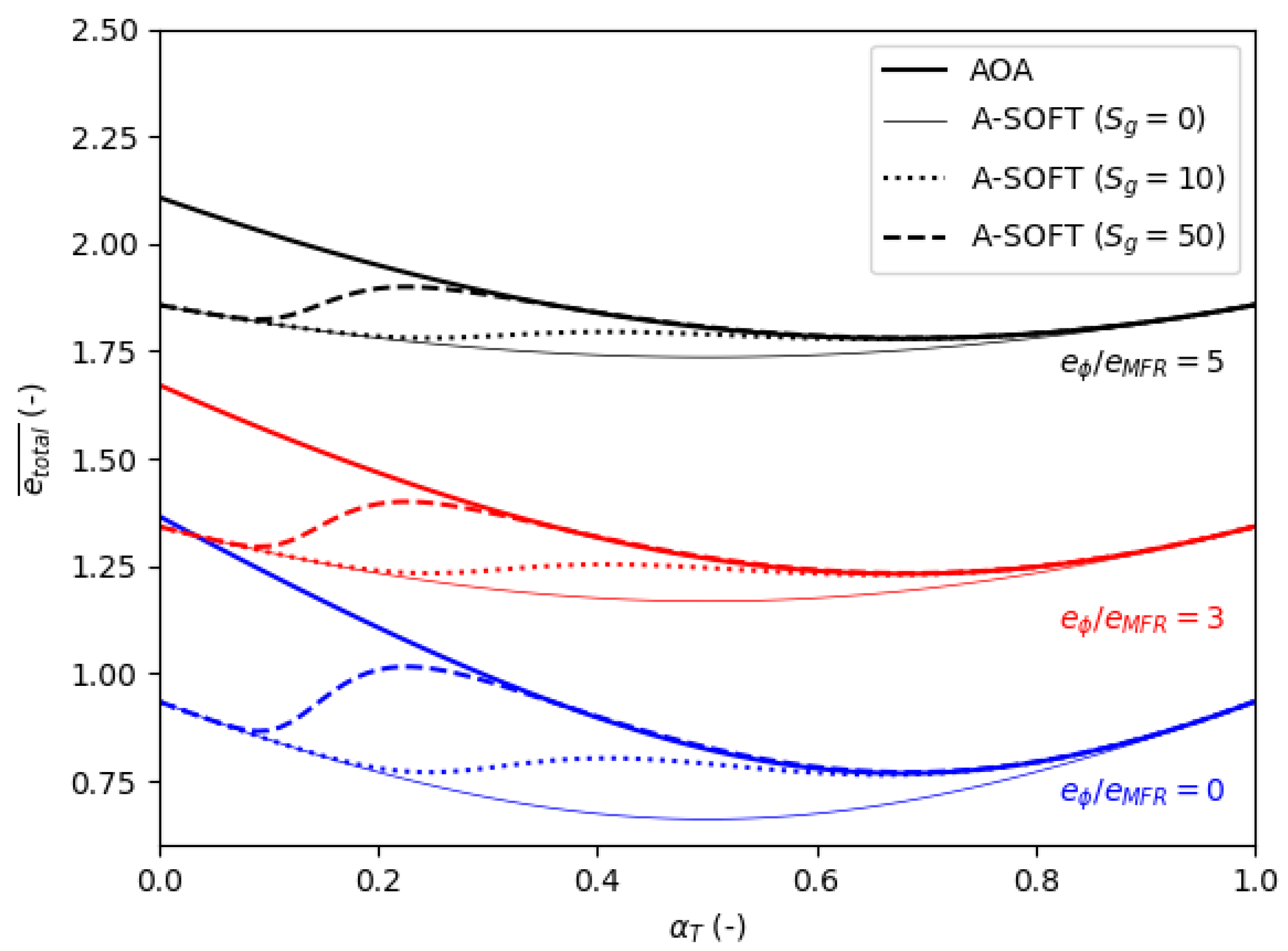
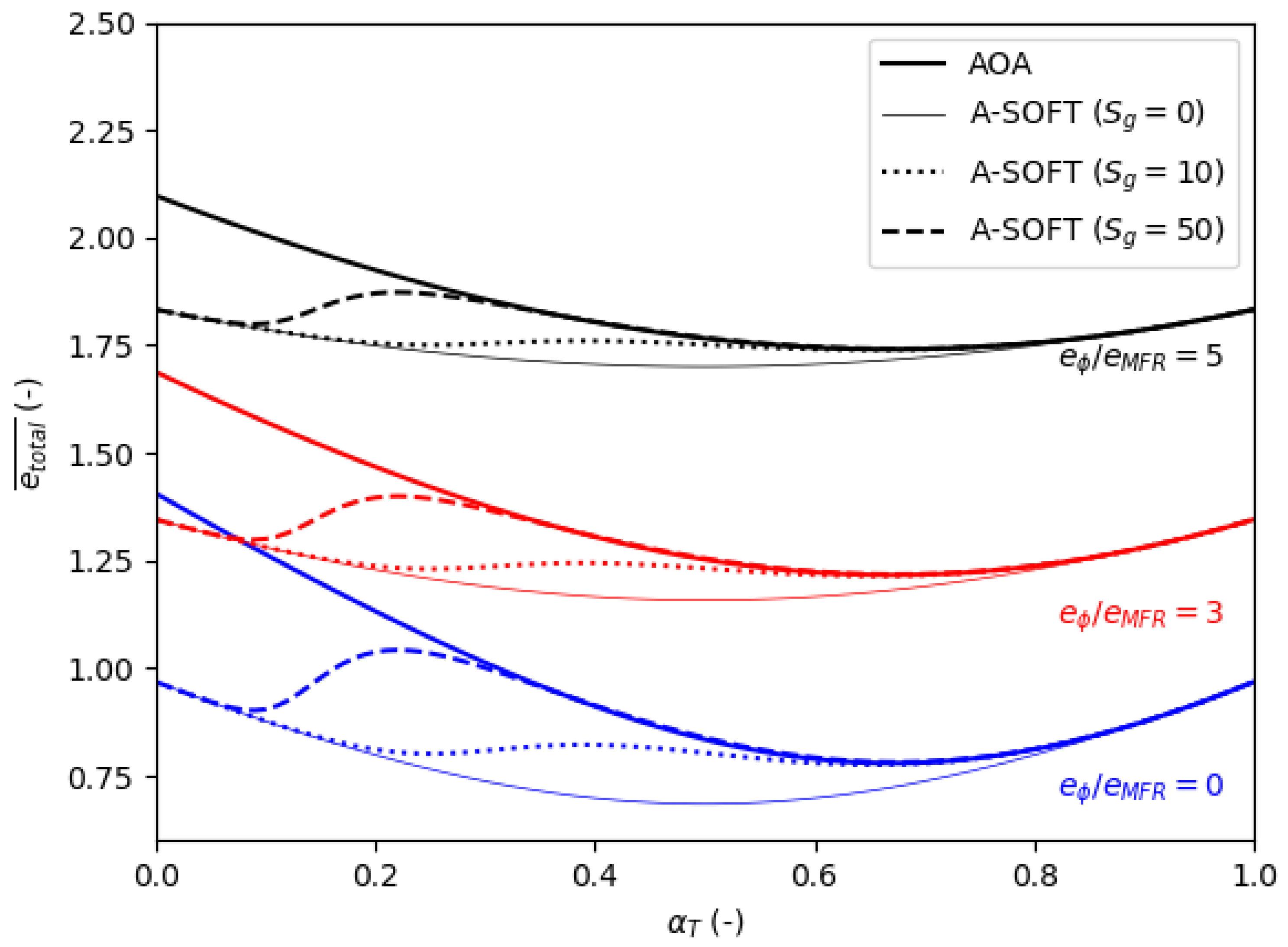
Figure 8.
Normalized total errors.
Figure 8.
Normalized total errors.
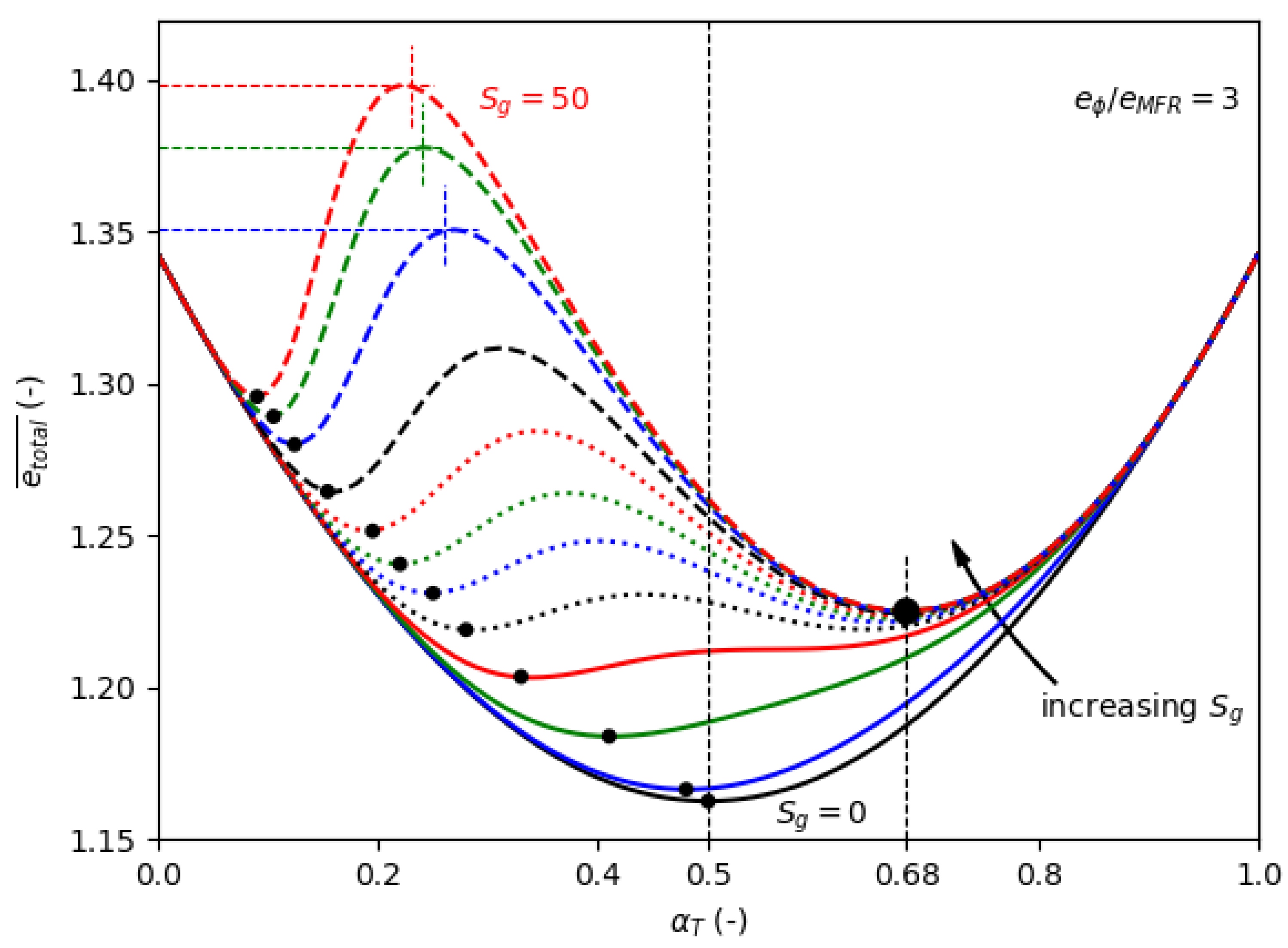
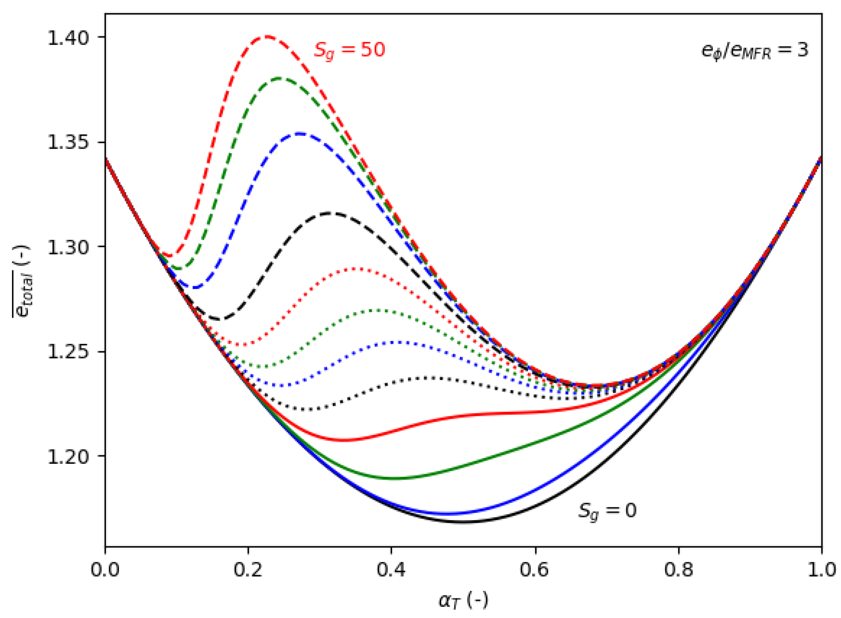
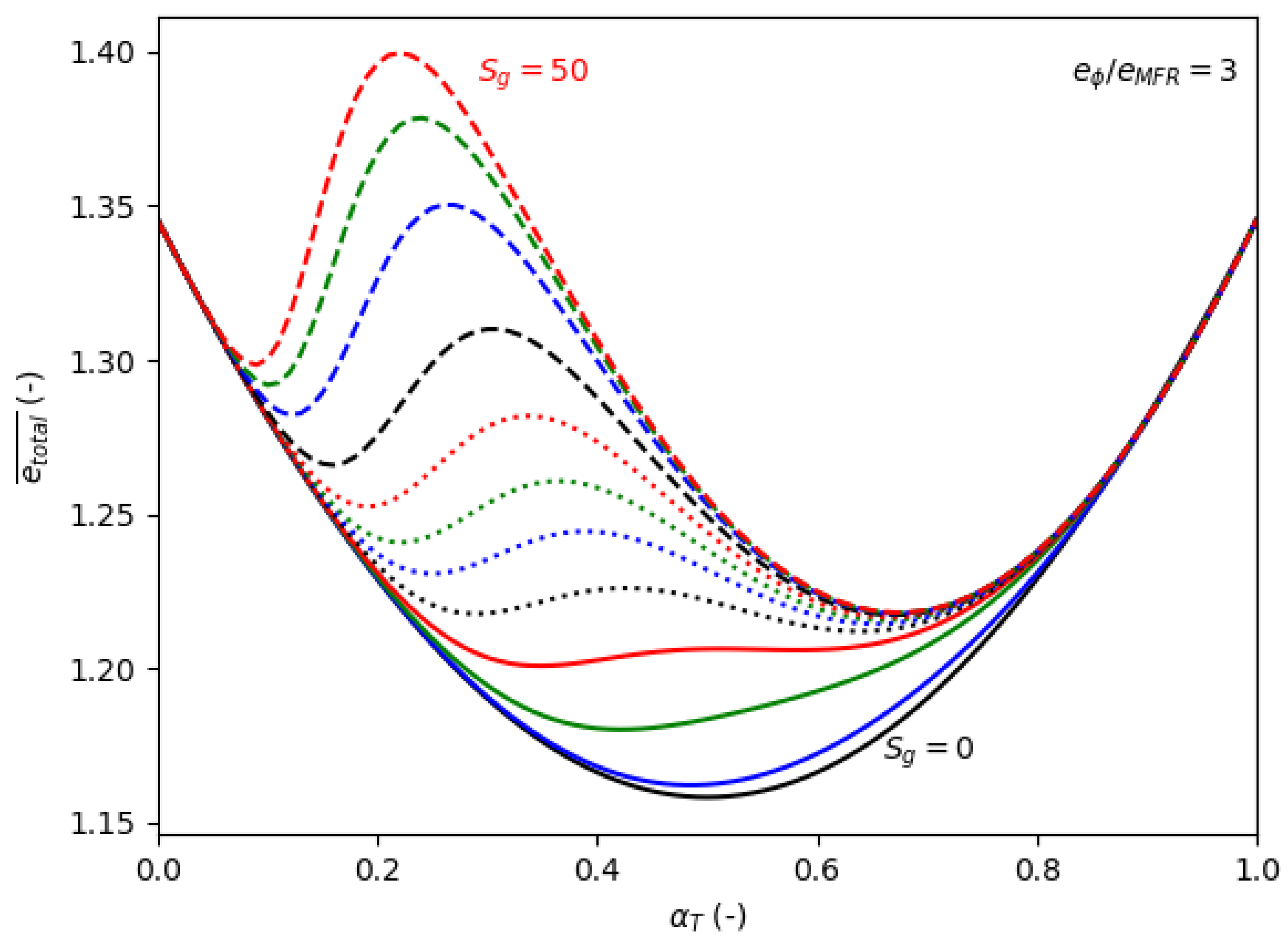
Figure 9.
Influence of the geometric swirl number on the normalized total errors in A-SOFT engines for values in [0,2,4,6,8,10,12,15,20,30,40,50].
Figure 9.
Influence of the geometric swirl number on the normalized total errors in A-SOFT engines for values in [0,2,4,6,8,10,12,15,20,30,40,50].
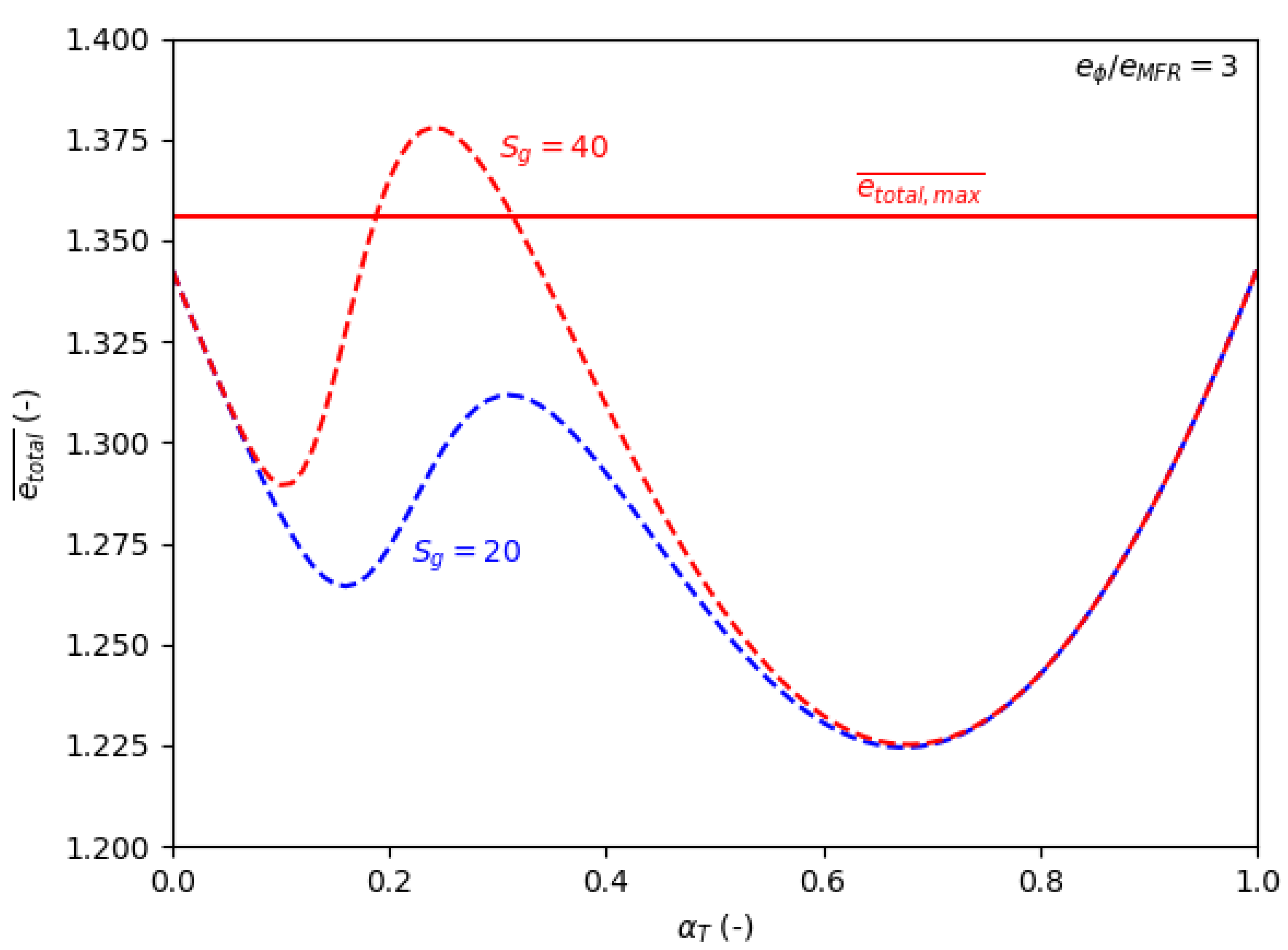
Figure 10.
Illustration of the C1 criterion.
Figure 10.
Illustration of the C1 criterion.
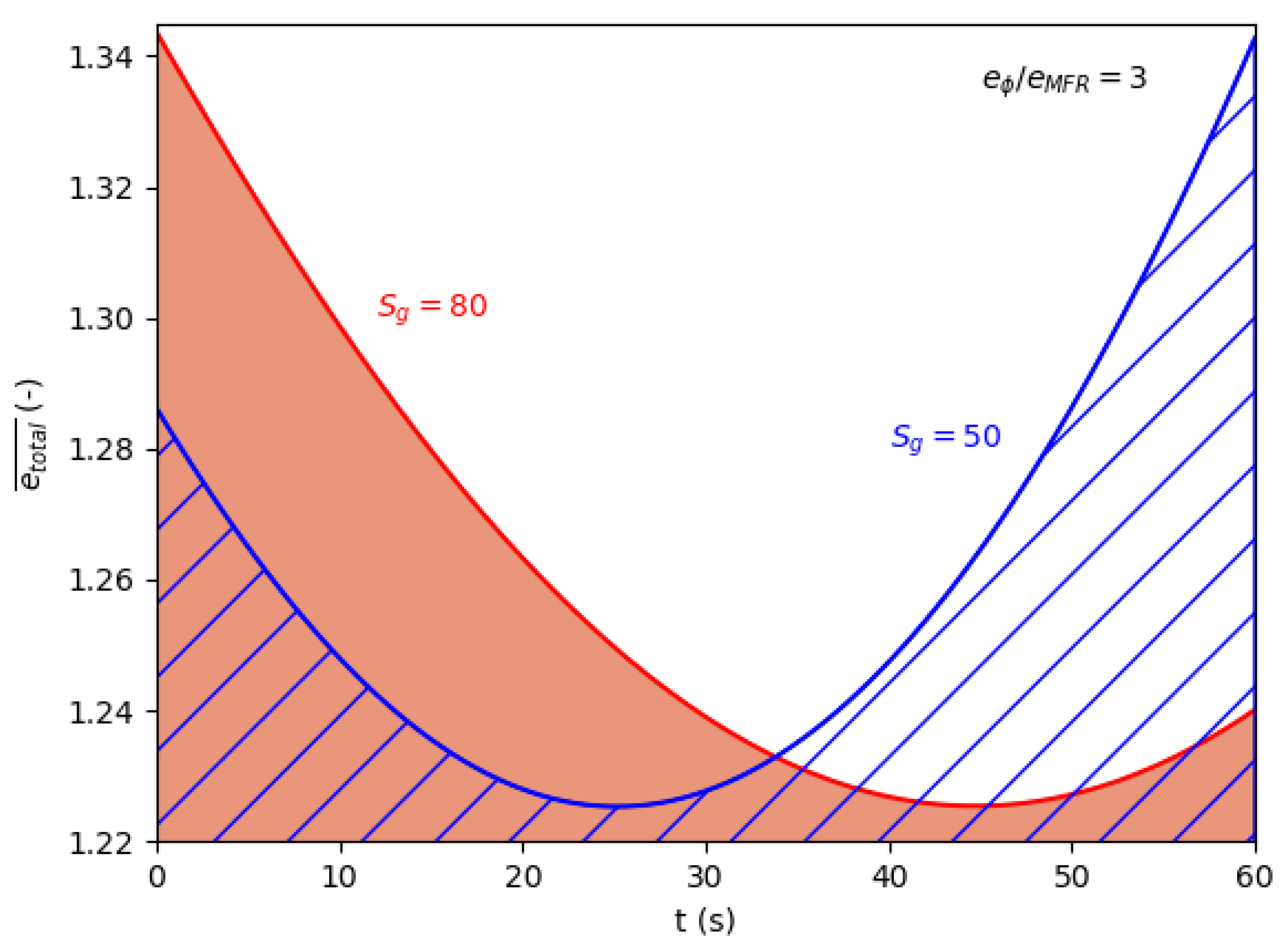
Figure 11.
Illustration of the C2 criterion.
Figure 11.
Illustration of the C2 criterion.
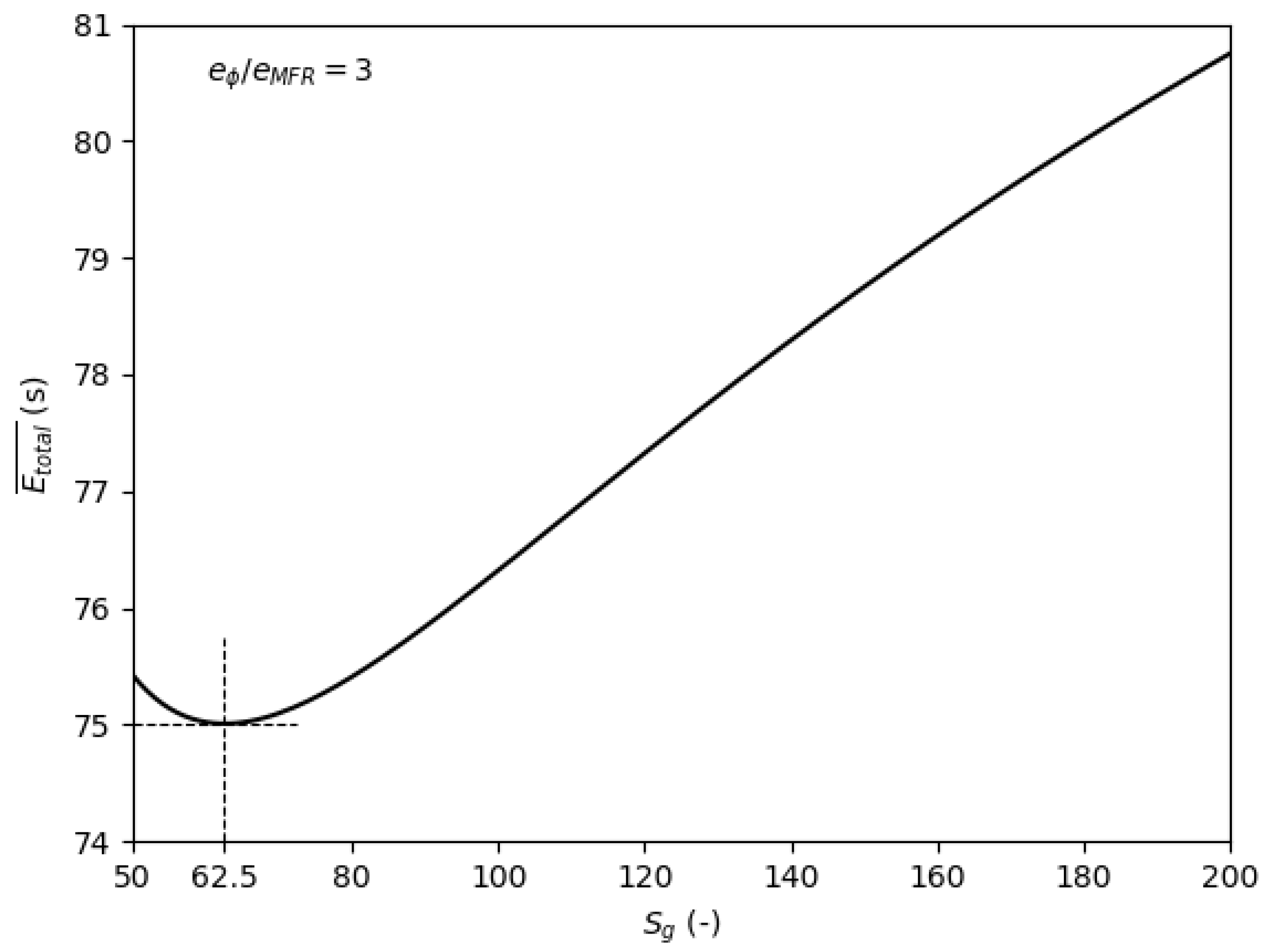
Figure 12.
Integrated error evolution depending on the geometric swirl number.
Figure 12.
Integrated error evolution depending on the geometric swirl number.
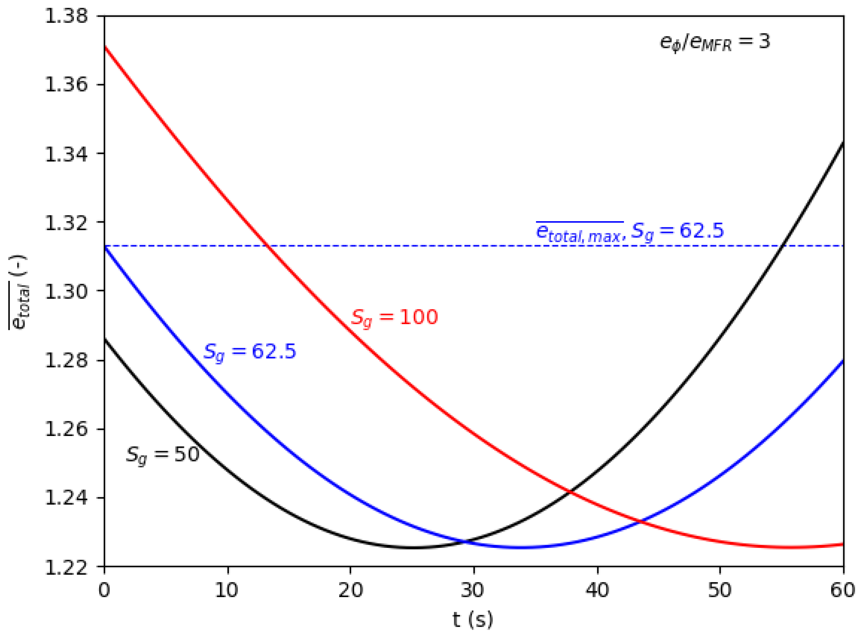
Figure 13.
Instantaneous total error evolution.
Figure 13.
Instantaneous total error evolution.
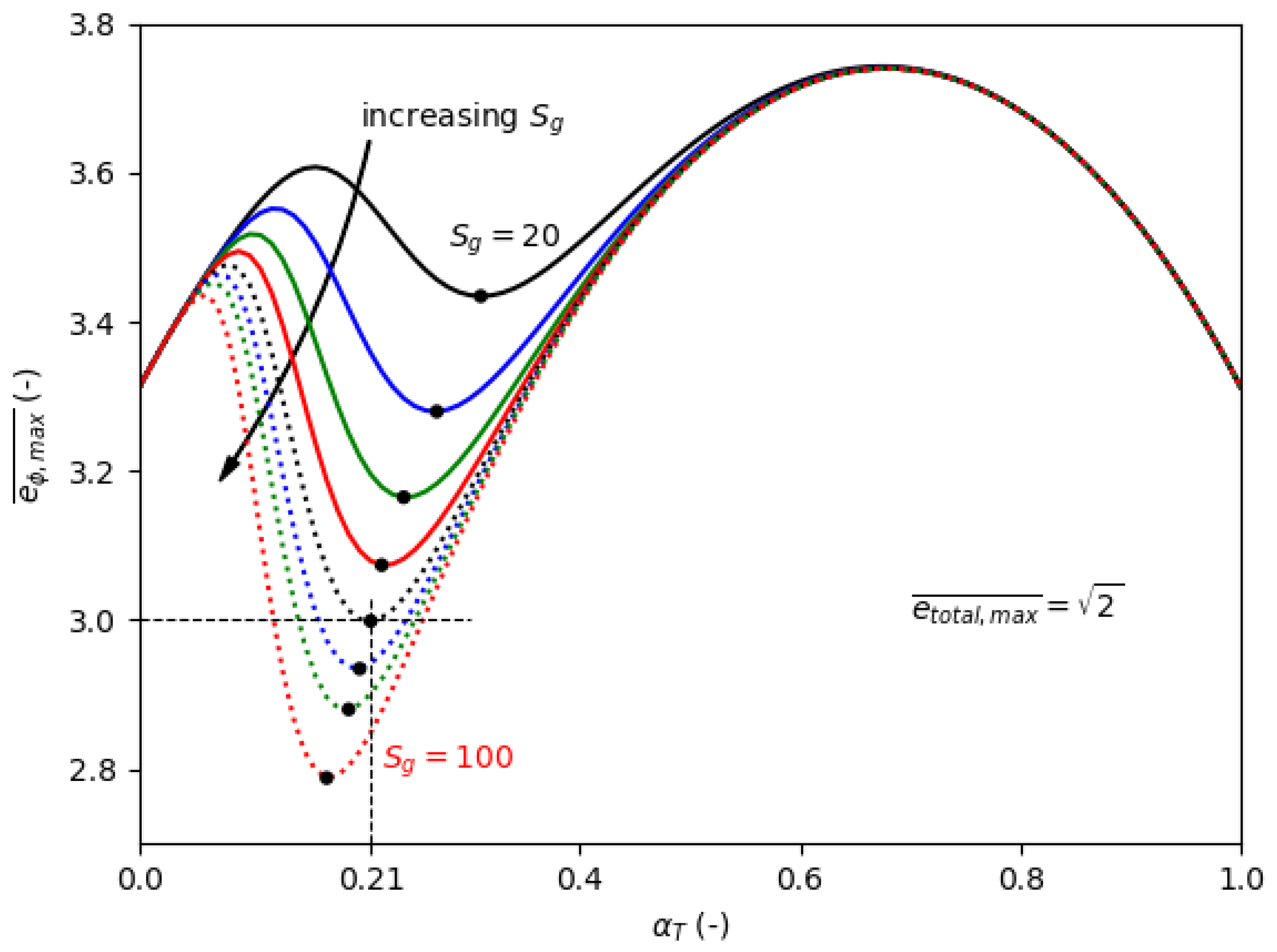
Figure 14.
Maximum normalized diameter error for values in [20,30,40,50,60,70,80,100].
Figure 14.
Maximum normalized diameter error for values in [20,30,40,50,60,70,80,100].
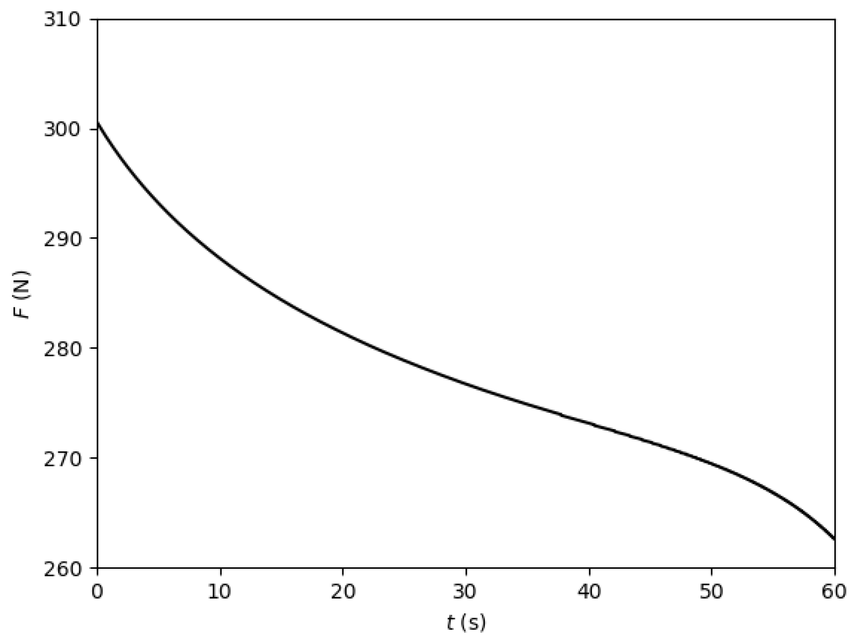
Figure 15.
Thrust profile without feedback control.
Figure 15.
Thrust profile without feedback control.
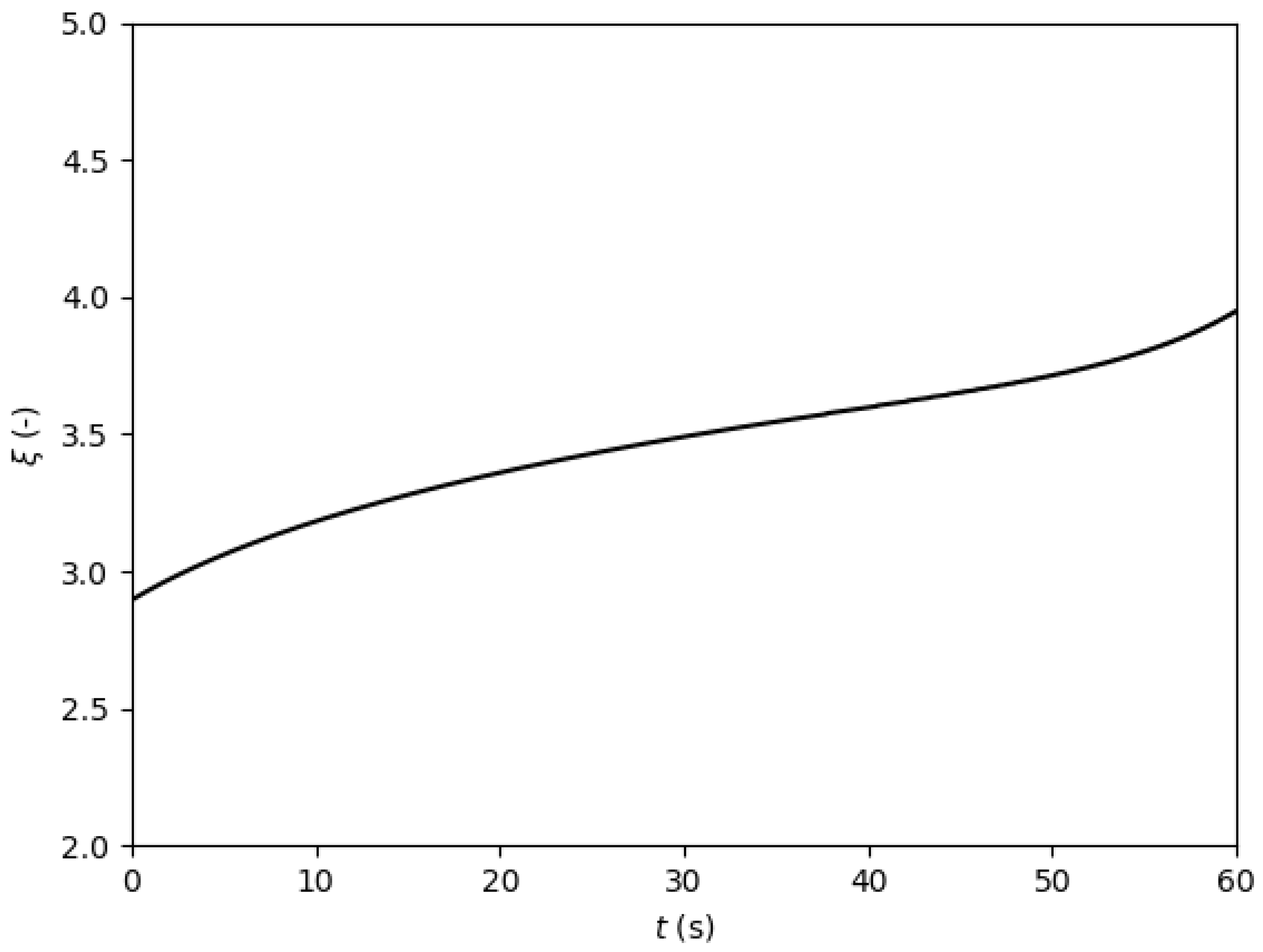
Figure 16.
Mixture ratio profile without feedback control.
Figure 16.
Mixture ratio profile without feedback control.
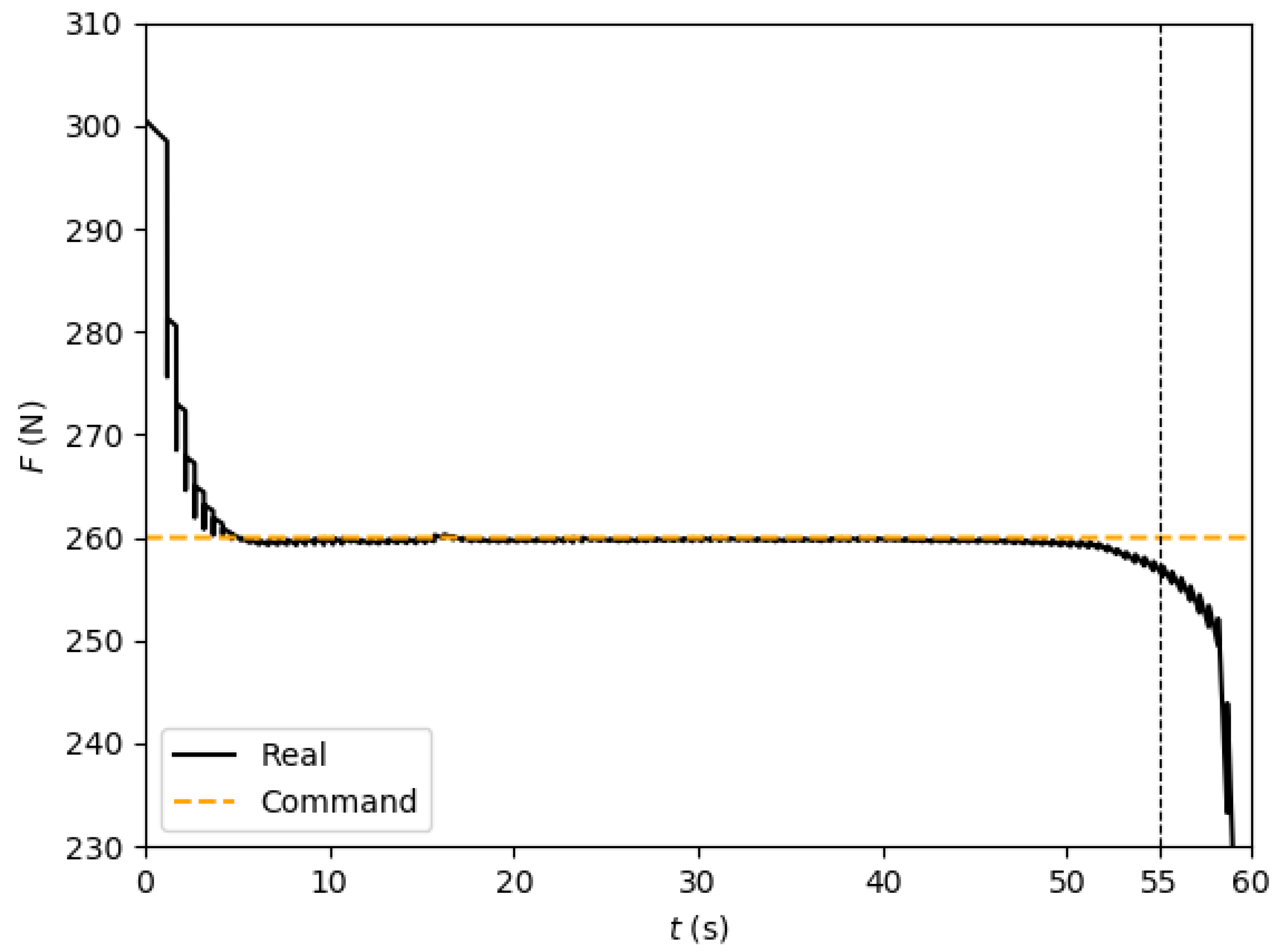
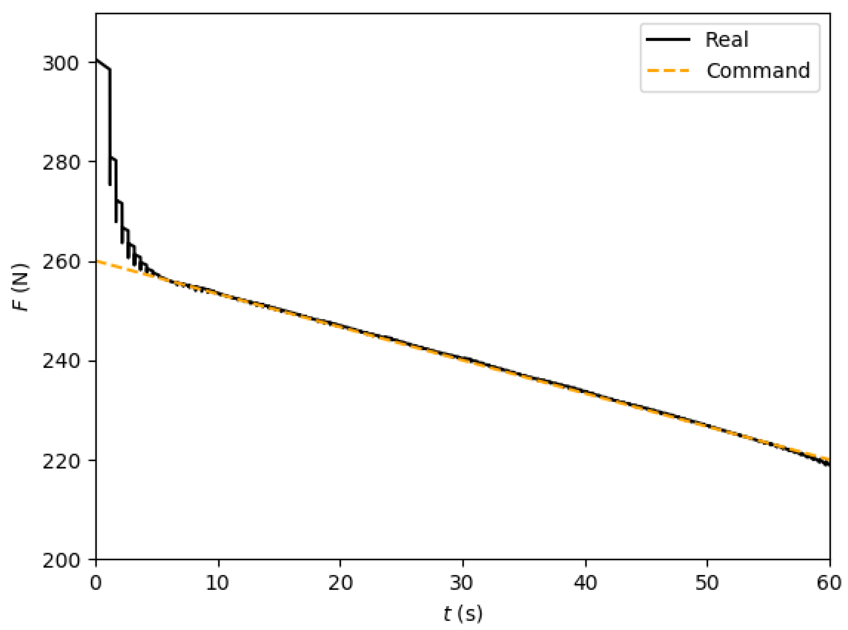
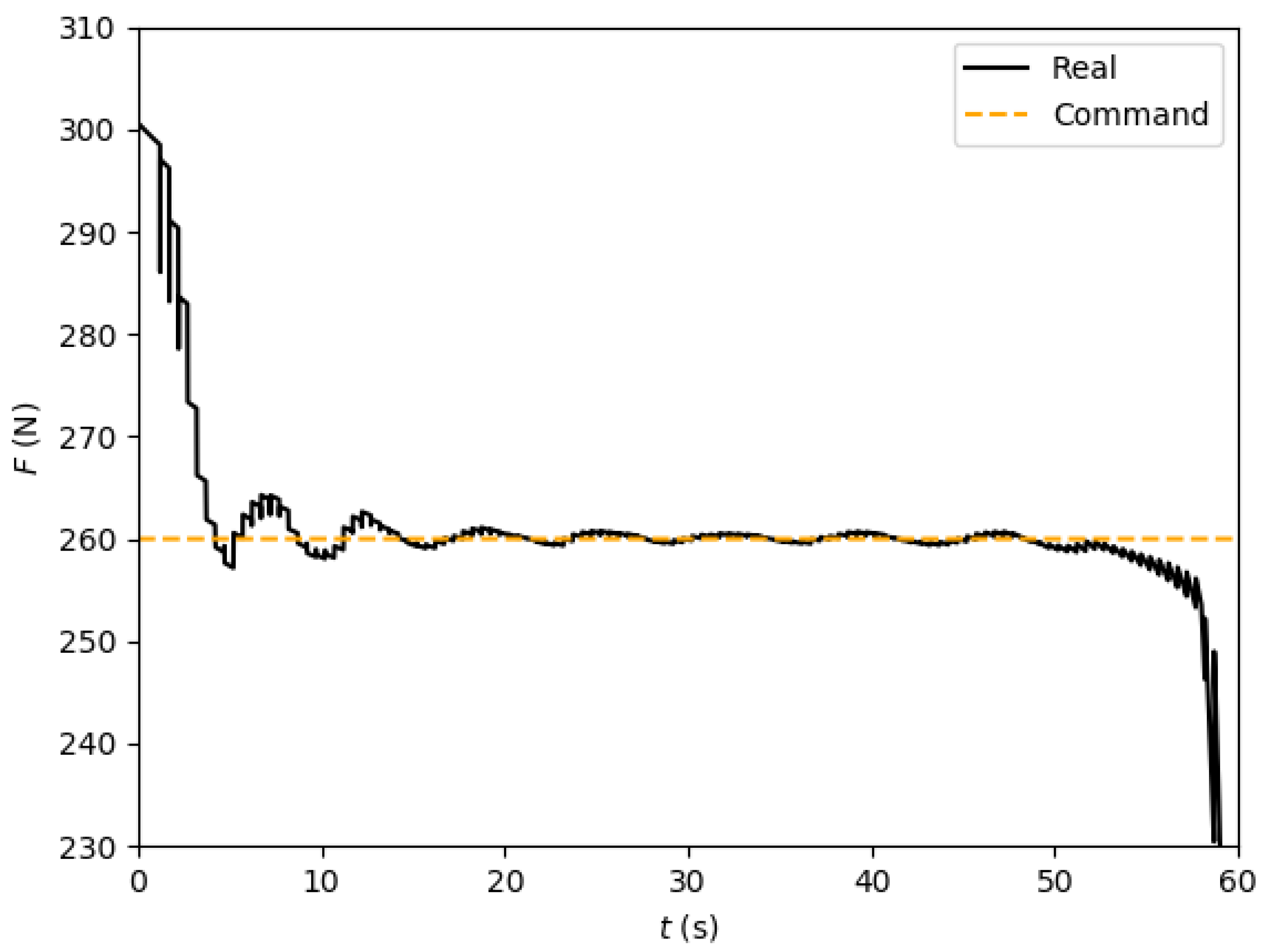
Figure 17.
Thrust profile, feedback with complete regulation law, case 1.
Figure 17.
Thrust profile, feedback with complete regulation law, case 1.
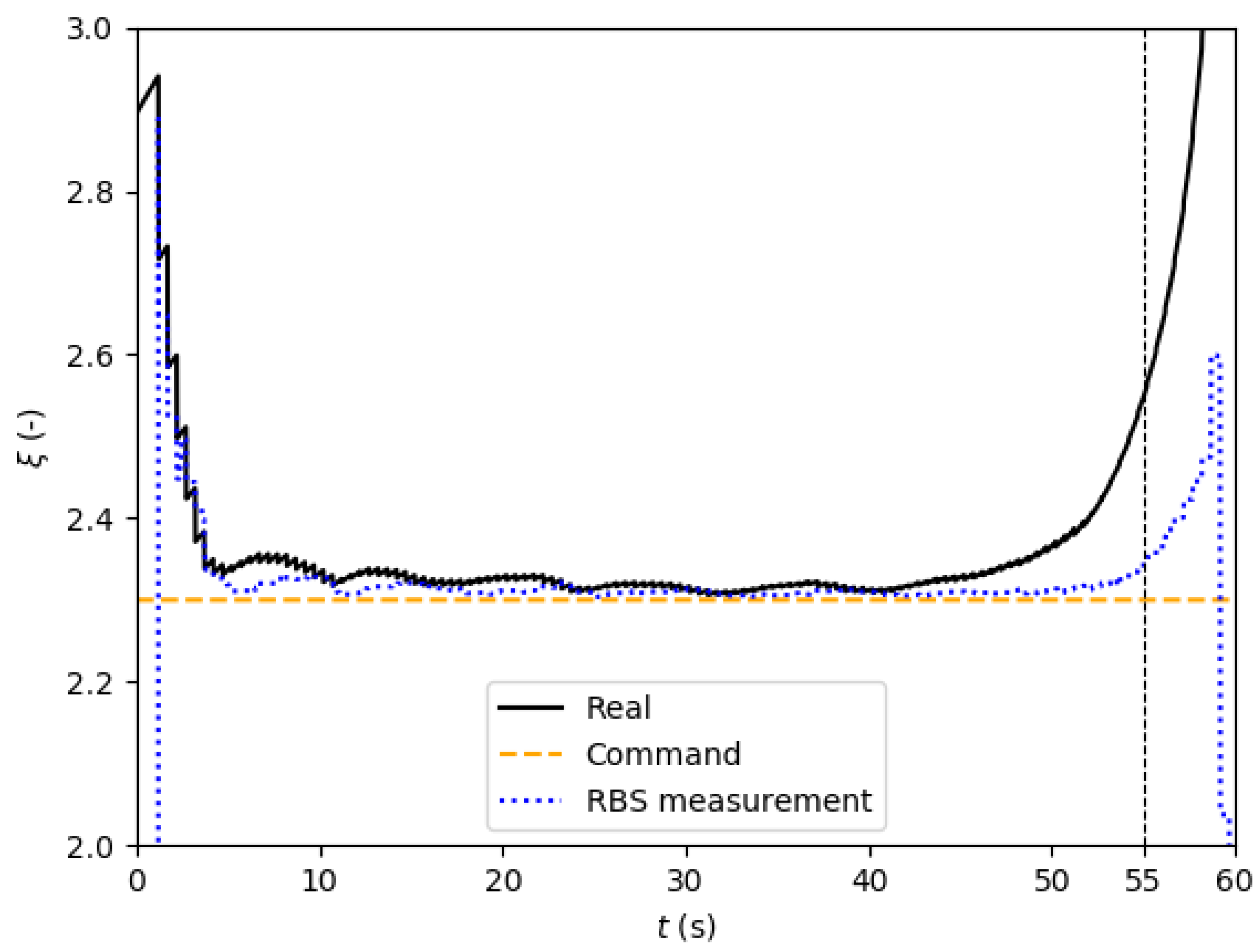
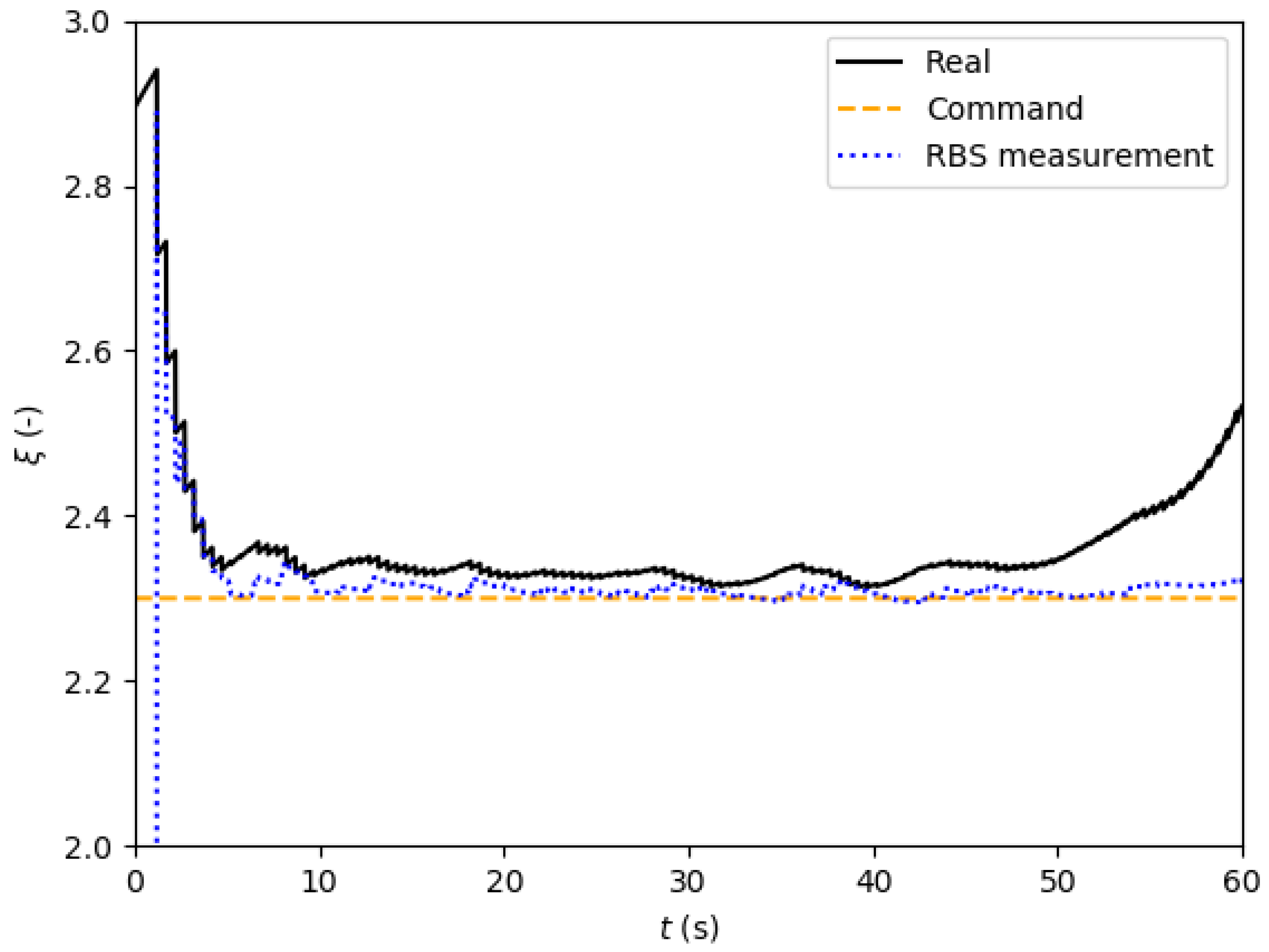
Figure 18.
Mixture ratio profile, feedback with complete regulation law, case 1.
Figure 18.
Mixture ratio profile, feedback with complete regulation law, case 1.
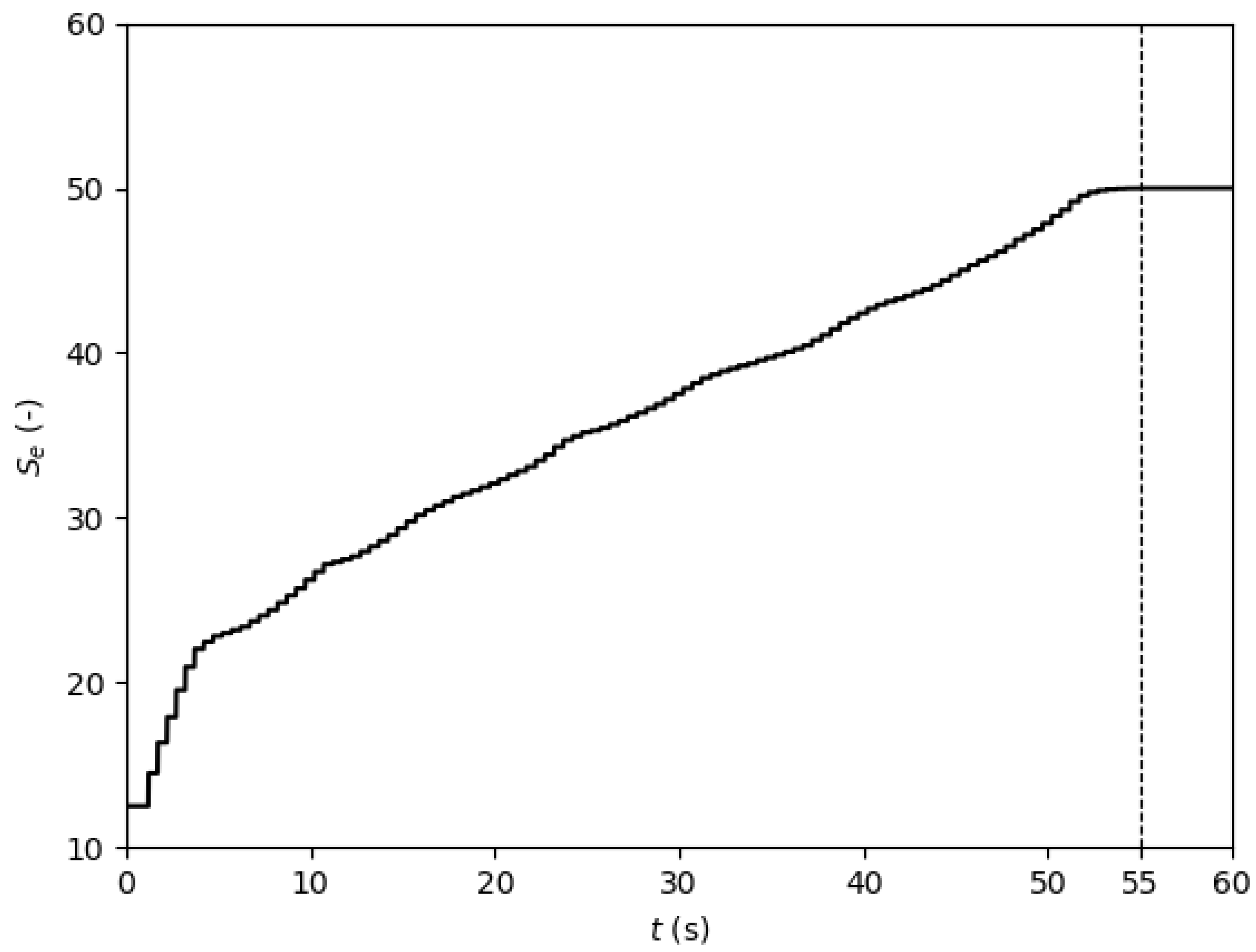
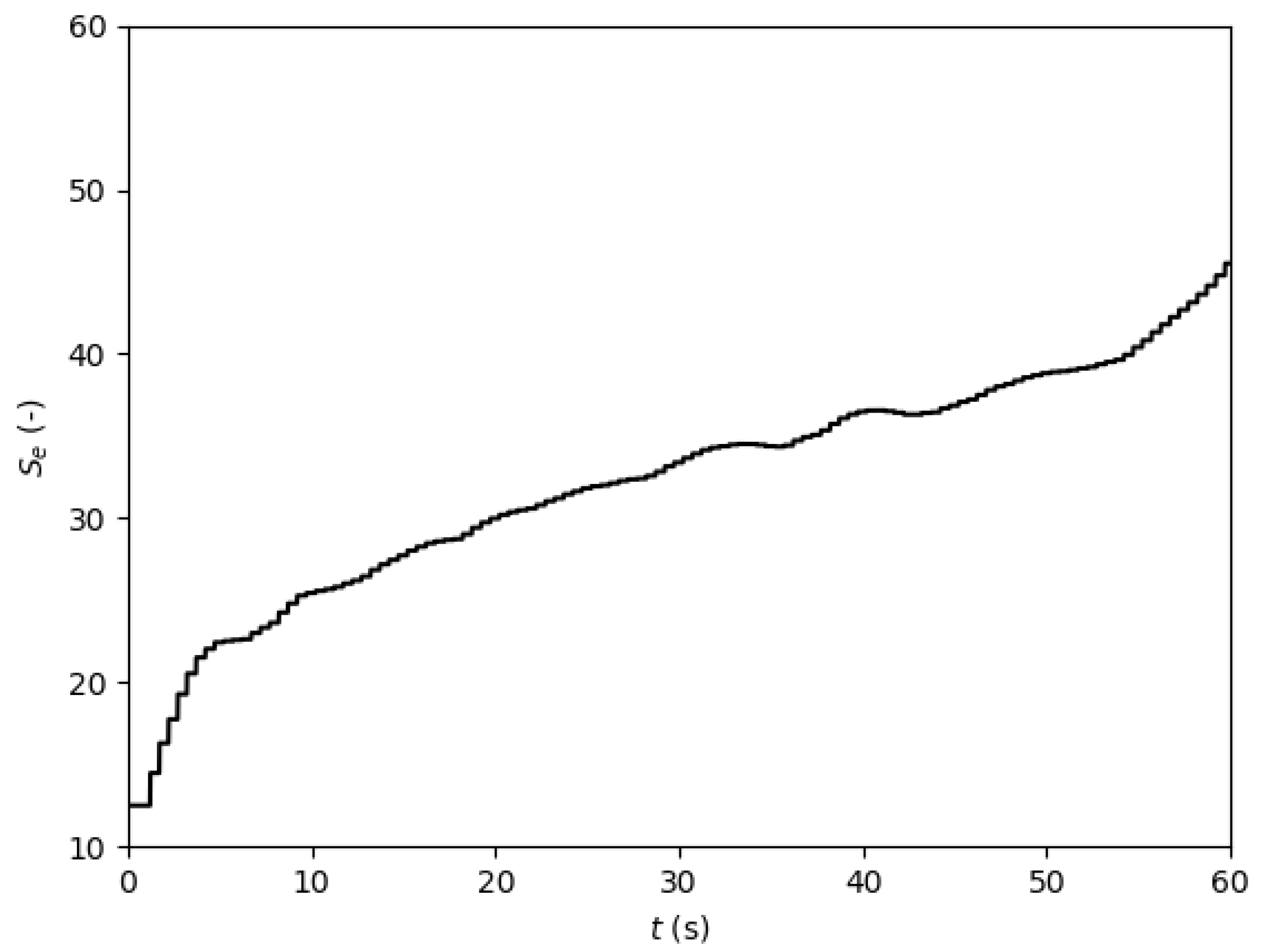
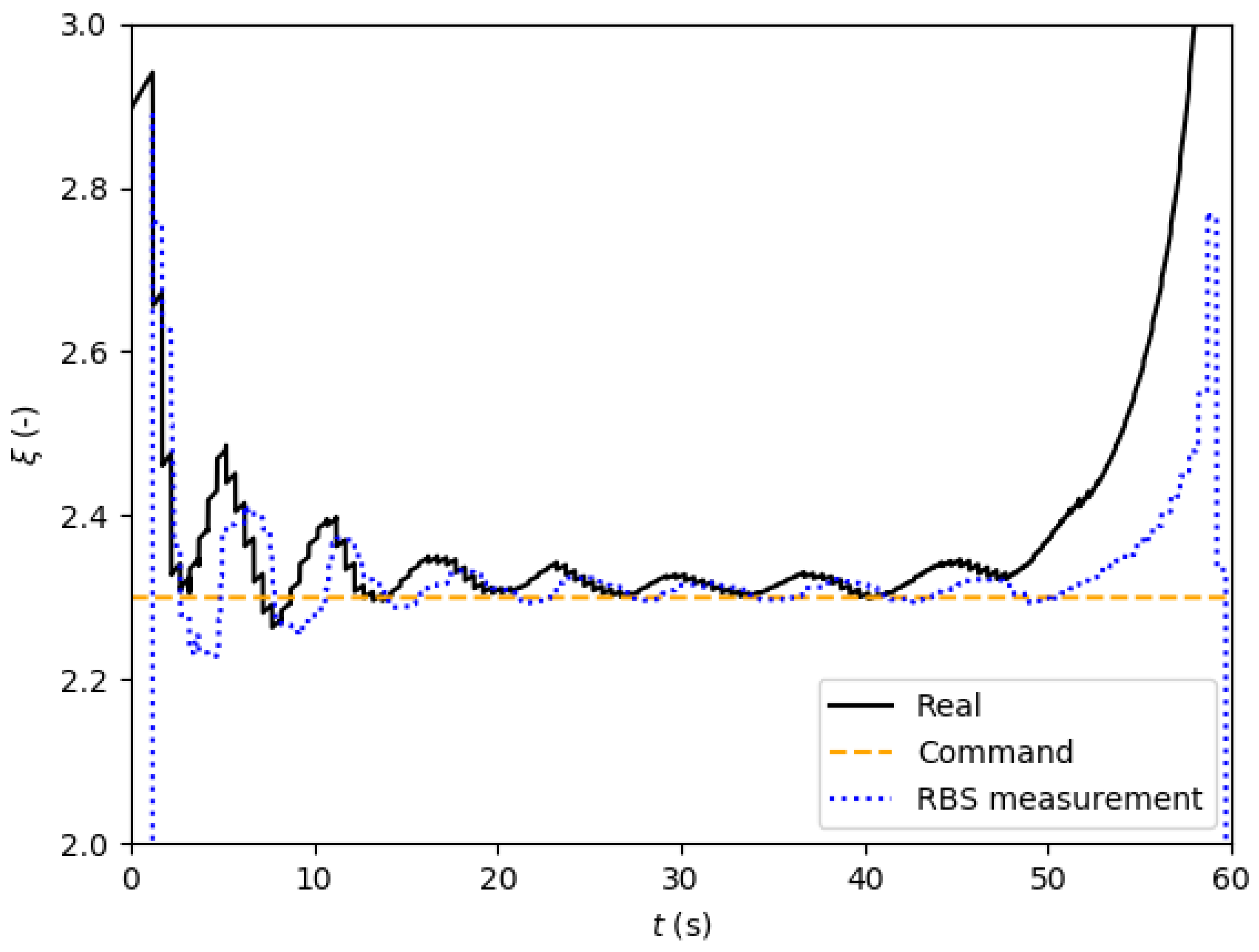
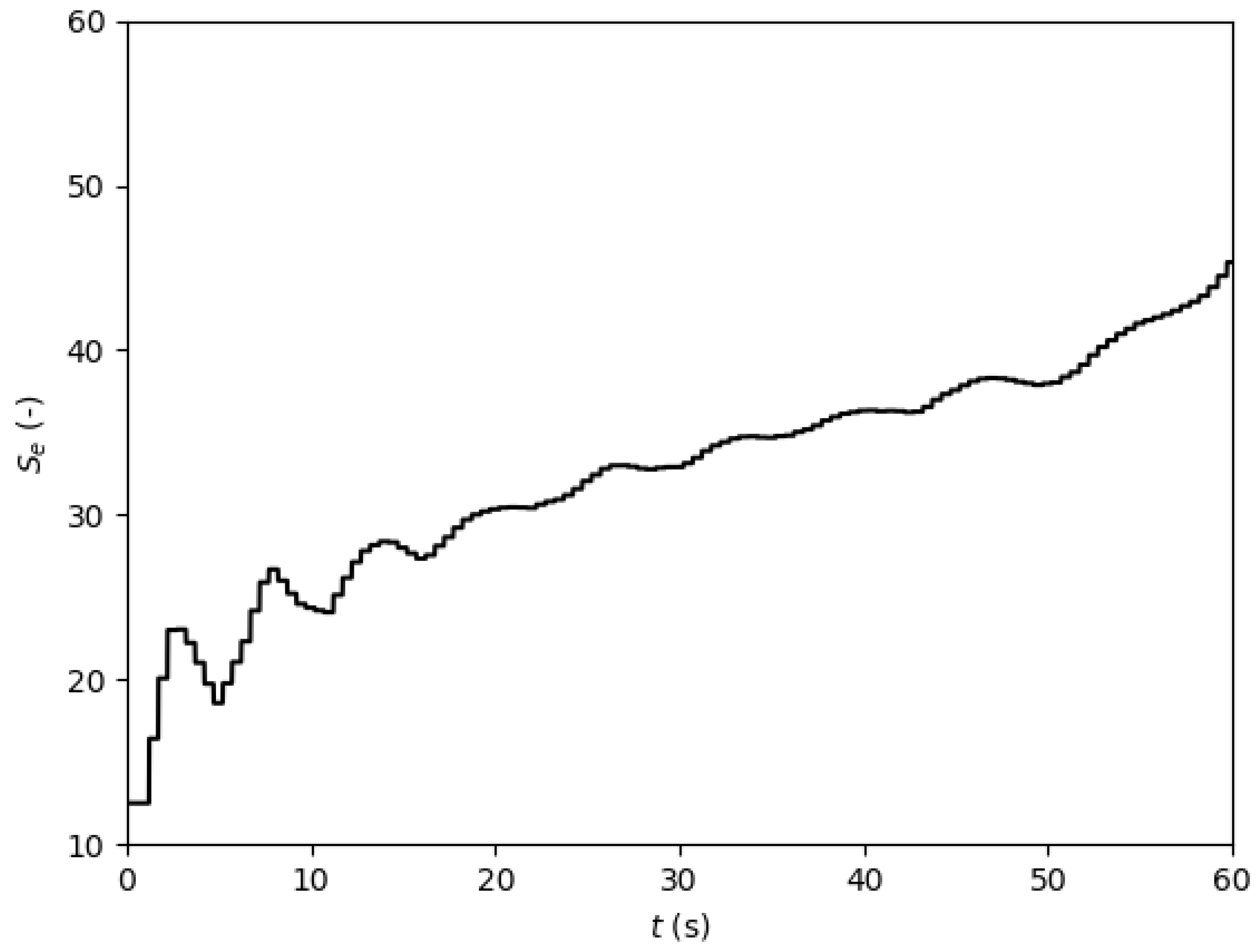
Figure 19.
Effective swirl number profile, feedback with complete regulation law, case 1.
Figure 19.
Effective swirl number profile, feedback with complete regulation law, case 1.
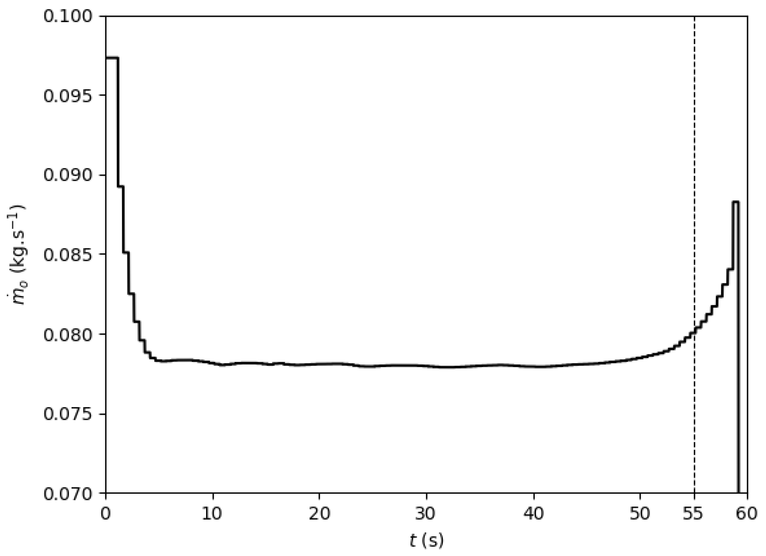
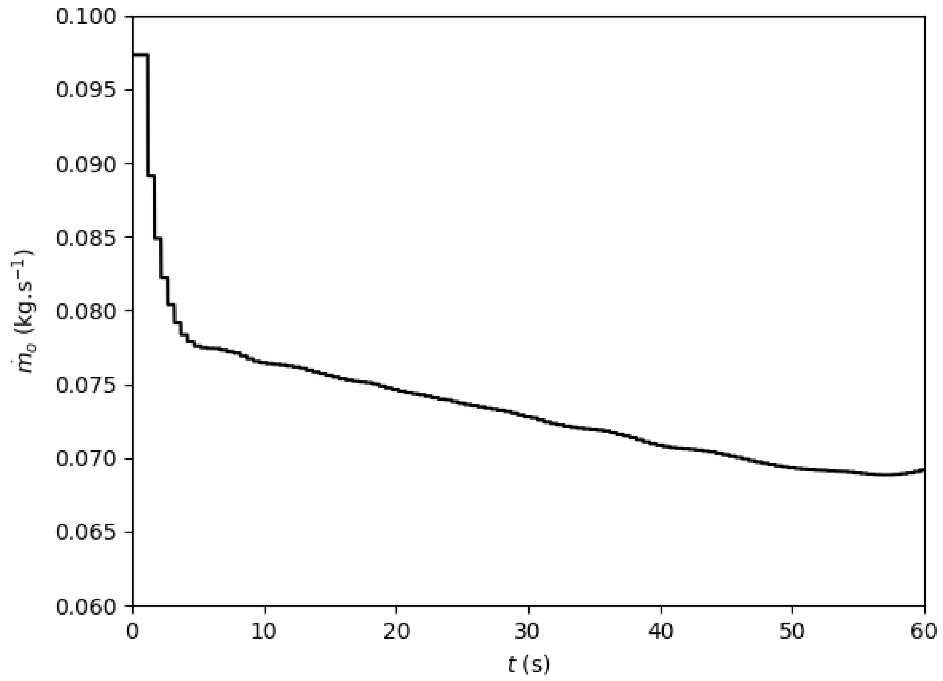
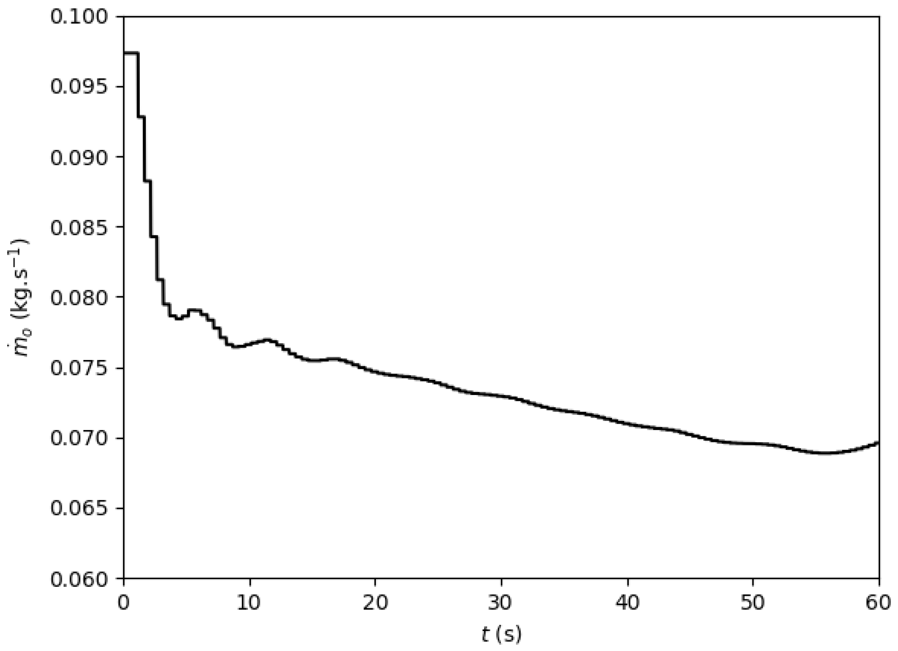
Figure 20.
Oxidizer mass flow rate profile, feedback with complete regulation law, case 1.
Figure 20.
Oxidizer mass flow rate profile, feedback with complete regulation law, case 1.
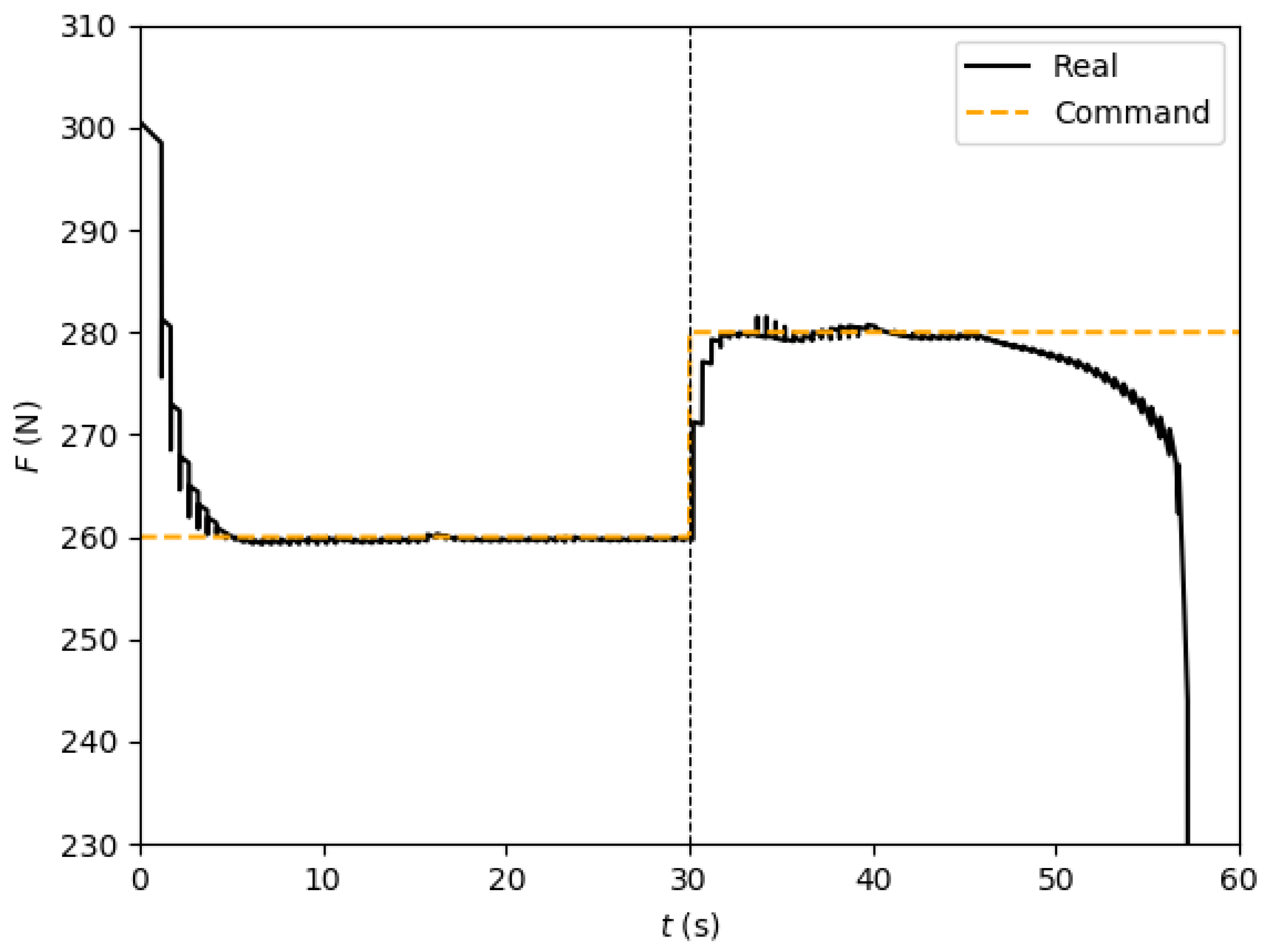
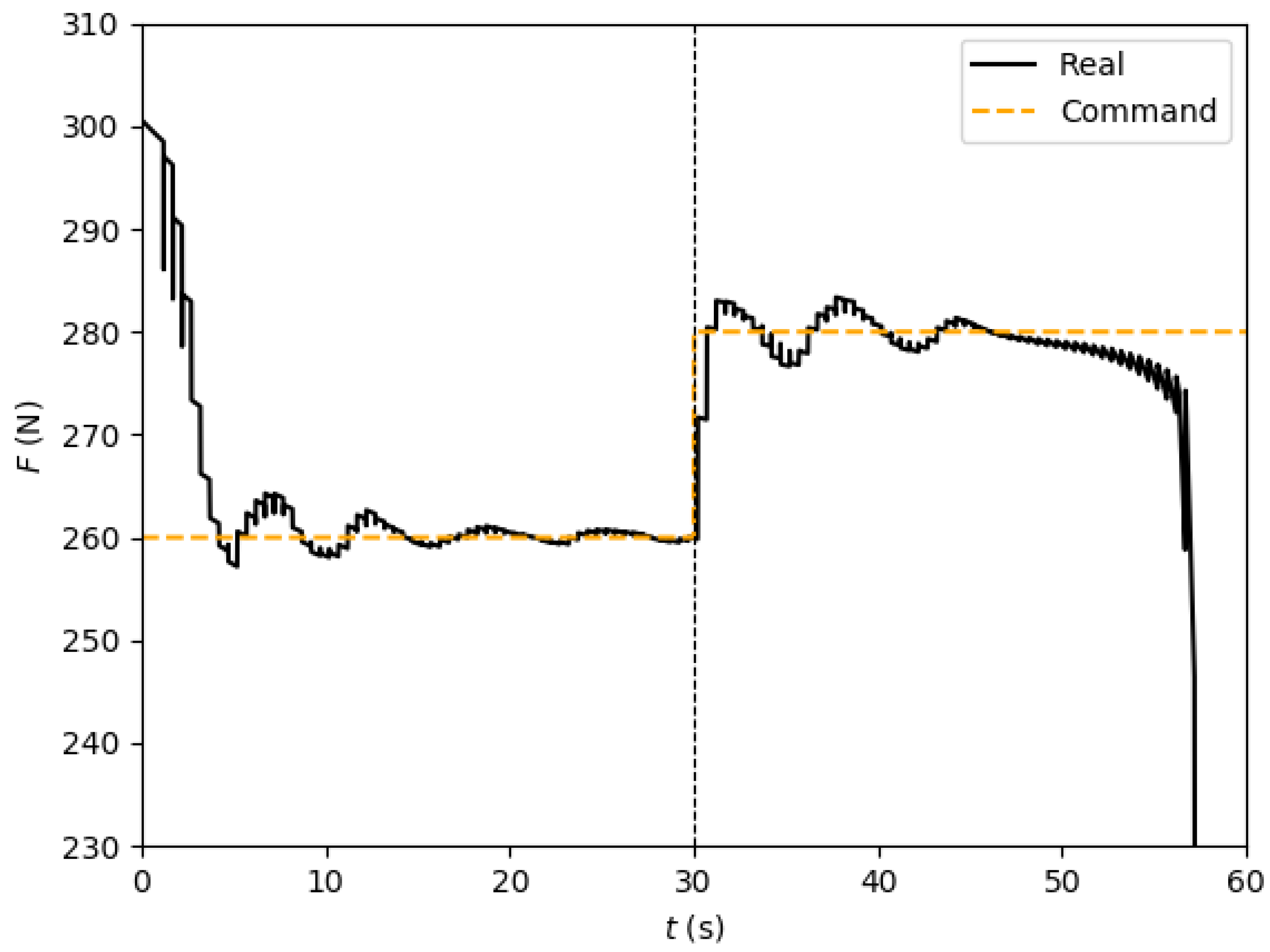
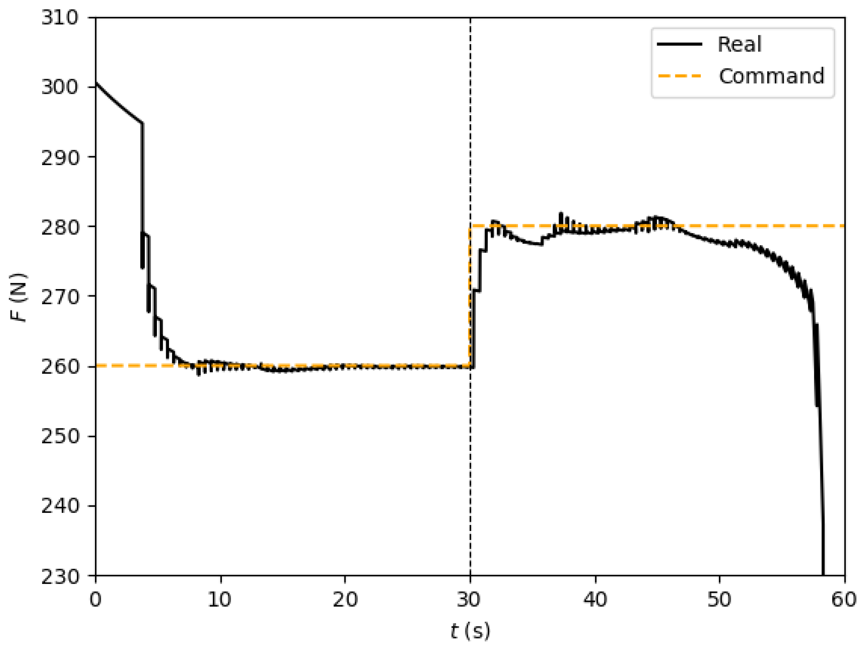
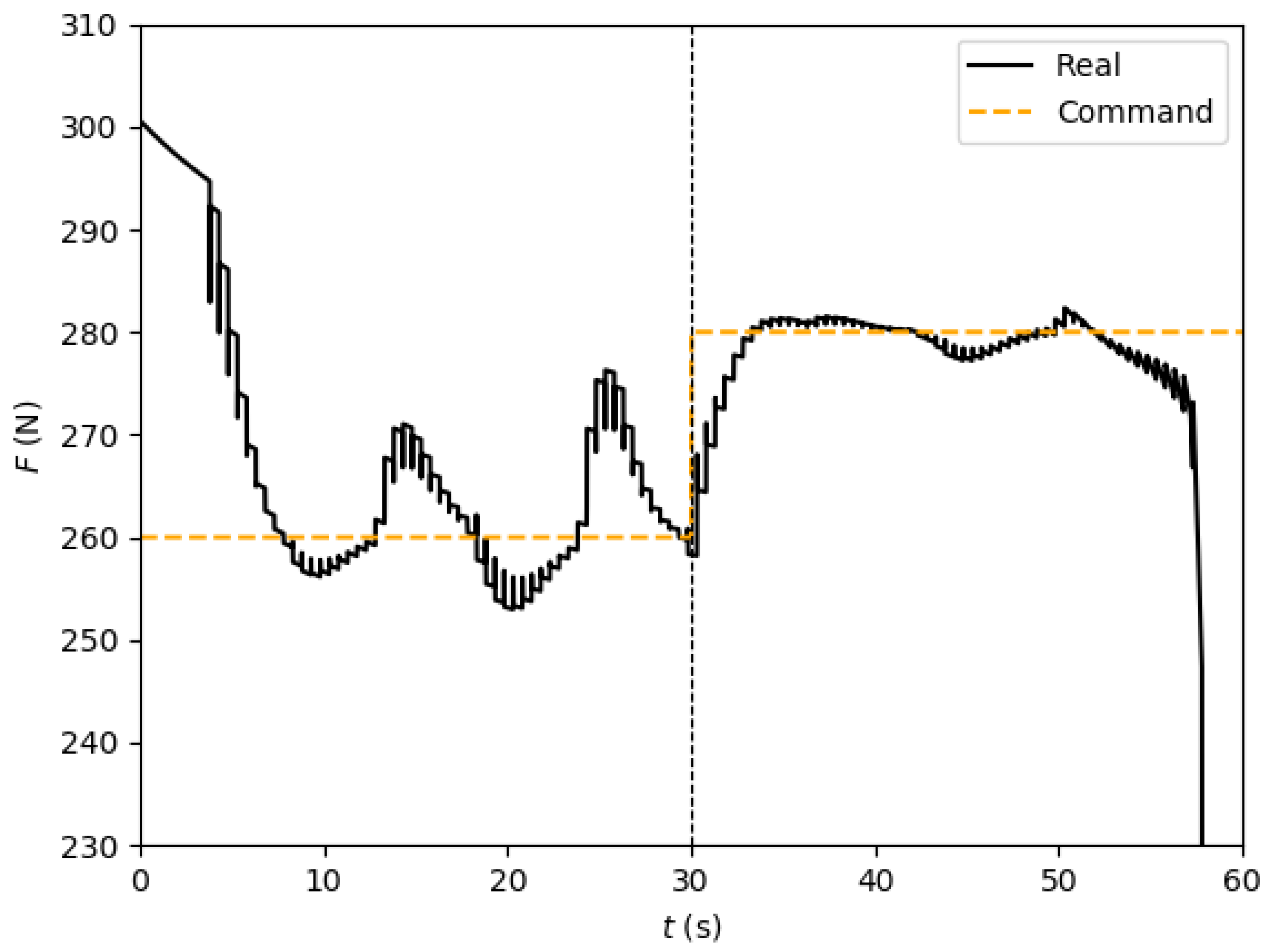
Figure 21.
Thrust profile, feedback with complete regulation law, case 2.
Figure 21.
Thrust profile, feedback with complete regulation law, case 2.
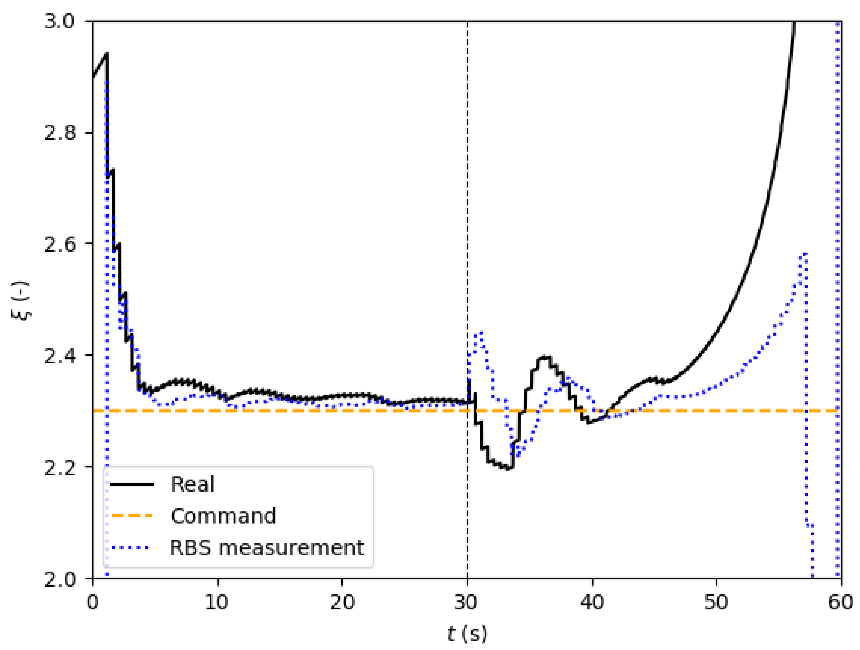
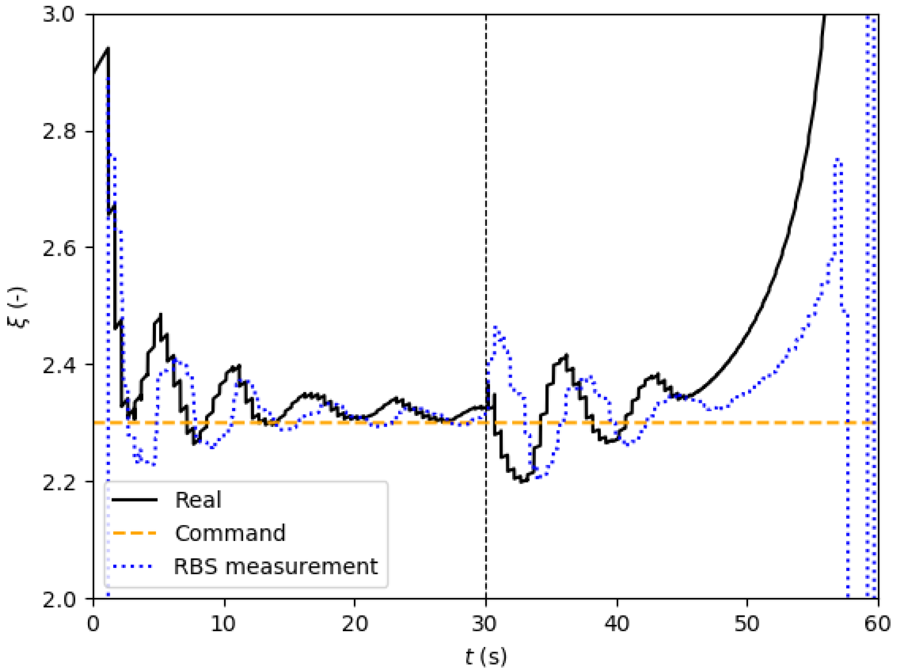
Figure 22.
Mixture ratio profile, feedback with complete regulation law, case 2.
Figure 22.
Mixture ratio profile, feedback with complete regulation law, case 2.
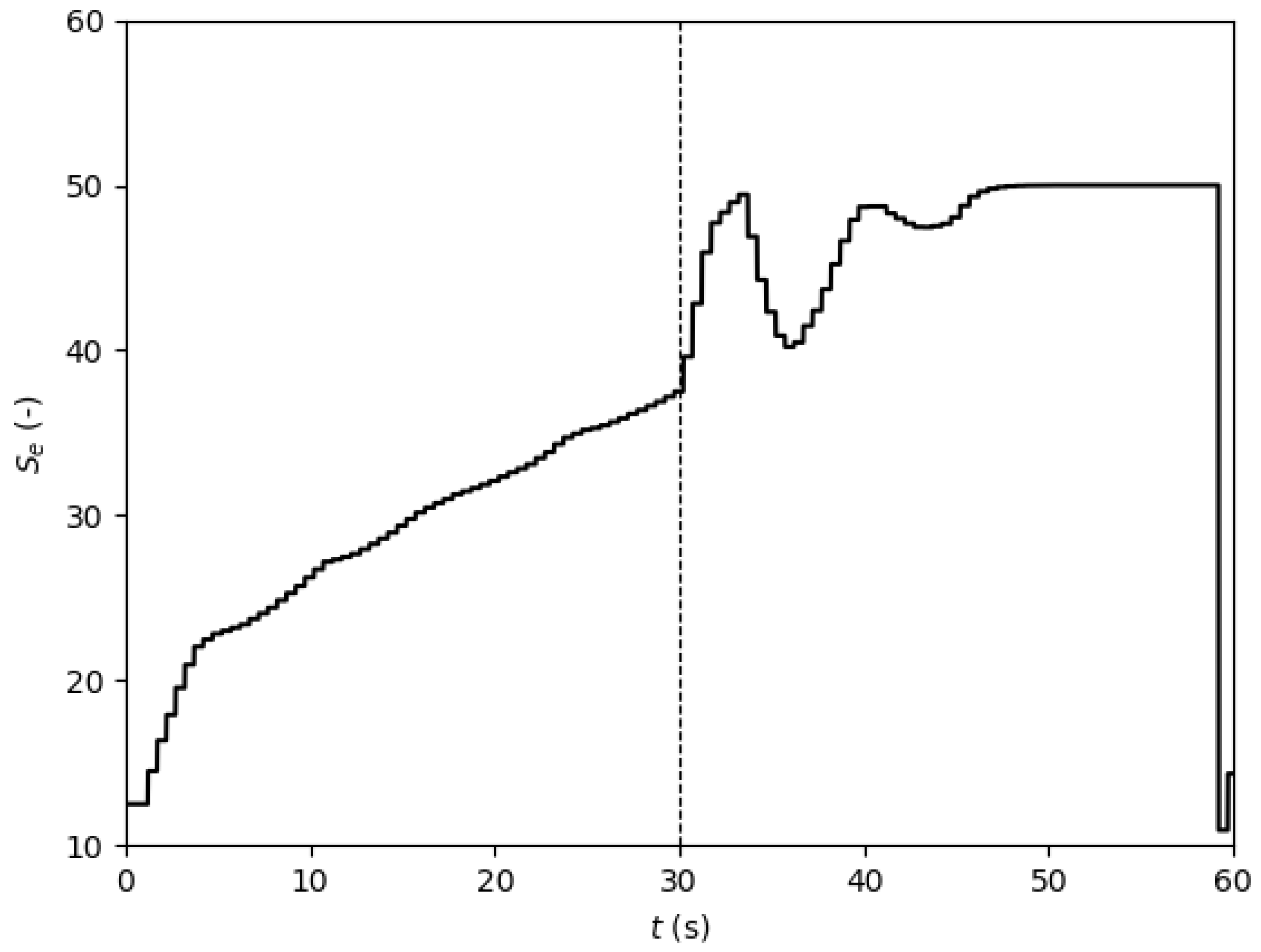
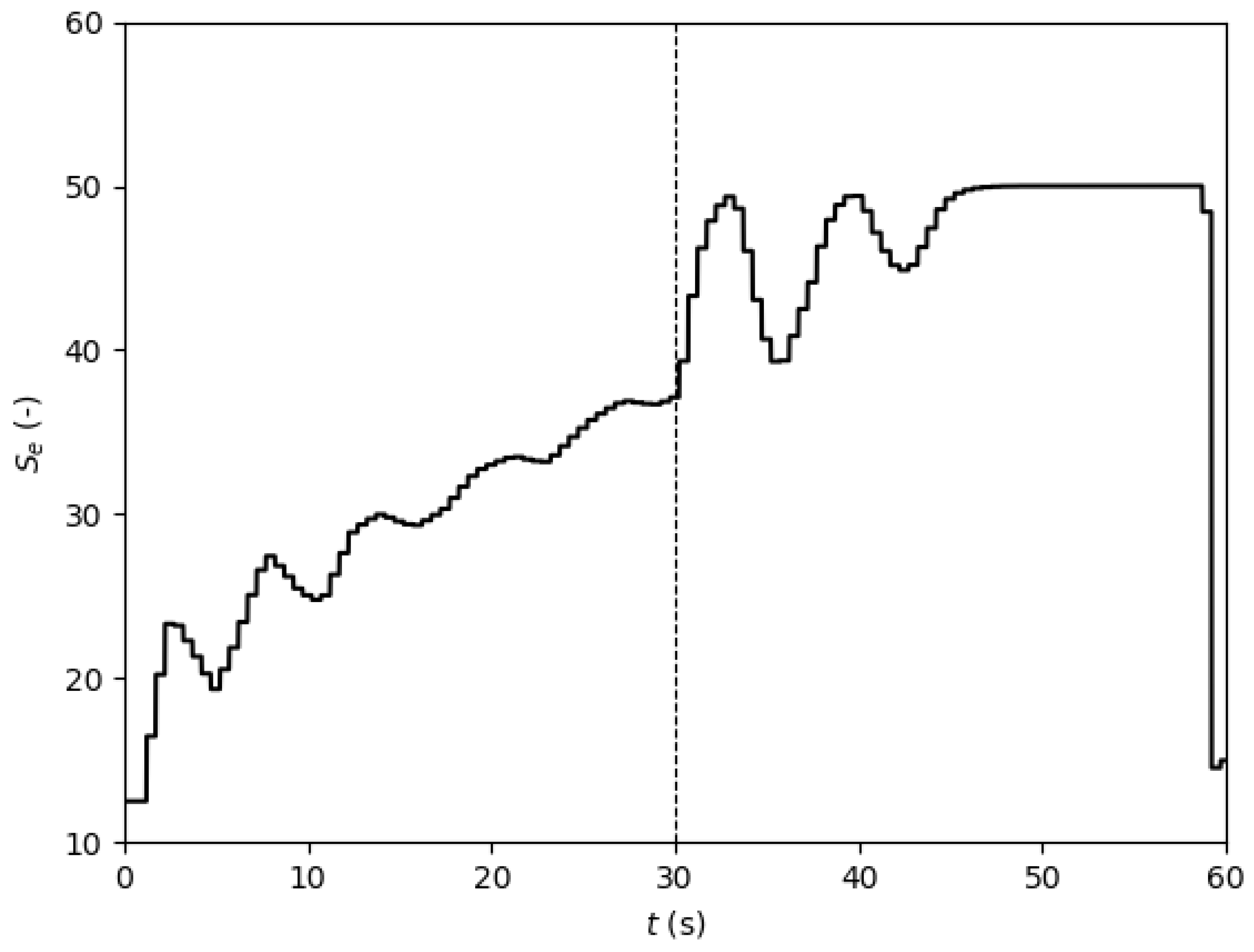
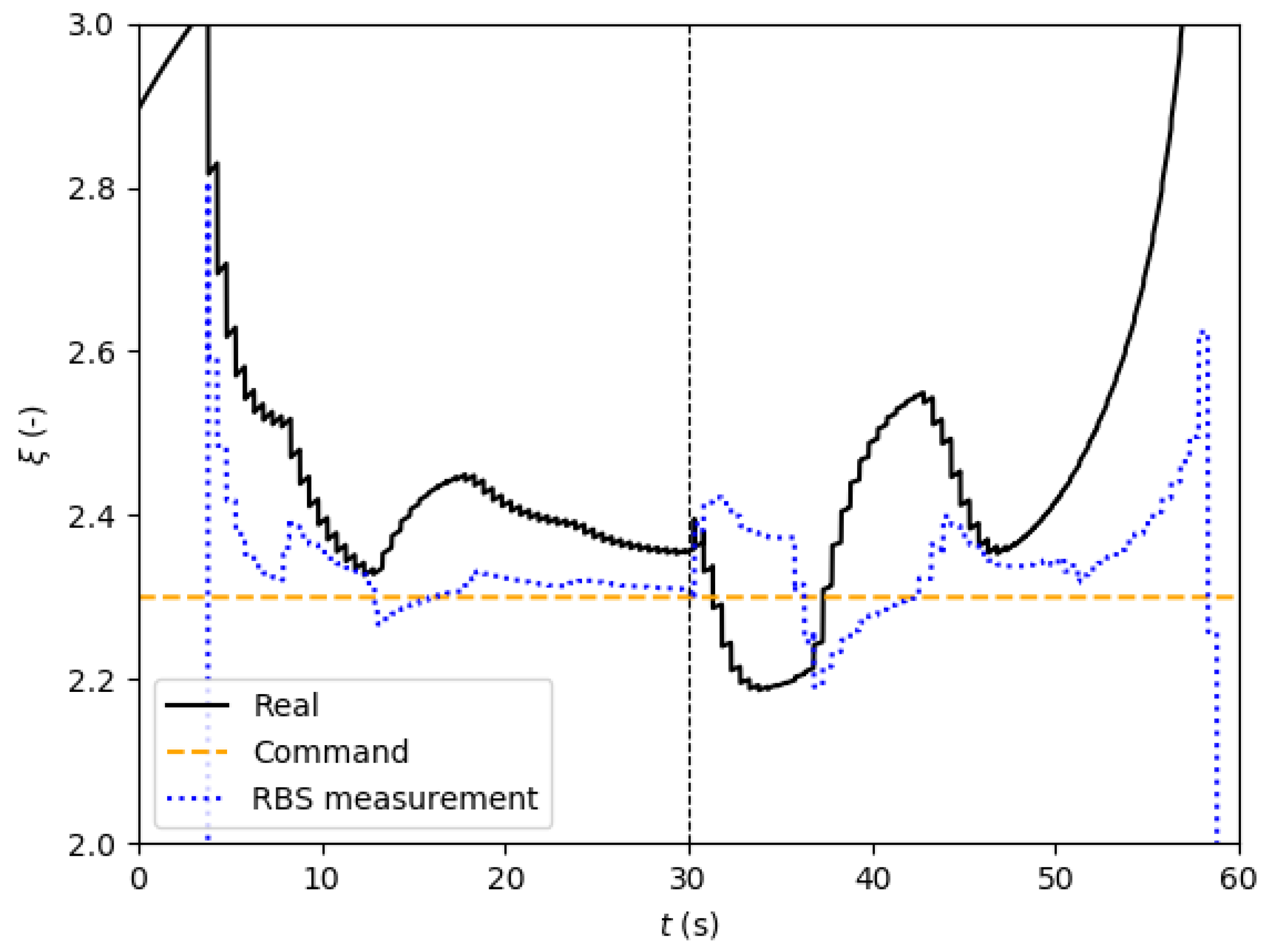
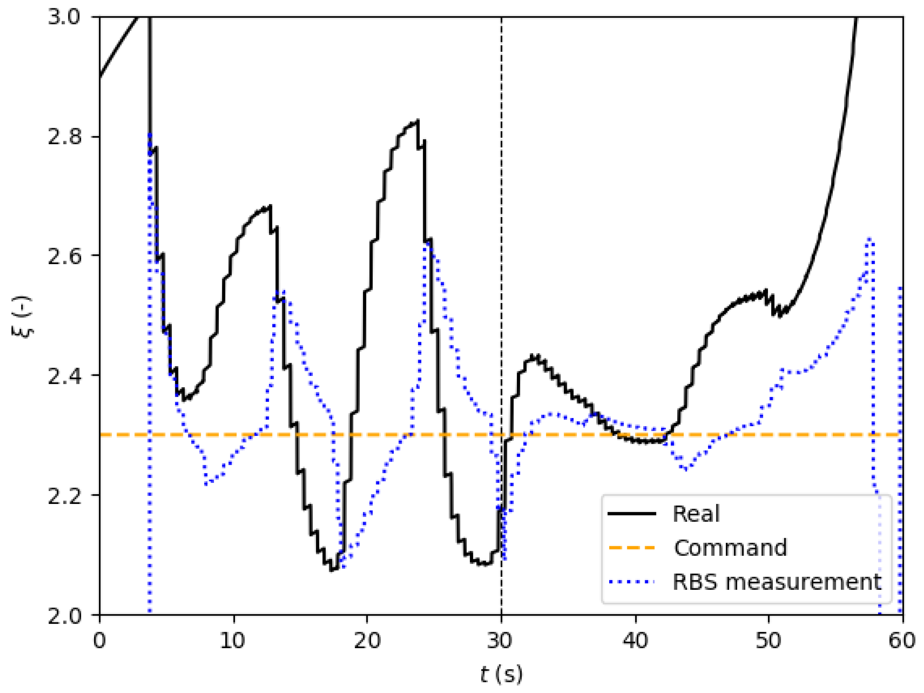
Figure 23.
Effective swirl number profile, feedback with complete regulation law, case 2.
Figure 23.
Effective swirl number profile, feedback with complete regulation law, case 2.
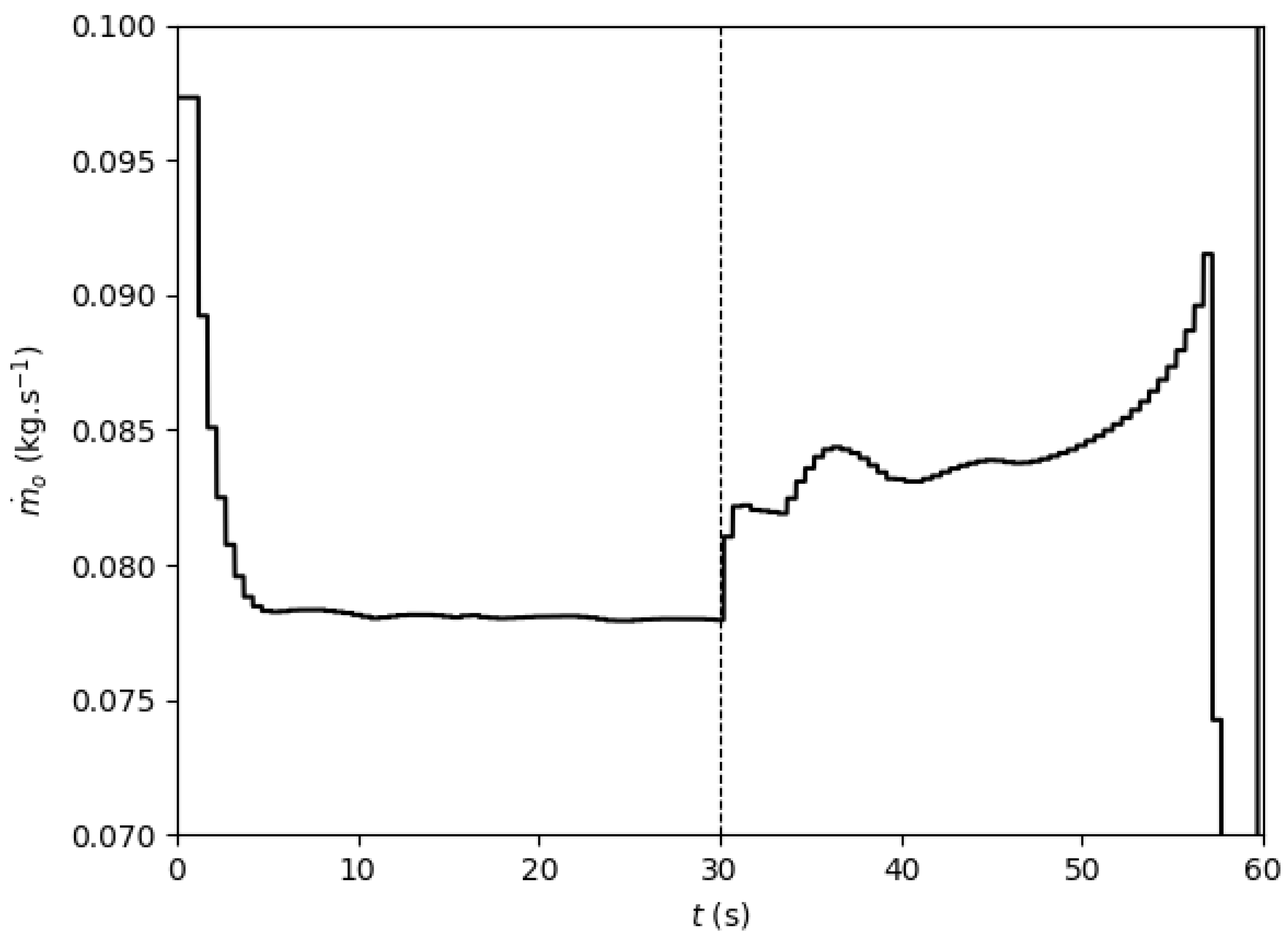
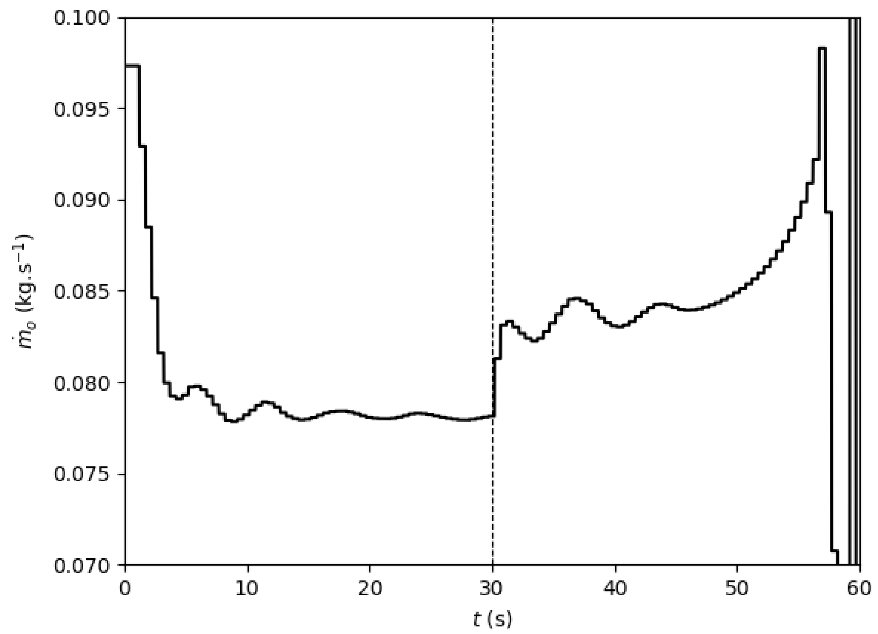
Figure 24.
Oxidizer mass flow rate profile, feedback with complete regulation law, case 2.
Figure 24.
Oxidizer mass flow rate profile, feedback with complete regulation law, case 2.
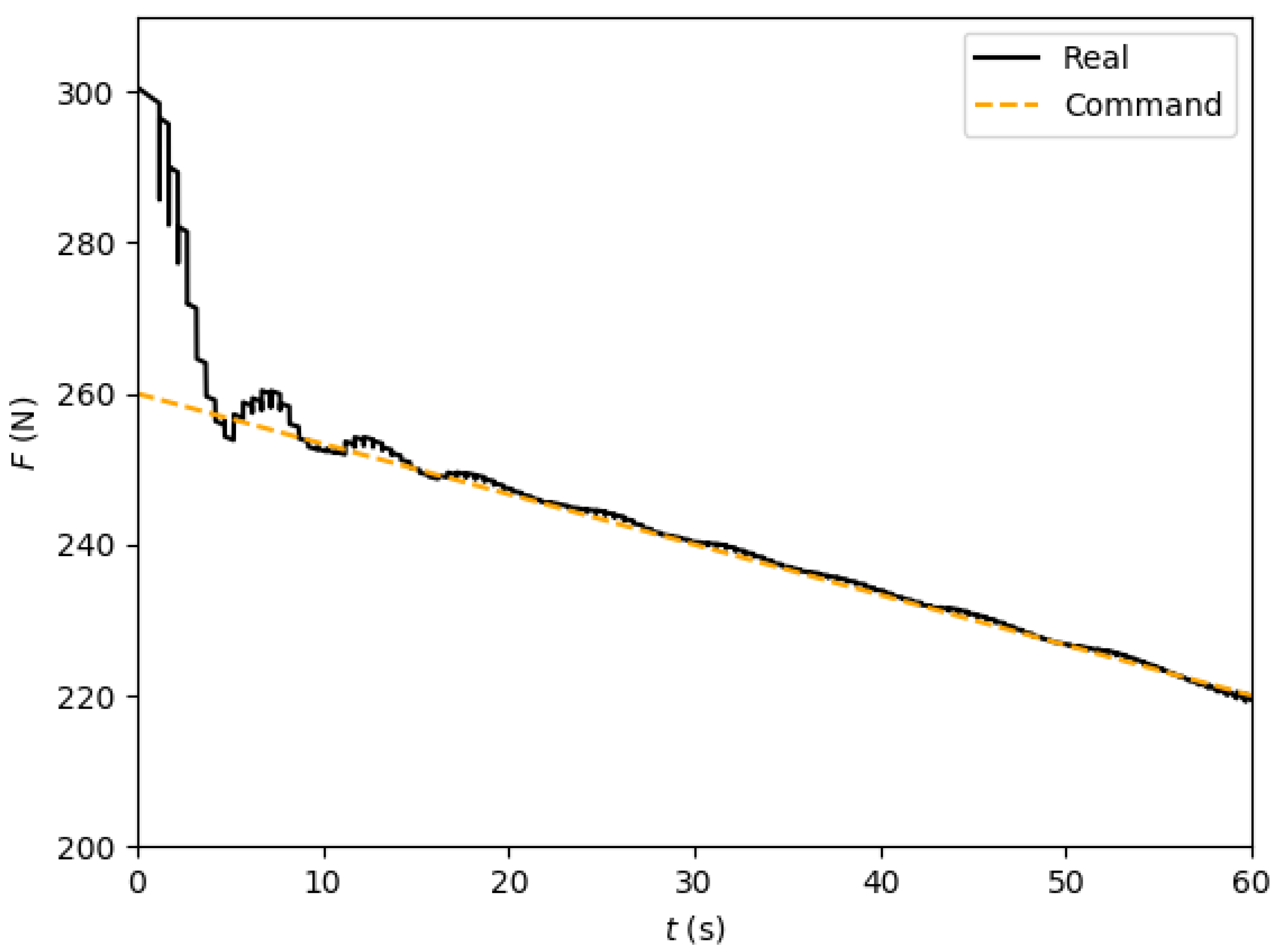
Figure 25.
Thrust profile, feedback with downgraded regulation law, case 2.
Figure 25.
Thrust profile, feedback with downgraded regulation law, case 2.
Figure 26.
Mixture ratio profile, feedback with downgraded regulation law, case 2.
Figure 26.
Mixture ratio profile, feedback with downgraded regulation law, case 2.
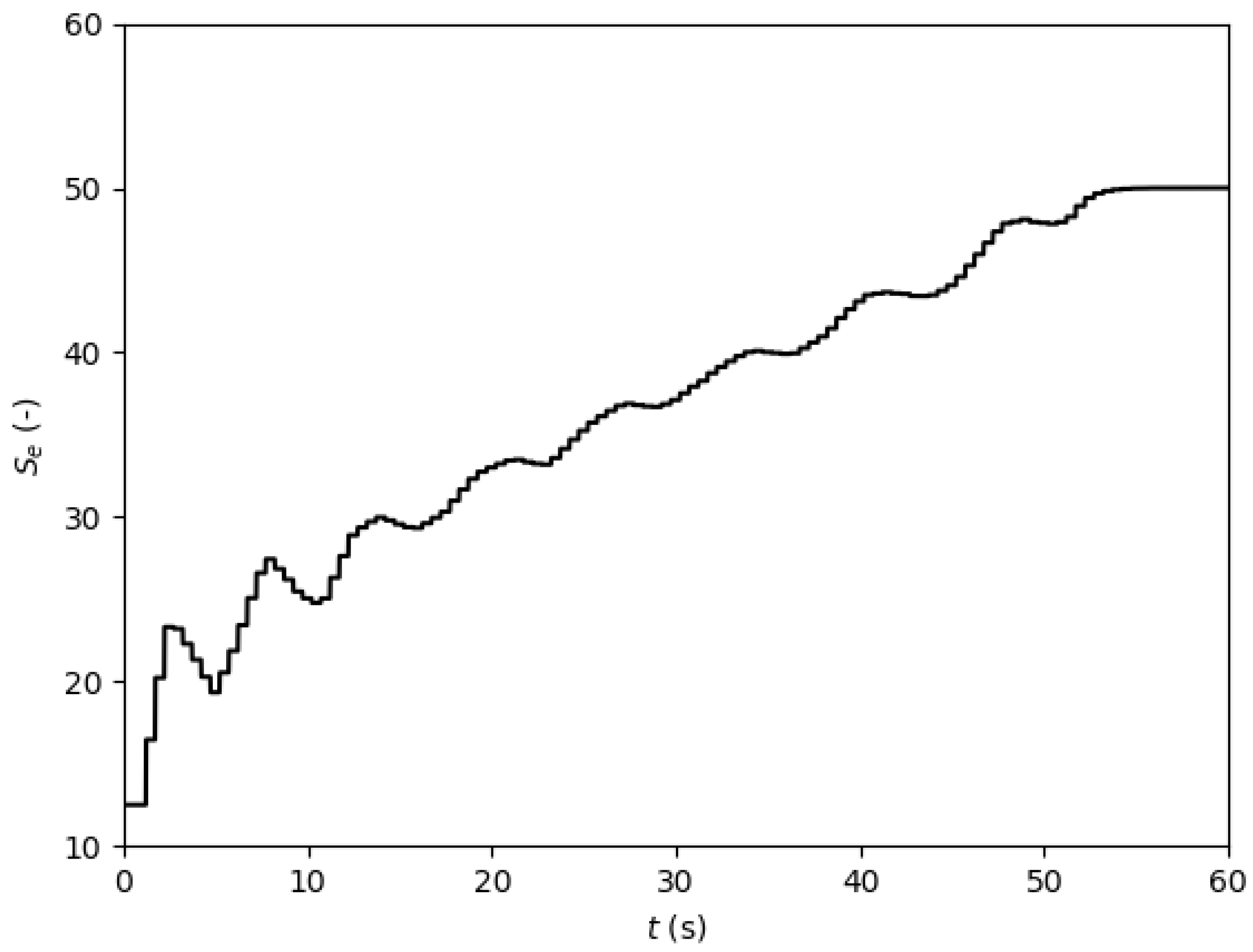
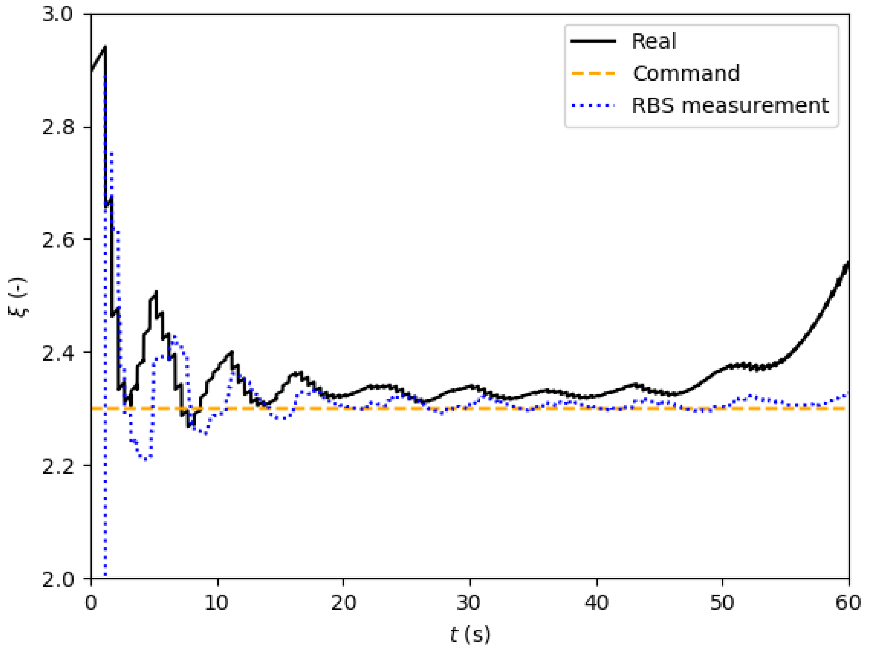
Figure 27.
Effective swirl number profile, feedback with downgraded regulation law, case 2.
Figure 27.
Effective swirl number profile, feedback with downgraded regulation law, case 2.
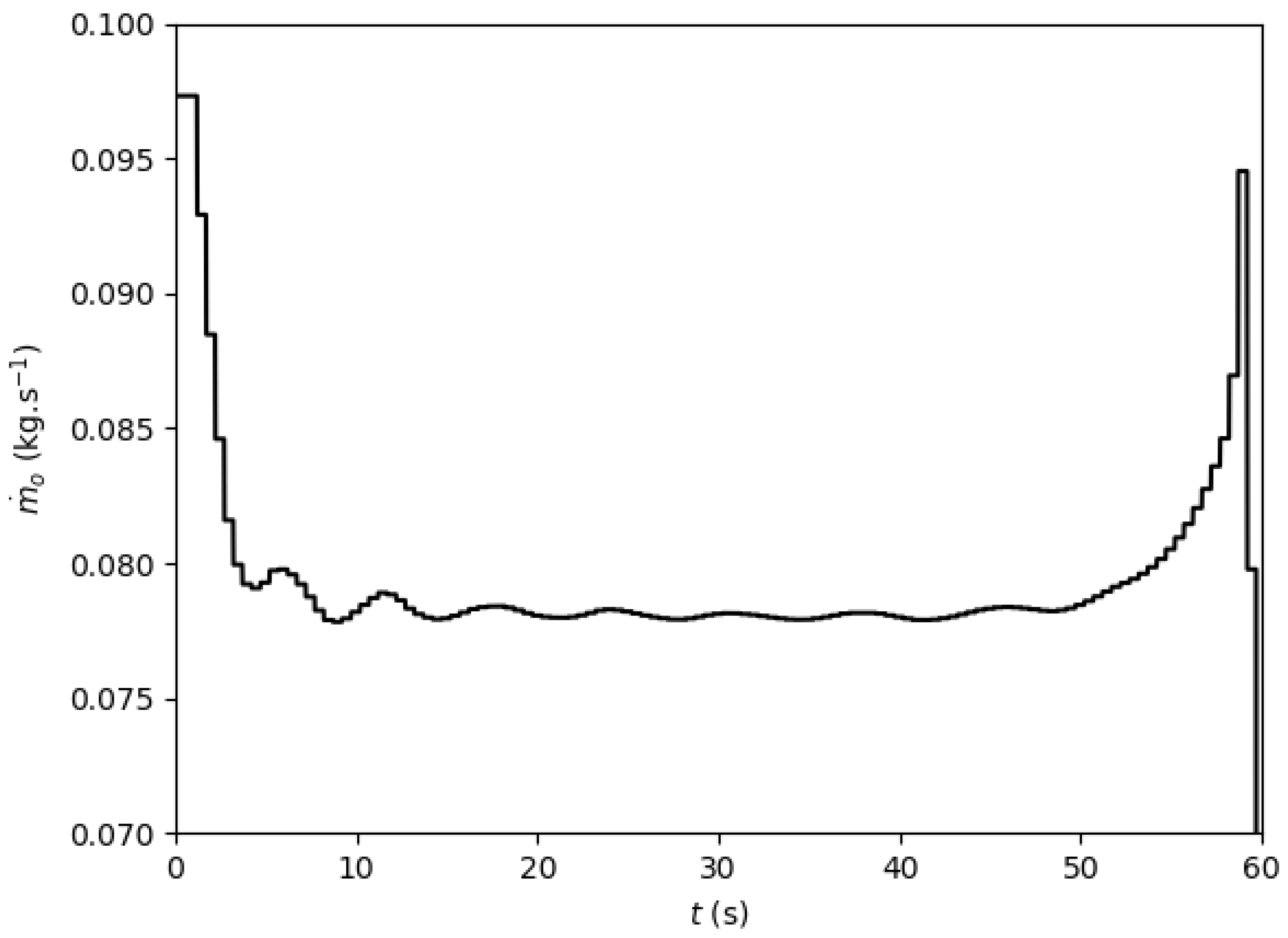
Figure 28.
Oxidizer mass flow rate profile, feedback with downgraded regulation law, case 2.
Figure 28.
Oxidizer mass flow rate profile, feedback with downgraded regulation law, case 2.
Figure 29.
Thrust profile, feedback with complete regulation law, case 3.
Figure 29.
Thrust profile, feedback with complete regulation law, case 3.
Figure 30.
Mixture ratio profile, feedback with complete regulation law, case 3.
Figure 30.
Mixture ratio profile, feedback with complete regulation law, case 3.
Figure 31.
Effective swirl number profile, feedback with complete regulation law, case 3.
Figure 31.
Effective swirl number profile, feedback with complete regulation law, case 3.
Figure 32.
Oxidizer mass flow rate profile, feedback with complete regulation law, case 3.
Figure 32.
Oxidizer mass flow rate profile, feedback with complete regulation law, case 3.
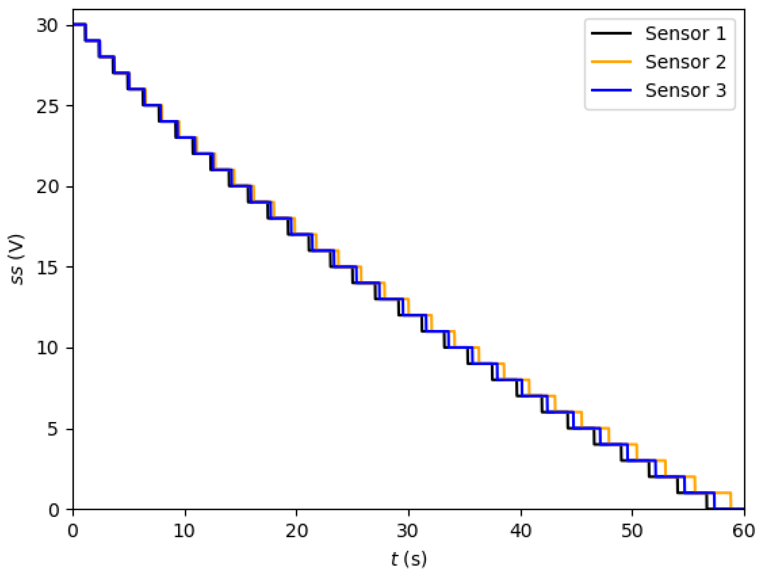
Figure 33.
RBS signals, feedback with complete regulation law, case 2.
Figure 33.
RBS signals, feedback with complete regulation law, case 2.
Figure 34.
Thrust profile, feedback with complete regulation law, case 2, mm.
Figure 34.
Thrust profile, feedback with complete regulation law, case 2, mm.
Figure 35.
Mixture ratio profile, feedback with complete regulation law, case 2, mm.
Figure 35.
Mixture ratio profile, feedback with complete regulation law, case 2, mm.
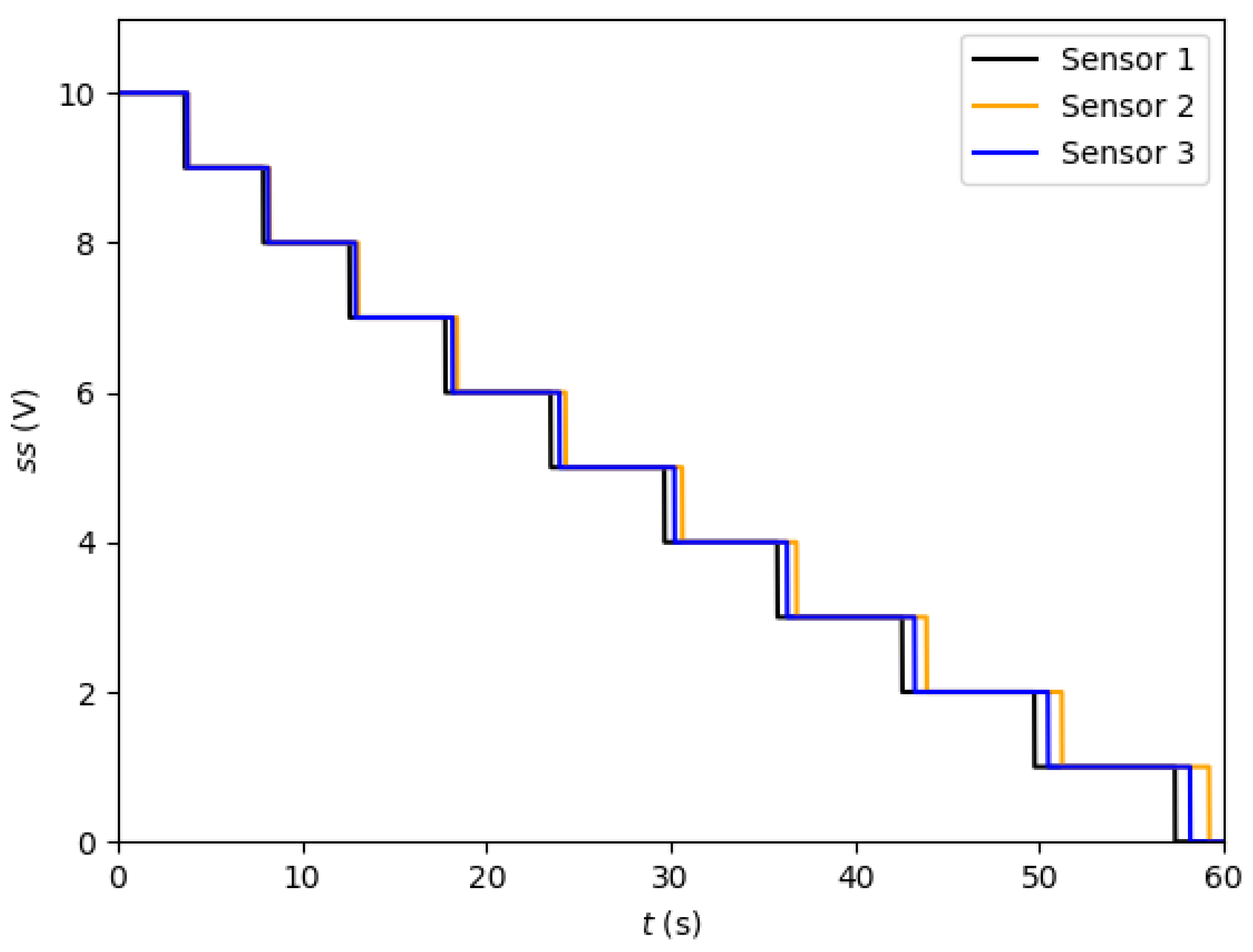
Figure 36.
RBS signal, feedback with complete regulation law, case 2, mm.
Figure 36.
RBS signal, feedback with complete regulation law, case 2, mm.
Figure 37.
Thrust profile, feedback with downgraded regulation law, case 2, mm.
Figure 37.
Thrust profile, feedback with downgraded regulation law, case 2, mm.
Figure 38.
Mixture ratio profile, feedback with downgraded regulation law, case 2, mm.
Figure 38.
Mixture ratio profile, feedback with downgraded regulation law, case 2, mm.
Table 1.
Valves’ parameters used in this study.
Table 1.
Valves’ parameters used in this study.
| (kg·s) | (-) | (-) |
|---|
| 0.1 | 0.2 | 0.15 |
Table 2.
Numerical parameters used for the simulations.
Table 2.
Numerical parameters used for the simulations.
| (m) | (s) | (%) | (Hz) |
|---|
| 0.0001 | 0.01 | 0.1 | 2.0 |
Table 3.
Examples of possible geometric swirl number and combinations for a given effective swirl number range.
Table 3.
Examples of possible geometric swirl number and combinations for a given effective swirl number range.
| Range (-) | (-) | Range (-) |
|---|
| 10–50 | 50 | 0.44–1.00 |
| 10–50 | 60 | 0.41–0.91 |
| 10–50 | 70 | 0.38–0.85 |
| 10–50 | 80 | 0.35–0.79 |
Table 4.
Numerical simulations’ parameters.
Table 4.
Numerical simulations’ parameters.
| L (m) | (m) | (m) |
| 0.330 | 0.040 | 0.100 |
| (s) | (Pa) | (m·s) |
| 60.0 | 0.1 × 10 | 9.81 |
| (m) | (-) | (-) |
| 0.010 | 3.0 | 50.0 |
| (kg·m) | (-) | (m·s) |
| 905.0 | 0.9 | 2.0 × 10 |
| (-) | (-) | (-) |
| 0.1392 | 0.64 | −0.10 |
| (-) | (-) | (-) |
| 0.30 | 0.30 | 2.3 |
| (kg·s) | (kg·s) | (-) |
| 0.049 | 0.049 | 0.5 |
Table 5.
RBS (Resistor-Based Sensors) parameters for the simulations.
Table 5.
RBS (Resistor-Based Sensors) parameters for the simulations.
| (m) | (m) | (-) | (-) |
|---|
| 0.001 | 0.001 | 30 | 3 |
Table 6.
PID (Proportional Integral Derivative) parameters for the simulations.
Table 6.
PID (Proportional Integral Derivative) parameters for the simulations.
| (-) | (-) | (-) |
|---|
| 0.45 | 0.0 | 0.0 |
Table 7.
New RBS parameters for the simulations.
Table 7.
New RBS parameters for the simulations.
| (m) | (m) | (-) | (-) |
|---|
| 0.003 | 0.003 | 10 | 3 |


