Identification of In-Flight Wingtip Folding Effects on the Roll Characteristics of a Flexible Aircraft

Abstract

Wingtip folding is a means by which an aircraft’s wingspan can be extended, allowing designers to take advantage of the associated reduction in induced drag. This type of device can provide other benefits if used in flight, such as flight control and load alleviation. In this paper, the authors present a method to develop reduced order flight dynamic models for in-flight wingtip folding, which are suitable for implementation in real-time pilot-in-the-loop simulations. Aspects such as the impact of wingtip size and folding angle on aircraft roll dynamics are investigated along with failure scenarios using a time domain aeroservoelastic framework and an established system identification method. The process discussed in this paper helps remove the need for direct connection of complex physics based models to engineering flight simulators and the need for tedious programming of large look-up-tables in simulators. Instead, it has been shown that a generic polynomial model for roll aeroderivatives can be used in small roll perturbation conditions to simulate the roll characteristics of an aerodynamic derivative based large transport aircraft equipped with varying fold hinge lines and tip deflections. Moreover, the effects of wing flexibility are also considered.

1. Introduction

In the scope of a wider research project led at Cranfield University, the aim of this work was to quantify the impact of a specific in-flight dihedral folding wingtips system on the lateral flight dynamics of a large generic civil aircraft. With aircraft handling qualities and pilot-in-the-loop simulations in mind, this work focused on capturing roll damping and aileron effectiveness changes with wingtip angle, quantities widely used by pilots for roll performance and lateral handling qualities analysis. Figure 1 illustrates the logical link between the various elements of this research, from test case definition, tool and method presentation, aerodynamic derivative identification and prediction model derivation.

The motivation behind this interest for in-flight folding wingtips is presented in the  Introduction. Section 2 is dedicated to the kinematic and geometric description of the flared folding mechanism used herein and past publications [1,2,3]. The device was implemented within the Cranfield Accelerated Aeroplane Loads Model (CA${}^2$LM), briefly presented in Section 3. This non-linear six degrees of freedom aircraft flight simulation environment was used to compute flight dynamic responses of a morphing aircraft in various folding and flight conditions based on a physics based model of the folding wingtip system. A conventional systems identification method, described in Section 4, was then used to quantify the lateral aerodynamic derivatives of interest over a wide range of test cases (flight conditions and symmetric folding configurations). Thus, a more robust and widely applicable set of results can be obtained and used in real time flight simulators [4]. Results from this identification procedure are presented in Section 5. Polynomial approximations of changes due to wingtip folding, or prediction models, were also investigated and are presented in Section 6. This formulation, similar to current practices used to model flaps or undercarriages effects [5] is intended for any aerodynamic derivative based flight simulator using a comparable aircraft and not only allows the modeling of folding wingtip aerodynamic shifts without the need of extensive databases or complex models but can also be used for stability and control analysis purposes. The paper concludes with a general discussion in Section 7 regarding the impact of in-flight wingtip folding on flight dynamics and possible handling qualities concerns for certification purposes.

Ground dihedral folding was historically proven to be an efficient method to cope with limited storage and ground operational dimensions. It saw great success on naval based aircraft as early as the 1940s with the F4U Corsair, and is still used today on naval based aircraft such as the Lockheed Martin F-35C [6]. Hence, engineers have also considered this solution to reduce wingspan of large civil aircraft, implementing the now certified wingtip folding devices on the Boeing 777-X and the Boeing SUGAR concept [7]. If fitted with a wingtip dihedral folding device, the HARW concepts could qualify in comparable aircraft size categories and, therefore, be operated within the same infrastructures as their predecessors. This would avoid additional operational costs to airports and airlines, which could potentially prevent such a design to ever be brought to market. On the other hand, the implementation of this mechanism brings additional costs in design, maintenance, operational complexity and aircraft flight efficiency.

Using the classic Breguet range equation, one can focus purely on aircraft flight efficiency. It is easy to comprehend that the addition of the folding device mass (and subsequent structural changes required to accommodate it) will greatly reduce aircraft performances [8], jeopardizing initial design objectives. Therefore, the identification of a number of in-flight folding benefits would greatly aid and justify the development and implementation of folding wingtips. The benefits of folding wingtips for loads alleviation has already been demonstrated for large commercial aircraft [2,3] with multiple actuation strategies for such devices. A sub-scaled demonstrator was also flown recently as part of the Spanwise Adaptive Wing (SAW) project [9]. The NASA led tests highlighted the potential for subsonic commercial applications of in-flight dihedral wingtip morphing, including increased fuel-efficiency, increased controllability and possibility to reduce tail size as deflected wingtips offered enhanced directional stability. This has also been extensively discussed on the XB-70 aircraft [10,11,12]. Experimental data from wind-tunnel tests of a mini-Unmanned Aerial Vehicle (UAV) equipped with folding wingtips intended for roll control [13,14] have shown significant modifications to both lateral and directional aerodynamic derivatives as a function of flight conditions and fold angles. Additionally, it could be argued that the use of folding wingtip devices could also be used on even smaller scales such as Micro AV (MAV) designs [15] for attitude control and performance augmentation. In the latter cases of MAV and UAV (and even the XB-70), relatively low aspect ratio wings tend to benefit more from folding wingtips as control surfaces or directional stability enhancements whilst higher aspect ratio may also see benefits directly on roll performances and potential loads alleviation applications.

In any case, these past findings and examples highlight that wingtip folding does have a significant impact on aircraft flight dynamics. In other words, the response to pilot inputs or external disturbances will change with wingtip deflection. The amplitude of the shift in flight dynamic properties relative to the baseline shape must therefore be quantified and assessed for certification, pilot training or for the purpose of adequate flight control augmentation. Past work from the authors [1] presented an initial discussion regarding the impact of airframe flexibility and wingtip dihedral folding on a large civil aircraft. For a smaller set of flight conditions, significant differences in lateral aerodynamic derivatives between rigid and flexible airframe simulations were outlined. The impact of wingtip folding itself was also highlighted. These results were encouraging for certification, pilot training [4] or augmentation purposes, as the shift in the aerodynamic derivatives was relatively small with folding for a device capable of significantly reducing span for ground operations. However, further work is needed over a wider range of flight conditions and folding angles.

2. In-Flight Folding Wingtip Device Characteristics

The development and selection process of the folding wingtip device lays outside the scope of this paper. However, the requirements can be summarized as follows: (a) significantly reduce aircraft wingspan during ground operations; (b) provide aerodynamic loads alleviation capability, both through controlled and soft failed (released) actuation; and (c) rely on conventional actuators for wing folding (hydraulic or electric motors). As a result of prior studies, a hybrid twist-dihedral folding system was adopted. Using a flared hinge line angle, the dihedral rotation of the wingtip leads to an effective twist modification [2]. Thus, aerodynamic loads alleviation is achieved by reducing the angle of attack or local twist of the aerofoil as wingtip is folded. A sketch of the device geometry is given in Figure 2a, where the hinge line is rotated around the vertical axis by a non-zero flare angle ${\Lambda }_{hinge}$ shown in dark red. Hence, dihedral rotation leads to an effective twist angle modification, given by:

$$\Delta {\theta }_{wt}={tan}^{-1}\left(tan\left({\Lambda }_{hinge}\right)\times sin\left({\Gamma }_{wt}\right)\right)$$

(1)

where $\Delta {\theta }_{wt}$ is the change in local twist angle due to the dihedral fold angle ${\Gamma }_{wt}$ and hinge flare angle ${\Lambda }_{hinge}$ as defined in Figure 2a. A geometrical derivation of Equation (1) is given Appendix A. A hinge line pointing outward on the leading edge effectively leads to a decrease in local angle of attack for an upward dihedral rotation. Symmetrically, an inward pointing hinge line leads to an increase in angle of attack with upward folding [2]. Twist angle evolutions for different hinge flare angles are illustrated in Figure 2b, with an emphasis on the flare angle ${\Lambda }_{hinge}={17}^{\circ }$ selected for this specific investigation. Note that the aerodynamic limitations of the aeroservoelastic framework and the maximum wingtip folding angle used herein are included on the graph for illustrative purposes, showing that wingtip local angle of attack shift due to folding is kept below ${10}^{\circ }$.

The actuation dynamics of the device are also a critical aspect of the design. The actuation device, which should be effective at both unloading the wing under excessive gust or maneuver loads and restoring the wingtip after a high load incident, is not investigated here. The transient dynamics of a release or failure are also not considered at this stage of the investigation. The device is assumed to fit within the profile without the needs of an additional fairing at the hinge line.

3. Modeling the Wingtip in an Aeroservoelastic Framework

3.1. CA${}^2$LM Overview

The Cranfield Aircraft Accelerated Loads Model (CA${}^2$LM)  framework [16,17] is an aeroservoelastic simulation tool developed in MATLAB/Simulink and capable of near real-time simulations. It couples both linear structural model with unsteady aerodynamics in the time domain to couple aircraft flight dynamics with aeroelastics. Unsteady aerodynamics are based on a Modified Strip Theory, using Leishmann [18] and Leishman–Beddoes [19] formulations, tail downwash calculations and coupled with empirical fuselage, engine/nacelle and wing–body interaction modeling techniques from Empirical Scientific Data Units (ESDU). A modal approach is used to deform the complete aircraft structure under aerodynamic and inertial loading. Updated Center of Gravity (CoG) positions are used to compute aircraft positions, velocities and accelerations in all six Degrees of Freedom (DoF) using common Equations of Motion (EoM). Aircraft position is used in both gravity and atmospheric models to complete the simulation environment. For a more detailed description of the framework, the reader is referred to the dedicated literature [16,17,20,21,22,23]. The Matlab/Simulink based tool can also be used for handling qualities investigations, and was previously used to study realistic pilot models, effect of manual controls on flexible structures [24] and flight loads [25].

3.2. Aircraft Overview

The aircraft selected for this investigation is the Cranfield University AX-1 model, which is more extensively described in past literature [16,17,20,21]. Additional geometric details of the aircraft are given in Appendix D. Figure 3 illustrates the beam–stick model used to model and compute aircraft structural deformations, aerodynamic loading distribution and overall flight dynamics, with structural node (in grey), aerodynamic station distribution (profiles shown in blue), control surface position (shown in red) and different wingtip sizes.

Stiffness parameters of the wing structure are selected to emphasize the aeroservoelastic effects within the framework whilst keeping the behavior comparable to that of a large civil aircraft. Global structural damping is 3%. Both rigid and flexible structures are compared  to assess the impact of structural flexibility. In the flexible case, the aircraft wingtip elastic deformation in cruise flight is below $10\%$ of wing semispan which is generally accepted as the limit to linear structural behavior.

3.3. Wingtip Implementation

The aircraft is given folding wingtips capability through geometrical changes to the aerodynamic and structural nodes included in the wingtip section of the wing, as shown in Figure 3a,b. This consists of a rotation around the flared hinge and a local twist (and therefore angle of attack) $\Delta {\theta }_{wt}$ following Equation (1) is subtracted to compute the effective local angle of attack. Hence, the rotation center of the wingtip is placed at a structural node position.

The distributed nodal axis formulation allows for change in lift and drag directions and values as a function of folding angle. An example of distributed aerodynamic lift coefficient changes with wingtip angle for a $20\%$ wingtip length and flexible wing is given in Figure 4. Note that Figure 4b clearly shows the effect of wing flexibility on the aerodynamic loading around the hinge, later discussed in the results section. Wing actuation is made using a rotational command to a desired position with realistic actuation limitations in position and rates.

4. Aerodynamic Derivative Identification Process

The objective of this work was to quantify the effect of the folding wingtip mechanism on the aircraft lateral flight dynamics derivatives, namely focusing on $C_{l_p}$ (coefficient linked to rolling moment l due to roll rate p, or roll damping) and $C_{l_{\xi }}$ (coefficient linked to rolling moment l due to aileron input $\xi$, or aileron effectiveness). The identification process is briefly presented here. It is based on the small perturbation equations of motion in state space form and an ordinary least square identification method.

4.1. Lateral Equations of Motion in State Space Form

The small perturbation equations of motion are commonly used to model aircraft dynamics, especially in the context of flight control system design. In state-space form, this formulation allows for the classical discussion on stability and control. Aerodynamic and control derivatives are used to quantify the aircraft response and behavior as a function of each state and control input, assumed valid for small deviations around the considered flight point. (The later assumption constitutes a limitation to this formulation as a state space model as aerodynamic derivatives are constrained to single values corresponding to a linearised system valid for small deviations. Thus only linear behavior can be captured with this approach.) The fully coupled linearized small perturbation equations of motion in body axes can be formulated as follows:

$$\begin{array}{cc}\hfill M\dot{x}\left(t\right)& =A^{\prime }x\left(t\right)+B^{\prime }u\left(t\right)\hfill \\ \hfill \left[\begin{array}{cc}{M}_{long}& 0\\ 0& M_{lat}\end{array}\right]\dot{x}\left(t\right)& =\left[\begin{array}{cc}{A}_{long}& 0\\ 0& A_{lat}\end{array}\right]x\left(t\right)+\left[\begin{array}{cc}{B}_{long}& 0\\ 0& B_{lat}\end{array}\right]u\left(t\right)\hfill \end{array}$$

(2)

with $u\left(t\right)$ and $x\left(t\right)$ defined as:

$$\begin{array}{cc}\hfill x{\left(t\right)}^T& ={\left[\begin{array}{cc}{x}_{long}& x_{lat}\end{array}\right]}^T\hfill \\ & ={\left[\begin{array}{cccccccc}u& w& q& \theta & v& p& r& \varphi \end{array}\right]}^T\hfill \\ \hfill u{\left(t\right)}^T& ={\left[\begin{array}{cc}{u}_{long}& u_{lat}\end{array}\right]}^T\hfill \\ & ={\left[\begin{array}{cccc}\eta & \tau & \xi & \zeta \end{array}\right]}^T\hfill \end{array}$$

where u is the longitudinal velocity, w vertical velocity, q pitch rate, $\theta$ pitch angle, v lateral velocity, p roll rate, r yaw rate, $\varphi$ roll angle, and $\eta$, $\tau$, $\xi$, and $\zeta$ the elevator, throttle, aileron and rudder inputs relative to trim, respectively. (This formulation could further be augmented by adding the height perturbation variable h as a fifth longitudinal state and the heading angle $\psi$ as a fifth lateral state, although both are not used for basic dynamic simulation and rigid body analysis and therefore, not required given the scope of this investigation.) For convenience and brevity, the $\delta$ notation for small perturbations on input and aircraft states relative to a trimmed configuration are dropped in this section (for rotational rates, this does not lead to any potential misunderstanding as trimmed conditions lead to null p, q and r but this is not true for other states such as velocities, angles ($\theta$, $\alpha$) or inputs).

In large tubular swept wing aircraft, the coupling between longitudinal and lateral-directional dynamics is assumed to be very small (hence, the 0 matrix in Equation (2)), thus allowing both to be treated as a decoupled problem. Note that this assumption is one of the reasons small perturbations are required. Decoupled longitudinal and lateral-directional equations can also be readily derived to investigate the classical modes for instance.

The decoupled lateral-directional motion is captured in state space form with Equation (3).

$$\begin{array}{c}\hfill \left[\begin{array}{cccc}m& 0& 0& 0\\ 0& I_x& -I_{xz}& 0\\ 0& -I_{xz}& I_z& 0\\ 0& 0& 0& 1\end{array}\right]\left[\begin{array}{c}\dot{v}\\ \dot{p}\\ \dot{r}\\ \dot{\varphi }\end{array}\right]=\left[\begin{array}{cccc}{Y}_v& Y_p& Y_r-mV& mg\\ L_v& L_p& L_r& 0\\ N_v& N_p& N_r& 0\\ 0& 1& 0& 0\end{array}\right]\left[\begin{array}{c}v\\ p\\ r\\ \varphi \end{array}\right]+\left[\begin{array}{cc}{Y}_{\xi }& Y_{\zeta }\\ L_{\xi }& L_{\zeta }\\ N_{\xi }& N_{\zeta }\\ 0& 0\end{array}\right]\left[\begin{array}{c}\xi \\ \zeta \end{array}\right]\end{array}$$

(3)

where m and I represent aircraft mass and inertia, respectively. v is the lateral velocity in the spanwise direction of the aircraft, p and r are the aircraft’s roll and yaw rates and $\varphi$ is the aircraft bank angle. Furthermore, the control of the aircraft are represented by $\xi$ and $\zeta$, which are aileron and rudder deflection, respectively. The parameter L corresponds to the aerodynamic derivative quantifying roll around the fuselage axis y whilst the parameter N corresponds to the aerodynamic derivative quantifying yaw around the vertical axis z. $\beta$ is the aircraft sideslip angle, which is defined as ${\displaystyle \frac{v}{V}}$, in which V represents the aircraft airspeed. Therefore, in Equation (3), v can be replaced by $\beta$. For further simplicity, and relevance for a pure roll motion the model was simplified further to only include one input, $\xi$.

It can be shown [26] that the equation of motion, which capture the roll motion of an elastic aircraft, is given as:

$$\begin{array}{c}\hfill I_x\dot{p}-I_{xz}\dot{r}=L_0+\underset{\mathrm{rigid}}{\underbrace{L_p\frac{pb}{2V}+L_r\frac{rb}{2V}+L_{\beta }\beta +L_{\xi }\xi }}+\underset{\mathrm{flexible}}{\underbrace{\sum _{i=1}^{\infty }{L}_{{\overline{\eta }}_i}{\overline{\eta }}_i+\sum _{i=1}^{\infty }{L}_{{\dot{\overline{\eta }}}_i}\frac{{\dot{\overline{\eta }}}_{i}b}{2V}}}\end{array}$$

(4)

where $I_x$ and $I_{xz}$ represent the aircraft inertia with respect to x-axis and $xz$-plane, respectively, and L is the respective rolling moment. The terms $\overline{\eta }$ and $\dot{\overline{\eta }}$ represent the flexible body dynamics, namely displacement and velocities associated with aeroelastic modes. Aircraft wingspan is denoted b, whilst V is the velocity. However, most real-time flight simulators do not rely on variables such as $\overline{\eta }$ and $\dot{\overline{\eta }}$ to model the flexible body dynamics of an aircraft. In CA${}^2$LM, these flexible effects are simulated through a linear structural deflection model. Therefore, it is assumed that any significant aeroelastic effects on roll dynamics are captured within the terms $L_p$ and $L_{\xi }$ (at least quasi steady tendencies), both function of local wing aerodynamic loading as formulated below [27]:

$$\begin{array}{ccc}\hfill L_p& =& -\rho V{\int }_0^{b/2}\left[\frac{\partial C_L\left(y\right)}{\partial \alpha }+C_D\left(y\right)\right]c\left(y\right)y^{2}dy\hfill \end{array}$$

(5)

$$\begin{array}{ccc}\hfill L_{\xi }& =& -\rho V^2\frac{\partial C_{L_{\xi }}\left(y\right)}{\partial \alpha }{\int }_{y_1}^{y_2}c\left(y\right)ydy\hfill \end{array}$$

(6)

where $C_L\left(y\right)$ is the local lift coefficient, $C_{L_{\xi }}$ is the change in local lift coefficient due to aileron deflection and $C_D\left(y\right)$ is the local drag coefficient. The variable y is the lateral coordinate and $y_1,y_2$ define the spanwise positions of the aileron. Finally, $c\left(y\right)$ is the local chord. Consequently, it is assumed the flexibility effects are captured purely through the inclusion/exclusion of deformations arising due to changes in local aerodynamics during the maneuver (which can be turned on or off in CA${}^2$LM). Hence, the identification of target variables is based on the small-perturbation rigid body equations of motion in which $C_l$ is the non-dimensional rolling moment coefficient, $\overline{q}$ represents dynamic pressure and S is the wing area.

Thus, roll mode dynamics can be simplified into the following form:

$$\begin{array}{cc}\hfill \dot{p}-\frac{I_{xz}}{I_x}\dot{r}& =L_p\frac{pb}{2V}+L_{\xi }\xi +L_r\frac{rb}{2V}+L_{\beta }\beta \hfill \end{array}$$

(7)

where:

$$\begin{array}{cc}\hfill C_{L_i}& =\frac{I_x}{\overline{q}Sb}{L}_i;i=p,\xi ,r,\beta \hfill \end{array}$$

$C_{L_i}$ are the dimensionless aerodynamic derivative coefficients conventionally used to compare and discuss the dynamics of different aircraft in industry. Figure 5 illustrates the resulting equivalent mass–spring–damper system for the state space formulation considered here.

Coefficients are given in their non dimensional form following the American normalized convention. The reader can refer to Cook [27] for more details on the relationship between American and British conventions and the normalization method used.

4.2. System Identification Process

Assuming the results obtained from the more complex physics based models used in CA${}^2$LM can be compared to simplified and reduced order state space models given in Equation (8), a system identification procedure is used to identify the A and B matrices as a function of available simulation data.

$$\begin{array}{c}\hfill \dot{x}=Ax+Bu\end{array}$$

(8)

Multiple approaches can be used in system identification [28,29]. The first is the Ordinary Least Square method (OLS), which effectively tries to minimize the sum of squared differences between the measurements or simulation results of the target model to identify (CA${}^2$LM in our case), and the idealized model (the state space equations of motion). Aircraft states $\dot{x}$, x and input u are effectively available to the algorithm to populate the A and B matrix based on a cost function defined around the measurement equation. Appendix B highlights the formulation of the OLS method in more detail. Given that all states are available in the simulation environment, the OLS does not require any iterations and is an overall simpler formulation when compared to an alternative method such as the output error method. More details on the identification theory can be found in References [28,29,30].

5. Aerodynamic Derivative Identification Results

5.1. Simulation Test Case

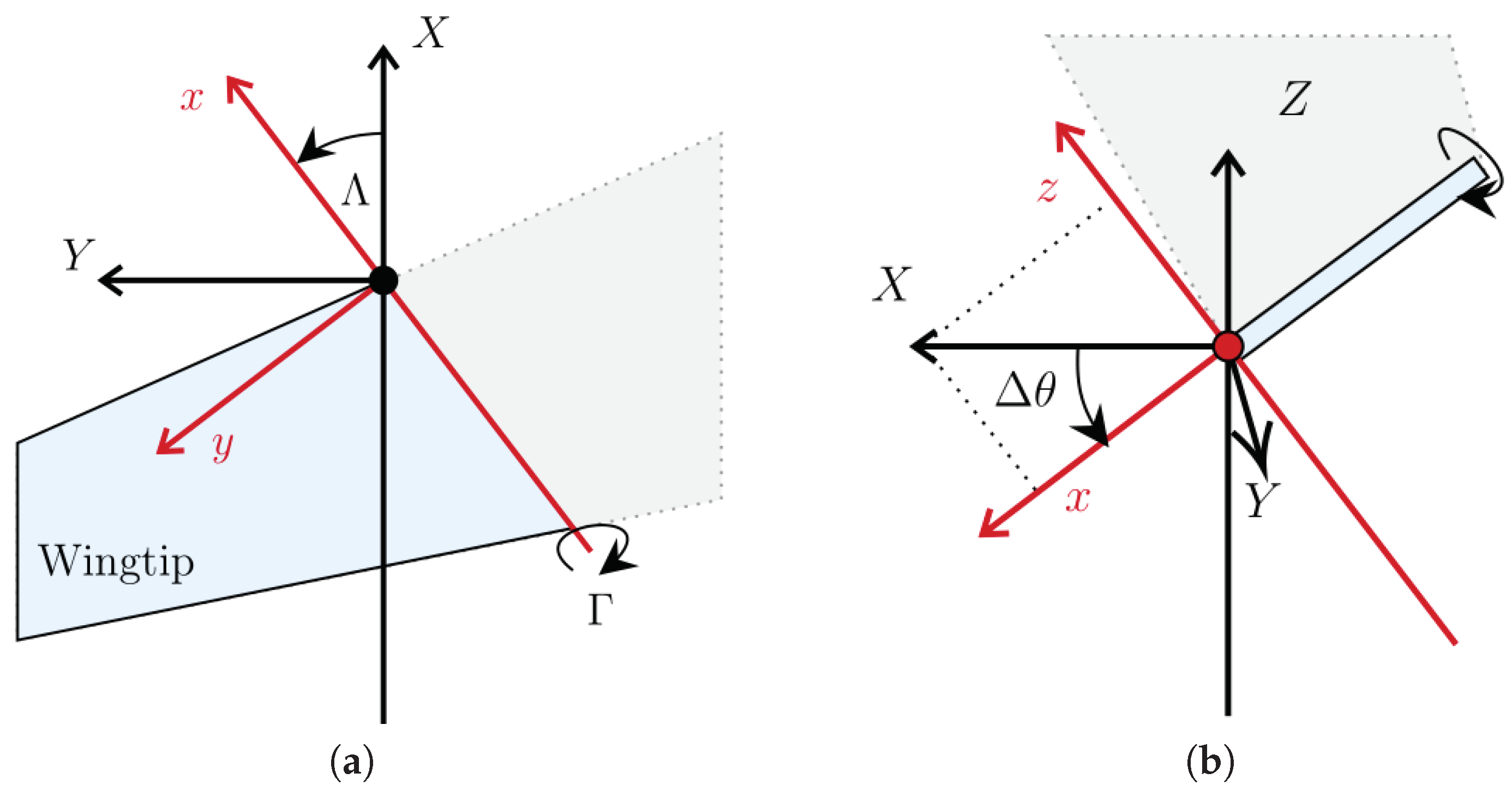
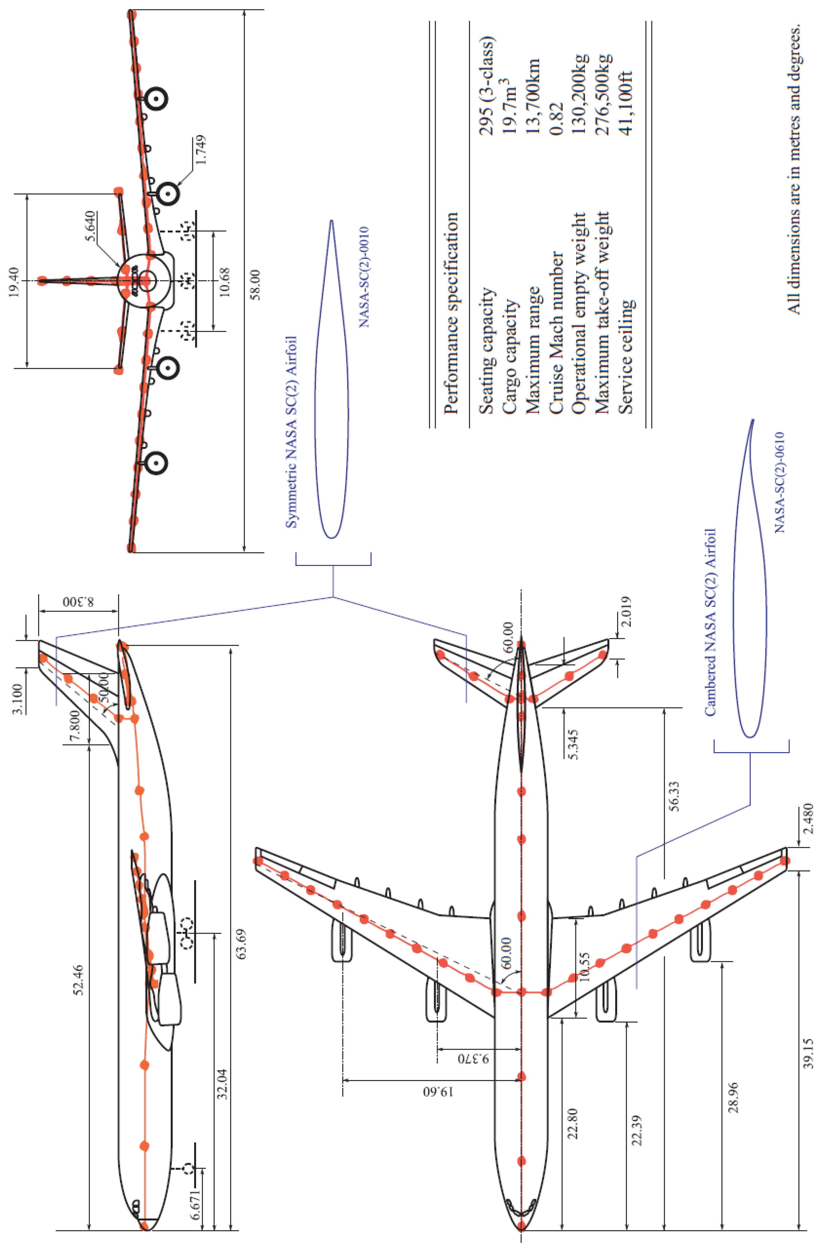
For this case study, a single mass case was considered at approximately 85% of Maximum Take-Off Weight (MTOW) with a Center of Gravity (CoG) at 25% of the mean aerodynamic chord. The wingtip placement corresponded to 10% and 20% of wing semispan from the tip. For the AX-1 aircraft wing span, this corresponds to $2.9$ m and $5.8$ m, respectively. A single hinge flare angle ${\Lambda }_{hinge}={17}^{\circ }$ was used herein. The aircraft was then flown in a finite set of symmetric folding configurations. Values ranging from ${\Gamma }_{wt}=-{20}^{\circ }$ (downward anhedral) to ${\Gamma }_{wt}=+{30}^{\circ }$ (upward dihedral) were used. Note that greater amplitudes would have led to critical local angles of attack beyond realistic stall conditions and limits of the model and were excluded from this investigation. The airframe was also simulated both as a rigid and flexible structure. As the first does not allow for the airframe to change shape under folded or maneuver loads, the comparison highlighted the flexibility effects. A released wingtip configuration was also considered and was limited to flexible structure due to modeling limitations discussed in previous chapters.

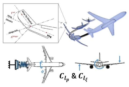
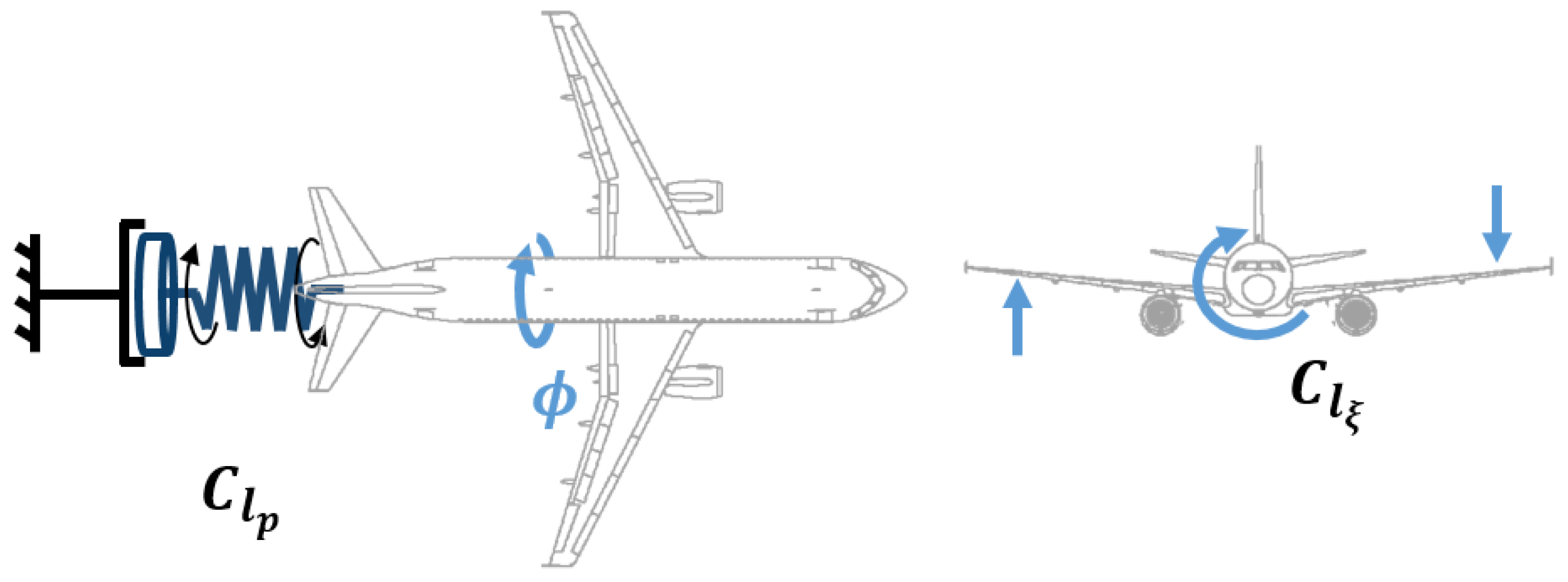
Keeping in mind the mass–spring–damper simplified model, the maneuver can be described as follows [27]. First, as the aileron is deflected asymmetrically, rolling moment is introduced by the overall differential lift from each wing directly highlighting aileron effectiveness $C_{l_{\xi }}$. As the aircraft experiences a controlled rolling moment, additional disturbing moment appears with angular acceleration p. During the roll, the wing undergoes a vertical velocity component (the intensity of which is a function of spanwise coordinate). This in turn, leads to a small increase in local flow incidence on the down-going starboard wing and vice versa on the up going wing. The differential lift gives the restoring rolling moment. The aircraft experiences both the disturbing and restoring rolling moment until a steady roll rate is established. This restoring rolling moment is quantified by the roll damping coefficient, $C_{l_p}$. Lastly, the aircraft roll angle introduces a small but perceivable sideslip angle as the aircraft is not constrained in lateral velocity. This sideslip angle coupled with wing dihedral also leads to differential lift generation, impacting aircraft roll through $C_{l_{\beta }}$.

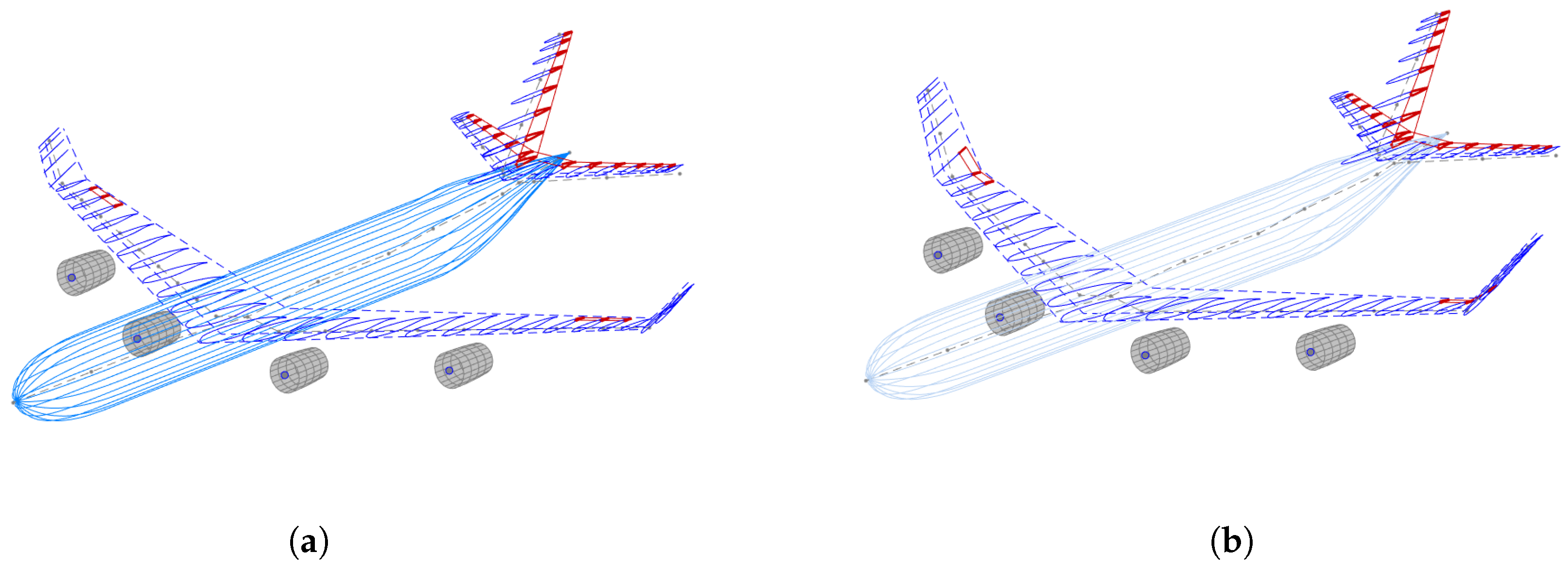
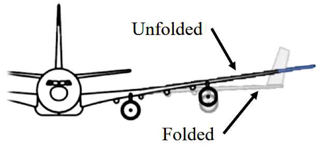
Introducing structural flexibility means that the structure adapts to the external aerodynamic loading and undergoes deformation during perturbation (including aileron input). Different aerodynamic shape therefore lead to changes in differential lift that generates the restoring rolling moment, thus affecting the roll damping $C_{l_p}$ as well as aileron effectiveness $C_{l_{\xi }}$. Figure 6 illustrates, somewhat excessively, the typical shape changes between a folded and baseline wing in a flexible state.

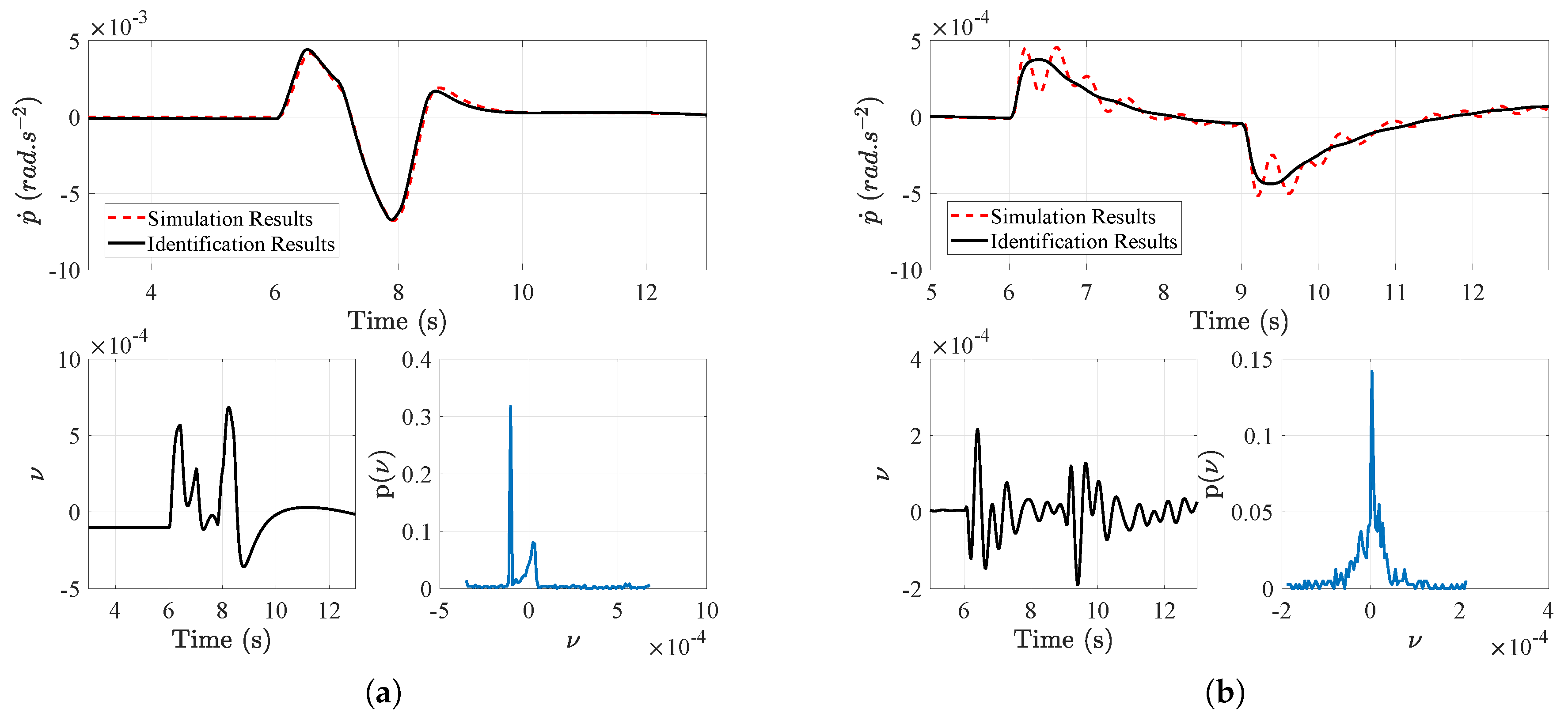
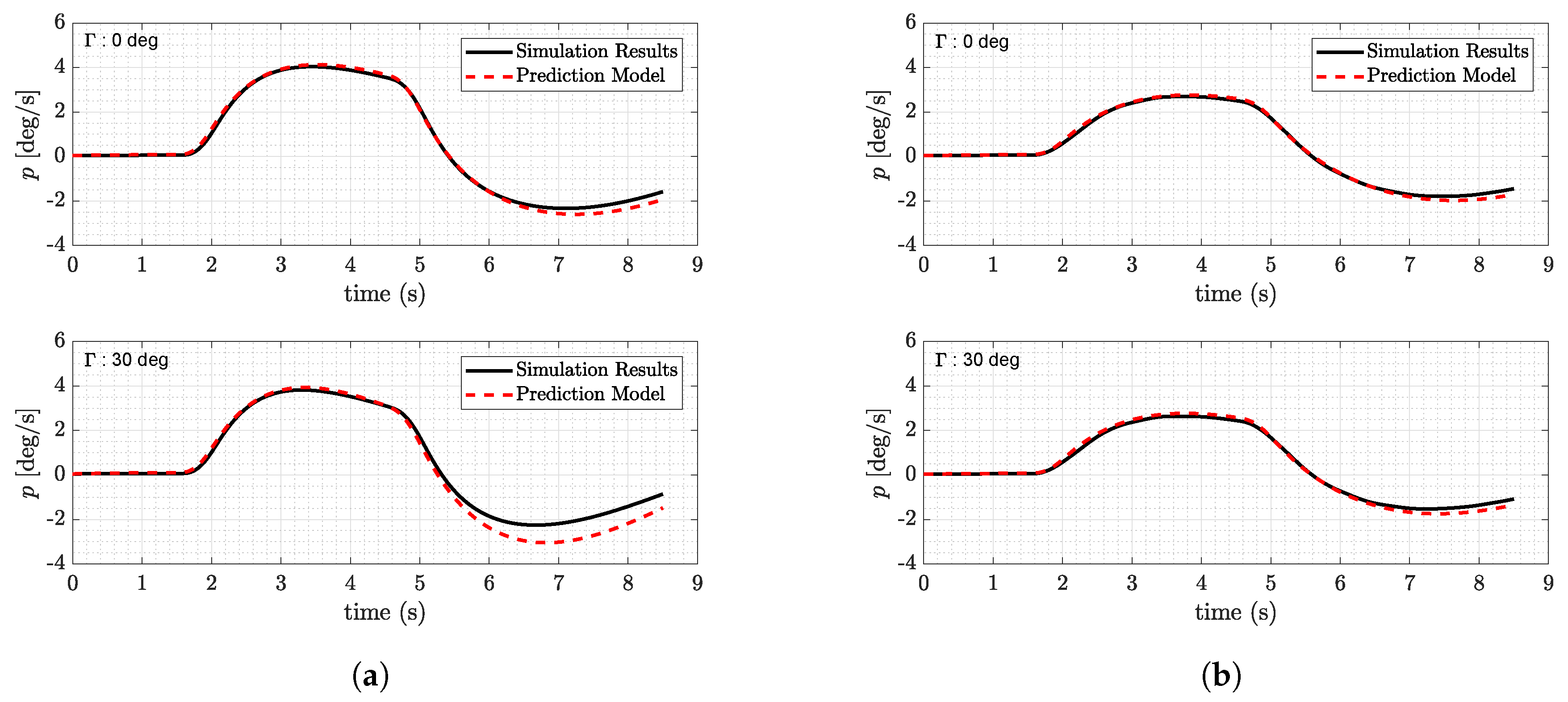
A low amplitude aileron step was used to excite the aircraft roll motion, away from cruise trimmed condition with a non-oscillatory lateral characteristic (additionally, low amplitude aileron doublet and 3-2-1-1 type inputs were used for comparison purposes, although not presented herein). Despite low aileron deflections, steady state roll rate was achieved for the input deflection before large attitude changes were reached. Small perturbations were introduced in the open-loop system, respecting the assumptions required for the systems identification procedure whilst achieving maximum roll rate for a given input which is important for aileron effectiveness identification.

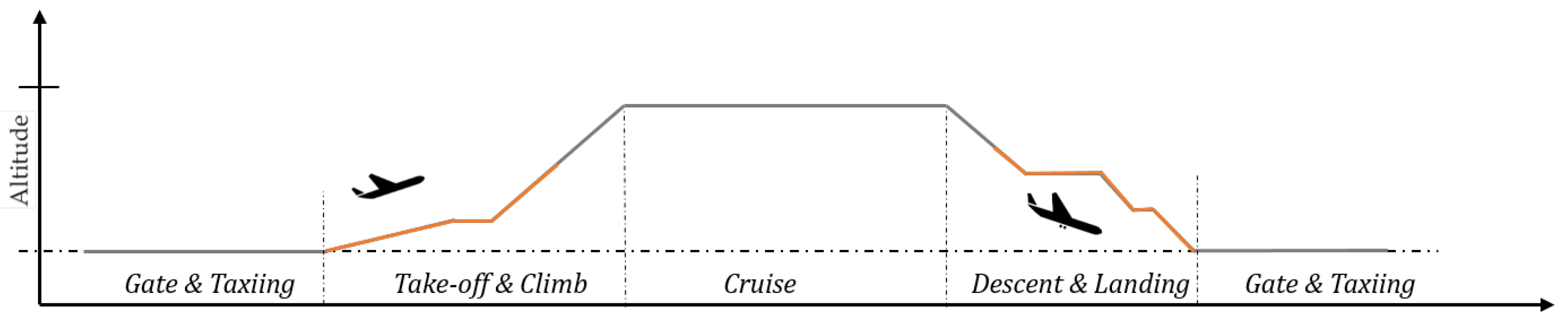
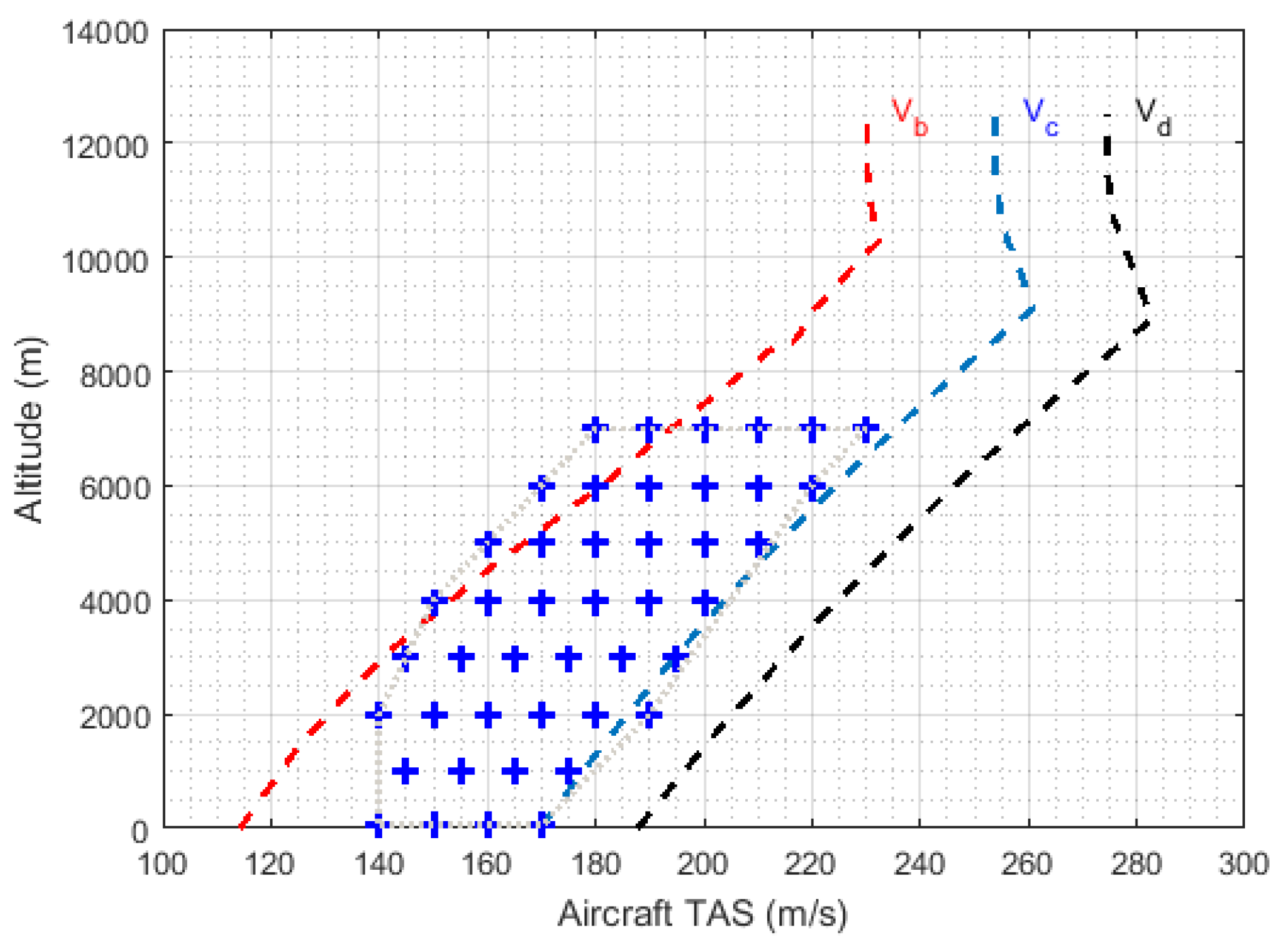
Flight conditions selected for this study correspond to the lower altitude and airspeeds of the AX-1 design envelope so as to match dynamic pressure conditions comparable to “Take-off and Climb”  and “Descent and Landing” conditions, as shown in Figure 7. Figure 8 highlights the 44 flight points selected throughout the flight envelope with ranges of dynamic pressures, altitude and airspeeds experienced at these conditions being given in

Table 1. Range of simulation parameters.

Parameter	Minimum	Maximum
Altitude (m)	50	7000
TAS (m·s ${}^{-1})$	140	230
Mach	$0.41$	$0.74$
$\overline{q}$ (kPa)	$9.2$	$17.2$
${\alpha }_b$ (${}^{\circ }$)	$-0.7$	$2.65$
$R{e}_{root}\times {10}^6$	$6.6$	$11.34$
$R{e}_{hinge}\times {10}^6$	$2.17$	$3.7$

. Additionally, the full set of flight conditions is given in

Table A1. Range of simulation parameters for the entire set of flight conditions considered.

FC	Alt. (m)	$\mathit{\nu }\times {10}^{-5}$ (m${}^2$·s${}^{-1}$)	TAS (m·s${}^{-1}$)	Mach	$\overline{\mathit{q}}$$\left(\mathit{Pa}\right)$	${\mathit{\alpha }}_{\mathit{b}}$${(}^{\circ })$	${\mathit{Re}}_{\mathit{root}}\times {10}^6$	${\mathit{Re}}_{\mathit{hinge}}\times {10}^6$
1	2000	1.715	140	0.42	9863	2.53	7.96	2.6
2	50	1.461	140	0.41	11,947	1.36	9.34	3.05
3	1000	1.581	145	0.43	11,686	1.45	8.94	2.92
4	3000	1.863	145	0.44	9557	2.70	7.59	2.48
5	2000	1.715	150	0.45	11,323	1.60	8.53	2.79
6	4000	2.028	150	0.46	9215	2.91	7.21	2.36
7	50	1.461	150	0.44	13,715	0.85	10.01	3.27
8	1000	1.581	155	0.46	13,354	0.68	9.56	3.12
9	3000	1.863	155	0.47	10,921	1.77	8.11	2.65
10	2000	1.715	160	0.48	12,883	0.82	9.1	2.97
11	4000	2.028	160	0.49	10,485	1.96	7.69	2.51
12	5000	2.211	160	0.5	9422	2.65	7.06	2.3
13	50	1.461	160	0.47	15,605	−0.07	10.68	3.49
14	1000	1.581	165	0.49	15,133	0.03	10.18	3.32
15	3000	1.863	165	0.5	12,375	0.99	8.64	2.82
16	2000	1.715	170	0.51	14,544	0.17	9.66	3.16
17	4000	2.028	170	0.52	11,837	1.17	8.17	2.67
18	5000	2.211	170	0.53	10,637	1.77	7.5	2.45
19	50	1.461	170	0.5	17,616	−0.60	11.34	3.71
20	6000	2.416	170	0.54	9533	2.43	6.86	2.24
21	1000	1.581	175	0.52	17,022	−0.51	10.79	3.52
22	3000	1.863	175	0.53	13,921	0.33	9.16	2.99
23	2000	1.715	180	0.54	16,305	−0.37	10.23	3.34
24	4000	2.028	180	0.55	13,270	0.50	8.65	2.83
25	5000	2.211	180	0.56	11,925	1.03	7.94	2.59
26	6000	2.416	180	0.57	10,687	1.62	7.26	2.37
27	7000	2.646	180	0.58	9550	2.28	6.63	2.17
28	3000	1.863	185	0.56	15,557	−0.23	9.68	3.16
29	2000	1.715	190	0.57	18,167	−0.84	10.8	3.53
30	4000	2.028	190	0.59	14,785	−0.07	9.13	2.98
31	5000	2.211	190	0.59	13,287	0.39	8.38	2.74
32	6000	2.416	190	0.6	11,908	0.91	7.67	2.5
33	7000	2.646	190	0.61	10,640	1.50	7	2.29
34	3000	1.863	195	0.59	17,284	−0.71	10.21	3.33
35	4000	2.028	200	0.62	16,383	−0.55	9.62	3.14
36	5000	2.211	200	0.62	14,722	−0.15	8.82	2.88
37	6000	2.416	200	0.63	13,194	0.31	8.07	2.64
38	7000	2.646	200	0.64	11,790	0.84	7.37	2.41
39	5000	2.211	210	0.66	16,231	−0.60	9.26	3.02
40	6000	2.416	210	0.66	14,546	−0.18	8.47	2.77
41	7000	2.646	210	0.67	12,998	0.29	7.74	2.53
42	6000	2.416	220	0.7	15,965	−0.58	8.88	2.9
43	7000	2.646	220	0.7	14,266	−0.15	8.11	2.65
44	7000	2.646	230	0.74	15,592	−0.50	8.48	2.77

in Appendix C. The aircraft was considered in steady level flight, with a small perturbation introduced to capture lateral dynamics. These conditions can be argued to be similar to loitering motion with large turn radius at constant altitude prior to landing. Climbing and descent flight paths were not considered due to framework trim set-up limitations.

At each of the flight conditions, the aircraft was trimmed in steady level flight in a baseline shape using conventional aircraft controls and no high lift devices (due to current modeling limitations). Trim is achieved after linearization of a reduced-order version of the model (for simplification reasons). An equilibrium (or trim) point was found for each conditions when the steady-state value for each of the state derivatives (with the exception of the aircraft position) was equal to zero (corresponding to steady level flight). When applying symmetric folding input, a correction was applied to the elevator  to balance the pitching moment induced by the deflected wingtips and added to the trimmed elevator deflection.

5.2. Validation of the Identification Process

Figure 9a,b shows a comparison of roll rate acceleration $\dot{p}$ obtained with both the identified state space lateral-directional model and the CA${}^2$LM framework simulation for the rigid and flexible $20\%$ wing semispan wingtip aircraft at ${\Gamma }_{wt}={30}^{\circ }$ deflection. It is clear from these plots that accuracy of the identification is sufficient in the rigid case, throughout the simulation run. On the other hand, structural flexibility leads to oscillations in the CA${}^2$LM results. These oscillations follow a mean trend clearly captured in the identification model. This comes as no surprise as the identification formulation does not capture precisely the wing structural changes of modal shapes $\eta$ and $\dot{\eta }$ and merely compensates in the other terms of the model. Nonetheless, the identified results are satisfactory even in the flexible cases as the general trend is captured with negligible errors $\nu$ and narrow error distributions $p\left(\nu \right)$ (around a null error).

5.3. Aerodynamic Derivative Shift Due to Wingtip Folding

As a result of small perturbation roll maneuver simulations at 44 flight conditions, multiple airframe flexibility and folding angles, an extensive database of $C_{l_p}$ and $C_{l_{\xi }}$ values was generated. This allowed for trends in aerodynamic shifts to be identified. These results were also compared to those of a similar aircraft configuration such as those obtained from flight test campaigns of a Boeing B747 [31] and found to be adequately similar for both $C_{l_p}$ and $C_{l_{\xi }}$. On the other hand, due to the lack of directional coupling and the relatively low sideslip induced during the maneuver, the identification process led to less reliable and higher discrepancy in $C_{l_{\beta }}$ estimates at a number of flight points and overall trends. This effectively led to these results not being included in the following discussion (The authors are investigating alternative inputs and identification method for both $C_{l_{\beta }}$ and $C_{l_r}$ coefficients. Moreover, a coupled lateral-directional mathematical model would be required to adequately capture $C_{l_{\beta }}$, more relevant to coordinated turn (through a combination of rudder and aileron) than roll motion.).

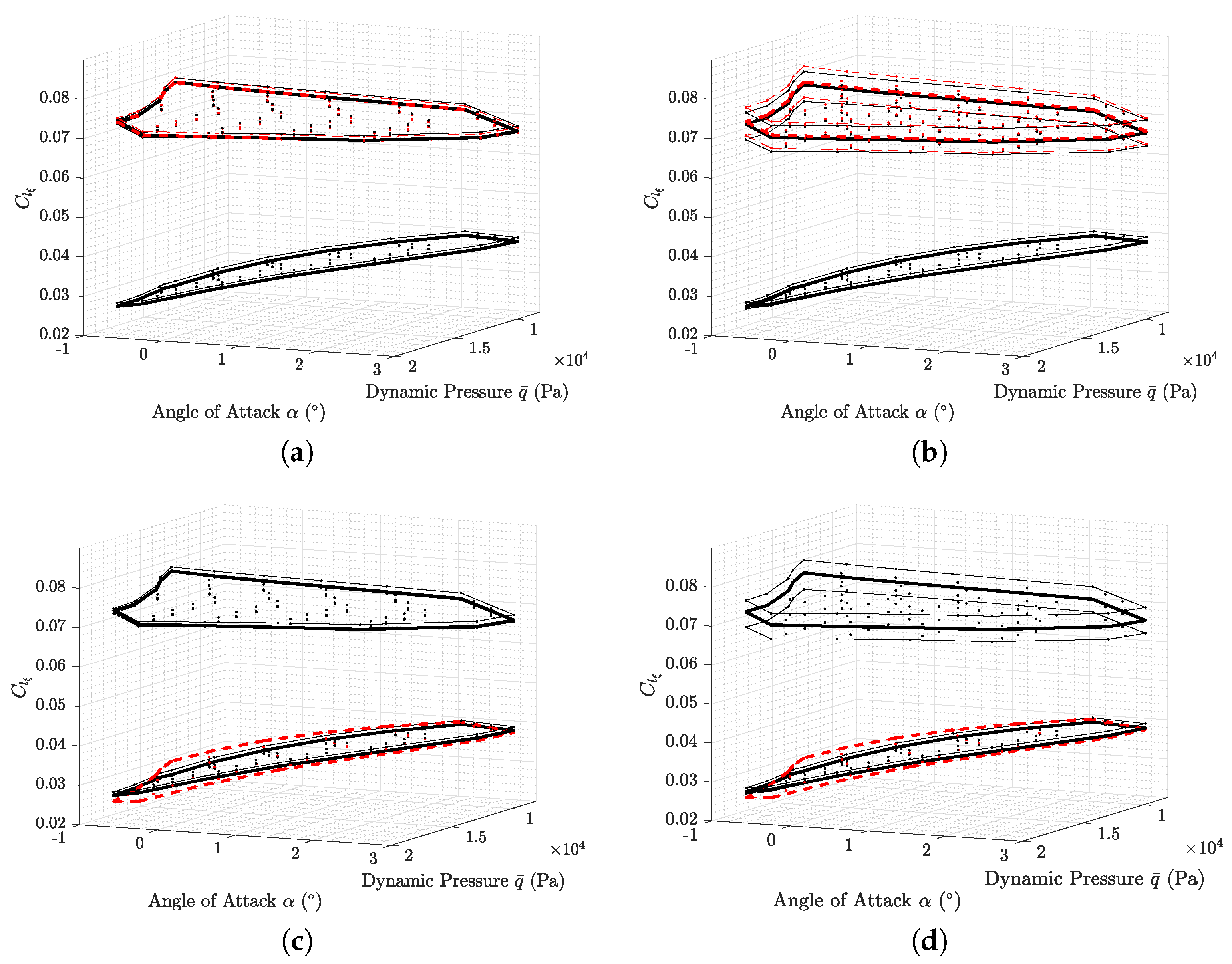
Results presented herein are displayed as a function of both dynamic pressures $\overline{q}$ and angle of attack ${\alpha }_b$, varying over the range of flight conditions. Smooth surface trends are obtained as a function of these two parameters, selected for their relevance to pilots and flight dynamic analysis for further developments. $Re$ could also have been used (replacing $\overline{q}$), although a secondary parameter such as angle of attack would still have been required to better understand the trends captured herein. 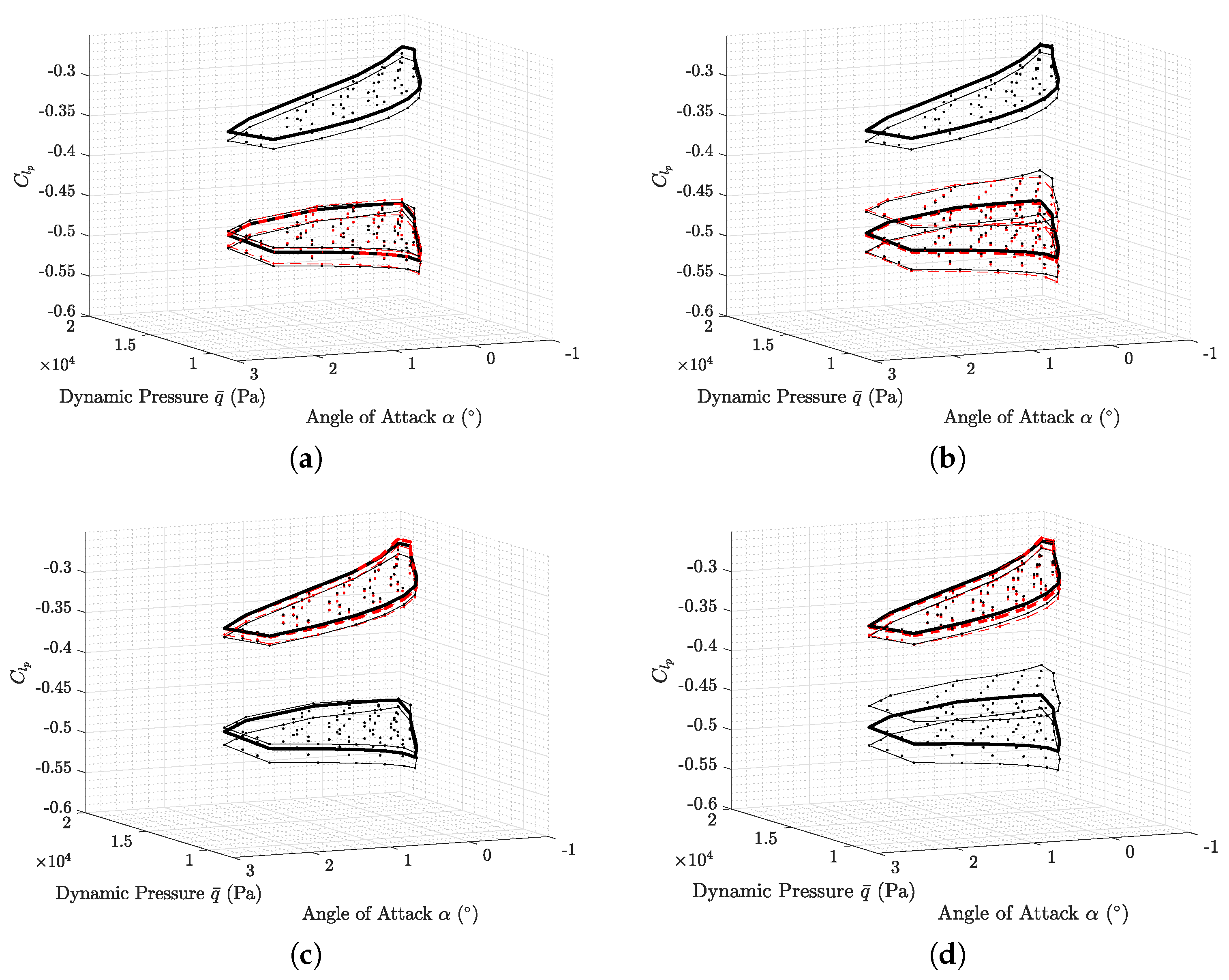Figure 10 and Figure 11 illustrate the trends in aerodynamic derivative changes due to flight conditions. Changes due to wingtip angle effectively lead to a shift of the entire surface as a function of local parameters.

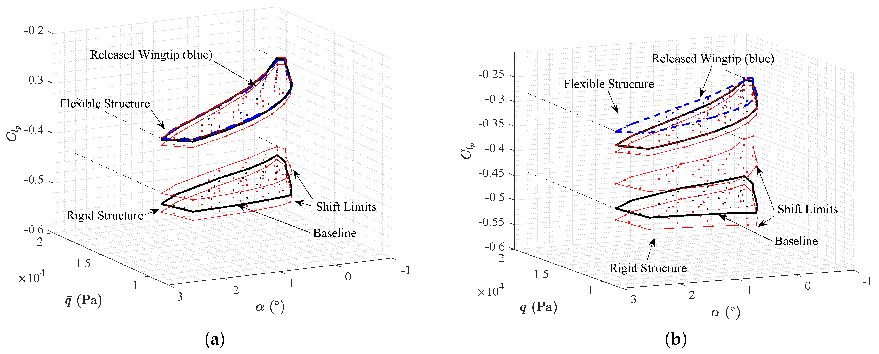
It was found as expected that $C_{l_p}$ values were not only dependent on the aerodynamic shape but also on the flight conditions, as shown in Figure 10b for the larger wingtip variant of the test set-up, where $C_{l_p}$ values for both rigid and flexible airframes in baseline (non folded) and folded configurations are shown. These plots are based on the database generated in the scope of this work, an extract of which is included in Appendix E for the larger wingtip variant. Differences in the baseline $C_{l_p}$ values for both rigid and flexible body structure are obvious and come as a consequence of the change in aerodynamic shape. The latter is changed due to the steady aerodynamic loading as well as the dynamic disturbance (roll rate). Introducing wingtip deflection also changes the aerodynamic loading, particularly tip-loading and overall aerodynamic lift and drag distributions, as shown in Figure 4. On the flexible structure, this forces the structure to adapt and bend, effectively forcing more lift to be generated inboard of the hinge. As a consequence to this phenomenon, relatively small changes are observed on the $C_{l_p}$ value in the flexible case when compared to the rigid structure. In fact, the same can be said for the $C_{l_{\xi }}$ value.

For the rigid aircraft, the $C_{l_p}$ value varies up to 20% relative to the baseline (see Figure 10b or Appendix E) in the worst case for the rigid aircraft. Note that such a change in roll damping is expected to be noticeable by the pilot if it is not corrected through the flight control system, though it should not deteriorate handling qualities to undesirable standard. For the flexible aircraft, a much smaller change of $0.7\%$ is expected at the same flight and folding conditions, with an average of $2\%$ expected in upward folding. Note that the released wingtip cases lead to more noticeable and important $C_{l_p}$ changes of approximately 5–$10\%$.

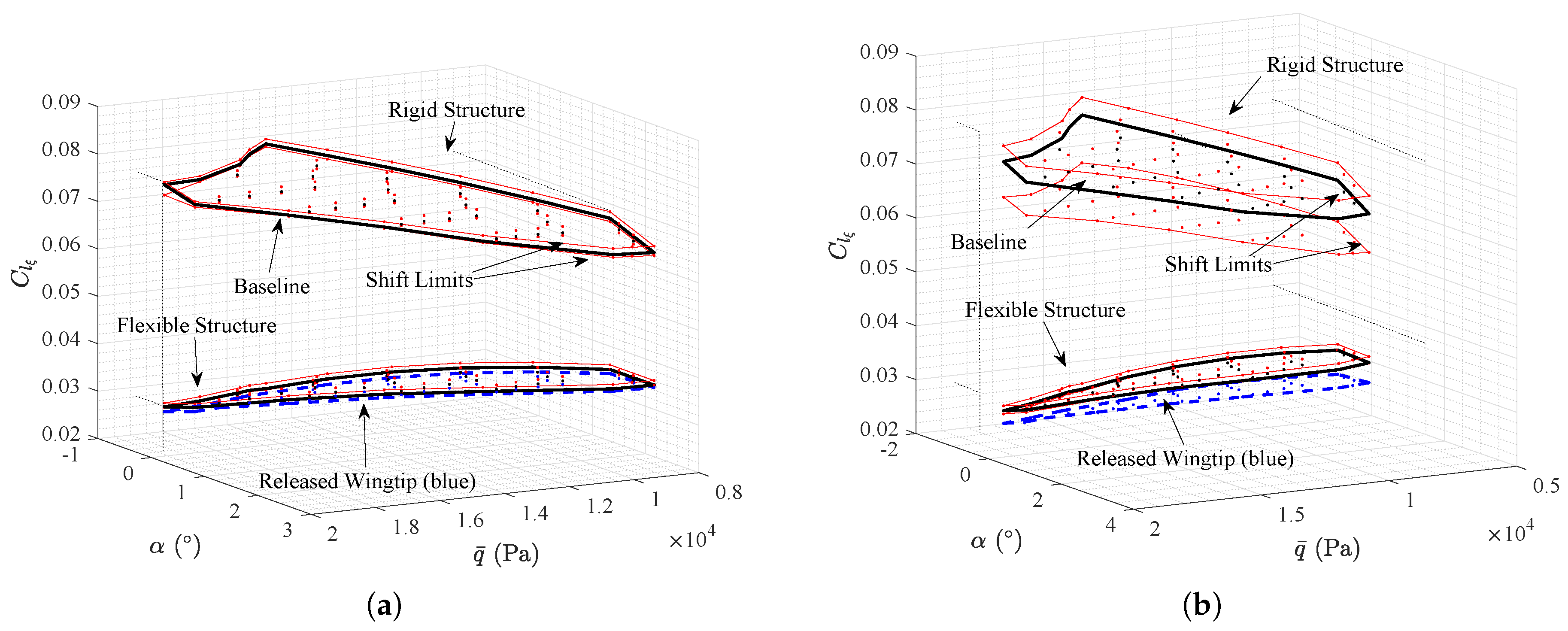
A similar analysis can be made to explain the underlying reasons for the change in $C_{l_{\xi }}$ due to flexibility (and wingtip deflection). Changes in structural flexibility allows the aircraft to adapt to the modified aerodynamic loading and partly counter the effect of the aileron input, thus lowering the $C_{l_{\xi }}$ value compared to that of a rigid aircraft (Figure 11b for the larger wingtips). This phenomenon is not unheard of on very flexible wings where roll control inversion at high dynamic pressures have already been discussed. Similarly, small changes to aileron effectiveness are introduced with wingtip deflections. On the other hand, for the rigid body simulation set, the location of aileron and wingtip hinge line significantly impact the resulting $C_{l_{\xi }}$ value. In the $10\%$ wing semispan wingtip, the outboard limit to the aileron is far enough from the hinge line ($2.9$ m) so that the wingtip deflection does not significantly impact the flow around the aileron. Aileron aerodynamics are not affected significantly. On the other hand, the $20\%$ wing semispan wingtip size case introduces a hinge nearly overlapping with the aileron outboard limit. Nonetheless, changes to aileron effectiveness remain relatively low with fold angle, with shifts ranging between $4\%$ and $-2\%$ in both upward and downward deflections. On the other hand, the change in aerodynamic loading on the aileron during wingtip release leads to a significant change in $C_{l_{\xi }}$ value, with a maximum decrease of $12\%$ relative to the baseline (Figure 11b) in aileron authority, linked by the authors to flapping wingtip effects. For the rigid case, a change between $+5\%$ and $-8\%$ is introduced.

A quick look at the results presented in Figure 10 and Figure 11 can lead to the following statement: a greater change in roll dynamics is introduced when shifting from rigid to flexible airframe, than when flying the aircraft with different fold angles throughout the flight envelope. Thus, it can be stated that switching from a rigid to a flexible aircraft would prove by far more challenging to a pilot than the folding of the wingtips themselves.Additionally, it also shows that the wing flexibility greatly dampens or reduces the wingtip folding effects. In the case of a very rigid wing, the controlled folding of the wingtips would have a greater impact on the aircraft response, as shown by the rigid simulations given herein. These are very promising results for further development of the design as a lower impact of wingtip folding on the handling qualities of a flexible aircraft might lead to positive pilot perception of the system and relatively minor flight control law changes (at least for lateral control) can be expected.

Additionally, the authors believe that it is relevant to state that the released or loose wingtip state appears in this study as most suitable for roll performances: with a decreased roll damping and only slight reduction in aileron authority, the authors believe that loose wingtips could be efficiently used during maneuvers to restore some roll performances lost by increasing the aircraft span in the case of a HARW concept. Note that, with lower roll damping, the upward fold of the wingtip for a rigid aircraft gives a more suitable shape for roll maneuvers. With increasing wing flexibility, this effect can dissipate, as seen herein. Note that aircraft range or climb performance are not considered and should also be taken into account when considering suitable wingtip or winglet designs.

6. Prediction Model Derivation

The results from the identification process could be implemented directly in a flight simulator model or database to capture the impact of wingtip folding on the aircraft flight dynamics. However, this requires significant effort in terms of data transfer and implementation, for each aircraft and/or wingtip device. An alternative identified by the authors would be to implement a correction or prediction model to account for the effect of folding wingtips on the aerodynamic derivatives as a function of simulation conditions. From previous results, it was found that the difference or shift between baseline and folded configurations can be parametrized as a function of flight condition, wingtip size, and folding angle. Hence, such a prediction model could be built around the baseline rigid body configuration for example and apply corrections to key aerodynamic derivatives as a function of flight conditions and wingtip parameters. The appropriate shift or $\Delta C_l$ could therefore be predicted without the needs for complex physics based models (as used in CA${}^2$LM) or extensive databases in the aerodynamic derivative based simulators.

From findings presented in Section 5, such prediction models were hypothesized by the authors with the following formulation:

$$\begin{array}{cc}\hfill C_{l_p}^{\Gamma }& ={C_{l_p}^{\Gamma =0}}_{\mathrm{rigid}}\left(1+\Delta C_{l_p}(\Gamma ,\varsigma ,\overline{q})\right)\hfill \end{array}$$

(9)

$$\begin{array}{cc}\hfill C_{l_{\xi }}^{\Gamma }& ={C_{l_{\xi }}^{\Gamma =0}}_{\mathrm{rigid}}\left(1+\Delta C_{l_{\xi }}(\Gamma ,\varsigma ,\overline{q})\right)\hfill \end{array}$$

(10)

As such, simple polynomial formulations are used to compute the output variables ($C_{l_p}$ and $C_{l_{\eta }}$) based on the following independent variables: $\Gamma$, the wingtip deflection in radians; $\varsigma$, the position of the hinge line from wingtip as a fraction of the wingspan (0.1 for 10% hinge line and 0.2 for 20% hinge line); and $\overline{q}$, aircraft dynamic pressure in kg·m${}^{-1}$·s${}^{-2}$. The reader should note that a common problem encountered when deriving such polynomial models relates to the selection of the terms which should be included in the model for a given set of data, also known as model structure determination.

In this particular study, the prediction model was obtained using a non-linear multivariate orthogonal identification approach, which was used through the mof function [28]. The process generates non-linear orthogonal modeling functions from the independent variables data and uses the functions to build an adequate model based on the predicted mean square error metric. The identified orthogonal function model can then be converted to a multivariate ordinary polynomial expansion. This model is not only concise but also gives physical insight into the identified functional dependencies. Once the polynomial function is fixed, the parameters are identified based on least-squares estimation. Details of the algorithm can be found in Morelli et al. [28,29] and other use cases [32].

Utilising the mof function, polynomial dependencies to the independent variables was limited to terms of order 3 or less, with only $\Gamma$ raised to the ${\Gamma }^3$ dependency. Based on this assumption, the global equation for the model structure is defined in Equations (11) and (12), while the coefficients identified are presented in

Table 2. Prediction model derivation.

		${\mathit{a}}_1$	${\mathit{a}}_2$	${\mathit{a}}_3$	${\mathit{a}}_4$	${\mathit{a}}_5$	${\mathit{a}}_6$	${\mathit{a}}_7$
$C_{l_p}$	rigid	-	-	−1.137	−1.677	0.079	0.250	−0.184
	flexible	−0.134	$-1.65\times {10}^{-5}$	−0.174	-	-	0.095	-
		${\mathit{b}}_{\mathbf{1}}$	${\mathit{b}}_{\mathbf{2}}$	${\mathit{b}}_{\mathbf{3}}$	${\mathit{b}}_{\mathbf{4}}$	${\mathit{b}}_{\mathbf{5}}$	${\mathit{b}}_{\mathbf{6}}$	${\mathit{b}}_{\mathbf{7}}$
$C_{l_{\xi }}$	rigid	-	-	−1.133	0.296	0.087	0.065	-
	flexible	−0.179	$-2.67\times {10}^{-5}$	-	-	-	-	-

.

$$\begin{array}{cc}\hfill \Delta C_{l_p}(\Gamma ,\varsigma ,\overline{q})& =a_1+a_{2}q+\left(a_3\Gamma +a_4{\Gamma }^2\right)\varsigma +a_5\Gamma +a_6{\Gamma }^2+a_7{\Gamma }^3\hfill \end{array}$$

(11)

$$\begin{array}{cc}\hfill \Delta C_{l_{\xi }}(\Gamma ,\varsigma ,\overline{q})& =b_1+b_{2}q+\left(b_3\Gamma +b_4{\Gamma }^2\right)\varsigma +b_5\Gamma +b_6{\Gamma }^2+b_7{\Gamma }^3\hfill \end{array}$$

(12)

The coefficient presented in Table 2 show that the prediction model used to introduce flexible structure based on the rigid body aerodynamic derivatives is mainly a function of dynamic pressure $\overline{q}$. The results also suggest that, in the case of a flexible structure, the wingtip did not lead to changes in the $C_{l_{\xi }}$ value. On the other hand, the $C_{l_p}$ values for a flexible aircraft change with respect to wingtip size $\varsigma$ and wingtip deflection $\Gamma$. In fact, a second-order term and therefore non-linear dependency to the wingtip deflection is highlighted. For the rigid structure configuration, the roll damping $C_{l_p}$ and aileron effectiveness $C_{l_{\xi }}$ are highly dependent on both wingtip size and deflection. The $C_{l_p}$ shows a cubic dependency with the wingtip deflection, while the $C_{l_{\xi }}$ only has a quadratic relation with the wingtip deflection. Once again, cubic relations were chosen as the maximum order to consider non-linearity without leading to an over parameterized model. A comparison between the updated aerodynamic derivatives using the prediction model and the identification results obtained from CA${}^2$LM  simulations is made in Figure 12 and Figure 13. The black lines show the identified variables from parameter identification, while the red lines highlight the prediction model results. Overall, the prediction model captures the variation in $C_{l_p}$ and $C_{l_{\xi }}$ very well with respect to wingtip deflections ($\Gamma$) and flexibility effect (although only quasi-steady effects are effectively captured).

To validate the prediction model further, a state space model based on Equation (7) and $C_{l_p}$ and $C_{l_{\xi }}$ values from the prediction model and compared against CA${}^2$LM results. $C_{l_r}$ is ignored, while $\beta$ and $\xi$ are treated as inputs. Figure 14 shows a comparison between the state space model (prediction) and the CA${}^2$LM  framework for a flight at 180 m·s${}^{-1}$, h = 10,000 ft, with $\xi =5^{\circ }$ aileron input held for 5 s. It should be noted that this flight condition is not part of the set used to develop the prediction model but lies well within the envelope for interpolation. The match between the resulting time histories from both CA${}^2$LM  and the prediction models was found to be satisfactory for the aircraft response to such an aileron deflection. Results for the rigid structure show a slight deviation in response during recovery of the turn (after the initial input). A reason for this is the difference in degrees of freedom between the two simulations: CA${}^2$LM  results are based on 6 DoF equations of motion while the prediction model is only 1 DoF in rolling, which neglects the lateral-directional coupling. The difference comes from the sideslip angle, which in this case is treated as an input for both models, and plays a significant role in the rigid body case.

Overall, these results highlight that changing the aircraft roll dynamic response through aerodynamic derivatives using a polynomial correction model from baseline to morphed configurations leads to very similar results to the original 6 DoF non-linear flexible airframe simulations. The advantage of the first over the latter is clear, as the polynomial formulation is much more easily implemented in a flight simulator environment for pilot-in-the-loop simulations without requiring physics based model, as implemented in the more complex CA${}^2$LM framework. Hence, the authors  believe that the use of such an approach could be beneficial if appropriately implemented.

7. Conclusions and Further Work

A folding mechanism was initially introduced within the CA${}^2$LM aeroservoelastic simulation framework to investigate the impact of folding wingtips on the roll dynamics of a large generic flexible aircraft. The aircraft roll response was therefore investigated for a range of flight conditions within the nominal flight envelope of the civil aircraft aircraft selected for this analysis. A couple of different wingtip parameters were compared based on ground folding size requirements. For comparative purposes, the airframe was simulated as either rigid or flexible in different simulation sets.

A parameter identification method was applied to extract the aircraft roll dynamics as a function of wingtip angle and flight conditions, with aircraft roll damping $C_{l_p}$ and aileron effectiveness $C_{l_{\xi }}$ aerodynamic derivatives presented herein. Results for the baseline configuration (no wingtip deflection) were found to be similar to that of a comparable sized aircraft (the Boeing B747 [31] was used as a reference). The change in roll dynamics due to wingtip folding were less important when the airframe was given realistic flexibility, as the wing shape adapted to changes in aerodynamic loading. For the larger wingtip variant, both downward and upward deflections led to increases in $C_{l_p}$ amplitude of $4\%$ and $2\%$, respectively, whilst a released wingtip led to a decrease in amplitude ranging between $5\%$ and $10\%$ when compared to the baseline at similar flight conditions. For $C_{l_{\xi }}$, an average increase of $3\%$ and $1.5\%$ for downward and upward deflections, respectively, was introduced, whilst an average decrease of $10\%$ emerged when releasing the wingtips. For the rigid structure, trends were found to be different due to the lack of wing deflection changes and lift distribution differences induced by wingtip folding, with $C_{l_p}$ modifications ranging from $-5\%$ (downward) to $+12\%$ (upward) and $+5\%$ and $-7\%$ for $C_{l_{\xi }}$. Accurate numbers for these comparisons can be found in Appendix E, which includes an extract of the database generated in the scope of this work. The reader should note that, in fact, the average difference between rigid and flexible aircraft derivatives at similar flight and wingtip conditions (approximately at $50\%$ difference for $C_{l_p}$ and $100\%$ for $C_{l_{\xi }}$ scaled against flexible data) were found to be greater throughout the range of tested positions and flight conditions than the shifts experienced throughout the test conditions. This result is not unexpected for large tubular body with swept wing configurations, and points to less drastic consequences of in-flight folding wingtips on flight dynamics when flexibility is considered for swept wing aircraft. Thus, it can be stated that switching from a rigid to a flexible aircraft would prove by far more challenging to a pilot than the folding of the wingtips themselves.

Overall, an aerodynamic derivative database was generated in order to be implemented to an engineering flight simulator, an extract of which is included in Appendix E. However, to avoid a long and tedious manual implementation process (valid only for a given aircraft and wingtip system), a set of lateral aeroderivatives prediction models were developed instead. By taking into account flexibility, wingtip deflection, wingtip size and flight conditions as input parameters, these models help predict the dynamic response of an aircraft with in-flight wingtip folding by using a correction or $\Delta C_l$ formulation to a conventional aeroderivative based flight dynamics model. As a result, two prediction models were developed for flexible and rigid configurations, applicable over a wide range of flight conditions and folding angles. Adequate correlation between the physics based folding model in CA${}^2$LM and the corrective prediction model applied to a linear state space formulation were found. These prediction models will then be implemented in a Cranfield Engineering Flight Simulator for pilot-in-the-loop investigations aimed at assessing the impact of wingtip folding on the aircraft handling qualities.

As this paper focuses only on the roll dynamics of the aircraft, an extensive list of further work should be considered. Firstly, a single mass case, center of gravity position and flare angle were used herein. This must be extended further to validate the predictive model approach and allow for more reliable pilot-in-the-loop simulations for correct handling qualities investigations. Moreover, the quantification of the wingtip roll, yaw or pitch control derivative (similar to the aileron, rudder and elevator) could also be of interest. Additionally, the authors noted that directional and longitudinal motion of the aircraft are also greatly influenced by wingtip folding and therefore require further investigations. The coupling of these dynamics in the system identification process applied to CA${}^2$LM is therefore a logical next step to capture the resulting coupled motion of the aircraft, making the identification of important additional lateral derivatives such as $C_{l_{\beta }}$ and $C_{l_r}$ more accurate and reliable. Finally, the identification of the aircraft aerodynamic derivatives in conditions different to steady level flight (investigated herein) such as steady climb, descent or a banking turn (to mimic loiter, for instance) would also be interesting to capture the shifts in derivatives of interest, if significant, due to other flight phase conditions.

References

1. Dussart, G.; Yusuf, S.; Lone, M. Effect of wingtip morphing on the roll mode of a flexible aircraft. In Proceedins of the AIAA/ASCE/AHS/ASC Structures, Structural Dynamics, and Materials Conference, Kissimmee, FL, USA, 8–12 January 2018; American Institute of Aeronautics and Astronautics: Reston, VA, USA, 2018. [Google Scholar] [CrossRef]
2. Castrichini, A.; Siddaramaiah, V.H.; Calderon, D.E.; Cooper, J.E.; Wilson, T.; Lemmens, Y. Nonlinear folding fing tips for gust loads alleviation. J. Aircr. 2016, 53, 1391–1399. [Google Scholar] [CrossRef]
3. Castrichini, A.; Siddaramaiah, V.H.; Calderon, D.E.; Cooper, J.E.; Wilson, T.; Lemmens, Y. Preliminary Investigation of Use of Flexible Folding Wing-Tips for Static and Dynamic Loads Alleviation. Aeronaut. J. 2017, 121, 73–94. [Google Scholar] [CrossRef]
4. Dussart, G.; Yusuf, S.; Portapas, V.; Lopez, G.; Lone, M. Method to assess lateral handling qualities of aircraft with wingtip morphing. In Proceedings of the AIAA Aeroelasticity and Flight Dynamics Conference, AIAA SciTech Forum, Kissimmee, FL, USA, 8–12 January 2018. [Google Scholar] [CrossRef]
5. Allerton, D. Principles of Flight Simulation; John Wiley & Sons: Chichester, West Sussex, UK, 2009; p. 471. ISBN 0470682191. [Google Scholar]
6. Lockheed Martin Official Website. 2014. Available online: https://www.lockheedmartin.com/us/news/features/2014/5-unique-f35c-carrier-variant-features.html (accessed on 1 December 2017).
7. Bradley, M.K.; Droney, C.K. Subsonic Ultra Green Aircraft Research: Phase II: N + 4 Advanced Concept Development; Technical Report NASA/CR-2012-217556; NASA: Hanover, MD, USA, 2012.
8. Hayes, D.; Lone, M.; Whidborne, J.; Coetzee, E. Evaluating the rationale for folding wing tips comparing the exergy and Breguet approaches. In Proceedings of the 55th AIAA Aerospace Sciences Meeting, Grapevine, TX, USA, 9–13 January 2017. [Google Scholar] [CrossRef]
9. Kamlet, M.; Gibbs, Y. NASA Tests New Alloy to Fold Wings in Flight; NASA: Edwards, CA, USA, 2018.
10. Pace, S. North American XB-70 Valkyrie; Aero Series #30; Aero Publishers: New York, NY, USA, 1990; p. 98. ISBN 0830686207. [Google Scholar]
11. Jenkins, D.R.; Landis, T. North American XB-70A Valkyrie; Specialty Press: Thurgoona, Australia, 2002; p. 104. ISBN 1580070566. [Google Scholar]
12. Dussart, G.; Lone, M.; O’Rourke, C.; Wilson, T. In-flight folding wingtip system: Inspiration from the XB-70 Valkyrie. Morphing Wings II. In Proceedings of the AIAA SciTech Forum, San Diego, CA, USA, 7–11 January 2019. [Google Scholar] [CrossRef]
13. Bourdin, P.; Gatto, A.; Friswell, M.I. Aircraft control via variable cant-angle winglets. J. Aircr. 2008, 45, 414–423. [Google Scholar] [CrossRef]
14. Mills, J.; Ajaj, R. Flight dynamics and control using folding wingtips: An experimental study. Aerospace 2017, 4, 19. [Google Scholar] [CrossRef]
15. Kandath, H.; Pushpangathan, J.; Bera, T.; Dhall, S.; Bhat, M.S. Modeling and closed loop flight testing of a fixed wing micro air vehicle. Micromachines 2018, 9, 111. [Google Scholar] [CrossRef] [PubMed]
16. Andrews, S.P. Modelling and Simulation of Flexible Aircraft: Handling Qualities with Active Load Control. Ph.D. Thesis, Cranfield University, School of Engineering, Bedford, UK, 2011. [Google Scholar]
17. Dussart, G.; Portapas, V.; Pontillo, A.; Lone, M. Flight dynamic modelling and simulation of large flexible aircraft. In Flight Physics—Models, Techniques and Technologies; InTech: London, UK, 2018. [Google Scholar] [CrossRef]
18. Leishman, J.G.; Nguyen, K.Q. State-space representation of unsteady airfoil behaviour. AIAA J. 1990, 28, 836–844. [Google Scholar] [CrossRef]
19. Leishman, J.G.; Beddoes, T.S. A generalised model for airfoil unsteady aerodynamic behaviour and dynamic stall using the indicial method. In Proceedings of the 42nd Annual forum, Washington, DC, USA, 2–4 June 1986. [Google Scholar]
20. Lone, M. Pilot Modelling for Airframe Loads Analysis. Ph.D. Thesis, Cranfield University, School of Aerospace, Transport and Manufacturing, Bedford, UK, 2013. [Google Scholar]
21. Lone, M.; Dussart, G. Impact of spanwise non-uniform discrete gusts on civil aircraft loads. Aeronaut. J. 2019, 123, 93–120. [Google Scholar] [CrossRef]
22. Portapas, V.; Cooke, A.K.; Lone, M. Modelling framework for flight dynamics of flexible aircraft. Aviation 2016, 20, 173–182. [Google Scholar] [CrossRef]
23. Carrizales, M.; Dussart, G.; Portapas, V.; Pontillo, A.; Lone, M. Comparison of reduced order aerodynamic models and RANS simulations for whole aircraft aerodynamics. In Proceedings of the AIAA Atmospheric Flight Mechanics Conference, Kissimmee, FL, USA, 8–12 January 2018. [Google Scholar] [CrossRef]
24. Lone, M.; Cooke, A. Pilot-model-in-the-loop simulation environment to study large aircraft dynamics. J. Aerosp. Eng. 2012, 227, 555–568. [Google Scholar] [CrossRef]
25. Lone, M.; Lai, C.K.; Cooke, A.; Whidborne, J. Framework for flight loads analysis of trajectory-based manoeuvres with pilot models. J. Aircr. 2014, 51, 637–650. [Google Scholar] [CrossRef]
26. Waszak, M.R.; Buttril, C.S.; Schmidt, D.K. Modeling and Model Simplification of Aeroelastic Vehicles: An Overview; Technical Report; National Aeronautics and Space Administration: Hampton, VA, USA, 1992. [Google Scholar]
27. Cook, M.V. Flight Dynamics Principles: A Linear Systems Approach to Aircraft Stability and Control, 3rd ed.; Elsevier Aerospace Engineering Series; Butterworth-Heinemann: Oxford, UK, 2013; ISBN 978-0-08-098242-7. [Google Scholar]
28. Klein, V.F.; Morelli, E.A. Aircraft System Identification. Theory and Practice; AIAA Education Series; AIAA: Reston, VA, USA, 2006; ISBN 9781563478321. [Google Scholar]
29. Morelli, E.A.; DeLoach, R. Wind tunnel database development using modern experiment design and multivariate orthogonal functions. In Proceedings of the 41st Aerospace Sciences Meeting and Exhibit, Reno, NV, USA, 6–9 January 2003. [Google Scholar] [CrossRef]
30. Jategaonkar, R.V. Flight Vehicle System Identification: A Time Domain Methodology; AIAA: Reston, VA, USA, 2006; p. 534. [Google Scholar] [CrossRef]
31. Heffley, R.K.; Jewell, W.F. Aircraft Handling Qualities Data; Technical Report; NASA: Washington, DC, USA, 1972.
32. Yusuf, S.; Chavez, O.; Lone, M. Application of multivariate orthogonal functions to identify aircraft flutter modes. In Proceedings of the AIAA Atmospheric Flight Mechanics Conference, AIAA SciTech Forum, Grapevine, TX, USA, 9–13 January 2017. [Google Scholar] [CrossRef]
Figure 1. Scope of the aerodynamic derivative coefficient identification.
Aerospace 06 00063 g001
Figure 2. Flared dihedral folding wingtip mechanism: (a) sketch of the morphing wingtip geometry; and (b) local twist modification Δ θ w t with Γ w t and Λ h i n g e .
Aerospace 06 00063 g002
Figure 3. Discretized reduced order model representations of the AX-1 aircraft: (a) 2.9 m wingtip (10% semispan), 1 beam–5 aerodynamic stations wingtip; and (b) 5.8 m wingtip (20% semispan), 2 beam–8 aerodynamic stations wingtip.
Aerospace 06 00063 g003
Figure 4. Wingtip folding angle Γ w t effect on AX-1 vertical force coefficient with a flared hinge: (a) 20% wing semispan wingtip—rigid; and (b) 20% wing semispan wingtip—flexible.
Aerospace 06 00063 g004
Figure 5. Illustrations of equivalent mass–spring–damper roll model.
Aerospace 06 00063 g005
Figure 6. Wing shape adaptation due to flexibility and wingtip folding.
Aerospace 06 00063 g006
Figure 7. Full mission profile with critical test cases (orange) during “Take-off and Climb” and “Descent and Landing”.
Aerospace 06 00063 g007
Figure 8. Selected flight conditions.
Aerospace 06 00063 g008
Figure 9. SID match for p ˙ of the AX-1 with 20 % wingtip (aileron step input, T A S = 200 m·s 1 and h = 4575 m): (a) Γ w t = 30 rigid; and (b) Γ w t = 30 flexible.
Aerospace 06 00063 g009
Figure 10. C l p variations against q ¯ and α b : (a) 2.9 m (10% wing semispan) wingtip device; and (b) 5.8 m (20% wing semispan) wingtip device.
Aerospace 06 00063 g010
Figure 11. C l ξ variations against q ¯ and α b : (a) 2.9 m (10% wing semispan) wingtip device; and (b) 5.8 m (20% wing semispan) wingtip device.
Aerospace 06 00063 g011
Figure 12. Roll damping model (black: identified model, red: prediction model): (a) rigid model 10% wingtip; (b) rigid model 20% wingtip; (c) flexible model 10% wingtip; and (d) flexible model 20% wingtip.
Aerospace 06 00063 g012
Figure 13. Aileron effectiveness model (black: identified model, red: prediction model): (a) rigid model 10% wingtip; (b) rigid model 20% wingtip; (c) flexible model 10% wingtip; and (d) flexible model 20% wingtip.
Aerospace 06 00063 g013
Figure 14. Prediction model and CA 2 LM simulation comparison for a validation of the 20% semispan wingtip device results: (a) rgid model 20% wingtip; and (b) flexible model 20% wingtip.
Aerospace 06 00063 g014