1. Introduction
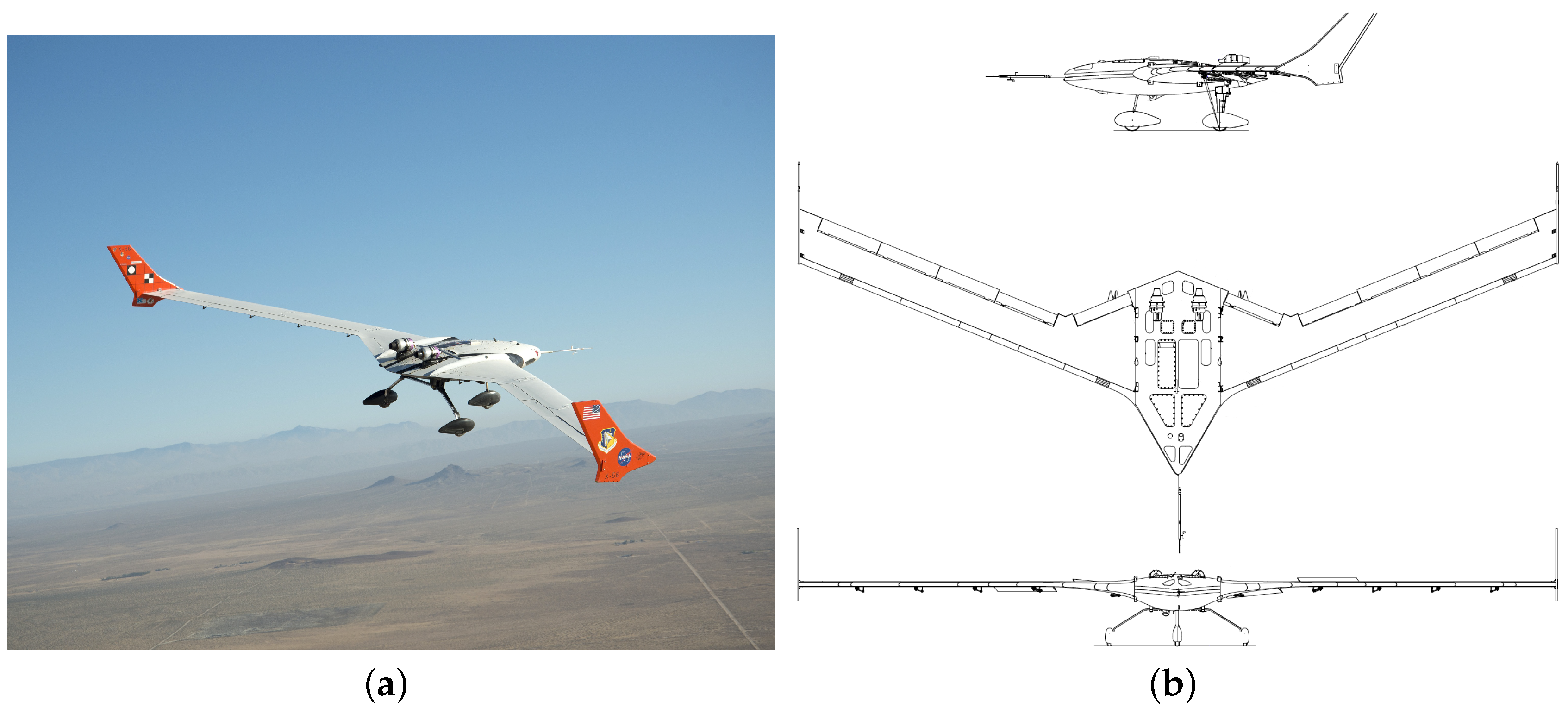
Efforts to reduce fuel consumption and increase aerodynamic efficiency of aircraft can lead to vehicle designs having long and slender wings. Such airplanes may experience aeroelastic effects in flight, potentially resulting in performance degradation, structural fatigue, or catastrophic loss of aircraft. To mature modeling and control technologies for flexible aircraft and mitigate these effects, the NASA Advanced Air Transport Technology (AATT) Project has been conducting flight research with the X-56A Multi-Utility Technology Testbed (MUTT) aircraft [
1], which was purposefully designed to encounter aeroelastic instabilities within its normal flight envelope [
2].
For flight dynamics analysis, a useful model for predicting and understanding the behavior of flexible aircraft is the work of Waszak and Schmidt, which was first presented in Reference [
3] and elaborated upon in References [
4,
5,
6,
7]. Their work extended traditional rigid-body flight dynamics models based on quasi-steady stability and control derivatives (for example, Reference [
8]) to include a mean-axis reference frame with generalized modal vibration states and aeroelastic derivatives that couple the aerodynamics and the structural deformation. The Waszak–Schmidt model is applicable for small, linear flight variable perturbations and elastic deformations. Similar to standard flight-dynamics models, it assumes quasi-steady aerodynamics; any unsteady effects are lumped into the aeroelastic stability derivatives. It also assumes that the structural deformation of the aircraft can be decomposed into a superposition of orthogonal vibration modes. Despite these limitations, the Waszak–Schmidt model is applicable in a large number of cases, particularly the aeroelastic analysis of the X-56A flight test data. Furthermore, the Waszak–Schmidt model is representative of the observed flight motions, including near flutter, and is of relatively low order, making it useful for flight dynamics analyses and feedback control design.
The Waszak–Schmidt model or similar models have been used in system identification analyses to estimate aeroelastic stability and control derivatives from flight test data. In Reference [
9], low-order transfer functions are fit to frequency responses computed from flight test data of the XV-15 tiltrotor VTOL aircraft. In References [
10,
11,
12], state-space models are fit to computed frequency responses for a large transport aircraft, a YAV-8B Harrier, and a mid-sized business jet. In each of these works, it is argued that, because the lowest vibration mode is at least five times the highest rigid-body mode of interest, the stability and control derivatives that couple the elastic motion of the aircraft to the rigid-body equations of motion can be neglected. This is a simplification of the Waszak–Schmidt model, called the hybrid-flexible model, wherein the structural deformations of the aircraft are registered in the sensor measurements but otherwise do not impact the gross motion of the vehicle. This simplified model is also used in Reference [
13], where the filter-error approach is used to identify models for the SR-71 aircraft from measured time histories. In Reference [
14], the full Waszak–Schmidt model is used to identify a model of a high-performance glider using an output-error analysis in the time domain. In References [
15,
16], flight data from frequency sweeps and multisine inputs are used with output-only modal identification and frequency response estimation to identify aeroelastic models of a small, unmanned aircraft. Grauer and Boucher [
17] proposed a real-time method based on state reconstruction and the equation-error approach in the frequency domain, and demonstrated the method using X-56A flight test data. In Reference [
18], a state-space implementation of the Waszak–Schmidt model is used to fit computed frequency response data of the X-56A operating under closed-loop control with input mixing. Additional case studies in the literature, including less recent works, are summarized in Reference [
19].
The aforementioned examples of system identification using aeroelastic flight dynamics models are relatively few compared to the existing literature for rigid-body flight dynamics models. One reason for this disparity is the difficulty in accurately identifying aeroelastic models. In particular, the model size can become very large and incorporate many inputs, outputs, states, and unknown model parameters. Because vibration modes of the aircraft structure can occur at relatively high frequencies, faster sampling rates and higher-quality hardware are needed to obtain adequate modeling data. The necessity to excite a broad range of frequencies, to identify responses from many control effectors, and to estimate a large number of model parameters can result in long data records to achieve the requisite level of data information. All these factors result in computationally intensive system identification analyses. Furthermore, the modal states of the aircraft structure are not directly observable but indirectly affect many of the output response measurements. In addition to the mass and inertia properties needed to identify rigid-body models, structural properties such as modal frequencies and modes shapes must be measured, modeled, or estimated from the data. Lastly, many estimation methods are nonlinear and require iteration from good starting values. Although there is a large body of knowledge for stability and control derivatives of conventional aircraft and rigid-body models, the aeroelastic derivatives are less familiar and can require a separate analysis to obtain appropriate values. Each of these characteristics makes the system identification problem more difficult for flexible aircraft models than for rigid-body models.
In this paper, a different approach for testing flexible aircraft and identifying model parameters is discussed. Orthogonal phase-optimized multisine inputs were used to simultaneously excite multiple control effectors on the X-56A over specified bandwidths and with prescribed power spectra. This step led to an efficient flight test maneuver with good data for linear modeling. Using the Waszak–Schmidt model structure, the output-error approach for parameter estimation was applied to fit Fourier transforms of measured output responses. This approach avoided the need for direct state measurements, incorporated data from numerous inputs and outputs over frequency ranges of interest, provided physical insights from the frequency-domain perspective, and reduced the size of the optimization problem needed to estimate stability and control derivatives. The method is restricted to linear models describing small perturbations and deformations about a reference flight condition, such as those typically used in a flutter analysis, and needs good starting values for the model parameters, which were provided by a numerical panel code.
This paper is organized as follows. In
Section 2, the X-56A aircraft, flight-test instrumentation, and structural characteristics are discussed.
Section 3 details the experiment design, including the orthogonal phase-optimized multisine inputs used to excite the aircraft. The Waszak–Schmidt aeroelastic flight dynamics model used for identification is summarized in
Section 4, and the output-error approach using frequency-domain data is discussed in
Section 5. Then,
Section 6 presents the identification results and characteristics of the identified model. Conclusions are drawn in
Section 7.
Due to ITAR restrictions associated with the X-56A airplane, numerical values are not given in this paper. However, the approach is general and not specific to this aircraft or configuration. Routines for the experiment design, data analysis, and system identification are from the MATLAB
®-based software package called System IDentification Programs for AirCraft (SIDPAC) [
20].
3. Experiment Design
The system identification maneuvers consisted of trimming the aircraft in straight and level flight and then applying excitations on the control surfaces. Because there are many control surfaces, a large frequency bandwidth of interest, many test points, and a relatively fast rate of fuel consumption affecting the mass and aeroelastic properties properties of the aircraft, testing using conventional inputs on sequential control surfaces would have been prohibitive. Instead, orthogonal phase-optimized multisine inputs were used to move all the control surfaces at the same time, but in different ways, over a specified frequency band and with prescribed power spectra. The orthogonal phase-optimized multisine inputs (hereafter referred to as multisines) summarized in this section were first presented in References [
24,
25] and were elaborated upon in Reference [
22] and the references therein.
Multisine input design begins with choosing the time duration
T, which defines the fundamental frequency
. Harmonic frequencies
for integer values of
are then selected to span the bandwidth of interest. For
different inputs to be excited at the same time, the harmonics in
K are divided among the subsets
,
, …,
. The multisines for each input are then assembled as
which are summations of harmonic sinusoids. The power spectra
can take a uniform distribution to excite all the harmonic frequencies equally, which is the usual case, or can be designed to emphasize or avoid different modal responses. The
values for each input are also jointly scaled to achieve responses with good signal-to-noise ratios. The phase spectra
for each input are optimized using a simplex method for the minimum relative peak factor (RPF)
resulting in inputs that generate small perturbation responses about the flight condition, appropriate for linear modeling. Because the sinusoids used in Equation (
1) are harmonic multiples, they are mutually orthogonal; therefore, the multisines can be used on multiple control surfaces at the same time without correlating the input data. This property allows flight test time to be considerably reduced by exciting multiple control effectors at the same time instead of in sequence. The multisines are added to other inputs from the pilot and control system just before the actuators. A feedback control law will raise the level of correlation between the inputs, but when configured in this manner, input pairwise correlations remain well below the 0.9 guideline suggested in Reference [
22] and facilitate accurate estimation of the bare-airframe dynamics using the output-error approach. The actual model structure to be identified is not important at this point (beyond that the relevant dynamics are well excited); rather, it is only important that the inputs are sufficiently different so that the responses resulting from each input can be distinguished.
For the X-56A Phase 1 flight tests, 72 different multisine inputs were designed for identification of the bare-airframe dynamics using different combinations of control surfaces and engine throttles for various amplitudes and frequency ranges. For the excitation discussed in this paper (flight test aid (FTA) 506), the control surfaces on the left and right wings were moved symmetrically. For example, the symmetric body flap deflections were defined as
where the “
s” subscript stands for symmetric. This setup resulted in five multisines for the symmetric control surface pairs. The time duration
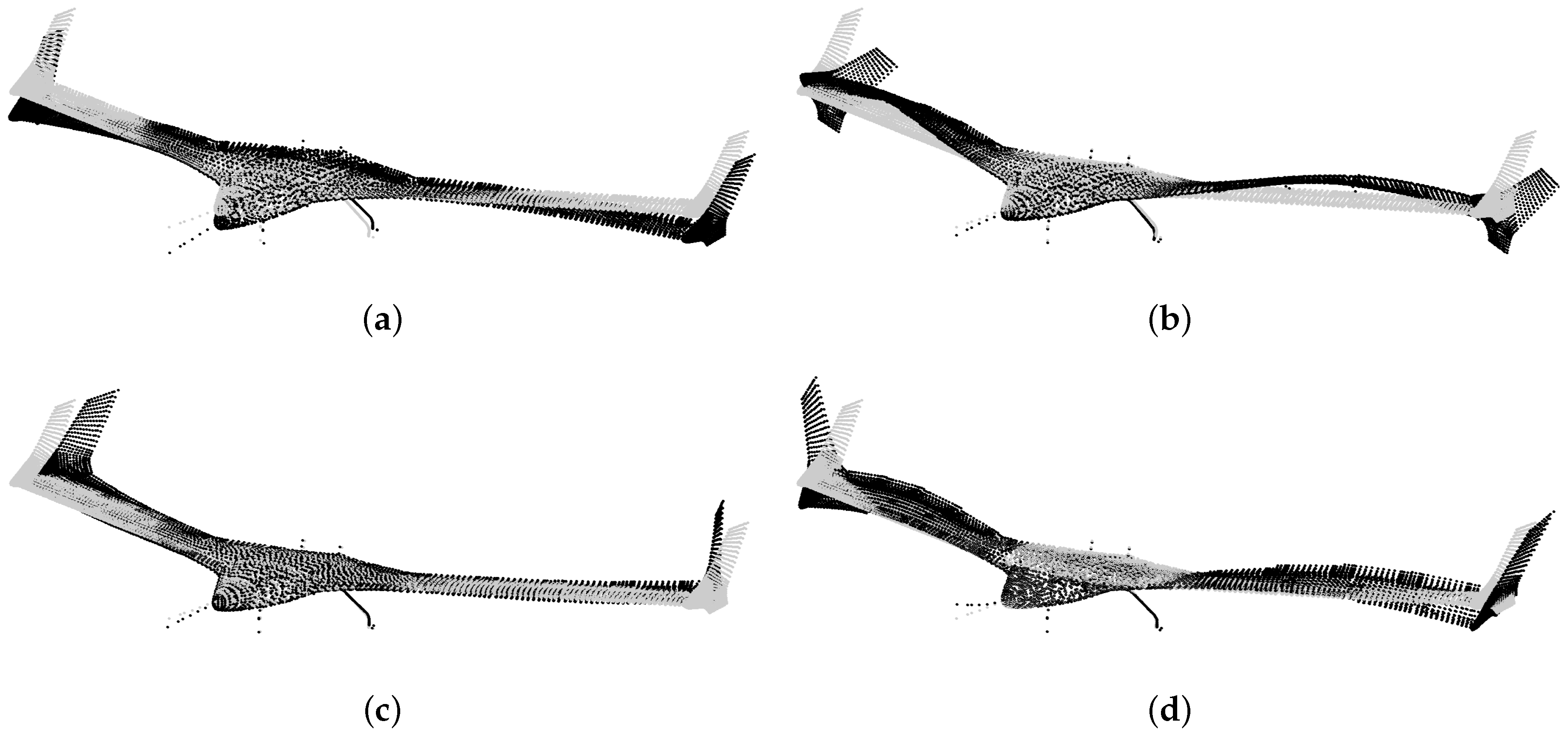
T was chosen to produce a short maneuver with adequate frequency resolution over the modal responses of interest for five inputs. The adequacy of the frequency resolution was confirmed prior to flight testing using the nonlinear simulation, and the estimated changes in mass properties were judged to be sufficiently small for linear modeling. The bandwidth of the included harmonic frequencies spanned short period (SP) mode and the four vibration modes shown in
Figure 2. In total, 325 harmonic frequencies were used, with 65 frequencies on each input. The ordering of the frequencies among the five inputs was:
,
,
,
, and
, which ensured that sequential frequencies were distributed over the wing and not excited on neighboring control surfaces. The power spectra for these multisines were uniform in frequency, and the amplitudes were adjusted using a nonlinear simulation of the aircraft to attain good expected signal-to-noise ratios under a variety of conditions.
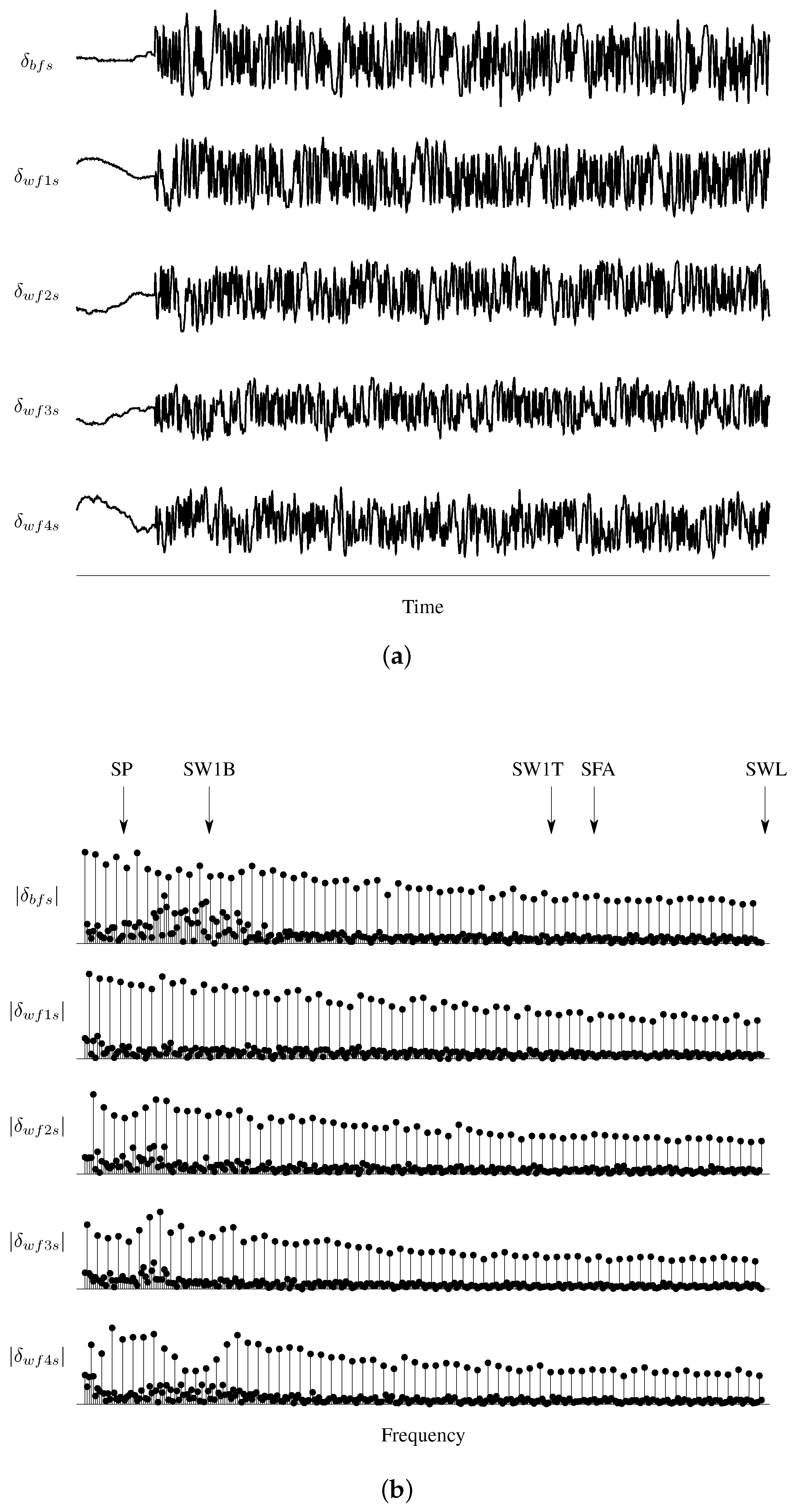
Measurements of control surfaces deflections are shown in
Figure 4a. The maneuver contained approximately 2.5 cycles of the input, but only one cycle is shown for clarity. The y-axes have the same sizes but different mean values for each input. These measurements include not only the multisine perturbation inputs, but also contributions from the pilot and control system. In the first part of the maneuver before the excitation onset, the aircraft is essentially trimmed and the relatively low-frequency movement of the control surfaces is from the control system. The multisines were designed to be orthogonal but the control mixing and feedback raised the maximum control surface correlation to
. This correlation was well below the 0.9 guideline and was not an issue during the identification analysis.
Fourier transforms of the measured control surface data (computed using the method discussed later in
Section 5) are shown as amplitude spectra in
Figure 4b. The transforms were only evaluated at the harmonic frequencies used in the multisine inputs. This choice restricted the number of frequency-domain data points to those having the input power, thereby reducing the computational complexity of the analysis without reducing the amount of information in the modeling data. Modeling results did not significantly improve with more frequency points. The ranges for the axes in each plot again have the same scale. Resonant frequencies for the short period and in-vacuo structural modes are annotated in
Figure 4b. The actuator bandwidth created some amplitude attenuation with increasing frequency. Although the inputs were designed to have unique frequencies for each control surface, control mixing and feedback control changed the frequency content near the short period and SW1B modes for
,
,
, and
.
5. Output-Error Parameter Estimation in the Frequency Domain
The output-error approach for parameter estimation is the maximum likelihood estimator for dynamic systems where process noise (for example, turbulence) is neglected. A set of unknown model parameters are determined that best match the model outputs to measured output data. For this analysis, the outputs were Fourier transforms of the aircraft responses and the model parameters were non-dimensional stability and control derivatives in the Waszak–Schmidt model. A brief summary of the output-error approach using frequency-domain data, based on References [
22,
27], is presented in this section.
To perform the estimation in the frequency domain, the finite Fourier transform
is used to convert detrended time-domain data into frequency-domain data, where
T is the time duration of the data record of
and where
is the radian frequency. Fast Fourier transforms (FFTs) could be used to implement the Fourier transform, but these have relatively coarse frequency resolution for aircraft flight dynamics applications. Rather, Equation (
21) can be computed to arbitrary resolution and a high degree of accuracy using the chirp z-transform and cubic interpolation of the time series data [
22,
28]. Because the Fourier transform is a linear operator, dynamic models used in frequency-domain output error are restricted to linear systems. However, this is a mild restriction in this case because the flight test data involved small-perturbations about a reference flight condition and were represented well using linearized models.
Applying the Fourier transform to the state-space model assembled from Equations (
8) and (
16) yielded the input-output relation
in the frequency domain assuming zero initial conditions. The measured output was modeled as
where the additive measurement noise
had
where
is the spectral density of
and where
N is the number of frequencies analyzed.
The maximum likelihood cost function to be minimized for the unknown model parameters in the output-error approach with frequency-domain data is
where
is the vector of unknown model parameters and the residuals are
In the past, attempts to minimize the cost function in Equation (
25) for both
and
at the same time have led to convergence problems. To overcome this, a relaxation technique is typically employed to alternate solving between one of these two unknowns while holding the other constant. This technique has been shown to work well in practice.
For a given
, minimizing the cost function for the residual spectral density matrix leads to
While holding this matrix constant, Equation (
25) can then be minimized for the model parameters as
Optimization of Equation (
28) can be done iteratively from starting values for the model parameters using the Gauss–Newton method. This technique is similar to the Newton–Raphson method but does not require the Hessian matrix to be computed. The iteration update for the model parameters is
The matrix
is the Fisher information matrix, where
is the output sensitivity matrix, which can be computed analytically by taking derivatives of Equation (
22) as
or numerically using finite differences. If the sensitivities are computed using the analytical derivatives, the state solution used in Equation (
32) is
similar to Equation (
22). The optimization runs faster using analytical derivatives rather than numerical derivatives because obtaining finite differences requires perturbing each of the many unknown model parameters and computing the outputs. In Equation (
29), the matrix
is the cost function gradient. The uncertainty in the estimated parameters is given by the Cramér–Rao bounds
where the square root of the diagonal elements are the standard errors.
Of the many techniques for parameter estimation, output error has many benefits. First, it has a strong theoretical underpinning based in maximum likelihood, and has been used extensively for decades. The assumptions used in output error are physically relevant and reflect flight testing in calm weather. The analysis can incorporate many sensors and can be used with states that are not directly observable, such as the modal displacements and rates. Drawbacks of using output error include that starting values are needed for the unknown model parameters, iterations are required for the nonlinear optimization, and additional effort is needed to change the structure of the model.
Performing the modeling using frequency-domain data also has many benefits. First, viewing the data in the frequency domain provides insight into the modal resonances of the system, such as the structural modes. Second, the computational analysis runs faster in the frequency domain than the time domain, especially when analytically-derived sensitivity equations are used. One reason for this is that the equations of motion are solved in the frequency domain using addition and multiplication, per Equation (
22), rather than in the time domain using convolution. Another reason is that there are typically fewer data points to process in the frequency domain than in the time domain. A third reason is that because bias and trend information is removed from the data before applying Fourier transforms, biases in the state and output equations are not estimated. These factors reduce the total number of parameters to be estimated and lessens the computation time required for each optimization iteration. Lastly, analysis with output error in the frequency domain does not require any corrections to the estimated uncertainty levels, which is usually done with time-domain data to correct for colored residuals not assumed by the theory. The frequency-domain output-error analysis is restricted to linear systems, but this was not a drawback for the results presented in this paper because the maneuvers involved small perturbations about a reference condition.
6. Results
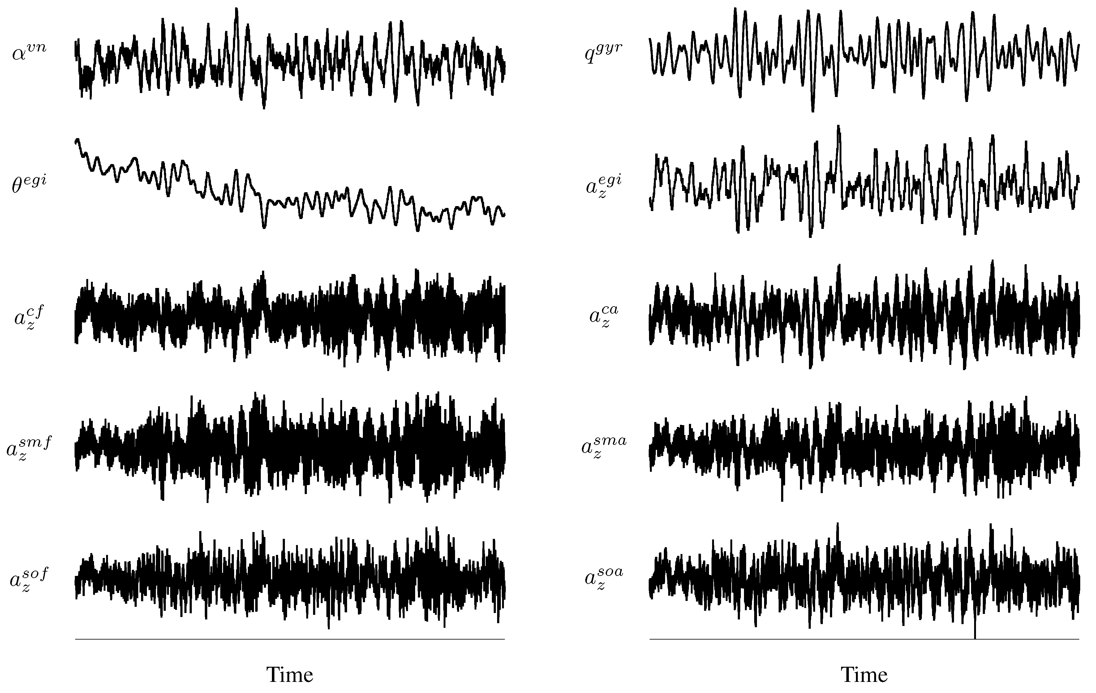
Measured outputs for the identification maneuver are shown in
Figure 5. The inputs for this maneuver are shown in
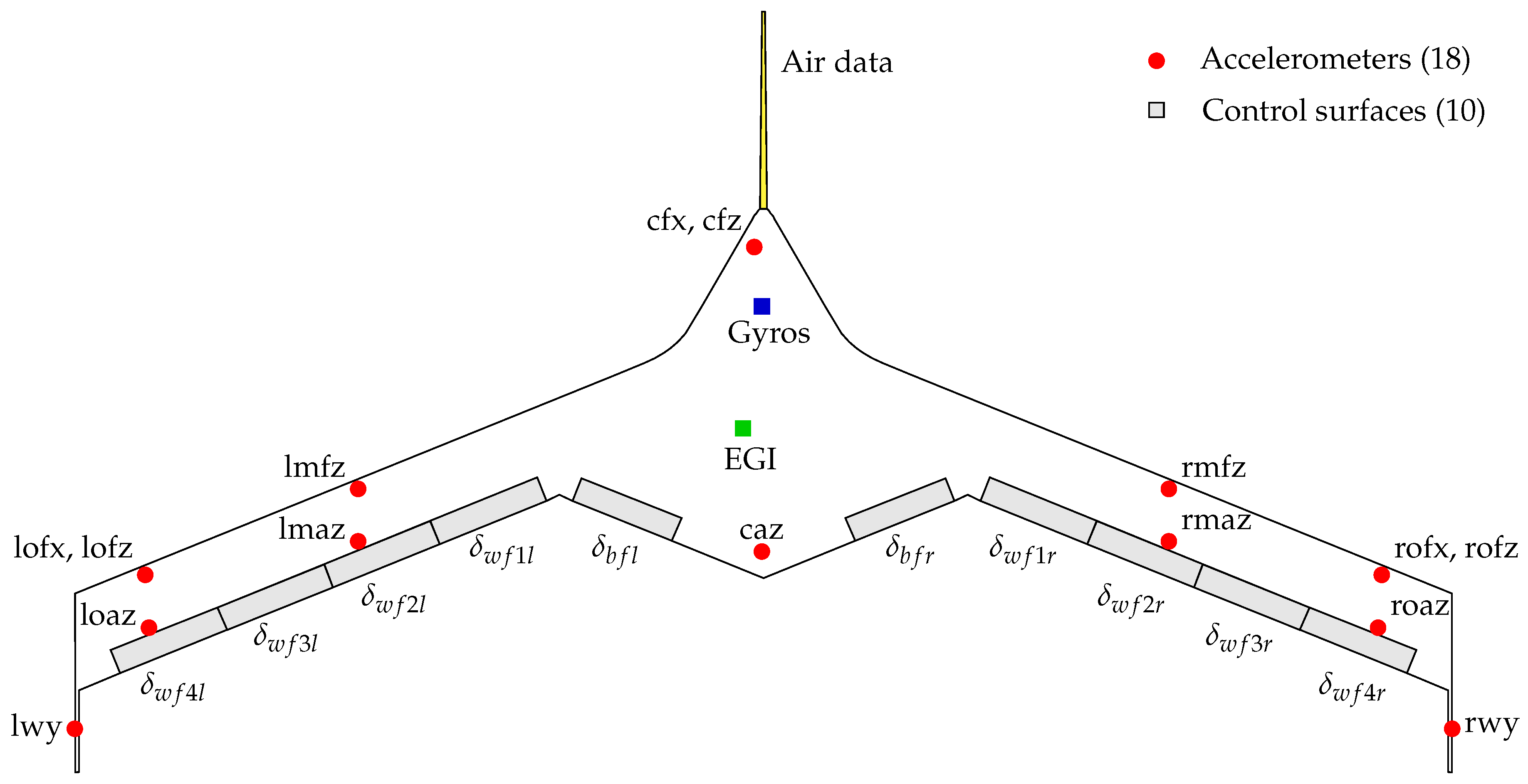
Figure 4 over the same time duration. Many other output measurements were available but were not used in this analysis to keep the parameter estimation problem smaller. In addition, measurements from accelerometers on the left and right wings were averaged to reduce the number of outputs, for example as
similar to the control surface deflections. At the start of the data record, the aircraft was approximately in straight and level flight. There was some motion of the aircraft due to setting up the flight condition, dynamic coupling of the system, and light turbulence. The variations in the response measurements after the onset of the multisine excitations were small and not much bigger than before the onset, but nonetheless produced good data for modeling due to the high-quality sensors used. Spectral analysis showed that the apparent high levels of noise in the accelerometers installed in the center body and wing (for example,
) relative to
were instead due to the presence of many high-frequency structural modes in the data. Variations in the other flight variables were very small, for example a 1.2% variation in airspeed, 0.3% change in altitude, 0.4% change in mass resulting from a 5.5% decrease in fuel, and 0.1% change in pitching moment of inertia. The average fuel weight condition for this maneuver was 32% and the average airspeed was about 80% of the flutter speed.
Measured input and output data were transformed into the frequency domain at the harmonic frequencies in the multisine inputs. Using only these frequencies in the transforms reduced the computational complexity for the optimization. Estimation results did not significantly change when additional frequencies were used since the input power was concentrated in these frequencies; however, the amount of computation time needed to run the output-error analysis substantially increased.
Simple methods were used to estimate scale factor errors in the angle of attack and pitch angle data, as well as time skews for all measurement Fourier transforms relative to the accelerometer data [
11,
29]. The Fourier transform data were then corrected for these errors. Because there is no kinematic redundancy between the control surface deflections and output responses, a delay for the input
was added to Equation (
22) as
to account for the time skew between the input and output measurement data buses. The input time skew was estimated at the same time as the stability and control derivatives (described next) and did not exhibit any correlation issues. Overall, this process was a simple and effective way for synchronizing the data and enforcing consistency of the response measurements which improved the data quality. Although time skew and scale factor errors were small, they affected the parameter estimation results. In particular, the stability and control derivatives pertaining to the structural modes were sensitive to the time delay values.
Once the data were corrected for time skews and scale factor errors, output error parameter estimation was applied to determine estimates of the non-dimensional stability and control derivatives and the input time skew. Starting values for the model parameters in the nonlinear optimization were obtained from an aeroelastic panel code model of the X-56A using finite differences. The model structure (the subset of possible stability and control derivatives that can be accurately estimated using the data) was adjusted using trial and error until the parameter estimates seemed adequate, standard errors were reduced, fits to data were close, and the estimator converged quickly. This process was tedious and time consuming, but previous experience with this aircraft, insight using other analyses [
17,
18], modifications to the output-error code to increase flexibility in choosing the model structure, and reduction of the output-error optimization problem helped.
For this analysis, structural parameters such as the mode shapes and in-vacuo frequencies were substituted from the FEM and only non-dimensional stability and control derivatives and the input time skew were estimated. If structural parameters were not available, as in many flight tests, they could also be estimated from the flight data. However, only the equivalent structural damping and frequency (for example, the combined or terms) could be identified in this case and maneuvers at different dynamic pressures would be required to separate the air-off and air-on contributions. Similarly, the mode shapes (for example, ) could be identified, up to a scale factor, but these identified values would pertain to the air-on mode shapes and not correspond to the in-vacuo modes used as basis shapes to parameterize the structural deformations. Having accurate estimates of the structural parameters therefore allows more insight into physical parameters and creates a model with a larger range of applicability.
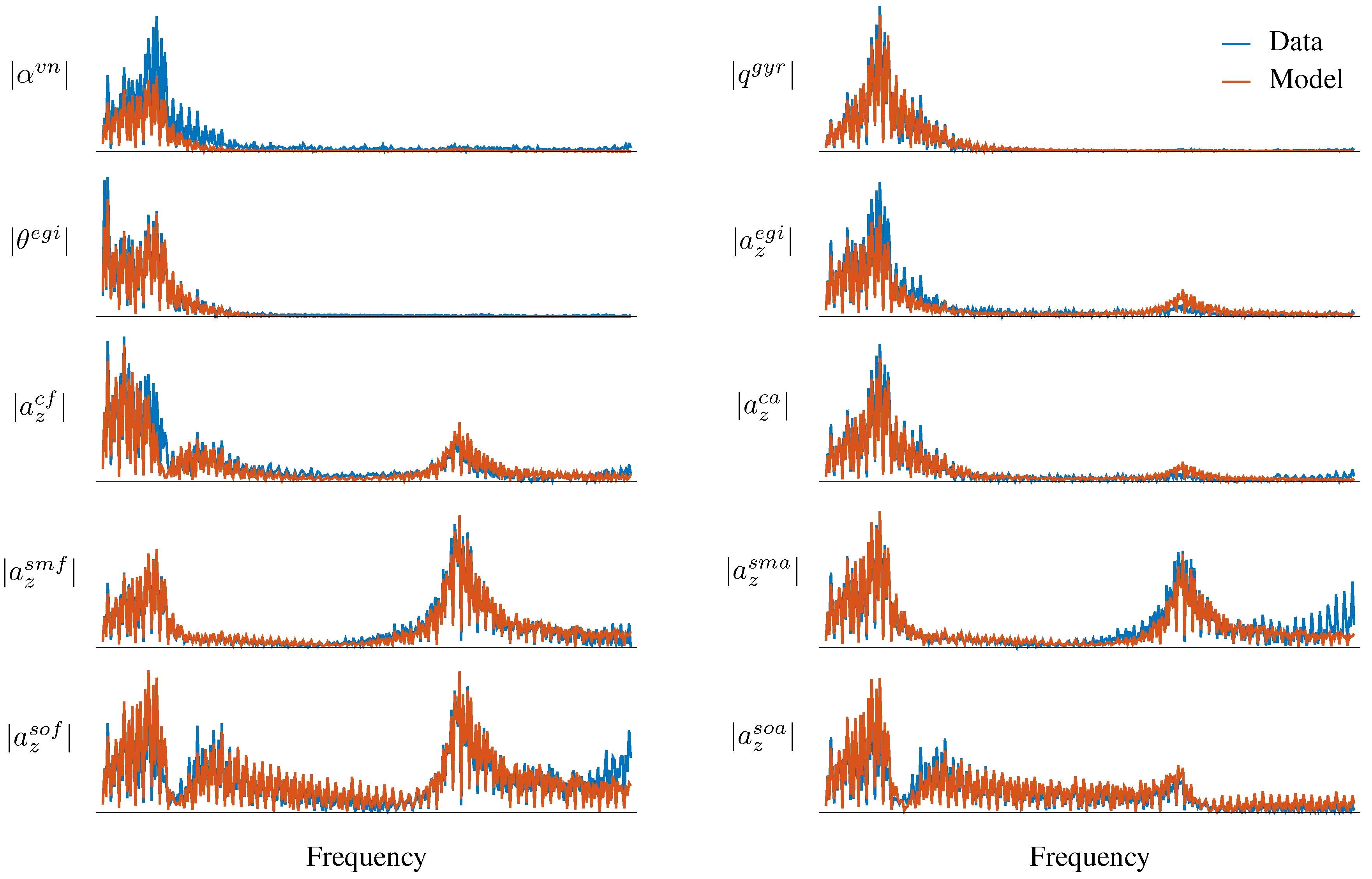
Fits of the model outputs to measured output data are shown in
Figure 6. The x-axes span the bandwidth of the excitation, whereas all the y-axes have different ranges. The short period, SW1B, and SW1T modes are clearly present in the data. There was some excitation of the SWL mode in the higher frequencies. The SFA mode did not have much participation in these output measurements. Overall, the model outputs fit the data well over the entire excitation bandwidth. There was some mismatch at low frequencies near the short period mode in
,
, and
and at higher frequencies in
and
. These errors could be due to low-frequency coupling with neglected structural dynamics, unsteady aerodynamics, or other factors. The low-frequency mismatches could also be due in part to errors in the assumed displacement mode shapes of the structure at these sensors obtained from the FEM. However, in general these were good fits to the data and the estimator converged quickly from the starting values.
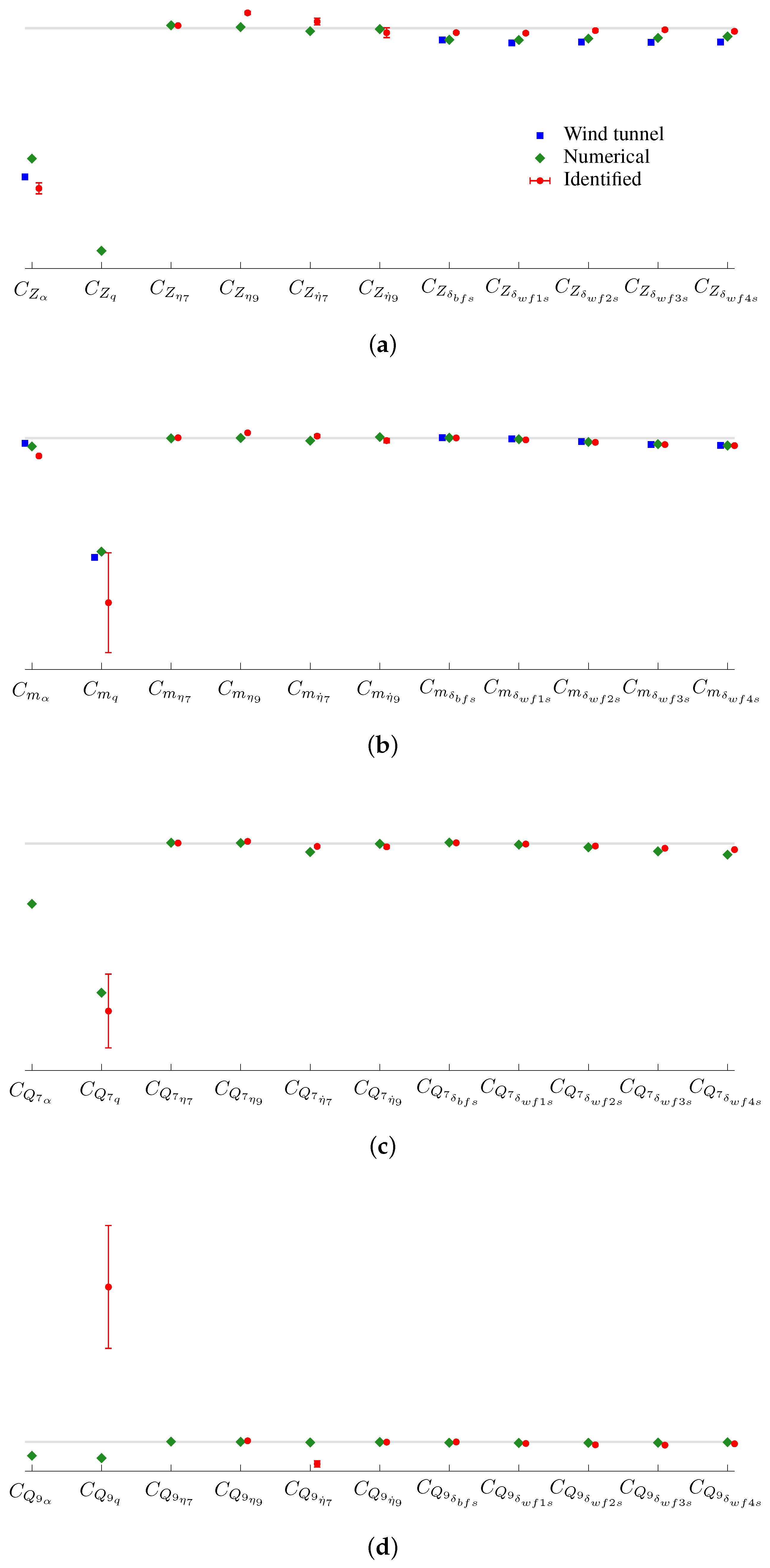
Estimates of non-dimensional stability and control derivatives are shown in
Figure 7. Markers in blue squares were from a static wind tunnel test using a scaled half-span model of the X-56A. Prior estimates were not available for the angular rate derivatives or aeroelastic derivatives from these sources. Estimates shown as green diamond markers were obtained from the aeroelastic panel code model of the X-56A in the 50% fuel configuration using finite differences. Estimates identified using output error in the frequency domain are shown as red circles, where the error bounds indicate the estimated
standard errors. The parameters
,
,
, and
were not statistically significant, as indicated by the size of their standard errors, and were removed from the model structure. The other parameters, in general, had moderate agreement with the other predictions and had adequate standard error levels. The control derivatives were very close to the predicted values. The angle of attack derivatives had good agreement. The pitch rate derivatives exhibited larger amounts of variation between the estimates. These derivatives are weaker and are typically more difficult to estimate. Improvements could be made with a more refined data compatibility analysis and by installing additional high-rate gyroscopes in the aircraft.
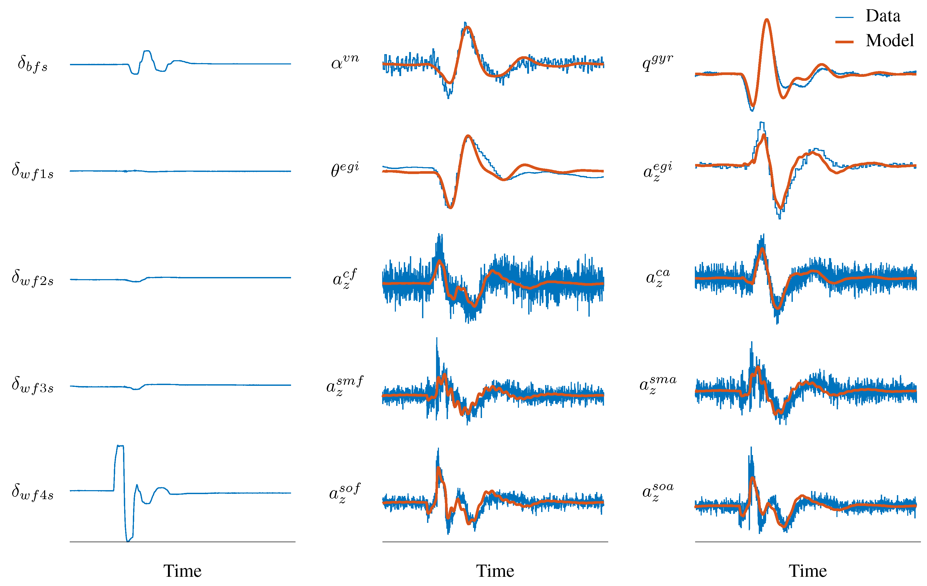
A second maneuver was used to test the predictive capability of the model. The validation maneuver, data for which are shown in
Figure 8, involved a different type of excitation input and was conducted during a subsequent flight at a different altitude and weight. The average fuel weight for the validation maneuver was 64%, which was heavier than 32% used in the identification case and changed the aeroelastic properties of the airplane. The first column of plots in
Figure 8 shows the control surface deflections. A doublet was performed on the
surface targeting the SW1B mode, although the short period and SW1T responses are also present in the response data. A control system was running and some feedback is present in the control surface deflections. The measured output responses are shown in blue in the second and third columns. The red time histories are the outputs of the identified linear model, driven using the measured control surface deflections. Although there are some differences between the model outputs and the measurements, the output of the model was in general close to the measured flight test data, thereby validating that the identified model captures the salient features of the response. The availability of FEM/GVT structural data and the identification of non-dimensional aeroelastic derivatives facilitated using a validation maneuver from a different flight condition than that used for identification.
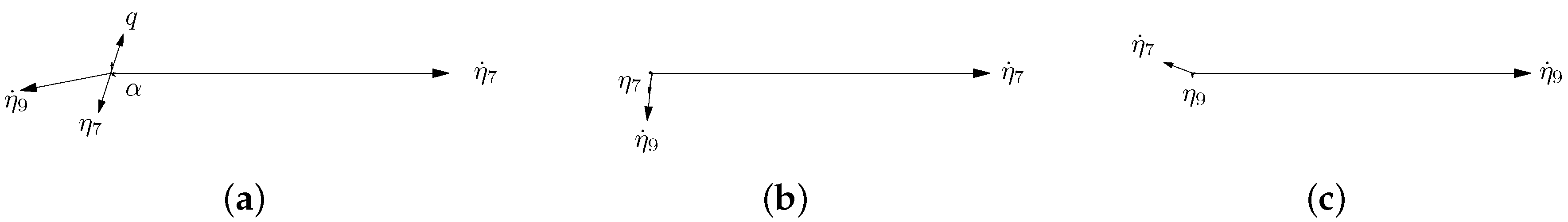
Figure 9 shows eigenvector phasor diagrams for the identified model. Drawn in polar coordinates, these diagrams illustrate how much and with what phasing each state participates in the modal response. Although each mode contains contributions from all states, only the most significant states are noted in these diagrams. Eigenvectors associated with the structural modes are still referred to as SW1B and SW1T here, although these are similar to but technically different from the in-vacuo vibration modes due to the aerodynamic interactions [
5].
Figure 9a is the elastic short period mode. The normal phasing between
and
q is present, but the elastic states
,
, and
play a large role in the modal response and indicate the large degree of flexibility in this aircraft. Note that the states
and
q in these phasor diagrams are different than the outputs
and
defined in Equations (
17) and (
18). For the SW1B mode shown in
Figure 9b, the response is mainly due to
with smaller contributions due to
and
. Similarly, for the SW1T mode shown in
Figure 9c, the response is mainly due to
with smaller contributions due to
and
.
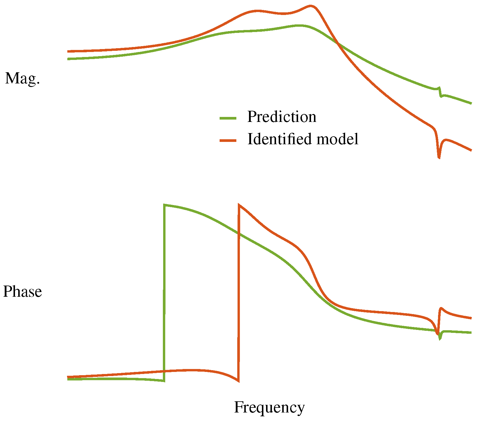
Bode plots showing the frequency responses from the
input to the measured pitch rate at the gyroscope
are shown in
Figure 10. The frequency response using the aeroelastic panel code, truncated to include only the short period, SW1B, and SW1T modes, is shown in green, whereas the identified model is shown in red. The frequency response for the identified model is similar to the aeroelastic panel code prediction, but has larger magnitudes near the short period and SW1B modes. The faster roll-off of the model after the SW1B mode exhibited in the identified response was corroborated by a separate analysis using frequency responses [
18].
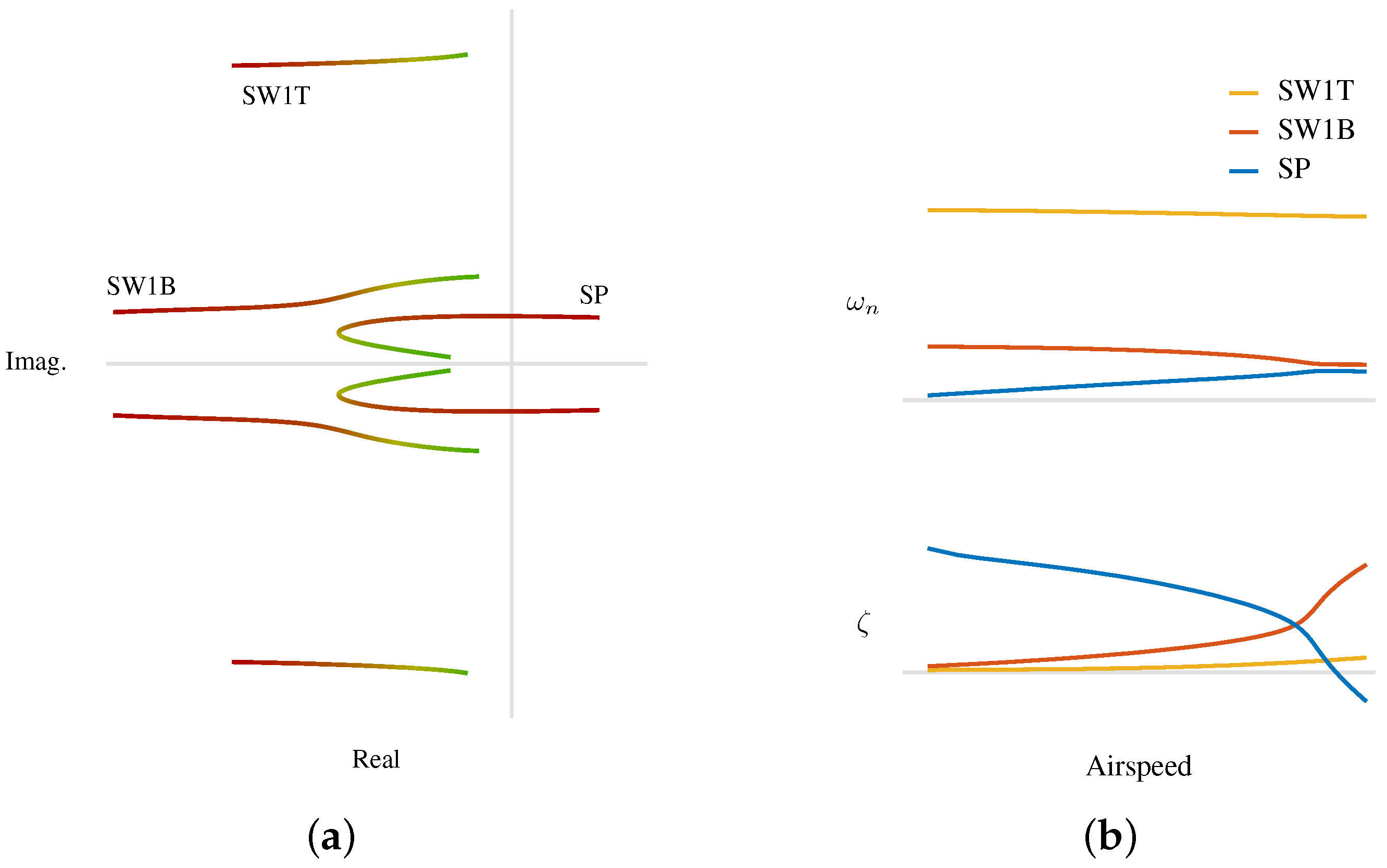
Figure 11 shows variation in the modal characteristics of the identified model as airspeed and dynamic pressure are increased. In
Figure 11a, the dynamic-pressure root locus shows the migration of eigenvalues in the complex plane as dynamic pressure increases from about 15% of the flutter speed (green) to about 115% of the flutter speed, with all other model parameters (such as altitude, fuel weight, etc.) held constant. Again, SW1B and SW1T refer to the aeroelastic modes, which are technically different than the genesis vibration modes obtained when
. In
Figure 11b, the frequency and damping ratio of the eigenvalues are shown as airspeed increases over the same range. These plots indicate that as the X-56A flies faster, the aeroelastic SW1B and SW1T modes decrease slightly in frequency and increase in damping ratio, remaining stable, whereas the short period mode increases in frequency and decreases in damping ratio, becoming unstable. It was expected from other numerical modeling predictions that the short period and SW1B would coalesce at higher dynamic pressures; however, the SW1B mode was expected to become unstable, rather than the short period mode. Recent flight tests at airspeeds near and beyond the flutter speed have corroborated that the short period mode becomes unstable, as shown in
Figure 11a.
7. Conclusions
In this paper, the identification of aeroelastic models for the X-56A airplane longitudinal dynamics from flight test data is discussed. The excitations for the maneuver were orthogonal phase-optimized multisine inputs, which perturbed control surface pairs at the same time but in different ways while a feedback control system was active. The Waszak–Schmidt aeroelastic flight dynamics model, an extension of traditional flight dynamics models using quasi-steady stability and control derivatives, was used for identification. Parameter estimation was performed using the output-error approach to match Fourier transforms of measured output response data. A validation maneuver was used to demonstrate the predictive capability of the identified model under different conditions, and modal characteristics of the identified model were explored. Practical aspects of the experiment design and system identification analysis for flexible aircraft are discussed throughout the paper.
The main findings of this paper can be summarized as follows:
Orthogonal phase-optimized multisines are effective inputs for efficiently exciting aeroelastic aircraft with multiple control effectors using a specified frequency bandwidth and power spectra for system identification.
Application of output error parameter estimation to determine non-dimensional stability and control derivatives that best match model outputs to Fourier transforms of measured output data was a successful approach for identifying an aeroelastic model of the X-56A from flight test data.
The Waszak–Schmidt aeroelastic flight dynamics model was useful for system identification and was a good representation of the observed flight dynamics at different airspeeds and fuel weights.
The orthogonal phase-optimized multisine inputs proved a good input for exciting the X-56A aircraft for aeroelastic identification. The inputs were run simultaneously on multiple control surfaces, which facilitated the identification of the entire model from a single maneuver with a relatively short time duration. Although a control system was running, control surface deflections exhibited low pair-wise correlations and were of good quality for modeling. Arbitrary design of the excitation bandwidth and power spectra facilitated targeting of specific modal responses in the output data for modeling.
The estimation of model parameters using output error to match Fourier transforms of measured response data had several advantages. Output error is based on maximum likelihood estimation, which gives a theoretical justification to the estimated parameters and uncertainties. Furthermore, it includes relevant simplifications and can incorporate a large amount of data measured from multiple sensors. Analysis using frequency-domain data reduces the number of data points to process and the number of unknown model parameters to estimate, and makes it computationally more efficient to solve the equations of motion for each iteration of the optimization. In general, the frequency-domain approach also illuminates modal responses, which are separated in frequency.
Drawbacks of the estimation approach are that the analysis is restricted to linear models, iterations are needed in the optimization from good starting values for the model parameters, and changes to the model structure can be cumbersome to implement. The results of this identification were intended for analysis and control design, and the maneuver involved small perturbations about a reference condition, so linear models were adequate for the identification. Starting values were obtained from a separate analysis using an aeroelastic panel code model. Convergence of the estimator was attained relatively quickly by simplifying the estimation problem and using frequency-domain data. Determining model structure, however, was tedious and time-consuming using this approach due to the large number of possible model parameters. Recent work with the X-56A using the equation-error approach, where statistical metrics can be applied to automatically select the aerodynamic model structure, and using frequency responses, where the model structure can be inferred from Bode plots, was leveraged in choosing the aeroelastic derivatives to estimate.
The Waszak–Schmidt aeroelastic flight dynamics model was an appropriate choice for system identification using the X-56A airplane. The model structure was relatively simple but able to capture the effects of aeroelasticity, including flutter, and was based on the familiar quasi-steady stability and control derivatives traditionally used for flight dynamics models. Because in-vacuo vibration modes parameterized the structural deformations and because data from a finite element model and ground vibration test were available, non-dimensional aeroelastic stability and control derivatives were identified. This allowed a single set of coefficients, obtained below flutter speeds, to predict aircraft dynamic behavior at higher speeds including the aeroelastic instability observed in flight.
Overall, the approach presented in this paper was an efficient, effective, and successful method for identifying aeroelastic flight dynamics models from measured flight test data. The results are representative of flight in several conditions, including those that result in aeroelastic instabilities such as flutter. The models identified can be used to refine simulation models and to design feedback control laws such as for active flutter suppression or gust load alleviation.


