Article

Path Planning Using Concatenated Analytically-Defined Trajectories for Quadrotor UAVs †

Mechanical and Aerospace Engineering, University of Strathclyde, 75 Montrose Street, Glasgow G1 lXJ, UK
*
Author to whom correspondence should be addressed.
This paper is an extended version of our paper published in ECC 15, Linz, Austria.
Aerospace 2015, 2(2), 155-170; https://doi.org/10.3390/aerospace2020155
Submission received: 23 February 2015 / Revised: 26 March 2015 / Accepted: 16 April 2015 / Published: 21 April 2015
(This article belongs to the Special Issue Unmanned Aerial Systems 2015)

Abstract

:
This paper presents a semi-analytical trajectory planning method for quadrotor UAVs. These trajectories are analytically defined, are constant in speed and sub-optimal with respect to a weighted quadratic cost function of the translational and angular velocities. A technique for concatenating the trajectories into multi-segment paths is demonstrated. These paths are smooth to the first derivative of the translational position and pass through defined waypoints. A method for detecting potential collisions by discretizing the path into a coarse mesh before using a numerical optimiser to determine the point of the path closest to the obstacle is presented. This hybrid method reduces the computation time when compared to discretizing the trajectory into a fine mesh and calculating the minimum distance. A tracking controller is defined and used to show that the paths are dynamically feasible and the typical magnitudes of the controller inputs required to fly them.

Graphical Abstract

1. Introduction

Unmanned aerial system (UAS) applications often require the vehicle to fly in areas with many obstacles. With this desire to fly in restricted space, such as urban environments, there is increasing need for better path and trajectory planning. Typical UAS civilian applications, such as data collection, environmental monitoring and security, require autonomous navigation to avoid collisions without the assistance of a pilot.
There are a variety of different UAS types, including fixed-wing planes, helicopters and multi-rotors. For agile navigation in small areas with tight space constraints or a dense field of obstacles, quadrotors are most suitable. Their ability to hover in a stationary position is also beneficial when awaiting instructions or collecting data using on-board sensors. In contrast, fixed-wing vehicles can efficiently cover greater distances and have faster maximum speeds. However, they cannot hover (barring experimental vehicles, such as [1]), which limits their use in certain scenarios. Additionally, their dynamic constraints restrict their manoeuvrability, and they must maintain a minimum airspeed to produce sufficient lift. Finally, helicopters offer similar performance and agility to multi-rotors, but their mechanical complexity is not justified at the scale of standard UAS. This paper will focus on trajectory generation for multi-rotors (specifically, quadrotors), because they have the least dynamic constraints; however, future work will investigate applying an extension of the methods to other vehicles.
The differential flatness of quadrotor dynamics can be exploited to allow for easier planning using the decoupled translational axes [2]. A yaw angle also needs to be defined; in the literature, this is normally fixed at zero. One technique for trajectory planning is to use an analytical function to describe the position over time. The shape of the function is altered by varying parameters. After defining an error function for the final state, a numerical minimization is performed to calculate the parameters that satisfy the boundary conditions. The derivatives of the state can be found by differentiating the analytical function. Functions that have already been used for quadrotor trajectory planning include splines [3], polynomials [4] and Bézier curves [5]. In this paper, we use the maximum principle of optimal control to define curves using standard functions that are sub-optimal with respect to a weighted quadratic cost function. The term sub-optimal is used as the analytical curves are the projection of optimal curves on S E ( 3 ) onto R 3 , and the rotational component of the optimal motion is not used in the motion planning.
A typical method of defining obstacles is to use p-norms [6] and is applicable in both two- and three-dimensional planning. This method can also be extended to polygonal shapes [7]. However, for the purpose of demonstrating the obstacle detection algorithm, the obstacles in this paper are defined as spheres. Obstacle avoidance using Dubins curves and sampling-based planning is considered in [8]. Methods for avoiding other moving vehicles and obstacles are given in [9,10].
This paper extends our conference paper [11] to develop concatenation of trajectories to form multi-segment paths and the obstacle detection algorithm. The format of this papers is as follows. The quadrotor dynamics and kinematics are presented in Section 2, with the analytical function defining the curves given in Section 3.1. The method for repositioning the generated curves is described in Section 3.2, and forming a single path from curves patched together is demonstrated in Section 5.2. An obstacle detection algorithm is presented in Section 4 and evaluated in Section 5.3. A tracking controller is defined (Section 5.1) and used to demonstrate the feasibility of the path in Section 5.2. Finally, the findings are summarised and future work discussed in Section 6.

2. Quadrotor Dynamics and Kinematics

A standard quadrotor has four motors and propellers arranged in a square formation. It has an inertial translational position, velocity and acceleration x = [ x 1 , x 2 , x 3 ] T , x ˙ = [ x ˙ 1 , x ˙ 2 , x ˙ 3 ] T and x ¨ = [ x ¨ 1 , x ¨ 2 , x ¨ 3 ] T , respectively. The angular velocities about the body axes are Ω = [ Ω 1 , Ω 2 , Ω 3 ] T , and the body frame velocities are v = [ v 1 , v 2 , v 3 ] T . The forces generated by the propellers are f = [ f 1 , f 2 , f 3 , f 4 ] T , and the moments induced in the body-fixed frame are denoted as M = [ M 1 , M 2 , M 3 ] T . The total thrust is defined as F = i = 1 4 f i . The mass of the quadrotor is denoted by m and the inertia matrix by J R 3 × 3 . The body-frame thrust vector is e 3 = [ 0 , 0 , 1 ] T . In matrix form, the total thrust and moments are:
F M 1 M 2 M 3 = 1 1 1 1 0 d 0 d d 0 d 0 c τ f c τ f c τ f c τ f f 1 f 2 f 3 f 4
where d is the distance between the centre of the quadrotor and c τ f is a constant that relates thrust to induced yaw. In this paper, the quadrotor is treated as a rigid body with a constant gravitational acceleration g a . To simplify the procedure of the motion planning and controller design, typical aerodynamic disturbances on the moments and forces, such as drag, ground effect and rotor dynamics, are neglected. The simulated quadrotor dynamics follow the derivations in [12,13,14]. The equations of motion are as described in [15]:
x ˙ = R v
m x ¨ = m g a e 3 F R e 3
R ˙ = R Ω ^
J Ω ˙ + Ω × J Ω = M
with R S O ( 3 ) , where:
SO ( 3 ) = Δ { R R 3 × 3 : R T R = I and det ( R ) = 1 }

3. Trajectory Planning

The first subsection defines the curves and the basis behind them. The second demonstrates the process to reposition the curves from starting at the origin to a specified translational position and orientation in the inertial frame.

3.1. Sub-Riemannian Curves for Quadrotor Trajectory Planning

The kinematics, Equations (2) and (4), can be expressed equivalently on the Euclidean group of motions S E ( 3 ) :
d g d t = g ( n = 1 3 B i v i + n = 1 3 A i Ω i )
where A 1 , A 2 , A 3 , B 1 , B 2 and B 3 are the basis elements of the Lie algebra of the Lie group S E ( 3 ) [16,17,18,19] with g S E ( 3 ) :
g = 1 0 0 0 x R
Body velocities for the planned motion were specified as v 1 = v 2 = Ω 3 = 0 to simplify the process of deriving analytical expressions for the reference curves. It is convenient to choose a single translational body velocity, so that the translational speed in the inertial frame is equal to the magnitude of that body velocity. The translational speed will also be constant, since after applying the maximum principle, it is shown that the translational body velocity is time invariant. Additionally, having a single non-zero body velocity facilitates the joining of trajectory segments using the method described in Section 3.2. Future work will consider the inclusion of the other body velocities. With the given restrictions on the body velocities, Equation (7) can be reduced to:
d g d t = g ( v 3 B 3 + A 1 Ω 1 + A 2 Ω 2 )
We choose to define a set of curves for motion planning that minimizes the cost function:
J = 1 2 0 T v 3 2 + c ( Ω 1 2 + Ω 2 2 ) d t
subject to the nonholonomic constraint Equation (9) and given boundary conditions g ( 0 ) = g 0 and g ( T ) = g T , where c is a constant weight and v i and Ω i are measurable and bounded functions. A curve that satisfies the constraint Equation (9) and minimizes the cost function subject to the boundary conditions defines a sub-Riemannian curve on S E ( 3 ) [19].
Sub-Riemannian curves are useful for trajectory planning, because they are smooth and globally defined on S E ( 3 ) , unlike Euler angles or quaternions that use local co-ordinates. They also naturally satisfy the constraint Equation (6). In this particular case, they can also be analytically defined, which reduces the motion planning problem to one of parameter optimisation. The full derivation for the curves is presented in Appendix. The curves are defined using standard functions; knowledge and understanding of their derivation are not required for their application. They are obtained by a projection of a particular sub-Riemannian curve g p S E ( 3 ) onto x p R 3 , where x p = [ x p 1 , x p 2 , x p 3 ] T and:
x p 1 = c 2 ν γ ( 1 cos γ t sin β + c 1 cos β sin γ t γ t ) x p 2 = c 2 ν γ ( 1 cos γ t cos β c 1 sin β sin γ t γ t ) x p 3 = c 2 2 ν γ sin γ t + c 1 2 ν t
where:
s = λ 1 2 + λ 2 2 λ 3 = λ 4 λ 1 λ 2 r = λ 3 2 + λ 4 2 β = a t a n 2 ( λ 2 , λ 1 ) c 1 = ν r 2 + ν 2 c 2 = r r 2 + ν 2 γ = s r 2 + ν 2 r c
The quadrotor speed ν and weighting c are chosen by the user before the optimisation. A desired final position x d = [ x d 1 , x d 2 , x d 3 ] T is also specified by the user. A numerical optimisation using MATLAB’s f m i n c o n that implements a sequential quadratic programming method with an active-set region was used to find the optimisation vector Ξ = [ λ 1 , λ 2 , λ 4 , T ] that minimizes the error in the final position:
C x f = ( x d ( T ) x p ( T ) ) 2
where T is the final time and constrained such that T > 0 . The translational velocity x ˙ p can be defined analytically by taking the first derivative of Equation (11):
x ˙ p 1 = c 2 ν ( c 1 cos β cos γ t 1 + sin β sin γ t ) x ˙ p 2 = c 2 ν ( c 1 sin β 1 cos γ t + cos β sin γ t ) x ˙ p 3 = ν ( c 1 2 + c 2 2 cos γ t )
Likewise, the second derivative of Equation (11) gives the translational acceleration:
x ¨ p 1 = c 2 ν ( γ cos t γ sin β c 1 γ cos β sin t γ ) x ¨ p 2 = c 2 ν ( γ cos t γ cos β + c 1 γ sin β sin t γ ) x ¨ p 3 = c 2 2 ν γ sin t γ
The magnitude of the acceleration is:
a = x ¨ p 1 2 + x ¨ p 2 2 + x ¨ p 3 2
It can be shown that a is constant by substituting Equation (15) into Equation (16) and simplifying:
a = a b s c 2 ν γ
The magnitude of the velocity is constant and simply ν, as determined by the user before calculating the optimisation vector.

3.2. Trajectory Repositioning and Reorientation

For the particular curves described in Section 3.1, the initial position and rotation are, respectively:
x p ( 0 ) = [ 0 , 0 , 0 ] T R ( 0 ) = I
where I is the the identity matrix. The curves can be placed anywhere in the inertial frame x i ( t ) using:
[ 1 x i ( t ) ] T = g i ( 0 ) . [ 1 x p ( t ) ] T
where g i ( 0 ) is the initial state of the path. It should be noted that g i ( t ) includes a description of the rotation (R) of the curve over time. However, this is not used as part of the trajectory tracking, because it is purely kinematic and does not account for the dynamics (such as gravitational acceleration). Similarly, for an initial and desired state in the inertial frame, the final state g p ( T ) for the particular curves is given by:
g p ( T ) = g i ( 0 ) 1 . g i ( T )
Since the final rotation is not used when generating the curves using the numerical optimiser, the translation position x p ( T ) can be retrieved from:
[ 1 x p ( T ) ] T = g p ( T ) . [ 1 0 0 0 ] T
The paths generated using this procedure of joining trajectories are smooth to the second derivative; there are no discontinuities in position or velocity. However, they are not smooth in the third derivative, because the trajectories have different curvatures, so it is not possible to match acceleration.

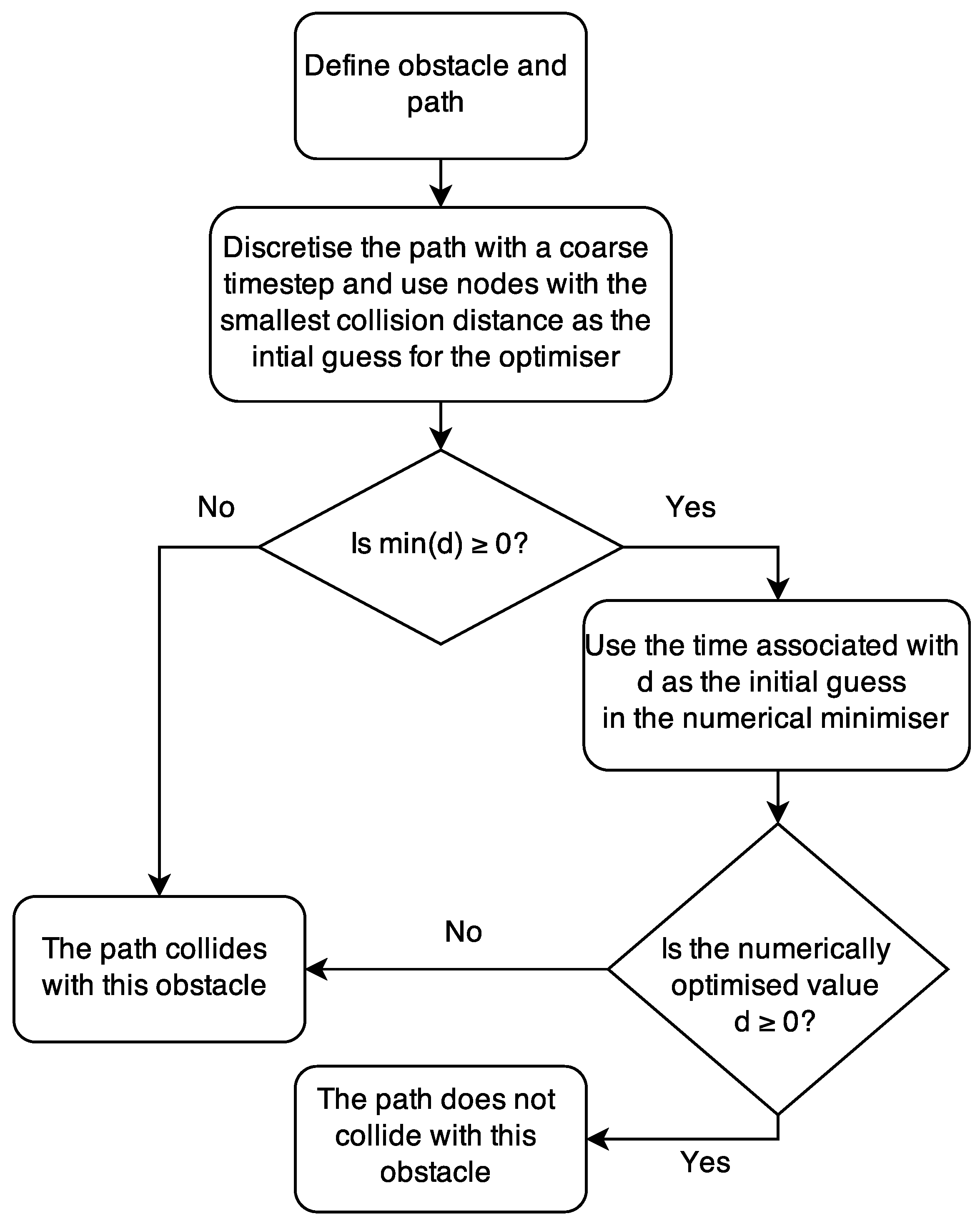
4. Obstacle Detection

A simple method for checking the validity of a path in the obstacle space is to discretize it into nodes separated by a small time step. Each node lies on the path and can be checked for collisions. The choice of time step is a trade-off between computational time and the completeness of the check. This method can be extended to a hybrid method using a large time step and then performs a numerical minimization to find the smallest collision distance d along the path. The collision distance for an obstacle is defined as the Euclidean distance between the edge of the object and the quadrotor:
d ( t ) = x o b s x i ( t ) r o b
where x o b s R 3 is the centre of the sphere, x i is the planned translation position of the quadrotor Equation (19) using the curves described in Section 3.1 and r o b is the radius of the sphere. For practical purposes, some additional margin should be given, because the actual size of the quadrotor is not accounted for by Equation (22).
The paths are composed of trajectories patched together using the method explained in Section 3.2. To find the location on a path where an object is closest, the optimisation vector for the relevant segment must be loaded. The concatenated nature of the path is not an issue, because there are no discontinuities in position when transitioning between trajectories. Time was constrained, such that:
0 t T
and the function to minimize is:
d m i n = m i n d ( t )
where d m i n is the minimum collision distance along a path for a specified object. If d m i n 0 , then the quadrotor will not collide with the obstacle, providing that the tracking controller guides the vehicle along the planned trajectory.
The simple local optimiser ( f m i n c o n ) used in this paper has the potential to get caught in local minima. A global optimiser may be more suitable (such as a genetic algorithm [20]), but the trade-off between computational expense and accuracy needs to be investigated in more detail. However, in this paper, we demonstrate the implementation of the general analytical method by using the local optimiser and by providing a suitable initial guess. The hybrid method used in this paper combines discretization with a large time step and then uses a numerical minimizer to determine the precise location and magnitude of the collision distance. If any of the points are d ( t ) < 0 , then the algorithm terminates and the path is reported as invalid. The process of the hybrid algorithm is represented pictorially in Figure 1. An evaluation of the collision detection algorithm is performed in Section 5.3 and compared to discretizing the trajectory with a small time step.
Figure 1. Obstacle detection algorithm.
Aerospace 02 00155 g001

5. Simulations

In the first of the following subsections, the tracking controller is described that is used to simulate the path generated in Section 5.2. Finally, Section 5.3 tests the hybrid obstacle detection algorithm and compares it to discretizing with a coarse time step.

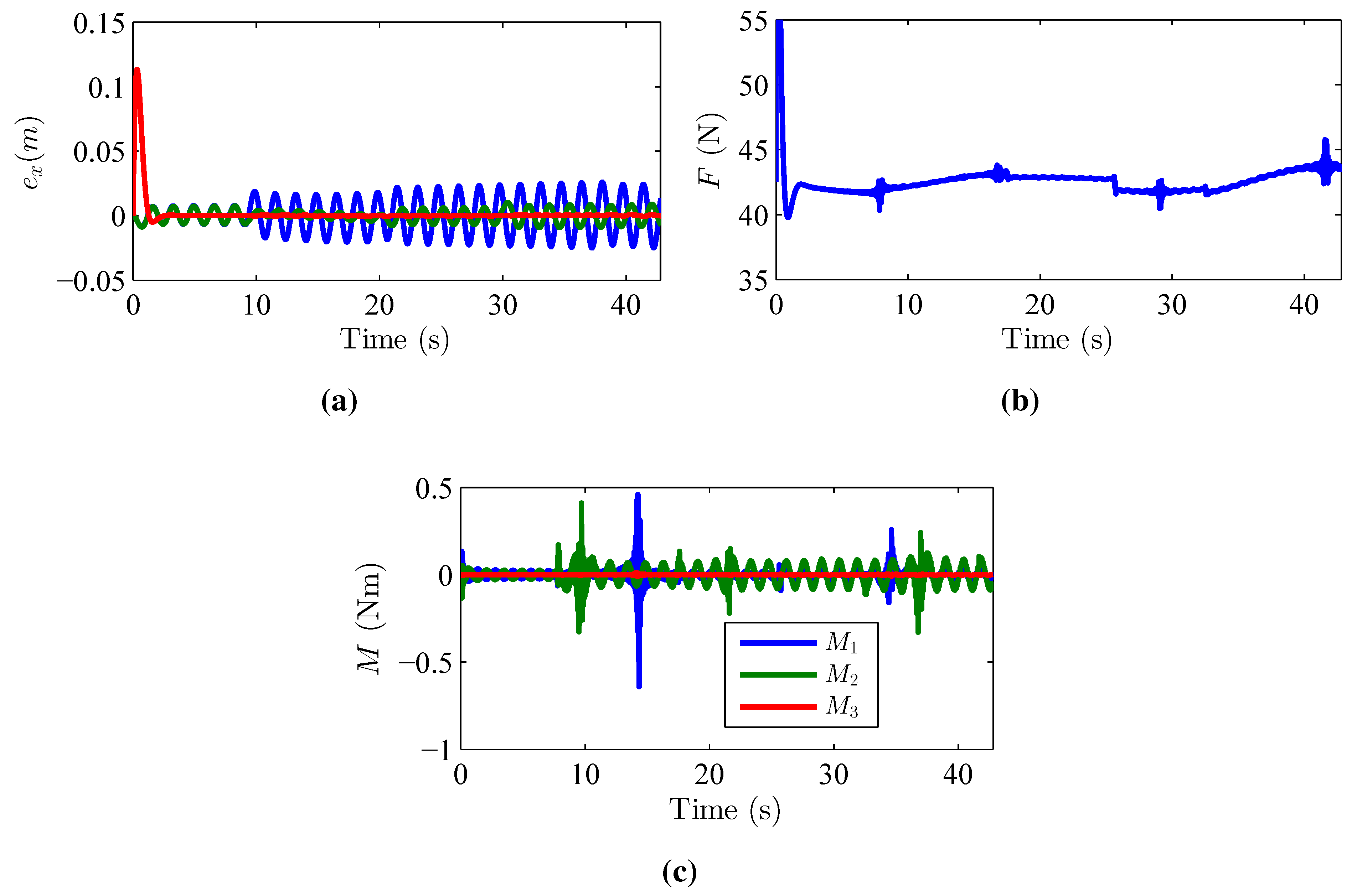
5.1. Tracking Controller
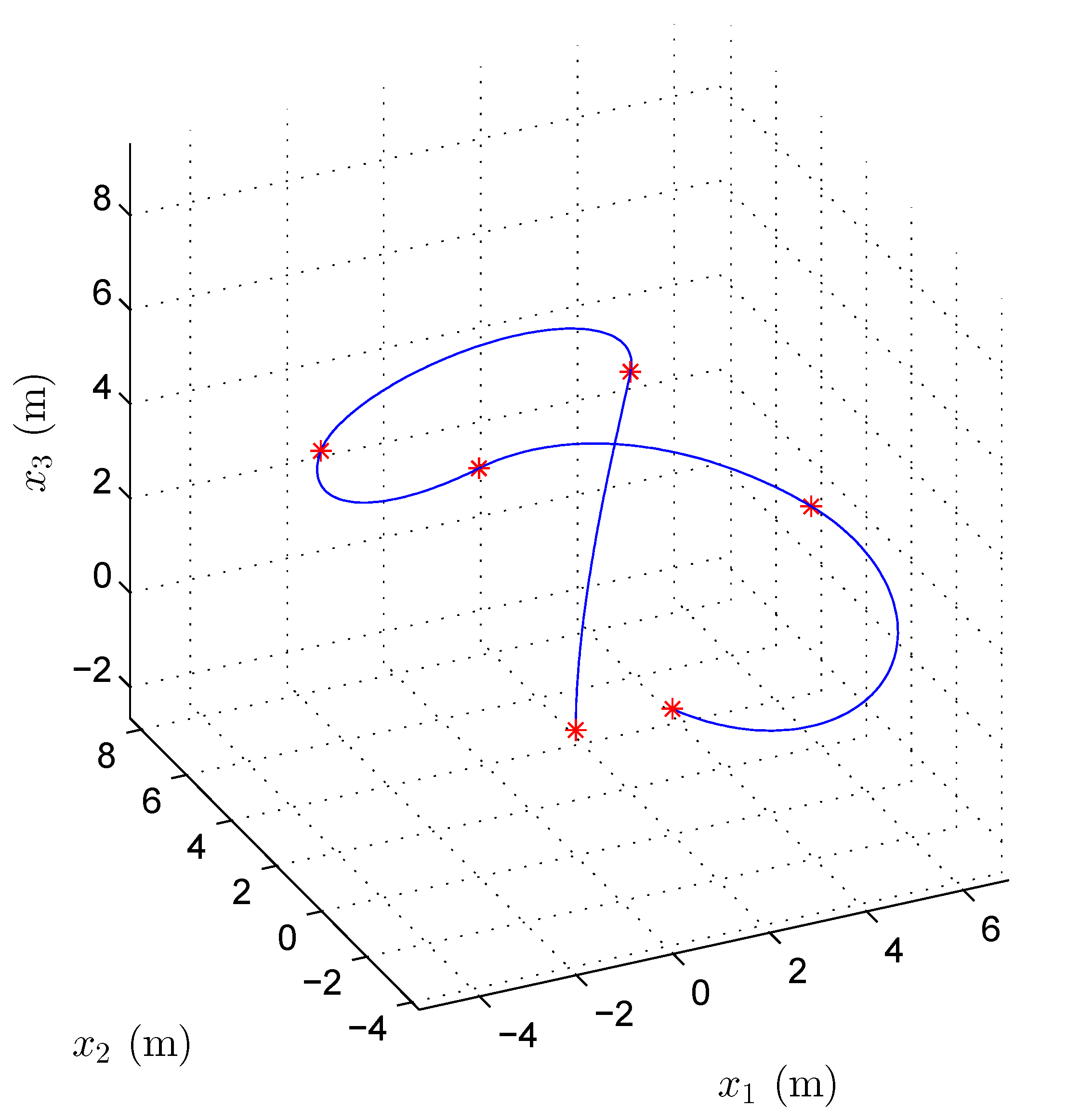
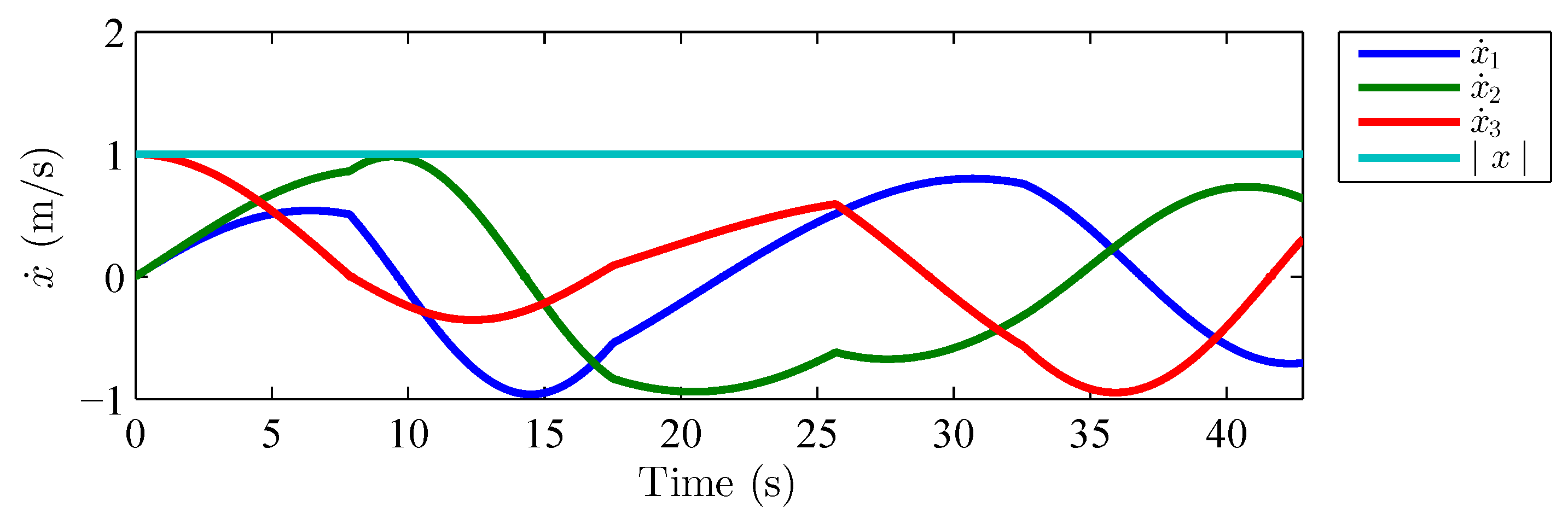
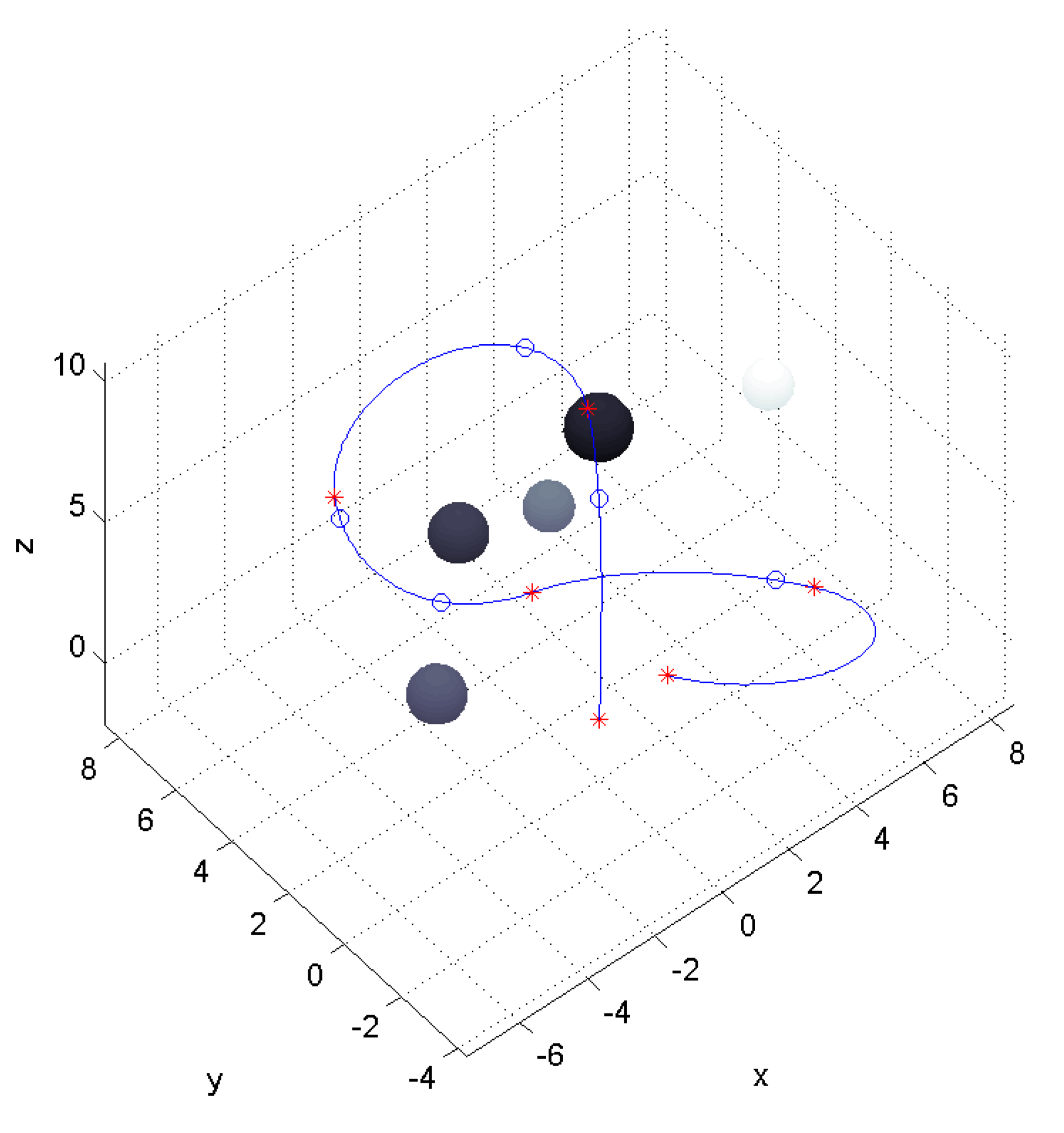
The tracking controller was used in this paper to demonstrate the feasibility of the trajectories and was first presented in [15]. In addition to the favourable tracking performance, this controller was chosen because the trajectories are generated on the S E ( 3 ) group. The tracking errors for position, velocity and angular velocity are defined as:
e x = x x p
e v = x ˙ x ˙ p
e Ω = Ω R T R d Ω d
where Ω d = R d T R d ˙ , and the desired rotation is defined as:
R d = [ b 1 d ; b 3 d × b 1 d ; b 3 d ]
and:
b 3 d = R d e 3 = k x e x k v e v m g a e 3 + m x ¨ p k x e x k v e v m g a e 3 + m x ¨ p
where b 3 d is chosen to minimize the attitude tracking error in the term F R e 3 from Equation (3) and is the tracking controller in the translational direction. The attitude error is chosen as:
e R = 1 2 ( R d T R R T R d )
where the v e e m a p : s o ( 3 ) R 3 . From a given desired trajectory x i ( t ) and heading vector b 1 d , the control inputs can be determined:
F = ( k x e x k v e v m g a e 3 + m x ¨ d ) · R e 3 M = k R e R k Ω e Ω + Ω × J Ω
where the tracking controller gains k x , k v , k R and k Ω must be defined and greater than zero.

5.2. Waypoints

This section gives an example of generating a path through a set of predetermined waypoints and following it using the tracking controller. The waypoints in this paper were arbitrarily chosen to demonstrate the trajectory generation algorithm. In practice, waypoints could be used to give the quadrotor-specific locations to take measurements or generated by a sampling-based planning algorithm, such as rapidly-exploring random trees.
The physical parameters used to represent a realistic quadrotor were taken from the UAV developed in [21]: m = 4 . 2 kg, J = d i a g [ 0 . 0820 , 0 . 0845 , 0 . 1377 ] kg m 2 , d = 0 . 315 m and c τ f = 8 . 004 × 10 3 . For the tracking controller, the gains were those used in [15]: k x = 16 m, k v = 5 . 6 m, k R = 8 . 81 and k Ω = 2 . 54 . The desired heading angle was fixed as b 1 d ( t ) = [ 1 , 0 , 0 ] . Likewise, the magnitude of the velocity was set as ν = 1 and the weight c = 200 . The initial conditions were set to:
x ( 0 ) = [ 0 , 0 , 0 ] x ˙ ( 0 ) = [ 0 , 0 , 0 ] Ω ( 0 ) = [ 0 , 0 , 0 ] R ( 0 ) = I
A 30% control margin [22] was used, so for a mass of 4 . 2 kg, the maximum thrust that can be provided by each motor is 13.4 N. This constraint was applied to the simulation.
The path consists of five waypoints specified in Table 1. The 3D path generated by the trajectory planner is shown in Figure 2 with the start of a segment and endpoint denoted by an asterisk. Figure 3 plots the inertial frame velocity components and the magnitude of the velocity, which is constant and equal to one. The total path length is 42 . 8 m and a total flight time of 42 . 8 s. The optimisation vector parameters and solution time for each segment are given in Table 2.
Table 1. Waypoints.
Table 1. Waypoints.
Waypoint x 1 x 2 x 3
1345
2−273
3−206
43−46
5200
Figure 2. Concatenated trajectory passing the prescribed waypoints.
Aerospace 02 00155 g002
Figure 3. Quadrotor velocity during the concantenated trajectory.
Aerospace 02 00155 g003
Table 2. Solution details.
Segment λ 1 λ 2 λ 4 TSolution Time (ms)
1−14.13614.2812.7737.858526
2−28.675−15.967−9.29269.656183
3−11.621−10.5503.0258.161108
4−15.95510.7892.4826.898194
5−23.42513.4674.52710.224130
The tracking controller’s ability to follow the curve and demonstrate the dynamic feasibility of the path is shown in Figure 4. The required thrust, F, is plotted against time in Figure 4b. The initial spike at 0 s is the quadrotor accelerating from rest to 1 m/s, and the additional fluctuations are caused by changing from one segment to another. This is because the paths are only smooth to the first derivative (that is, acceleration is not continuous between them). However, Figure 4a shows that the position errors oscillate around 0 m, but always remain less than 0 . 04 m, so the acceleration discontinuity between the segments is handled well by the tracking controller. Similarly, Figure 4c shows that the moments over time fluctuate, but none of the components have a magnitude larger than 0 . 5 Nm.
Figure 4. Tracking controller performance. (a) Position error e x ; (b) control thrust (N); (c) control moment (N m).
Aerospace 02 00155 g004

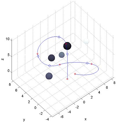
5.3. Obstacle Collision Detection

The path from Section 5.2 was used to test the obstacle detection algorithm on a standard 3.4-GHz desktop computer. Five spheres were placed in the vicinity of the curve, and the points on the path closest to each obstacle were calculated using two methods.
The first method discretized the trajectory into 1000 nodes and took 463 ms to find the closest position on the trajectory for each of the five obstacles. The second hybrid method uses a coarse discretization and then a numerical minimizer (as described in Section 4) to find the collision distance. The solution time for the hybrid method was 309 ms and is shown in Figure 5. The circles on the path mark the points where an obstacle was closest. The percentage difference between the two methods is 40%, so reduced computing time is possible, especially in cases were there are many obstacles. Additionally, since MATLAB is an interpreted language, it is slower than compiled code. If the algorithms were rewritten in a different language, such as C, and compiled, then the computation time would be reduced. However, since we are interested in comparing the methods, MATLAB was chosen for its ease of use.
Figure 5. Obstacle detection.
Aerospace 02 00155 g005

6. Conclusions

This paper presents a method for concatenating separate trajectories to form smooth, analytically-defined paths for a quadrotor along a set of waypoints. Since the functions are defined using analytical expressions, only a numerical minimizer is needed to calculate the optimisation vector that controls the shape of the curve. A controller was used to ensure that the generated trajectory is trackable and dynamically feasible. Additionally, it provided information about the thrust and moments required to fly a typical quadrotor along the trajectory. An obstacle detection algorithm is presented that is a hybrid method of discretizing the path into nodes and using a numerical minimizer to find the minimum collision distance to an obstacle. Compared to just discretizing the path, this method is faster and able to, more precisely, locate the correct collision distance.
Further work will look at using the analytically-defined curves for sample-based planning methods, allowing for a full path planning method that does not rely on the input of waypoints to navigate an area. This paper focuses on trajectory planning for quadrotor unmanned aerial systems, but the techniques used could also be applied to other types of vehicles.

Author Contributions

The paper was was written by Jonathan Jamieson and James Biggs assisted with the proof for the sub-Riemannian curves given in the Appendix.

Conflicts of Interest

The authors declare no conflicts of interest.

Appendix: Analytical Curves Proof

An application of the coordinate-free maximum principle [19,23] that minimizes Equation (10) subject to Equation (9) yields the Hamiltonian:
H ( p , u , g ) = v 3 p 3 + M 1 Ω 1 + M 2 Ω 2 ρ 0 2 ( v 3 2 + c ( Ω 1 2 + Ω 2 2 ) )
where ρ 0 = 1 for regular extremals and ρ 0 = 0 for abnormal extremals. In this paper, we only consider the regular extremals; therefore, we set ρ 0 = 1 . Noting that Equation (A1) is a concave function, then to satisfy the conditions of the maximum principle, we need H Ω i = 0 and H v i = 0 . The control functions are thus:
v 3 * = p 3 , Ω 1 * = M 1 c , Ω 2 * = M 2 c
Substituting Equation (A2) back into Equation (A1) gives the optimal Hamiltonian:
H * = 1 2 ( p 3 2 + M 1 2 c + M 2 2 c )
The corresponding Hamiltonian vector fields describing the necessary conditions for optimality are calculated using the Poisson bracket { p ^ ( · ) , p ^ ( · ) } = p ^ ( [ · , · ] ) where ( · ) s e ( 3 ) [19]. Then, the Hamiltonian vector fields are given by:
d ( · ) d t = { · , H * }
where ( · ) s e ( 3 ) * . Explicitly:
p ˙ 1 = M 2 p 3 c , p ˙ 2 = M 1 p 3 c , p ˙ 3 = p 1 M 2 M 1 p 2 c , M ˙ 1 = p 2 p 3 M 2 M 3 c , M ˙ 2 = p 1 p 3 + M 1 M 3 c , M ˙ 3 = 0
using the conserved quantity:
I 2 = p 1 2 + p 2 2 + p 3 2
and identifying a particular solution by assuming p ˙ 3 = 0 , we can reduce the conserved quantities to s 2 = M 1 2 + M 2 2 t , where s 2 = c ( 2 H * p 3 2 ) ; so we can write:
s 2 = M 1 ( 0 ) 2 + M 2 ( 0 ) 2
and defining r 2 = I 2 p 3 2 from Equation (A6), we can write r 2 = p 1 2 + p 2 2 t ; thus:
r 2 = p 1 ( 0 ) 2 + p 2 ( 0 ) 2
These reduced conserved quantities suggest using polar coordinates to solve the differential Equation (A5), so we try the ansatz solution:
M 1 = s cos ( α t + β ) , M 2 = s sin ( α t + β ) p 1 = r cos ( α t + β ) , p 2 = r sin ( α t + β )
where r and s are defined in Equations (A7) and (A8). Substituting into Equation (A5), we obtain the following two solutions for α:
α = s p 3 ( 0 ) c r , α = p 3 ( 0 ) r s M 3 ( 0 ) c
Thus, Equation (A9) is a particular solution if and only if:
M 3 ( 0 ) = p 3 ( 0 ) s 2 + c r 2 s r
Therefore, the particular solution in terms of the initial conditions are:
p 1 = r cos θ , p 2 = r sin θ , p 3 = p 3 ( 0 ) , M 1 = s cos θ , M 2 = s sin θ , M 3 = p 3 ( 0 ) s 2 + c r 2 s r
where θ = s p 3 ( 0 ) c r t + β and s and r are defined in terms of the initial conditions in Equations (A7) and (A8) and where β = atan 2 ( M 2 ( 0 ) , M 1 ( 0 ) ) . For convenience, define a constant K 2 = I 2 , where I 2 = r 2 + p 3 2 is the Casimir function Equation (A6), then as R S O ( 3 ) is known [19] to satisfy the equation:
R P R 1 = ρ
where P = p 1 E 1 + p 2 E 2 + p 3 E 3 and E 1 , E 2 and E 3 is a basis for the Lie algebra of S O ( 3 ) and ρ s o ( 3 ) is a constant matrix. This fact implies that any orbit R P R 1 = ρ is conjugate to ρ = K E 3 , and therefore, it suffices to integrate the particular orbit:
R p P R p 1 = K E 3
Then, let ϕ 1 , ϕ 2 and ϕ 3 denote the coordinates of a point in S O ( 3 ) according to the formula:
R p = exp ( ϕ 1 E 3 ) exp ( ϕ 2 E 2 ) exp ( ϕ 3 E 3 )
Then, substituting Equation (A15) into Equation (A14) yields:
P = K exp ( ϕ 3 E 3 ) exp ( ϕ 2 E 2 ) E 3 exp ( ϕ 2 E 2 ) exp ( ϕ 3 E 3 )
which gives:
P = K 0 cos ϕ 2 sin ϕ 2 sin ϕ 3 cos ϕ 2 0 sin ϕ 2 cos ϕ 3 sin ϕ 2 sin ϕ 3 sin ϕ 2 cos ϕ 3 0
recalling that p 3 = v 3 ( 0 ) , then:
r cos θ = K cos ϕ 3 sin ϕ 2 r sin θ = K sin ϕ 3 sin ϕ 2 p 3 ( 0 ) = K cos ϕ 2
cos ϕ 2 = p 3 ( 0 ) r 2 + p 3 ( 0 ) 2 , sin ϕ 2 = r r 2 + p 3 ( 0 ) 2
and as tan θ = tan ϕ 3 , then ϕ 3 = θ . To calculate ϕ 1 , substitute (A15) into (4), and we can obtain the following relationships:
sin ϕ 2 sin ϕ 3 ϕ ˙ 1 + cos ϕ 3 ϕ ˙ 2 = Ω 2 * sin ϕ 2 cos ϕ 3 ϕ ˙ 1 + sin ϕ 3 ϕ ˙ 2 = Ω 1 *
which can be manipulated to give:
ϕ ˙ 1 = Ω 2 * sin ϕ 3 Ω 1 * cos ϕ 3 sin ϕ 2
which can be simplified and integrated assuming ϕ 1 ( 0 ) = 0 to yield:
ϕ 1 = ( s r 2 + p 3 ( 0 ) 2 r c ) t
substituting all of the values into Equation (A15) to obtain a particular optimal solution for R p , we can then obtain x p analytically by integration of the equation d x p d t = R p v to give Equation (11). These analytic solutions for x p and R p can then be used to form a particular solution g p ( t ) of Equation (8). For convenience, we pull this solution back to the identity by computing g ( t ) = g p ( 0 ) 1 g p ( t ) , so that the quadrotor starts at the origin; then, x p Equation (11) is obtained via the following projection [ 1 x ] T = g . [ 1 0 0 0 ] T . The following notation has been used in Equation (11, 12,13,14,15,16,17): λ 1 = M 1 ( 0 ) , λ 2 = M 2 ( 0 ) , λ 3 = p 1 ( 0 ) , λ 4 = p 2 ( 0 ) and ν = v 3 .

References

  1. Matsumoto, T.; Kita, K.; Suzuki, R.; Oosedo, A.; Go, K.; Hoshino, Y.; Konno, A.; Uchiyama, M. A hovering control strategy for a Tail-Sitter VTOL UAV that increases stability against large Disturbance. In Proceedings of the 2010 IEEE International Conference on Robotics and Automation (ICRA 2010), Anchorage, AK, USA, 3–8 May 2010; pp. 54–59.
  2. Mueller, M.W.; Hehn, M.; D’Andrea, R. A computationally efficient algorithm for state-to-state quadrocopter trajectory generation and feasibility verification. In Proceedings of the 2013 IEEE/RSJ International Conference on Intelligent Robots and Systems (IROS 2013), Tokyo, Japan, 3–7 November 2013; pp. 3480–3486.
  3. Bouktir, Y.; Haddad, M.; Chettibi, T. Trajectory planning for a quadrotor helicopter. In Proceedings of the 2008 16th Mediterranean Conference on Control and Automation, Ajaccio Corsica, France, 25–27 June 2008; pp. 1258–1263.
  4. Babel, L. Three-dimensional route planning for unmanned aerial vehicles in a risk environment. J. Intell. Robot. Syst. 2013, 71, 255–269. [Google Scholar] [CrossRef]
  5. Lizarraga, M.; Elkaim, G. Spatially deconflicted path generation for multiple UAVs in a bounded airspace. In Proceedings of the 2008 IEEE/ION Position, Location and Navigation Symposium, Monterey, CA, USA, 5–8 May 2008; pp. 1213–1218.
  6. Lewis, L.R.; Ross, I.M.; Gong, Q. Pseudospectral motion planning techniques for autonomous obstacle avoidance. In Proceedings of the 2007 46th IEEE Conference on Decision and Control, New Orleans, LA, USA, 12–14 December 2007; pp. 5997–6002.
  7. Lewis, L.P.R. Rapid Motion Planning and Autonomous Obstacle Avoidance for Unmanned Vehicles. Ph.D. Thesis, Naval Postgraduate School, Monterey, CA, USA, 2006. [Google Scholar]
  8. Lin, Y.; Saripalli, S. Path planning using 3D dubins curve for unmanned aerial vehicles. In Proceedings of the 2014 IEEE International Conference on Unmanned Aircraft Systems (ICUAS 2014), Orlando, FL, USA, 27–30 May 2014; pp. 296–304.
  9. Van den Berg, J.; Lin, M.; Manocha, D. Reciprocal velocity obstacles for real-time multi-agent navigation. In Proceedings of the IEEE International Conference on Robotics and Automation (ICRA 2008), Pasadena, CA, USA, 19–23 May 2008; pp. 1928–1935.
  10. Shim, D.H.; Sastry, S. An evasive maneuvering algorithm for UAVs in see-and-avoid situations. In Proceedings of the 2007 IEEE American Control Conference (ACC 2007), New York, NY, USA, 9–13 July 2007; pp. 3886–3891.
  11. Jamieson, J.; Biggs, J. Trajectory generation using sub-riemannian curves for quadrotor UAVs. In Proceedings of the 2015 European Control Conference (ECC 2015), Linz, Austria, 15–17 July 2015.
  12. Bouabdallah, S. Design and Control of Quadrotors with Application to Autonomous Flying. Ph.D. Thesis, Swiss Federal Institute of Technology in Lausanne, Lausanne, Switzerland, 2007. [Google Scholar]
  13. Martinez, V. Modelling of the Flight Dynamics of a Quadrotor Helicopter. M.Sc. Thesis, Cranfield University, Bedford, UK, 2007. [Google Scholar]
  14. Amir, M.; Abbass, V. Modeling of quadrotor helicopter dynamics. In Proceedings of the 2008 International Conference on Smart Manufacturing Application (ICSMA 2008), Goyang-si, Korea, 9–11 April 2008; pp. 100–105.
  15. Lee, T.; Leoky, M.; McClamroch, N. Geometric tRacking control of a quadrotor UAV on SE(3). In Proceedings of the 2010 49th IEEE Conference on Decision and Control (CDC 2010), Atlanta, GA, USA, 15–17 December 2010; pp. 5420–5425.
  16. Biggs, J.; Holderbaum, W.; Jurdjevic, V. Singularities of optimal control problems on some 6-D Lie groups. IEEE Trans. Autom. Control 2007, 52, 1027–1038. [Google Scholar] [CrossRef] [Green Version]
  17. Biggs, J.; Holderbaum, W. Optimal kinematic control of an autonomous underwater vehicle. IEEE Trans. Autom. Control 2009, 54, 1623–1626. [Google Scholar] [CrossRef]
  18. Walsh, G.; Montgomery, R.; Sastry, S. Optimal path planning on matrix Lie groups. In Proceedings of the 33rd IEEE Conference Decision and Control, Lake Buena Vista, FL, USA, 14–16 December 1994; Volume 2, pp. 1258–1263.
  19. Jurdjevic, V. Geometric Control Theory; Cambridge University Press: Cambridge, UK, 1996. [Google Scholar]
  20. Deb, K.; Pratap, A.; Agarwal, S.; Meyarivan, T. A fast and elitist multiobjective genetic algorithm: NSGA-II. IEEE Trans. Evol. Comput. 2002, 6, 182–197. [Google Scholar] [CrossRef]
  21. Pounds, P.; Mahony, R.; Corke, P. Modelling and control of a large quadrotor robot. Control Eng. Pract. 2010, 18, 691–699. [Google Scholar] [CrossRef] [Green Version]
  22. Pounds, P.; Mahony, R.; Gresham, J.; Corke, P.; Roberts, J.M. Towards dynamically-favourable quad-rotor aerial robots. In Proceedings of the 2004 Australasian Conference on Robotics & Automation, Canberra, Australia, 26 April–1 May 2004.
  23. Sussmann, H.J. An introduction to the coordinate-free maximum principle. In Geometry of Feedback and Optimal Control; Jakubczyk, B., Respondek, W., Eds.; Marcel Dekker, Inc.: New York, NY, USA, 1997; pp. 463–557. [Google Scholar]

