Article

Variational Method-Based Trajectory Optimization for Hybrid Airships

1
Beijing Institute of Spacecraft Environment Engineering, Beijing 100094, China
2
Aerospace Times Feihong Technology Co., Ltd., Beijing 100094, China
3
China Aerospace Science and Technology Corporation, Beijing 100048, China
*
Author to whom correspondence should be addressed.
These authors contributed equally to this work.
Aerospace 2024, 11(4), 250; https://doi.org/10.3390/aerospace11040250
Submission received: 16 February 2024 / Revised: 14 March 2024 / Accepted: 21 March 2024 / Published: 22 March 2024

Abstract

:
Hybrid airships, combining aerodynamic lift and buoyant lift, are efficient near-space aircraft for scientific exploration, observation, and surveillance. Compared to conventional airplanes and airships, hybrid airships offer unique advantages, including stationary hovering and rapid deployment. Due to the different task requirements and strong coupling between flight and environment, trajectory-optimization methods for traditional aircraft are difficult to apply to hybrid airships directly. We propose a trajectory-optimization model based on the variational method to calculate the optimal time and energy paths under weak, uniform, and latitudinal linear wind fields. Our model shows that the influencing factors for the optimization path can be categorized into three types: airship design parameters, wind field parameters, and departure parameters. The result indicates that the optimal time paths are generally straight lines, and the optimal energy paths are piecewise curves with a 24-h cycle under typical hybrid airship design parameters. This work has provided new insight into the trajectory optimization and parameter design of future hybrid airships.

1. Introduction

With the increasing value of near-space platforms in communications, observation, surveillance, and scientific exploration, high payload and long endurance missions have become growing requirements for modern aircraft [1,2,3]. Hybrid airships, combining aerodynamic lift and buoyant lift [4], have advantages such as larger cargo capacities than aircraft and faster speeds than ships and rail [5]. The first experimental hybrid airship prototype can be traced back to AEREON III [6], which was manufactured by the AEREON corporation in 1960 but was destroyed during a taxiing test. In 1970, Boeing-Vertol Company and Goodyear Aerospace Corporation conducted a feasibility study on modern airships for NASA, which further precipitated the development of hybrid airship concepts [7]. The successful demonstration of the technology demonstrator SkyKitten by the Advanced Technologies Group in 2000 [8] marked a significant shift from conceptualization to practical implementation in hybrid airship research. However, feasibility study of the new hybrid airship continues to be the primary focus of research, such as the parameter calculations and performance analysis of the disk-shaped vehicle performed by Pisarevskiy et al. [9].
In recent years, this has become one of the broadest research areas in the field of aeronautical transportation, spurred by the rapid development of composite materials, flexible solar cells, and so on. Many companies are committed to the technology of hybrid airships, including Aero Vehicles Inc., China Aviation Industry General Aircraft Corp., Ltd. and Worldwide Aeros Corp., Boeing, and Lockheed Martin.
Several research aspects [10,11,12,13,14] of hybrid airships, consisting of conceptual design, stability analysis, and trajectory optimization, must consider the strong coupling with environmental factors due to its power source and unique lift source. Regarding conceptual design [15], the most widely studied aspect of hybrid airships, multi-disciplinary models [16,17,18], have often been adopted to consider the coupling between the environment and airships. On the basis of multi-disciplinary models, Meng et al. [19] propose a Concurrent Subsystem Optimization algorithm based on Response Surface (CSSO-RS) to calculate and optimize total mass of a hybrid airship. Manikandan and Pant [20] describe a multi-disciplinary design methodology for a tri-lobed envelope high-altitude airship from four disciplines, containing envelope geometry, aerodynamics, operating environment, and solar irradiance.
The model for trajectory optimization of hybrid airships differs significantly from that of traditional aircraft due to the strong coupling between flight of hybrid airships and environmental factors, including wind fields and solar radiation. Furthermore, the purpose of hybrid airship trajectory optimization is also unique because of mission requirements for heavy payloads and long endurance. Traditional airplane path planning generally focuses on optimizing long-distance flight duration with path constraints and typically only considers the wind environment. Sridhar et al. [21] calculate the cruising aircraft wind-optimal trajectory, avoiding regions of airspace that facilitate persistent contrail formation by solving a nonlinear optimal control problem. While the trajectory optimization of traditional airships generally aims to achieve energy circulation during the cruising state by considering gradient wind fields and diurnal energy variations in a small-scale range, Zhu et al. [22] studied the optimal closed trajectory for a stratospheric airship’s cruising in near-space via a collocation approach in three typical wind fields. Based on the aforementioned reasons, there is currently limited research on trajectory optimization for hybrid airships.
Hybrid airships combine the flight characteristics of both airplanes and airships, which are also evident in trajectory optimization, and require considering wind and solar radiation environments over a wide range of conditions. The key difference between hybrid airships and traditional platforms is the significantly constraining effect of environmental factors on the flight process. In contrast, the flight paths of traditional aircraft and airships are usually only determined by missions. Therefore, planning long-distance flight trajectories to optimize performance in terms of deployment time and payload working time is the new question driven by mission requirements and the characteristics of hybrid airships.
This paper develops a trajectory-optimization approach based on the variational method through the conversion of flight deployment and payload working time into the parameters of flight consumption time t and remaining flight energy E, with the aim of providing new insights for trajectory optimization of hybrid airships.
Section 2 provides the functional path model of time and energy based on the balance between lift and gravitational weight. Section 3 explains the optimal time and energy trajectory generation for hybrid airships. Conclusions and discussion are presented in Section 4.

2. Time and Energy Path Functionals for Hybrid Airship

For a set of path curves F ( x , y , z ) = 0 G ( x , y , z ) = 0 with fixed starting and ending points, each curve corresponds to a unique time t and energy E within the accurate number range. Thus, time t and energy E can be seen as functionals of the path curves y ( x ) , expressed as t = t [ y ( x ) ] and E = E [ y ( x ) ] . When disregarding small variations in the altitude of the airship during cruise, the state of a hybrid airship can be represented as:
G = F b + F l
in which G is the total weight of the airship, F b is the buoyancy lift and F l is the aerodynamic lift. Equation (1) can be written as:
m g = ρ g V + 1 2 ρ C L v 2 b
where m is the total mass of the airship; ρ is the density of air; V is the volume of the airship’s buoyant body; C L is the aerodynamic lift coefficient; v is the airspeed of the airship; b is the aerodynamic chord length of the hybrid airship.
According to the velocity relationship, as shown in Figure 1, the expression for airspeed leads to:
v = v v w cos ( φ + θ + π 2 )
in which v and φ are the magnitude and direction of the absolute velocity of the airship with respect to the ground; v w and θ are the magnitude and direction of wind speed.
Combining the definition of magnitude and direction of absolute velocity, v = d s d t and sin φ = d y d s , Equation (3) yields:
d s d t = v v w ( sin θ d x d s + cos θ d y d s )
where d s is the path differential defined as d s = d x 2 + d y 2 . Now the time differential d t can be written as:
d t = d x 2 + d y 2 v v w ( sin θ d x + cos θ d y d x 2 + d y 2 )
For path time, applying time differential (5) yields:
t [ y ( x ) ] = t 1 t 0 = l d t = l 1 + y 2 v 1 + y 2 v w ( sin θ + y cos θ ) d x = x 0 x 1 1 + y 2 v 1 + y 2 v w ( sin θ + y cos θ ) d x
where t 1 and t 0 are the end and start times of the airship flight; l is the flight path; y is the path derivative defined as y = d y d x .
Further, we obtain the math representation for the flight time minimization problem:
x 0 x 1 1 + y 2 v 1 + y 2 v w ( sin θ + y cos θ ) d x = ! m i n y ( x 0 ) = y 0 , y ( x 1 ) = y 1
For path energy, also applying time differential (5) yields:
E [ y ( x ) ] = E i n E o u t = l P i n d t ( l F D d s + l C d t ) = x 0 x 1 ( P i n C ) ( 1 + y 2 ) v 1 + y 2 v w ( sin θ + y cos θ ) 1 2 ρ C D v 2 b 1 + y 2 d x = x 0 x 1 ( P i n C ) ( 1 + y 2 ) v 1 + y 2 v w ( sin θ + y cos θ ) ( m g ρ g V ) C D C L 1 + y 2 d x
in which E i n and E o u t are the input and output energy of an airship flight. The input energy is derived from the solar energy absorption by solar panels, and the output energy consists of the energy dissipated by aerodynamic drag and consumed by the airship control system. P i n is the absorbed power of solar panels; F D is the aerodynamic drag of airship; C is the power of airship control system.
We also obtain the math representation for the flight energy minimization problem:
x 0 x 1 ( P i n C ) ( 1 + y 2 ) v 1 + y 2 v w ( sin θ + y cos θ ) ( m g ρ g V ) C D C L 1 + y 2 d x = ! m i n y ( x 0 ) = y 0 , y ( x 1 ) = y 1
Therefore, the above minimization problem can be solved using the variational method and the Euler equation as follows:
d d x L y L y = 0
in which the Lagrangian function L is required to be a second-order differential function of x, y, and y .
The Lagrangian functions of time and energy can be written as:
L t ( x , y , y ) = 1 + y 2 v 1 + y 2 v w ( sin θ + y cos θ ) L E ( x , y , y ) = ( P i n C ) ( 1 + y 2 ) v 1 + y 2 v w ( sin θ + y cos θ ) ( m g ρ g V ) C D C L 1 + y 2
where P i n is a nonsmooth function written as:
P i n = I S max ( sin h , 0 ) = I S max ( sin φ sin δ + cos φ cos δ cos ω , 0 ) = I S sin φ sin δ + cos φ cos δ cos ω + | sin φ sin δ + cos φ cos δ cos ω | 2
in which I is the solar radiation power, S is the effective area of the solar panel; h is the solar altitude angle; φ is the geographic latitude; δ is the solar declination angle; ω is the solar hour angle. In this paper, design parameters of a typical hybrid airship are shown in Table 1.
Therefore, we transform the function P i n into a Fourier series to satisfy the second-order differentiability of the energy Lagrangian function for x, y, and y .
For function y = | sin x | , the Fourier series can be expressed as:
y = 2 π 4 π ( cos 2 x 1 · 3 + cos 4 x 3 · 5 + cos 6 x 5 · 7 + )
Further, we obtain the Fourier series of P i n :
P i n = I S [ 1 π + 1 2 sin h 2 π ( cos 2 x 1 · 3 + cos 4 x 3 · 5 + cos 6 x 5 · 7 + ) ]
The Fourier series of function P i n up to the 4th order is shown in Figure 2. In this paper, we take the 3rd-order Fourier series for subsequent calculations.
Applying the trigonometric double-angle formula to avoid introducing arcsin h , the function of P i n is obtained:
P i n = I S ( 1 7 π + 1 2 sin h + 24 7 π sin 2 h 80 21 π sin 4 h + 64 35 π sin 6 h ) sin h = sin δ sin φ + cos δ cos φ cos ω φ = 180 π · y R δ = 23.45 · sin ( 360 · 284 + n 0 365 ) ω = 15 · ( t + t 0 ) 180
in which n 0 is the number of days inclusive from 1 January to the airship departure date ( δ = 0 on the vernal equinox); t and t 0 are the flight time and departure time.

3. Time and Energy Optimal Path Analysis for a Hybrid Airship under a Known Wind Field

The optimal paths of time and energy vary under different wind field environments due to the influence of wind field variables ( v w and θ ) on the representation of the Lagrangian function L t and L E . Therefore, time and energy optimal paths are quantitatively analyzed under the following three wind fields based on the U.S. Naval Research Laboratory Horizontal Wind Model [23,24] shown in Figure 3.

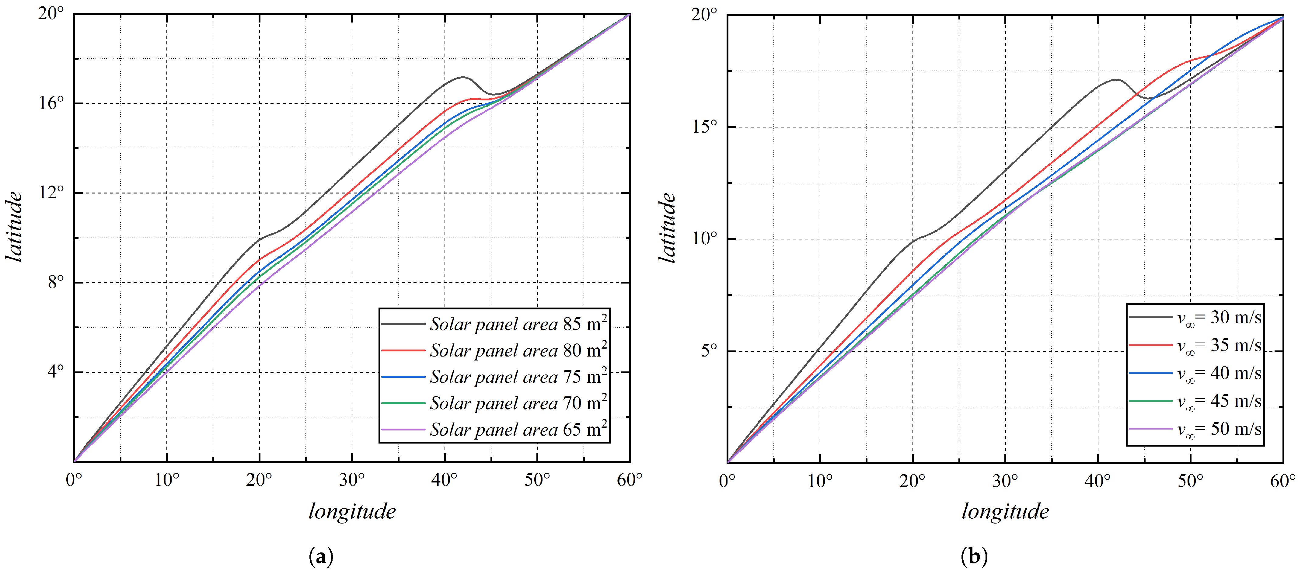
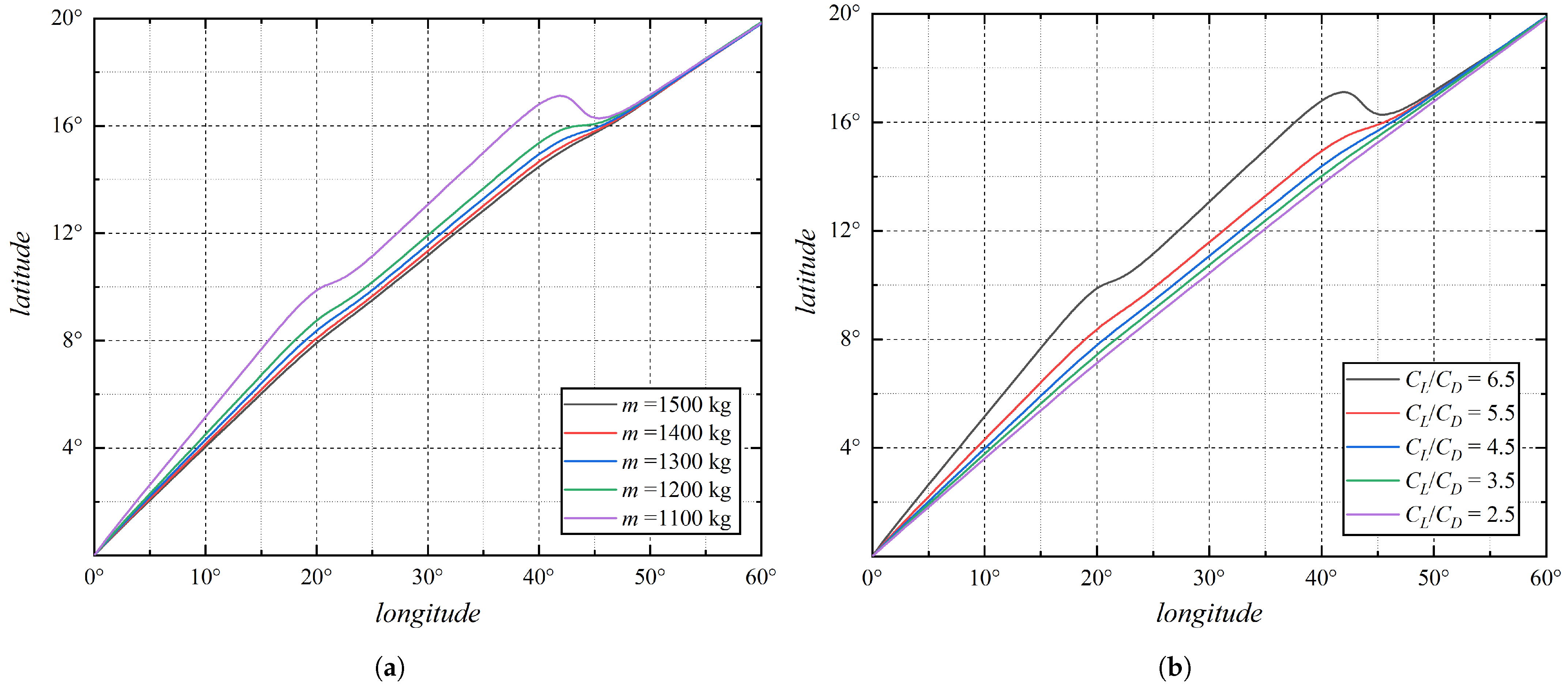
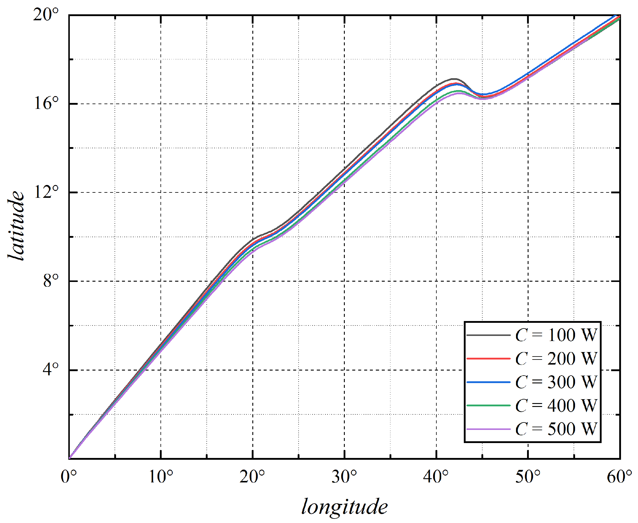
3.1. Weak Wind Field

We refer to the environment where the magnitude of wind speed v w is significantly smaller than the air speed v as a weak wind field. Regarding the Lagrangian function L t and L E , v 1 + y 2 v w ( sin θ + y cos θ ) , Equation (11) yields:
L t ( x , y , y ) = 1 + y 2 v L E ( x , y , y ) = [ P i n C v ( m g ρ g V ) C D C L ] 1 + y 2
For the Lagrangian function of path time L t 1 , the Euler equation is reduced to:
L t 1 y = C 1
Based on Equation (17), the time-optimal path is the line passing through the starting and ending points, shown as Equation (18), which means that the time-optimal flying trajectory for every hybrid airship under a weak wind field is straight-line flight.
y = y 1 y 0 x 1 x 0 ( x x 0 ) + x 0
When the Lagrangian function of path energy L E 1 is denoted as L E 1 ( x , y , y ) = P ( x , y ) 1 + y 2 , the Euler equation is reduced to:
y 1 + y 2 P ( x , y ) + y P x P y = 0
The mapping between path time and coordinates is established through the time consumption of the straight flight:
t x 2 + y 2 v
Together with Equations (15), (19) and (20), the Euler equation becomes:
( 1 2 + 48 7 π sin h 320 21 π sin 3 h + 384 35 π sin 5 h ) · [ π 12 cos δ cos φ sin ω ( y x y v x 2 + y 2 ) sin δ cos φ cos δ sin φ cos ω R ] + y 1 + y 2 [ 1 7 π + 1 2 sin h + 24 7 π sin 2 h 80 21 π sin 4 h + 64 35 π sin 6 h C I S v ( m g ρ g V ) I S · C D C L ] = 0
Equation (21) represents a second-order implicit differential equation as a function of variables x and y, which poses challenges in obtaining an analytical solution. Therefore, this paper adopts the Lagrange form of the polynomial interpolation [25] for solving the differential equation, and the iterative formula for this approach is as follows:
F ( t n + 1 , y n + 1 , y n + 1 y n h ) = 0 F ( t n + 1 , y n + 1 [ m ] , y n + 1 [ m ] y n [ m ] h ) + ( 1 h F y + F y ) δ = 0
The model of a hybrid airship optimal energy path under a weak wind field has been established by Equation (21), which shows that the optimal path is under the influence of geographic latitude φ , solar declination angle δ , solar hour angle ω , total mass m, effective area of solar panel S, lift–drag ratio C L / C D , volume of the airship’s buoyant body V, air speed of the airship v .
Based on Equation (15), the airship departure date and time, n 0 and t 0 , respectively, affect the solar altitude angle by changing the solar declination angle and the solar hour angle. The optimal energy path, starting at 0 E and 0 N and ending at 60 E and 20 N (a typical weak wind field region chosen arbitrarily), under different departure months and times, is calculated and shown in Figure 4.
The results indicate that optimal energy paths are piecewise with around three 24 h cycles under our conditions. In the calculated range, due to direct sunlight in the northern hemisphere during summer, the higher the latitude, the greater the maximum solar altitude angle and radiation power received. Therefore, the paths of May, July, and September tend to be concentrated at higher latitudes, and this trend becomes more pronounced as the summer solstice approaches. Conversely, the paths of January, March, and November tend to be situated at lower latitudes, as shown in Figure 4a. Additionally, it should be noted that the departure time on the same day only affects the phase of the solar hour angle. Consequently, energy paths with the same departure date but different instants of the day exhibit a translational similarity, as illustrated in Figure 4b.
Unlike parameters that are associated with the departure, design-related parameters such as total mass m, effective area of solar panel S, lift–drag ratio C L / C D , volume of the airship’s buoyant body V, air speed of the airship v do not exert influence on the differential equations by altering the solar altitude angle. Instead, they modify the two negative terms about airship design parameters within the differential equations. The design parameters without minus are as follows:
C I S + v ( m g ρ g V ) I S · C D C L
Similarly, starting from the initial position at 0 degrees, we aim to determine the optimal energy path for different design parameter values, with the final destination at a latitude of 20 N and a longitude of 60 E, as shown in Figure 5, Figure 6 and Figure 7.
The findings imply that, given identical departure parameters, augmenting the effective area of the solar panel, enhancing the lift–drag ratio, decreasing the airspeed, and diminishing the total design mass can cause a decline in the design parameters, which would culminate in an increase in the curvature of the optimal energy-path curve. The reason for this lies in the fact that the design parameters act as a representation of the portion of power dissipated through aerodynamic drag relative to the solar input power. When aerodynamic drag becomes a substantial component of the overall power consumption, the energy path of the hybrid airship tends to portray a reduced length, aiming to alleviate the exertion caused by drag. Considering that the power of airship control system C is generally significantly smaller in magnitude compared to the power dissipation resulting from air resistance, the influence of C on optimal energy-path design remains relatively insignificant unless there are substantial alterations in orders of magnitude. Under a weak wind field, the airspeed of hybrid airships, which is equal to the absolute velocity, affects the optimal energy paths by influencing the local solar altitude angle and design parameter terms. However, the optimal energy paths gradually tend towards straight lines as the airspeed increases, similar to the increase in total mass. The above calculations, which clarify the impact of two types of parameters on trajectory optimization, still have limitations because the weak wind field generally exists in low-latitude regions. Furthermore, wind field parameters are required for accurate calculations and analysis.

3.2. Uniform Wind Field

In this paper, uniform wind field refers to an aerodynamic setting where the magnitude and direction of the wind velocity exhibit no spatial variance during flight, v w , θ = c o n s t a n t . For Lagrangian function of path time L t 2 F ( y ) , the time optimal path coincides with Equation (18) with omission of details due to its evident calculation process.
Let the Lagrangian function of path energy L E 2 be denoted as L E 2 P ( x , y ) M ( y ) N ( y ) ; the Euler equation is reduced to:
d d x L E 2 y L E 2 y = P x · M y + P y · ( y M y M ) + ( P · 2 M y 2 2 N y 2 ) y
The mapping between path time and coordinates is established through the time consumption of a straight-line flight:
t x 2 + y 2 v x 2 + y 2 v w ( y cos θ + x sin θ )
Together with Equations (15), (24), and (25), the Euler equation becomes:
1 2 + 48 7 π sin h 320 21 π sin 3 h + 384 35 π sin 5 h · sin δ cos φ cos δ sin φ cos ω R 2 v w y cos θ + v w sin θ 1 y 2 v 1 + y 2 π cos δ cos φ sin ω 12 v x 2 + y 2 v w y cos θ + x sin θ 2 v 2 x y y 1 + y 2 x 2 + y 2 + 2 v w 2 y x 2 y 2 2 v w 2 x y 1 y 2 + v w v y 2 x 2 1 + y 2 cos θ + y sin θ + v w v 1 y 2 x 2 + y 2 x cos θ + y sin θ + 2 v w v y x 2 + y 2 y cos θ x sin θ + 2 v w v 1 + y 2 x y sin θ y cos θ y 1 7 π + sin h 2 + 24 7 π sin 2 h 80 21 π sin 4 h + 64 35 π sin 6 h C I S · v 2 + 2 v w 2 3 v w v sin θ + y cos θ 1 + y 2 v 1 + y 2 v w sin θ + y cos θ m g ρ g V I S C D C L v 1 + y 2 v w sin θ + y cos θ 2 1 + y 2 3 / 2 = 0
The introduction of both the magnitude and direction of wind speed increases the complexity of Equation (26). To clarify the results and discussions, we should maintain a constant airspeed v in the calculations for this section. The optimal energy path, also starting at 0 E, 0 N and ending at 60 E and 20 N, under different magnitudes and directions of wind velocity, are calculated and shown in Figure 8 to make a direct comparison with the results from the previous section.
With a similar conclusion to the preceding section, the optimal energy paths in uniform wind fields are also piecewise. When a hybrid airship maintains a constant buoyant lift in steady flight, the velocity relative to the air that sustains aerodynamic lift remains fixed. Therefore, with the absolute velocity of the airship decreasing due to increased wind speed, the airship experiences longer exposure to solar radiation, causing its tendency to soar at higher latitudes to increase total energy input, as shown in Figure 8a. The direction of an airship flight at the junction of piecewise optimal energy paths tends to be opposite to the direction of the wind. In this scenario, the airship, with its low absolute velocity, can achieve an extended flight duration at higher latitudes, which amplifies the total energy input, as shown in Figure 8b. The calculation of the impact of parameters of departure time and date and design parameters is analogous to the results mentioned in the previous section. Hence, they will not be further elaborated on here.
Due to the presence of uniform wind fields in high-latitude regions, the consideration of the airship departure latitude becomes indispensable when calculating the optimal energy path. With the increase in latitude, the path tends to a straight line because extreme values of solar altitude angle decrease, as shown in Figure 9.
Based on the above calculations and discussion, it is discernible that three categories are pivotal factors governing the optimal energy paths: airship design parameters, wind field parameters, and departure parameters. Specifically, the airship design parameters and wind field parameters establish the baseline for the optimal energy path. Furthermore, the departure parameters, including departure date, time, and latitude of the airship, exert influence on the energy path by modifying the local solar altitude angle. To be more general, we discussed the path under a latitudinal linear wind field, which is closer to natural conditions, in the subsequent section.

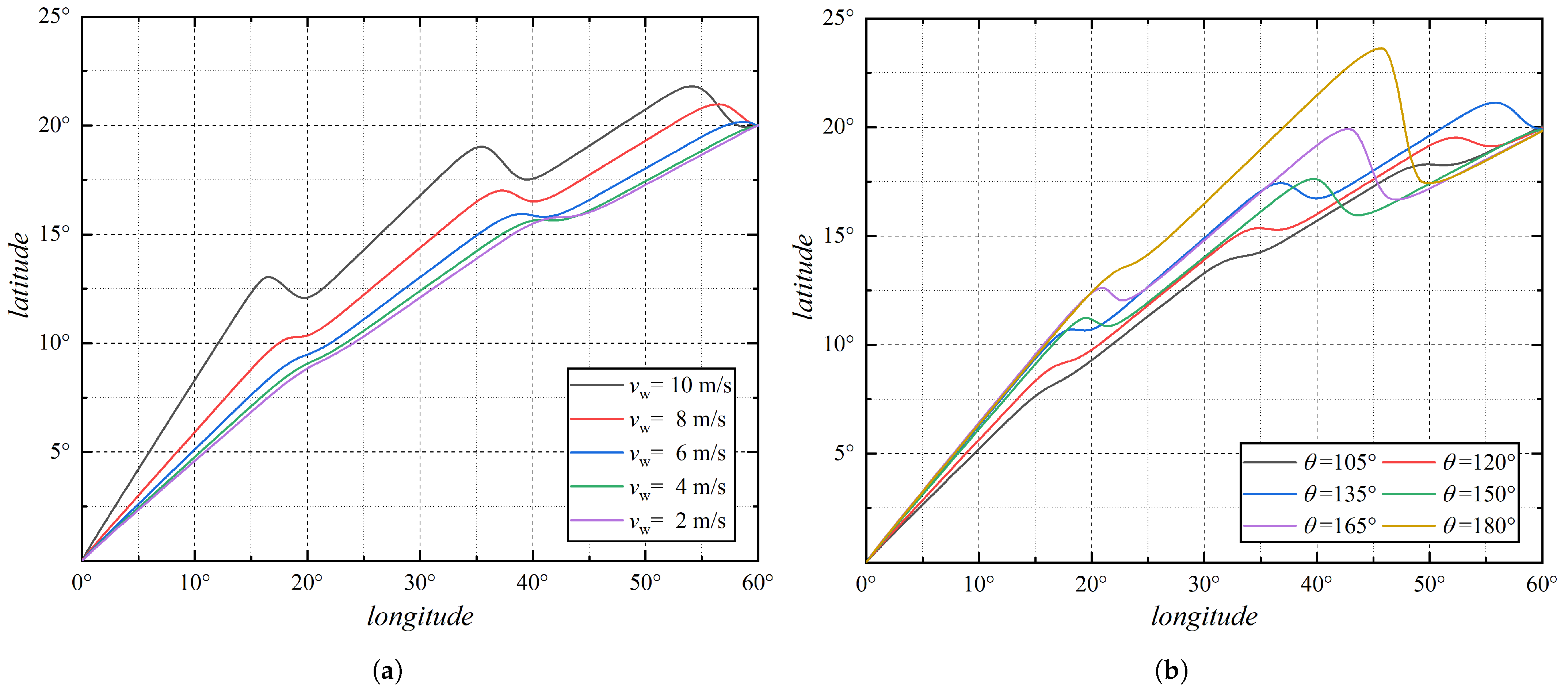
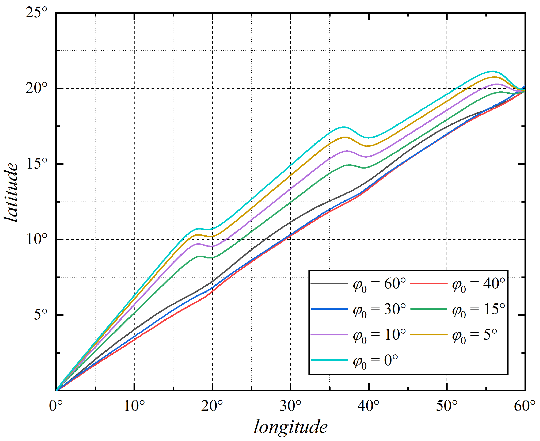
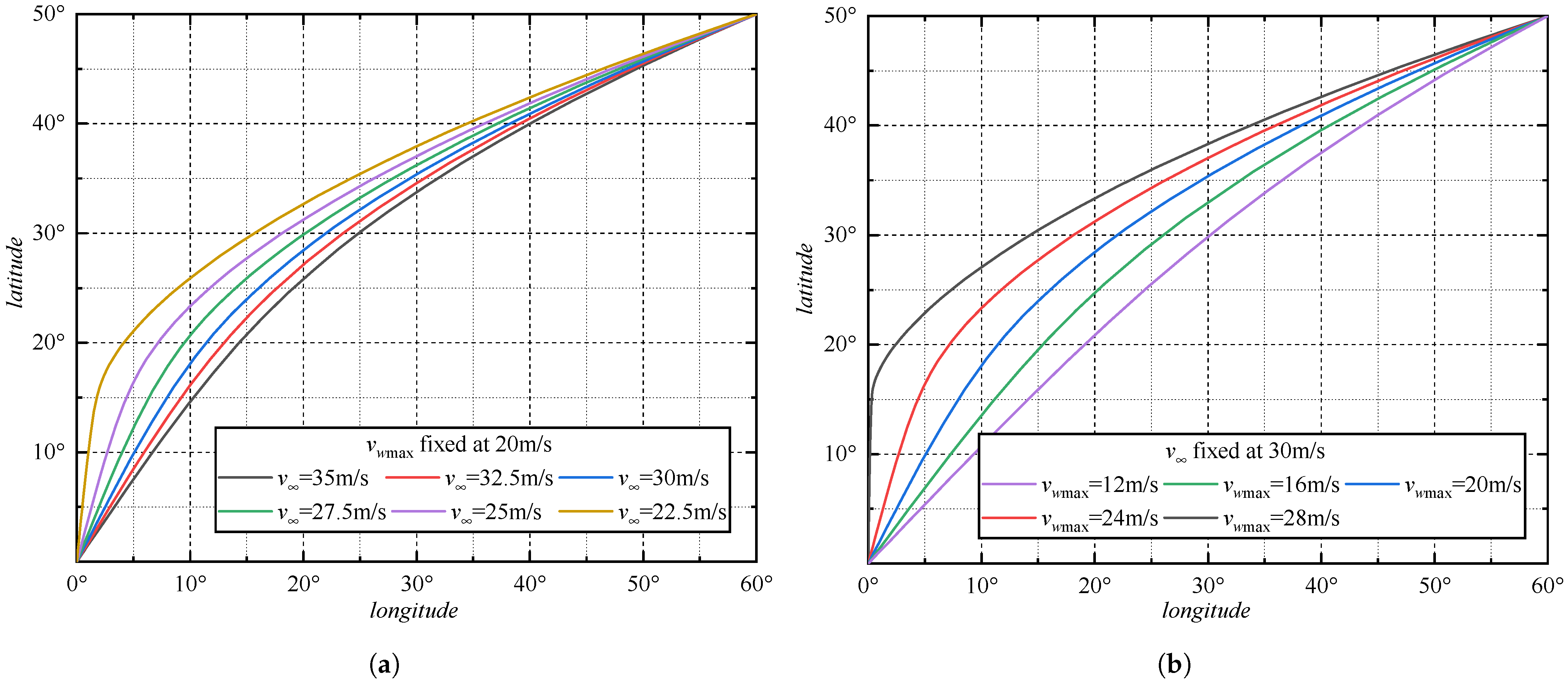
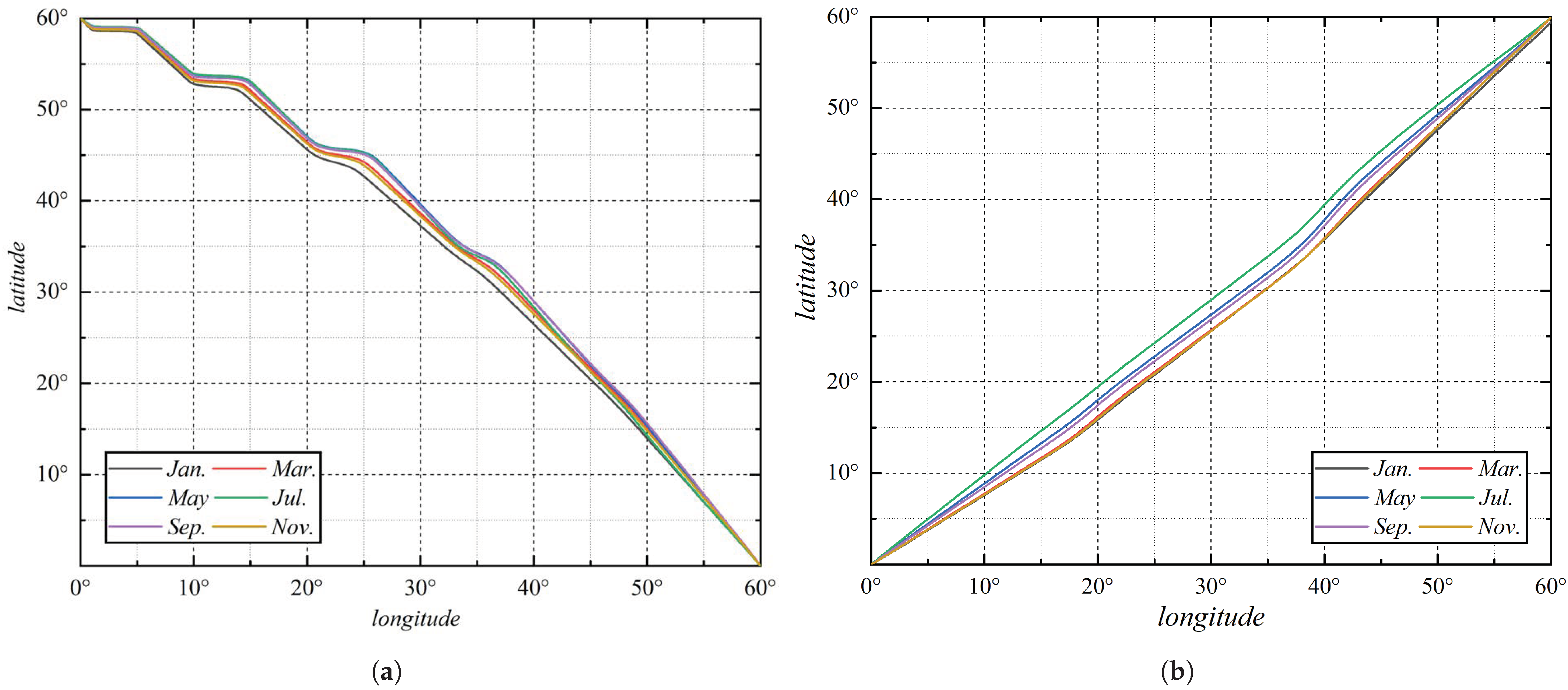
3.3. Latitudinal Linear Wind Field

The latitudinal linear wind field is defined as an atmospheric environment where the wind is directed perpendicular to the longitude lines, and its magnitudes vary linearly with latitude:
d v w d y = k , θ = 0
For the Lagrangian function of path time L t 3 :
L t 3 ( y , y ) = 1 + y 2 v 1 + y 2 k y y
Based on Equation (10), the Euler equation is reduced to:
v 1 + y 2 2 k y y ( v 1 + y 2 k y y ) 2 = C 1
The optimal time paths, starting at 0 E and 0 N and ending at 60 E and 50 N (the max wind speed at around 50 N based on Figure 3) are calculated under different relative velocities and wind speed gradients, as shown in Figure 10. Unlike previous results, the optimal time paths for latitudinal linear wind fields do not manifest as straight lines. However, the optimal time paths are close to straight lines, and this phenomenon is akin to the optimal energy paths in the uniform wind field under higher airspeed or more-minor wind gradient conditions.
Let the Lagrangian function of path energy L E 3 be denoted as L E 3 = f ( x , y ) · M ( y , y ) N ( y ) ; the Euler equation is reduced to:
d d x L E y L E y = d d x f · M y N y L E y = f 2 M y 2 2 N y 2 y + f 2 M y y + f y M y y + f x M y f y M f M y
The mapping between path time and coordinates is established through the time consumption of a straight-line flight:
t x 2 + y 2 k y 2 ln ( 1 k y 2 v x 2 + y 2 )
Together with Equations (15), (30), and (31), the Euler equation becomes:
y 1 7 π + sin h 2 + 24 7 π sin 2 h 80 21 π sin 4 h + 64 35 π sin 6 h C I S · v 1 + y 2 m g ρ g V I S 1 + y 2 3 / 2 C D C L + 1 7 π + sin h 2 + 24 7 π sin 2 h 80 21 π sin 4 h + 64 35 π sin 6 h C I S · 2 k y k y 2 + k y y v y y 1 + y 2 v 1 + y 2 k y y + 1 2 + 48 7 π sin h 320 21 π sin 3 h + 384 35 π sin 5 h · sin δ cos φ cos δ sin φ cos ω R 2 k y y v 1 + y 2 π cos δ cos φ sin ω 12 k x y y 2 1 + 2 k y y 2 + 2 x 2 x y + 2 x 2 + y 2 y v 1 + y 2 v x 2 + y 2 k y 2 + 2 x k y 2 ln 1 k y 2 v x 2 + y 2 · 2 k x y + k y y 2 k y y + x y v 1 + y 2 = 0
Based on Equation (32), the impact on the optimal energy paths under the four types of parameters mentioned in the previous section is not discussed again here. The optimal energy paths, starting from high latitudes to low latitudes (0 E, 60 N to 60 E, 0 N) and from low latitudes to high latitudes (0 E, 0 N to 60 E, 60 N), are calculated and shown in Figure 11 ( k = 0.013 s−1).
There is a significant difference in the optimal energy paths between the two sets of flight paths with different origins and destinations, but both follow the general trend of moving towards higher latitudes as the summer solstice approaches. When hybrid airships fly against the wind, their absolute velocity is lower during high-latitude flight than during low-latitude flight under a latitudinal linear wind field with higher winds at higher latitudes. Therefore, the optimal energy paths tend to be piecewise at high latitudes, similar to the previous section’s conclusion, as shown in Figure 11a. In contrast, the optimal energy paths tend to be straight lines to minimize power losses from drag dissipation due to the higher absolute velocity of hybrid airships flying with the wind, as illustrated in Figure 11b. The differences between the curves calculated under various departure months may not appear distinct in Figure 11 for the reason of variation in latitude scale. However, there is still a difference of 1 in the y-direction between the curves, equivalent to a maximum distance disparity of over 110 km. In conclusion, the optimal energy paths, influenced by the relative positions of the starting and ending points, need to be calculated based on specific mission requirements.

4. Discussion and Conclusions

In this study, we have applied functionals of the time and energy path curves for hybrid airships under three typical wind fields to calculate the optimal time and energy paths in weak, uniform, and latitude linear wind fields numerically using the Euler equation.
According to the calculated results, the optimal time paths are straight lines under weak or uniform wind field and curves when influenced by the air speed v and wind speed gradient k under the latitudinal linear wind field. However, the optimal energy paths are curves under typical wind fields in general. All influencing factors of optimal energy paths include the total mass m, effective area of solar panel S, lift–drag ratio C L / C D , volume of the airship’s buoyant body V, air speed of the airship v , magnitude v w and direction θ of wind speed, departure data n 0 , departure time t 0 , and departure latitude φ 0 , which can be categorized as airship design parameters, wind field parameters, and departure parameters.
The design parameters, including the effective area of solar panels, volume of the buoyancy body, lift–drag ratio, airspeed, and total mass, characterize the ratio of dissipated power to solar input power during flight. The optimal energy path tends to approach a straight line when the ratio is higher. However, a typical hybrid airship with a high lift–drag ratio, low airspeed, and large solar panel area cannot adopt a straight-line flight mode when maximizing its remaining energy. The wind field parameters, which consist of the magnitude and direction of the wind, affect the absolute speed of the hybrid airship. As the absolute velocity increases, the optimal energy paths tend to become straight lines. Additionally, the departure date, time, and latitude, referred to as departure parameters, impact the optimal energy paths by altering the local solar altitude angle.
We calculated that the time saved by the time-optimal path compared to straight-line flight, under the linear wind field with v w m a x = 25 m/s and v = 30 m/s (Section 3.3), is approximately 10.9 h, resulting in a direct improvement in transportation efficiency of 8.82%, and the efficiency value will increase as the wind gradient increases. This result implies that time-optimal path planning has the potential to enhance the cargo transportation capacity of hybrid airships.
While the significance of the optimal energy curve lies not only in improving the overall remaining energy but also in enhancing the energy cycling capability further. Based on our calculations, the optimal energy path for weak wind field on 1 July (Section 3.1) could increase the real-time power intake by approximately 246 W compared to straight-line flight, with an average power increase of about 111.7 W. Considering battery efficiency, the value is approximately 94.9 W. This value can be further improved conservatively to 150 W, considering the increased area and efficiency of solar panels, as well as the efficiency of the power-distribution system. This result means an additional enhancement in the payload capacity of the hybrid airship.
Furthermore, we can incorporate the analysis of optimal path design during the early stages of hybrid airship design based on the time and energy functional model presented before. This would enable us to estimate the hybrid airship’s arrival and hover time performance. There is still ample scope for refinement of the mapping relationship between path time and coordinates applied in this research, like introducing terms of velocity and acceleration to mapping in future studies. Furthermore, according to the time and energy functional, the arrival and hover time can be adopted as objective functions for hybrid airship parameter design, instead of just the total mass.
However, we recognize the limitations of this model as it is only applicable for path calculations in simplistic known wind fields. Our conclusions hold positive implications for trajectory optimization in less idealized environments during practical flights of hybrid airships.

Author Contributions

Conceptualization, W.G., Y.B. and X.Y.; methodology, W.G. and X.L.; software, W.G., A.D. and J.W.; formal analysis, W.G. and Y.B.; investigation, A.D. and J.W.; writing—original draft preparation, W.G., A.D. and Y.B.; writing—review and editing, W.G., Y.B., X.L., J.W. and X.Y.; Resources, W.G., A.D. and J.W.; Data Curation, W.G., W.G. and Y.B. contribute equally to the article. All authors have read and agreed to the published version of the manuscript.

Funding

This research was funded by Beijing Nova Program (Z211100002121077).

Data Availability Statement

No new data were created or analyzed in this study. Data sharing is not applicable to this article.

Conflicts of Interest

Author Apeng Dong is employed by the company Aerospace Times Feihong Technology Co., Ltd., Author Jing Wang is employed by the company China Aerospace Science and Technology Corporation. The remaining authors declare that the research was conducted in the absence of any commercial or financial relationships that could be construed as a potential conflict of interest.

References

  1. D’Oliveira, F.A.; de Melo, F.C.L.; Devezas, T.C. High-Altitude Platforms—Present Situation and Technology Trends. J. Aerosp. Technol. Manag. 2016, 8, 249–262. [Google Scholar] [CrossRef]
  2. Manikandan, M.; Pan, R.S. Research and advancements in hybrid airships—A review. Prog. Aerosp. Sci. 2021, 127, 100741. [Google Scholar]
  3. Yang, B.; Yang, J.; Li, X. The operating environment of near-space and its effects on the airship. Spacecraft Environ. Eng. 2008, 25, 555–557. [Google Scholar]
  4. Akshay, G.; Murugaiah, M.; Dushhyanth, R.; Dimitri, M. Conceptual Design and Feasibility Study of Winged Hybrid Airship. Aerospace 2022, 9, 8. [Google Scholar]
  5. Stockbridge, C.; Ceruti, A.; Marzocca, P. Airship Research and Development in the Areas of Design, Structures, Dynamics and Energy Systems. Int. J. Aeronaut. Space Sci. 2012, 13, 170–187. [Google Scholar] [CrossRef]
  6. Carichner, G.E.; Nicolai, L.M. Fundamentals of Aircraft and Airship Design; American Institute of Aeronautics and Astronautics: Reston, VA, USA, 2013; Volume 2—Airship Design and Case Studies, pp. 1–24. [Google Scholar]
  7. Ardema, M.D. Feasibility of Modern Airships: Preliminary Assessment. J. Aircr. 1977, 14, 1140–1148. [Google Scholar] [CrossRef]
  8. Mitchell, R. Effectiveness of Hybrid Airships as Cargo Airlifters. In Proceedings of the 11th AIAA Aviation Technology, Integration, and Operations (ATIO) Conference, Virginia Beach, VA, USA, 20–22 September 2011. [Google Scholar]
  9. Pisarevskiy, Y.V.; Fursov, V.B.; Pisarevskiy, A.Y.; Tatarnikov, P.N.; Sitnikov, N.V.; Goremykin, S.A. Electric hybrid airship with unlimited flight time. In Proceedings of the Sustainable Energy Systems: Innovative Perspectives (SES-2020), Saint-Petersburg, Russia, 29–30 October 2020. [Google Scholar]
  10. Carrin, M.; Biava, M.; Steijl, R.; Barakos, G.N.; Stewart, D. Computational fluid dynamics challenges for hybrid air vehicle applications. Adv. AeroSpace Sci. 2017, 9, 43–84. [Google Scholar]
  11. Carrion, M.; Biava, M.; Steijl, R.; Barakos, G.N.; Stewart, D. CFD Studies of Hybrid Air Vehicles. In Proceedings of the 54th AIAA Aerospace Sciences Meeting, San Diego, CA, USA, 4–8 January 2016. [Google Scholar]
  12. Pshikhopov, V.K.; Medvedev, M.Y.; Gaiduk, A.R.; Fedorenko, R.V.; Krukhmalev, V.A.; Gurenko, B.V. Position-Trajectory Control System for Unmanned Robotic Airship. In Proceedings of the 19th IFAC World Congress, Cape Town, South Africa, 24 August 2014. [Google Scholar]
  13. Prakash, O. Multibody Dynamics of winged Hybrid Airship Payload delivery System. In Proceedings of the AIAA Aviation 2020 Forum, Virtual, 15–19 June 2020. [Google Scholar]
  14. Anwar, U.H.; Waqar, A.; Erwin, S.; Jaffar, S.M.A.; Ali, O.A. Power-off static stability analysis of a clean configuration of a hybrid buoyant aircraft. In Proceedings of the 8th Ankara International Aerospace Conference 2015, Ankara, Turkey, 10–12 September 2015. [Google Scholar]
  15. Ceruti, A.; Marzocca, P. Conceptual Approach to Unconventional Airship Design and Synthesis. J. Aerosp. Eng. 2014, 27, 04014035. [Google Scholar] [CrossRef]
  16. Zhang, L.; Lv, M.; Meng, J.; Du, H. Conceptual design and analysis of hybrid airships with renewable energy. Proc. Inst. Mech. Eng. Part G J. Aerosp. Eng. 2018, 232, 2144–2159. [Google Scholar] [CrossRef]
  17. Zhang, L.; Lv, M.; Zhu, W.; Du, H.; Meng, J.; Li, J. Mission-based multidisciplinary optimization of solar-powered hybrid airship. Energy Convers. Manag. 2019, 185, 44–54. [Google Scholar] [CrossRef]
  18. Jiwei, T.; Weicheng, X.; Pingfang, Z.; Hui, Y.; Tongxin, Z.; Quanbao, W. Multidisciplinary Optimization and Analysis of Stratospheric Airships Powered by Solar Arrays. Aerospace 2023, 10, 43. [Google Scholar]
  19. Junhui, M.; Moning, L.; Nuo, M.; Li, L. Multidisciplinary design optimization of a lift-type hybrid airship. J. Beijing Univ. Aeronaut. Astronaut. 2021, 47, 72–83. [Google Scholar]
  20. Manikandan, M.; Pant, R.S. Conceptual Design Optimization of High-Altitude Airship Having a Tri-Lobed Envelope. In Advances in Multidisciplinary Analysis and Optimization; Springer: Singapore, 2022. [Google Scholar]
  21. Banavar, S.; Ng, H.K.; Chen, N.Y. Aircraft Trajectory Optimization and Contrails Avoidance in the Presence of Winds. J. Guid. Control. Dyn. 2011, 34, 1577–1584. [Google Scholar]
  22. Zhu, B.J.; Yang, X.-X.; Deng, X.-L.; Ma, Z.-Y.; Hou, Z.-X.; Jia, G.-W. Trajectory optimization and control of stratospheric airship in cruising. J. Numer. Math. 2019, 233, 1329–1339. [Google Scholar] [CrossRef]
  23. Hedin, A.E. Horizontal wind model (HWM) (1990). Planet. Space Sci. 1992, 40, 556–557. [Google Scholar] [CrossRef]
  24. Drob, D.P.; Emmert, J.T.; Meriwether, J.W.; Makela, J.J.; Doornbos, E.; Conde, M.; Hernandez, G.; Noto, J.; Zawdie, K.A.; McDonald, S.E.; et al. An update to the Horizontal Wind Model (HWM): The quiet time thermosphere. Earth Space Sci. 2014, 2, 301–319. [Google Scholar] [CrossRef]
  25. Shampine, L.F. Solving 0 = F(t, y(t), y’(t)) in Matlab. J. Numer. Math. 2002, 10, 291–310. [Google Scholar] [CrossRef]
Figure 1. The wind speed v w and the absolute velocity v of a hybrid airship at one point along a trajectory from start point A to end point B.
Aerospace 11 00250 g001
Figure 2. First- to fourth-order Fourier series of absorbed power of solar panels P i n .
Aerospace 11 00250 g002
Figure 3. Global wind field at altitude of 20 km on 1 January based on U.S. Naval Research Laboratory Horizontal Wind Model [23,24].
Aerospace 11 00250 g003
Figure 4. Optimal energy paths under different departure months at 12:00 ((a) left) and under different departure times on 1 July ((b) right).
Aerospace 11 00250 g004
Figure 5. Optimal energy paths under the different effective areas of solar panels ((a) left) and under different air speeds ((b) right).
Aerospace 11 00250 g005
Figure 6. Optimal energy paths under different total masses ((a) left) and under different lift–drag ratios ((b) right).
Aerospace 11 00250 g006
Figure 7. Optimal energy paths under different powers of airship control system.
Aerospace 11 00250 g007
Figure 8. Optimal energy paths under different magnitudes ((a) left) and directions ((b) right) of constant wind velocity.
Aerospace 11 00250 g008
Figure 9. Optimal energy paths under different departure latitudes.
Aerospace 11 00250 g009
Figure 10. Optimal time paths under different airspeeds ((a) left) and wind gradients ((b) right).
Aerospace 11 00250 g010
Figure 11. Optimal energy paths under different departure months from high latitudes to low latitudes ((a) left) and from low latitudes to high latitudes ((b) right).
Aerospace 11 00250 g011
Table 1. Typical design parameters of a hybrid airship for trajectory optimization.
Design ParameterValueUnit
v 30m/s
m1200kg
V9545m3
S85 × 0.12m2
I1367W/m2
C L / C D 6.5unitless
Disclaimer/Publisher’s Note: The statements, opinions and data contained in all publications are solely those of the individual author(s) and contributor(s) and not of MDPI and/or the editor(s). MDPI and/or the editor(s) disclaim responsibility for any injury to people or property resulting from any ideas, methods, instructions or products referred to in the content.

