To explain the definition of this static margin, consider the usual definition of a body reference frame, as proposed in
Figure 1. For simplicity, assume that the missile (or aircraft) is flying with a velocity vector aligned with
. Suppose now a perturbation is introduced in the direction of the velocity vector, such that a change in
, defined in
Figure 2, captures the overall intensity of the perturbation. Considering the front body plane of the aircraft, normal to
, it is possible to define a single plane so as to fully contain the perturbed velocity vector, while being normal to the front plane. This plane is here defined as the
plane. For example, in
Figure 7 the front body plane normal to
is shown with the corresponding cross-section of an example three-finned missile. The dashed line marks the plane normal to the front body plane and containing the velocity vector, i.e., the
plane.
Furthermore, the two plots on
Figure 7 show the decomposition of the aerodynamic force and moments ensuing from a velocity vector misaligned with respect to
, both with respect to the body reference axes (blue) and to a rotated reference (red). The latter, indicated as
, shares the first axis with the original body reference so that
, whereas axes
and
are defined in the
plane and normal to it, respectively. This can be equivalently described by defining the new
reference as rotated by an angle
around
with respect to the original body reference.
3.1. Assessing Static Stability via the Compounded Static Margin
While the newly introduced compounded static margin is capable of overcoming the limits of a static stability assessment based on the longitudinal and directional stability for an axial symmetric body (as will be shown in the next
Section 4), its ability to describe the level of static stability in a typical winged configuration is worse than that of the classical stability indexes currently employed.
In order to highlight the effectiveness and limits of the compounded index of static stability, an investigation is presented for four different body configurations. These configurations are chosen specifically to highlight that the more a body is able to respond to a perturbation in any direction, the more relevant the compounded margin becomes. This conceptual analysis was carried out with the help of numerical computations, employing the code
Tucan OpenVogel [
14], a software based on a vortex lattice method to estimate the aerodynamic coefficients of classic geometries consistent with all the hypotheses of potential flow theory.
The focus in the analysis is on understanding the existing correlation between the aerodynamic force and moment components associated with an assigned direction of the velocity vector. The conceptual test case scenarios consist of bi-dimensional half-wings with symmetric airfoils, characterized by the geometric parameters listed in
Table 3 and defined in
Figure 8. The so-defined lifting surface is arranged to produce different configurations.
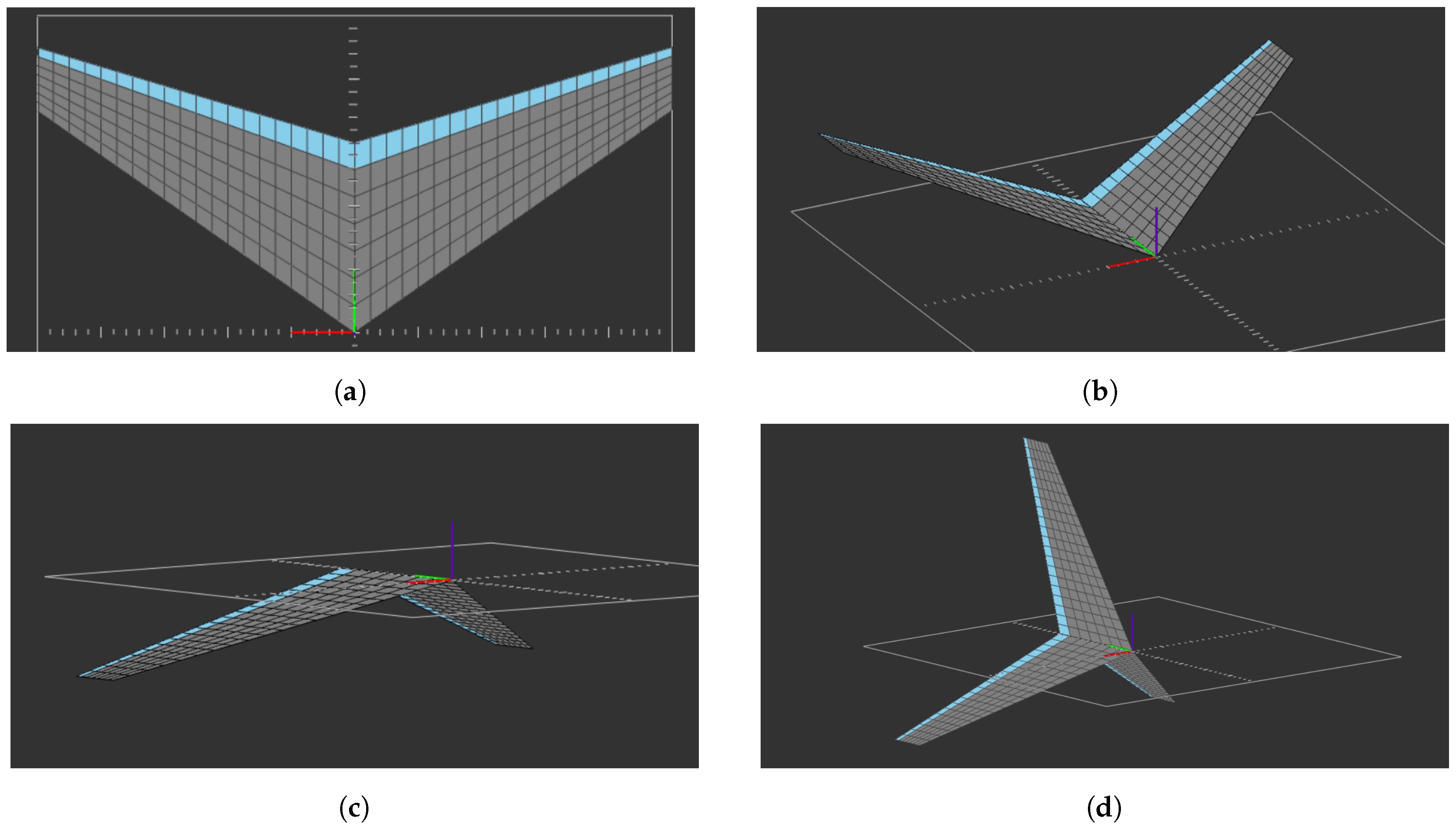
The four considered configurations can be described as follows:
A standard wing with no dihedral angle (
Figure 9a).
A wing with a dihedral angle of 20° (
Figure 9b).
A wing with a dihedral angle of −20° (
Figure 9c).
A set of fins composed of three fins disposed with an angular displacement of 120° between each other (
Figure 9d).
The results presented in the following are obtained considering four test cases for each geometry, with values of the sideslip angle , , , , for a total of 16 simulations. The maximum angle of is chosen to safely fall within the range of application of the model of potential flow on which the software is based. The intensity of the velocity vector was set to 50 m/s and the angle of attack .
Figure 10 shows the results of the analysis, portraying in each plot the outcome of the four experiments carried out on a single configuration. In particular, the plot shows the components of the velocity (red), aerodynamic force (black), and moment (blue) vector lying on the plane normal to
.
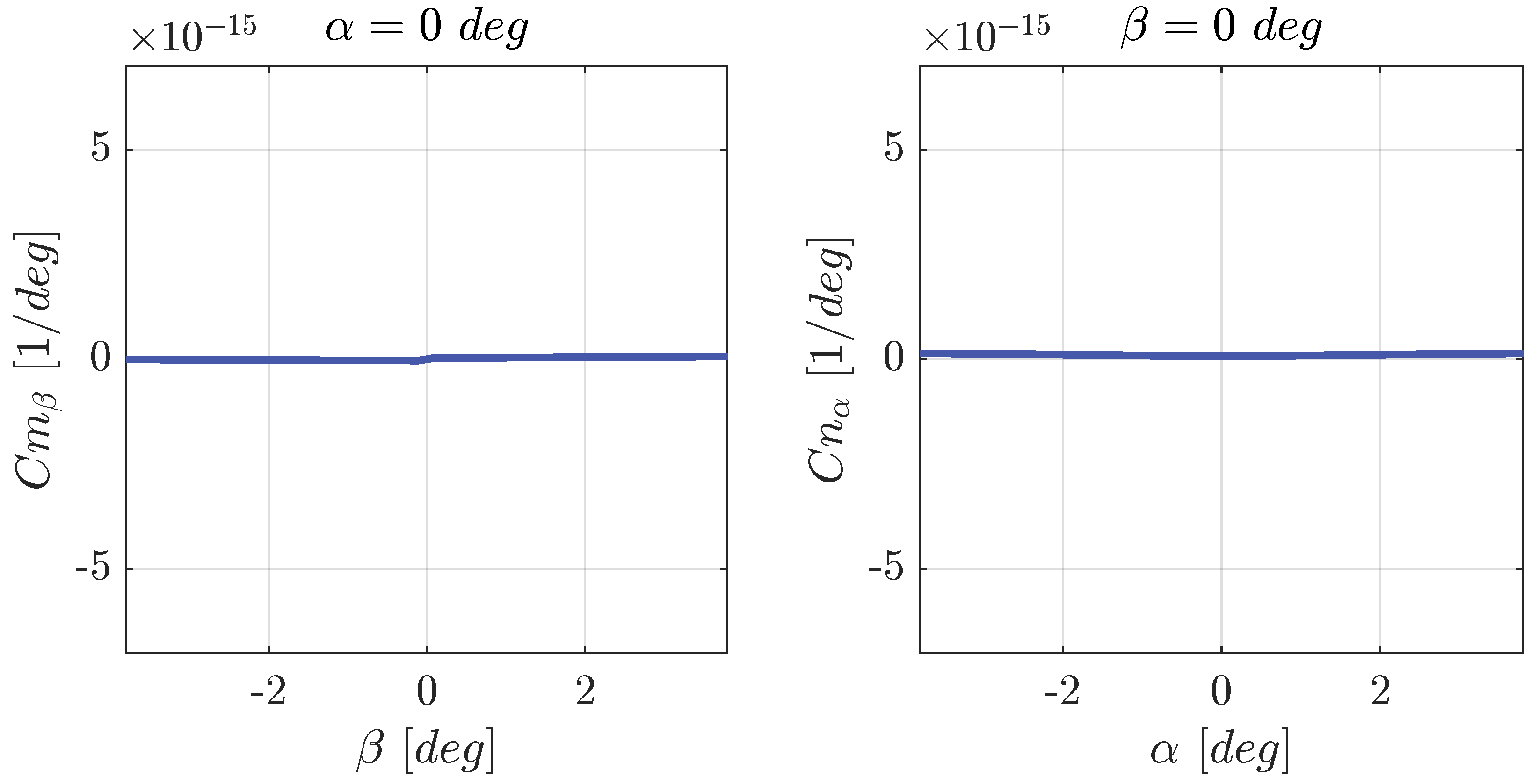
The dihedral layout simulations show that the directions of the force and moment are invariant with respect to the velocity direction. Actually, for this flying wing configuration, most of the aerodynamic force developed lies parallel to the plane of the airfoils (i.e., ), whereas the component not belonging to that plane is comparatively negligible. Therefore, such aerodynamic force can only be effective in counteracting a perturbation on , which is obtained through a corresponding pitching moment. Conversely, the flying wing is not capable of counteracting a perturbation on (and as a consequence, such an aircraft is not statically stable in a directional sense, as known).
On the other hand, for higher absolute dihedral values (i.e., +/−20°), the directions taken by the normal components are correlated with that of the velocity vector.
Finally, for the set of fins, which is of particular relevance since it resembles the fin of a three-finned sounding rocket, a strong coupling with the direction of the velocity vector is similarly obtained.
In order to quantify the ability of a compounded stability index alone to describe the static stability of a system, it is possible to introduce the following parameter
e, which is based on the evaluation of the angle
defined graphically in
Figure 11, and analytically as
Inspecting
Figure 10 and analyzing the value of the parameter
e, it is possible to note that it captures the level of correlation between the normal component of the relative wind velocity and that of the normal force.
In particular, the lower the value of e, the better the correlation. Correspondingly, the significance of the compounded static stability index is increased for lower values of e, meaning that the level of static stability can be employed to better describe the overall (i.e., compounded) level of static stability of the system if the reaction to a perturbation is such as to keep e lower. For example, for the null-dihedral flying wing, the value of e is comparatively high, yielding an inaccurate description of the level of static stability via the compound index, whereas for the set of fins, the parameter e keeps a lower value, and in this case, the compound index of static stability is more descriptive than the two classical indexes for longitudinal and directional stability.
To physically explain this effect, it can be said that the compounded static stability index can be employed to study the static stability of an aircraft when the angle
between the normal component of the total aerodynamic moment and the normal component of the relative wind is sufficiently close to
, for every combination of
and
(which is captured by a corresponding value of
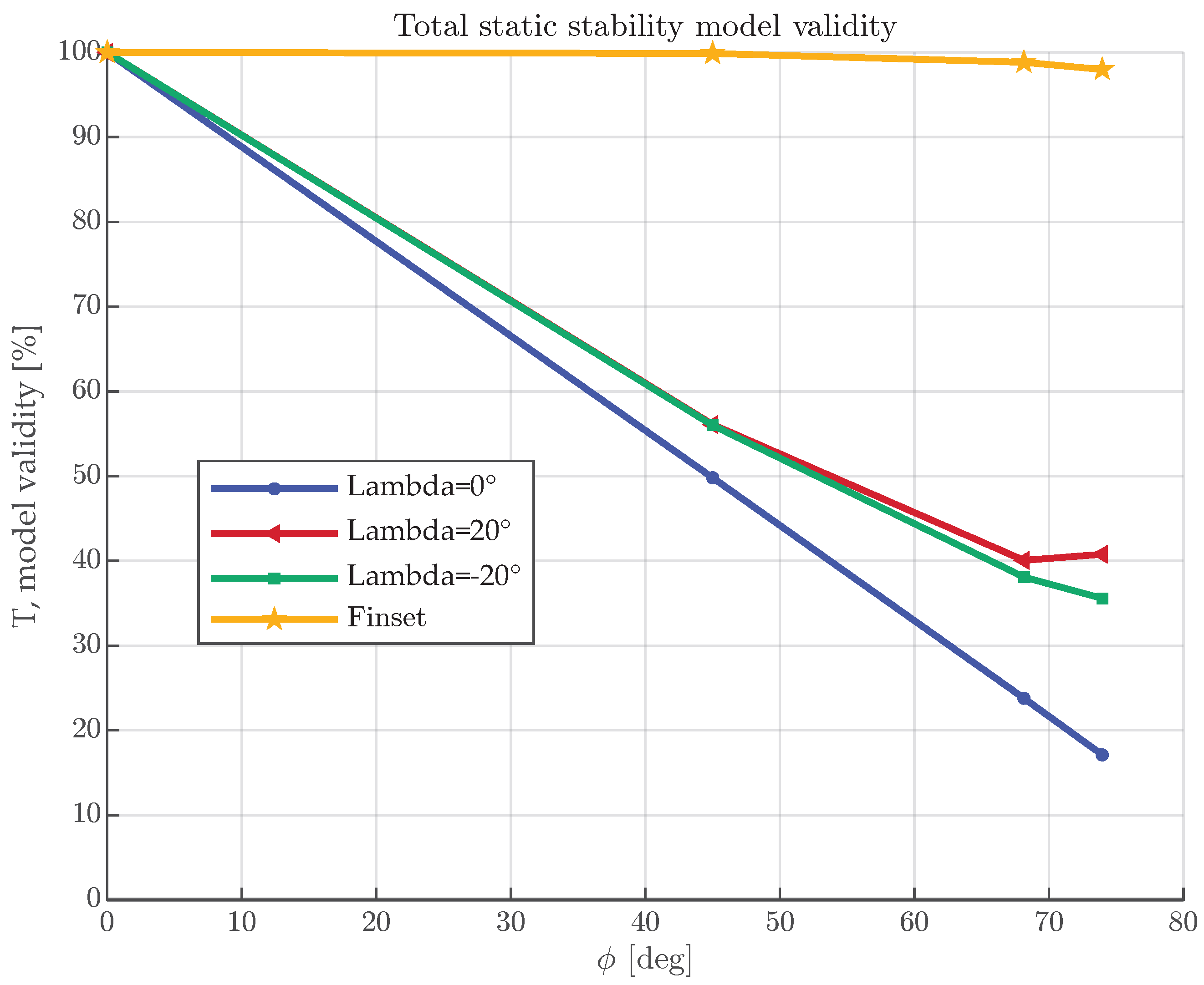
) within a reasonable range. This result is conveniently shown in quantitative terms in
Figure 12, where the parameter
T has been defined as a function of
e only, as
According to its definition, this parameter shall take a higher value for a more reduced level of parameter
e. The plot in
Figure 12, referring to the trials at several values of the angle
considered in the test at hand (which are obtained for the assigned
and
values, where, in particular, only the latter has been changed, as said), shows that for the flying wing at null dihedral, the compounded stability index is descriptive only for
, i.e., when this index is the same as that for the longitudinal static stability. In all other cases, the compound index is poorly descriptive of the level of static stability for this configuration. Substantially similar results are obtained for the flying wing with a positive or negative dihedral. Conversely, for the set of fins, for whatever
, the compounded stability index remains descriptive of the static stability level, whereas the two classical indexes are not, as pointed out in
Section 1 as a problem statement.


