Article

Preliminary Nose Landing Gear Digital Twin for Damage Detection

Department of Mechanical Engineering-Politecnico di Milano, Via La Masa 1, 20156 Milano, Italy
*
Author to whom correspondence should be addressed.
These authors contributed equally to this work.
Aerospace 2024, 11(3), 222; https://doi.org/10.3390/aerospace11030222
Submission received: 7 February 2024 / Revised: 8 March 2024 / Accepted: 11 March 2024 / Published: 12 March 2024
(This article belongs to the Special Issue Aircraft Structural Health Monitoring and Digital Twin)

Abstract

:
An increase in aircraft availability and readiness is one of the most desired characteristics of aircraft fleets. Unforeseen failures cause additional expenses and are particularly critical when thinking about combat jets and Unmanned Aerial Vehicles (UAVs). For instance, these systems are used under extreme conditions, and there can be situations where standard maintenance procedures are impractical or unfeasible. Thus, it is important to develop a Health and Usage Monitoring System (HUMS) that relies on diagnostic and prognostic algorithms to minimise maintenance downtime, improve safety and availability, and reduce maintenance costs. In particular, within the realm of aircraft structures, landing gear emerges as one of the most intricate systems, comprising several elements, such as actuators, shock absorbers, and structural components. Therefore, this work aims to develop a preliminary digital twin of a nose landing gear and implement diagnostic algorithms within the framework of the Health and Usage Monitoring System (HUMS). In this context, a digital twin can be used to build a database of signals acquired under healthy and faulty conditions on which damage detection algorithms can be implemented and tested. In particular, two algorithms have been implemented: the first is based on the Root-Mean-Square Error (RMSE), while the second relies on the Mahalanobis distance (MD). The algorithms were tested for three nose landing gear subsystems, namely, the steering system, the retraction/extraction system, and the oleo-pneumatic shock absorber. A comparison is made between the two algorithms using the ROC curve and accuracy, assuming equal weight for missed detections and false alarms. The algorithm that uses the Mahalanobis distance demonstrated superior performance, with a lower false alarm rate and higher accuracy compared to the other algorithm.

1. Introduction

An increase in aircraft availability is one of the most desired characteristics of aircraft fleets. Delays due to unforeseen failures cause additional expenses, especially when they occur without adequate maintenance staff and equipment. This is particularly critical since a proper supply chain is known to improve aircraft availability [1]. Therefore, researchers have focussed their attention on technologies that could help detect incipient failures and assist in decision-making and problem solving due to these unfortunate events. However, the common practice in companies is the use of Key Performance Indicators (KPIs) to identify the root causes of downtime, predict future trends in service reliability, and select maintenance solutions with the best impacts on aircraft availability [2].
For instance, combat jets and Unmanned Aerial Vehicles (UAVs), in particular, are used in extreme conditions, and there can be situations where standard maintenance procedures are impractical or unfeasible, such as when aircraft operate from a temporary airfield, when maintenance time might be limited. The readiness rate for military aircraft is a current concern of national air forces [3,4], as it also reflects the efficiency of maintenance practices, among other factors.
Therefore, it is important to develop condition-monitoring and diagnostic algorithms that minimise maintenance downtime [5], improve safety, and reduce maintenance costs. This highlights the possibility of designing a Health and Usage Monitoring System (HUMS). A HUMS consists of algorithms that must analyse signals in real time to provide both a diagnosis and a prognosis, that is, the estimation of residual useful life (RUL), to support decision-making using damage indicators selected ad hoc for the application. In this framework, digital twins can be used to mimic the behaviour of real systems [6], providing information on the performance of the system to allow effective maintenance and operation planning.
Focussing on the aviation industry, digital twins provide a virtual representation of systems, such as aircraft, or some of their subsystems of critical interest, such as engines, landing gears, and others. In particular, among the several subsystems into which aircraft can be divided, landing gears are one of the most complex systems, as they include a wide range of elements, including actuators, shock absorbers, and flexible structures, since they span various physical domains. Recent studies have pushed towards alternative designs [7] and the structural monitoring of nose landing gears [8,9] and their bays [10,11,12], for instance, with strain gauges and fibre Bragg grating techniques. However, the monitoring of the nonstructural aspects of the nose landing gear, for instance, to ensure proper functioning, rather than predicting its residual fatigue life, has not been widely investigated.
Therefore, this work aims to model a preliminary digital twin of a nose landing gear in the MATLAB®-Simulink® environment within the HUMS framework. The concept of the preliminary digital twin is used due to the lack of real-time update capabilities of the nose landing gear model parameters, which is one of the requirements of a digital twin [13]. However, the choice of the modelling environment has been made since the Simulink® tool allows for multiphysics block-based modelling that, together with the MATLAB Simscape Multibody library, provides a holistic framework for capturing interactions among the different physical domains of complex systems, such as a nose landing gear. In particular, Simscape libraries allow for the possibility of artificially injecting damages to replicate the system’s behaviour in anomalous conditions. This means that the preliminary digital twin developed can be used to mimic the behaviour of the real system under healthy conditions, but, by implementing damage models in it, it is also possible to represent the anomalous operations of the real system. Eventually, a database can be obtained that collects signals from healthy and damaged simulations and can be used to develop machine learning algorithms that can be used for the HUMS application. This enhances the comprehension of the effects of damage on the entire system and the explainability of damage detection algorithms since they will be generated and tested on a multiphysics database.
Therefore, this work aims to demonstrate the use of digital twins for designing HUMS and damage detection algorithms by generating databases of signals acquired under healthy and faulty conditions. A framework is proposed to compare different algorithms and support the choice of the algorithm to implement, accounting for the relative perception of missed detections and false alarms.
The detection of anomalies in the HUMS framework is usually carried out by performing an outlier analysis [14,15,16,17], as the aim of the algorithms is to detect deviations from the designed behaviour in the presence of new unknown data and because, often, damage data are not available. In particular, two damage detection algorithms are going to be compared in three anomalous scenarios: the first algorithm is based on the RMSE, while the second relies on the Mahalanobis distance. The RMSE-based method is less sophisticated than the Mahalanobis distance-based one and does not consider the correlation characteristic between signals. Nevertheless, it is a simpler and easier-to-implement alternative. Therefore, it is interesting to compare its performance with a more complex method, such as the Mahalanobis distance.
Finally, the choice of the algorithm to implement for the real system can be based on the Receiver Operating Characteristic (ROC) curve [18], that is, a plot of the probability of detection (POD) versus the false alarm rate (FAR). However, to take into account how a false alarm is considered with respect to a missed detection, a weighted accuracy is proposed to perform a trade-off between the POD and FAR, which, for example, can be based on the potential cost of having a false alarm rather than a missed detection.

2. Damage Detection Algorithms

Within the HUMS framework, diagnostic algorithms play a crucial role in detecting anomalies [19]. These algorithms must identify when the behaviour of the system deviates from the expected behaviour, which is called the baseline and represents the system under healthy conditions. Depending on the degree of difference observed, the algorithms should indicate whether the system needs to be serviced soon or whether it should be serviced immediately. This study proposes two diagnostic algorithms for the nose landing gear application; the first is based on the Root-Mean-Square Error (RMSE), while the second relies on the Mahalanobis distance (MD). It is important to note that the performance of a diagnostic algorithm depends on the specific characteristics of the system being monitored and the type of fault.

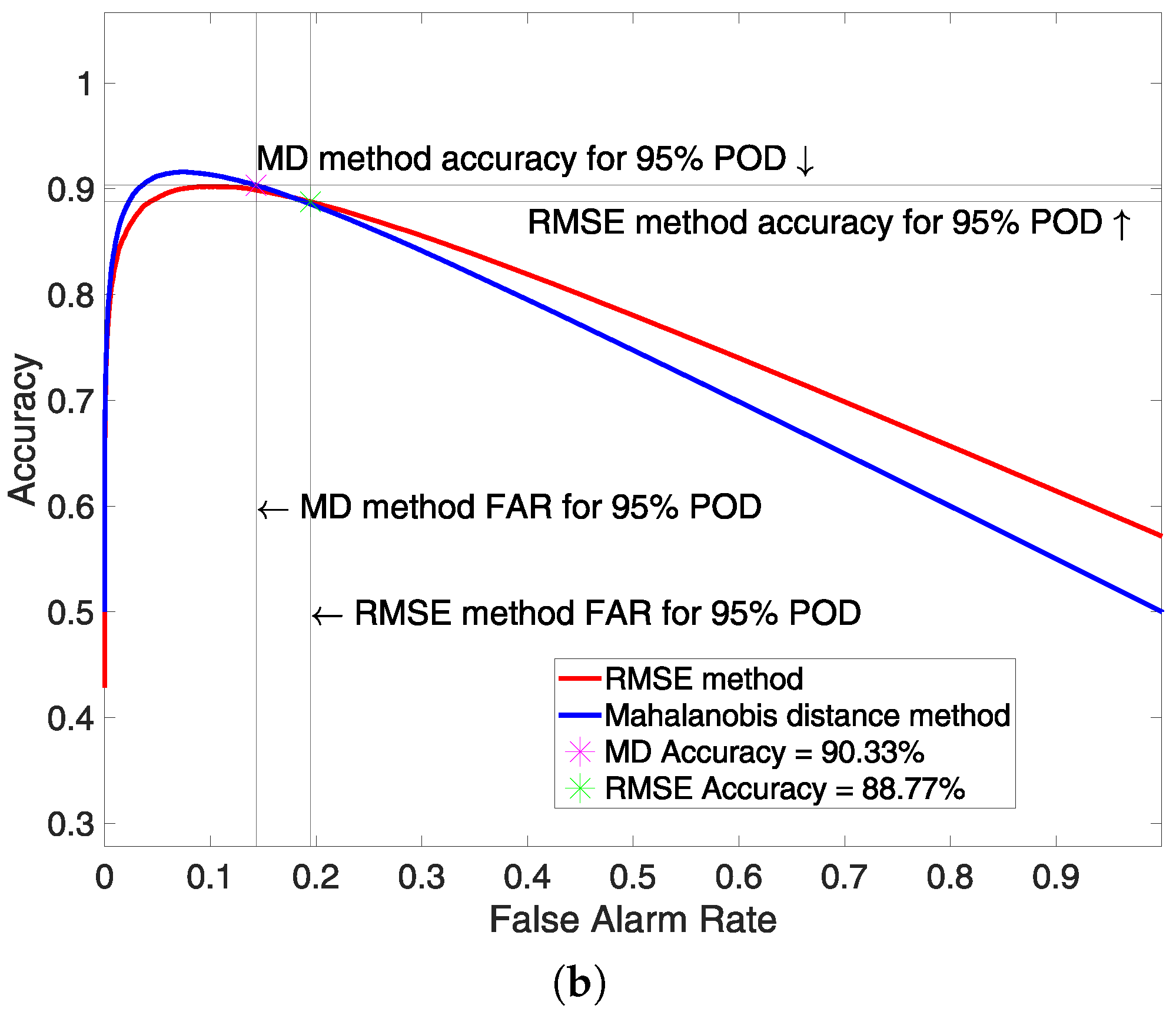
2.1. Diagnostic Algorithm Based on RMSE

The Root-Mean-Square Error is commonly used to evaluate the quality of predictions and indicates how far the predicted values fall from the actual measured values using the Euclidean distance. This Euclidean distance can be used to measure the distance of a faulty signal from the baseline. The RMSE-based diagnostic algorithm involves the following steps:
  • Calculate the RMSE E between the measured signals and the baseline.
  • Define a threshold E * for E based on the baseline statistics.
  • If E > E * , the system is declared damaged.

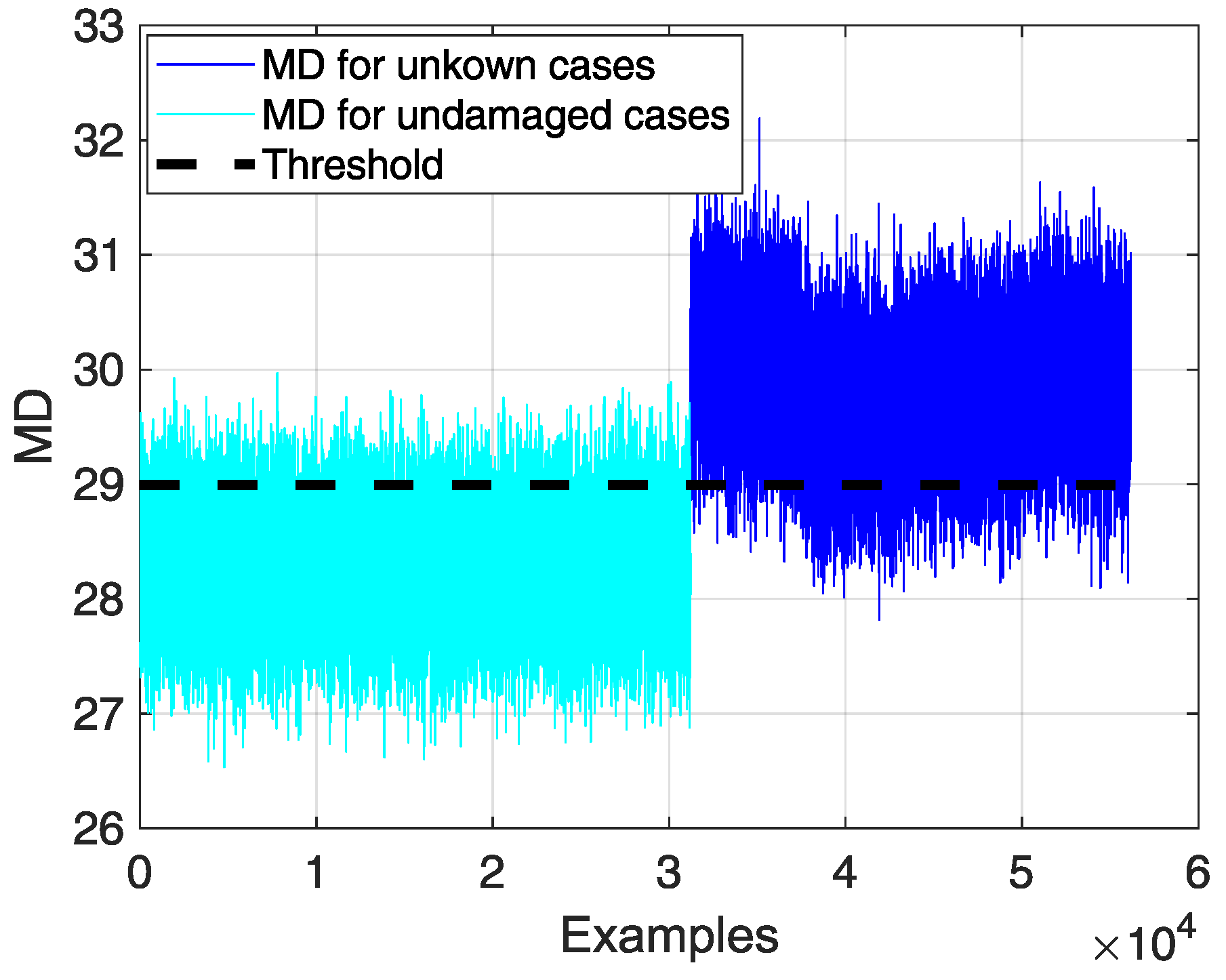
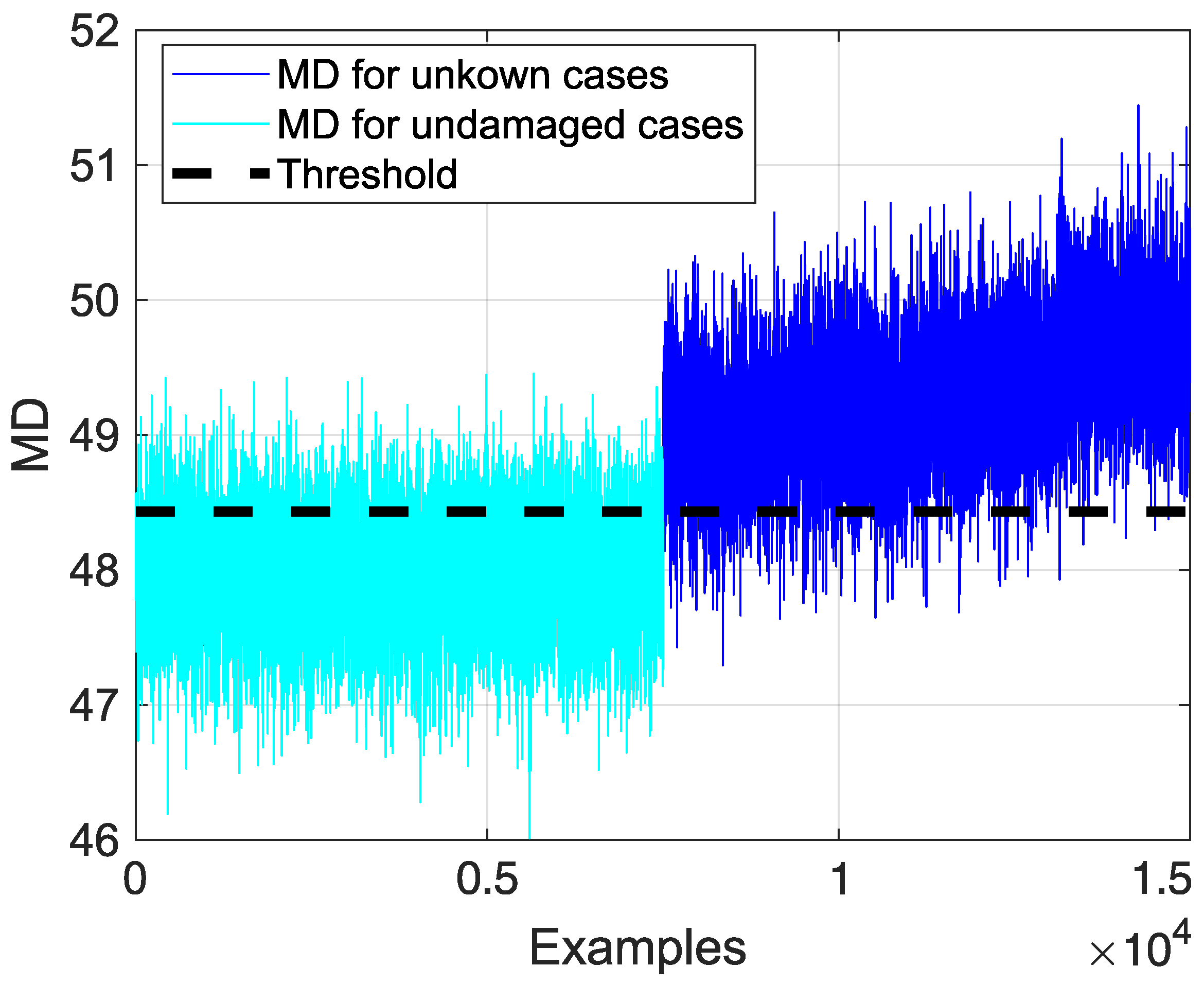
2.2. Diagnostic Algorithm Based on Mahalanobis Distance

The Mahalanobis distance is usually used in statistics for multivariate outlier analysis. It determines whether a point belongs to a cluster or is considered an outlier. The Mahalanobis distance is a weighted Euclidean distance [20], with the weight function being the inverse of the covariance matrix of the cluster. This method takes into account the correlation characteristics between the elements in the clusters [21].
In the HUMS and Structural Health Monitoring (SHM) framework, the Mahalanobis distance from a healthy cluster, that is, the baseline, is used to determine whether the system under analysis has any damage [22,23,24,25,26,27].
This approach allows one to calculate the statistical distance of a vector with n measured values x ¯ = [ x 1 ; x 2 ; . . . ; x n ] R 1 x n from a multivariate Gaussian distribution with a mean vector μ ¯ x = [ μ x , 1 ; μ x , 2 ; . . . ; μ x , n ] R 1 x n and a covariance matrix S R n x n as follows:
M D ( t ) = ( x ¯ ( t ) μ ¯ x ) T S 1 ( x ¯ ( t ) μ ¯ x )
where μ ¯ x and S represent the baseline. The steps for the implementation of diagnostic algorithms based on the Mahalanobis distance are the following:
  • Compute the mean vector μ ¯ x and the covariance matrix S for the healthy baseline condition.
  • Define a threshold M D * for M D based on the baseline statistics.
  • Compute M D ( t ) for the observation x ¯ ( t ) , measured at time t.
  • If M D ( t ) > M D * , the system is declared damaged.

3. Nose Landing Gear Digital Twin

The Computer-Aided Design (CAD) assembly of the nose landing gear was imported into Simulink thanks to the Simscape Multibody tool. The components within the 3D assembly are treated as rigid bodies, accounting for mass and inertia properties similar to the real physical parts. These bodies are interconnected through Multibody joints that mimic the actual connections to replicate the behaviour of the real system.

3.1. The Oleo-Pneumatic Shock Absorber

The landing gear system absorbs and dissipates the kinetic energy of the aircraft during the landing phase, dampening the impact and transferring lower loads to the rest of the airframe through a shock absorber. The shock absorber implemented is oleo-pneumatic and can be divided into two parts: a nitrogen chamber (represented in blue in Figure 1) and an oil chamber. The latter consists of two parts: a primary part (depicted in yellow in Figure 1), also called the orifice support because it has an orifice attached, and a secondary part (in purple in Figure 1), known as the metering pin support, because it houses a metering pin. When the shock absorber is compressed, the metering pin, which is represented in grey in Figure 1, reduces the area of the orifice available for oil exchange between the two chambers, ensuring that the desired load–stroke pattern is achieved. Figure 1 shows a schematic of the oleo-pneumatic shock absorber, where x is the inertial reference position, A f p and p g a s are the area and pressure of the nitrogen chamber, respectively, while A o and p o 2 are, respectively, the area in the support extremity of the orifice and the pressure inside the secondary part of the oil chamber, q is the flow between the primary part and the secondary part of the oil chamber, and F f is the friction force in the sealings between the two concentric cylinders.
The equation of motion of the shock absorber, according to [5], is
M x ¨ = M g p g a s A f p p o 2 A o F f
where M denotes the total mass of the moving components of the shock absorber, g is the acceleration due to gravity, and the other terms are the ones described regarding Figure 1. The flow inside the primary and secondary parts of the oil volume is simulated according to the following equations, described in [28]:
q = d d t ρ V ρ l 0 = d d t ρ ρ l 0 V + ρ ρ l 0 · ϵ · ( v R v C ) · A
F f = p · A
where q is the flow rate to the converter chamber, A is the effective piston area, v R is the converter rod velocity, v C is the converter case velocity, F is the force developed by the converter, p is the gauge pressure of fluid in the converter chamber, V is the piston volume, and ρ l 0 is the fluid density at atmospheric conditions. Since the compressibility effects of the oil are considered relevant, the density of the oil is related to its pressure through the bulk modulus, the specific heat ratio, and the relative amount of trapped air. Notice that the temperature of the oil is almost constant during compression [5]. The flow equation envelopes an energy equilibrium that involves the internal energy of the fluid and the mechanical energy given by the variation in the volume of the chamber over time.
As regards the nitrogen volume, the mass and energy balance is explicitly defined as follows:
M p · d p I d t + M T · d T I d t + ρ I · d V d t = m I ˙
where M p is the partial derivative of the mass of the gas volume with respect to pressure at constant temperature and volume, M T is the partial derivative of the mass of the gas volume with respect to temperature at constant pressure and volume, p I is the pressure of the gas volume, T I is the temperature of the gas volume, ρ I is the density of the gas volume, V is the volume of gas, t is time, and m I ˙ is the mass flow rate. The subscript “I” means that they are quantities interfaced through the ports of the block to the rest of the Simscape network. The term ρ I · d V d t is related to the change in gas volume and therefore to mechanical movement. Energy conservation relates the energy and heat flow rates to the dynamics of the pressure and temperature of the gas volume:
U p · d p I d t + U T · d T I d t + ρ I h I d V d t = Φ I + Q I
where U p is the partial derivative of the internal energy of the gas volume with respect to pressure at constant temperature and volume, U T is the partial derivative of the internal energy of the gas volume with respect to temperature at constant pressure and volume, Φ I is the energy flow rate, Q I is the heat flow rate, and h I is the specific enthalpy of the gas volume.
The partial derivatives of the mass M and the internal energy U of the gas volume with respect to pressure and temperature in a constant volume depend on the gas property model. For a perfect gas model, the equations are as follows:
M p = V ρ I β I
M T = V ρ I α I
U p = V ( ρ I h I β I T I α I )
U T = V ρ I ( c p I h I α I )
where β is the isothermal bulk modulus of the gas volume, and α is the isobaric thermal expansion coefficient of the gas volume.
The properties of nitrogen, modelled as a perfect gas, and oil, modelled as an isothermal fluid, have been hypothesised from engineering websites [29] and Simulink’s pre-existing oil models that are built into the Hydraulic Fluid block [30] used. The assumed initial pressure within the chambers is in the range of a few bars, in line with the typical values found in the literature on oleo-pneumatic struts [5,31].
The reduction in the available orifice cross-section with stroke, described in relation to Figure 1, was modelled by a Needle Valve block, where the flow rate through the orifice is proportional to the opening of the orifice and the pressure differential across the valve. The flow rate is determined according to the following equation:
q = C D · A ( h ) 2 ρ Δ p ( Δ p 2 + p C r 2 ) 1 / 4
where q is the flow rate through the orifice; Δ p is the pressure difference between the primary and secondary parts of the oil chamber; C D is the flow discharge coefficient; A ( h ) is the instantaneous orifice passage area, which changes with h, that is, the valve opening, and takes into account the conical shape of the metering pin; and p C r is the minimum pressure for turbulent flow, which is calculated from the critical Reynolds number, found to be approximately 10 from the literature on the valves [32].
However, representing the metering pin as a valve in the model neglects the influence of forces on the surface of the metering pin. To address this, a force is applied to the metering pin support, acting oppositely to the direction of motion, and it is calculated as the absolute value of the pressure in the primary part of the oil chamber multiplied by the area of the head of the metering pin, as reported in Equation (12):
| F | = | p o 1 | A m p h
The friction forces in a conventional damper depend on the operating conditions. The pressure that pushes the seal against the wall of the cylinder may be known, but the lubrication conditions between the sealing ring and the cylinder are uncertain. The friction force due to the contact between the moving components can be seen as composed of two parts: a static force and a viscous term. The static force F s , also called the Coulomb force [33], is constant regardless of the velocity, while the viscous force F v opposes motion and scales directly with the relative velocity.
An estimation of the normal force between a piston ring and a cylinder can be calculated from [32]
F N = 1 2 A s Δ p
where Δ p is the pressure acting on the seal, A s is the seal outer surface area A s = π D p L s , D p is the external diameter of the piston, and L s is the seal ring axial length. Around both the floating piston and the cylinder that contains the primary part of the oil chamber, there are two seals placed in series, so the area considered is doubled, and, moreover, the presence of PTFE, also known as Teflon, has been hypothesised for an estimation of the Coulomb friction coefficient μ M , giving the static piston friction force:
F s = μ M F N
In the model, the static force is taken into account by subtracting these friction forces, obtained as explained, and the ones acting on the Multibody joints. Instead, viscous forces are considered by modifying the internal mechanics of the joints, thus adding a damping coefficient.

3.2. The Steering System

The nose wheel steering system plays a critical role during the landing process, ensuring precise control for taxiing along the runway. Traditionally, hydraulic systems have been predominantly used for this system; however, there is a growing shift towards electric systems for future More/All-Electric Aircraft. This transition aims to eliminate issues such as hydraulic leakage and optimise space and weight, ultimately enhancing the reliability and ease of maintenance of these systems [34].
In the UAV (Unmanned Aerial Vehicle) under analysis, the nose wheel steering system is electromechanical, composed of a brushless DC motor and a speed reducer, together with a steering controller and an angular displacement sensor. When avionics commands are received, the steering controller activates the electric motor. Its rotation is reduced by a gear reducer inside the steering drive mechanism. This mechanism is linked to the wheel via a series of linkage mechanisms, enabling the wheel’s steering movement.
The controller was modelled in a Simscape environment as a PI controller.In the development of the preliminary digital twin for the nose landing gear, the Motor & Drive block serves as a simplified but effective model of the brushless DC motor. It represents a generic DC motor and drive with closed-loop torque control. To enable fast simulation at the system level, this block abstracts the motor, the drive electronics, and the control.
The torque–speed envelope profile is determined by specifying the maximum torque and power [35]; these values have been estimated from similar systems [36]. The motor is driven by an ideal voltage source that maintains constant voltage across its output terminals, independent of the current flowing through the source, simulating the batteries used in a real vehicle.
The torque generated by the Motor & Drive block passes through a Gear Box block, which amplifies the torque, reducing the angular velocity. The Multibody Revolution joint block allows for one rotational degree of freedom. This joint is actuated by the output torque of the Gear Box block and senses the rotation of the linkage mechanism. The rotation signal is then fed to the PI controller, which computes the error by comparing the rotation signal with the received steering signal, generating the target torque to be produced by the motor. The PI controller was tuned using the Simulink PID tuner tool. To replicate the effect of the friction of the joints in operational activities, the Rotational Friction block is used to provide resistance torque and dampen the rotation. Hence, the Simscape mechanical network described is linked to the Multibody joint. During the simulation, the motor current and angle-of-rotation signals are sensed. These will then be instrumental in assessing the state of the steering system in Section 6.

3.3. The Retraction/Extraction System

The landing gear retraction/extraction system of an aircraft is one of the critical systems of the aircraft. The overall speed and flight performance improve after taking off when the landing gear is correctly retracted. Similarly, the landing gear system must be extended properly to ensure a safe landing.
The actuator responsible for the extraction and retraction of the nose landing gear is electromechanical. It is equipped with a drive mechanism that reduces the high-speed rotational motion by increasing the torque. The latter is then used to turn a screwdriver, resulting in the linear motion of the acme drive nut. A downlock mechanism is used to keep the landing gear retracted. This mechanism is disengaged when landing gear extraction is required. In Simscape, the retraction/extraction system was modelled similarly to the nose wheel steering system. A Motor & Drive block represents the actuator, which is connected to a Gear Box block that mimics the drive mechanism, reducing the speed by increasing the torque. The latter becomes the input of a Leadscrew block that converts the rotational motion into a linear one. The Leadscrew block represents a threaded rotational–translational gear that constrains the two connected driveline axes, i.e., the screw and nut, to, respectively, rotate and translate together in a fixed ratio. L is the translational displacement of the nut for one screw turn and is a parameter that relates the angular velocity of the screw and the translational velocity of the nut:
ω S L = 2 π v N
The linear motion is sensed, and it is used by the modelled PI controller to compute the error against the target signal received. Therefore, the controller computes the target torque that should be produced by the motor. Ultimately, in the Multibody domain, the resulting force actuates the joint responsible for the motion, closing or opening the landing gear. A Multibody joint is used to mimic the downlock mechanism and is able to either hold the landing gear in its position (retracted/extracted) or allow the motion. Analogously to the nose wheel steering system, the motor is driven by an ideal voltage source, whose current is logged for monitoring reasons. To account for the friction and damping of the joints responsible for the retraction movement, the Multibody joints used are characterised by high friction and damping coefficients.
The PI controller was tuned using the Ziegler–Nichols method. The voltage and reduction ratio values of the gearbox were estimated from [37].

4. Case Studies and Model Comparative Analysis

Three different scenarios have been identified as the most representative case studies of interest for a nose landing gear:
  • Nose wheel steering system simulation;
  • Retraction/extraction system simulation;
  • Aircraft landing simulation.
In the first scenario, the landing gear is fully extended, and a step signal is applied to the PI controller of the steering system, causing the nose wheel to rotate to the desired angle. This simulates the turn of the aircraft during taxing operations. In the second case study, the nose wheel is kept in a straight position, and a step signal corresponding to a retraction command is input into the PI controller of the retraction system. Consequently, the landing gear retracts. After a 2-s interval, the reverse step signal is applied to the previous one, initiating the extraction of the landing gear. The last scenario is realised by keeping the landing gear extended and applying a vertical force to the wheel, simulating a landing. To determine the magnitude of the force, reference [38] specifies the use of 15% of the weight on the nose landing gear under normal conditions. The weight of the system under analysis was from an aircraft with a similar wingspan [39].
These three case studies allow for the comparison of the developed digital twin performance with literature references to check whether the implemented models follow realistic behaviours. In particular, the following characteristics are selected since these signals capture the behaviour of the nose landing gear:
  • The current feeding the motor and the torque and angular velocity of the actuator for the steering system.
  • The current that feeds the motor, force, and the stroke of the actuator for the retraction/extraction system.
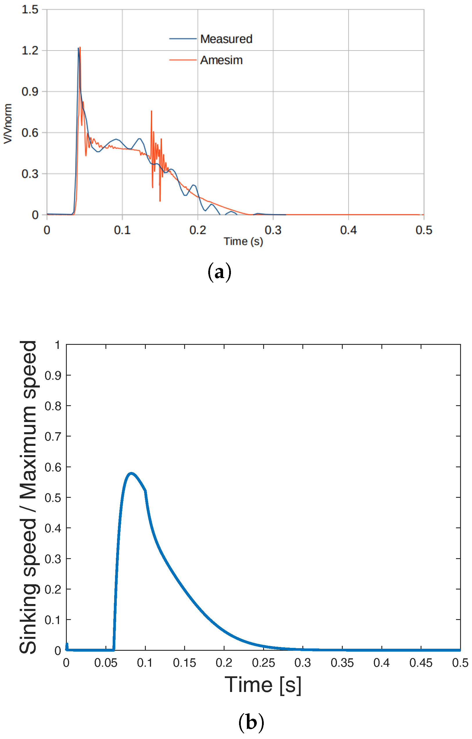
  • The pressure of the shock absorber chambers, stroke, and the sinking speed of the shock absorber to land the aircraft.
An exact validation of the models is currently unattainable, as the nose landing gear manufacturer cannot disclose the data. However, if the models in each simulation behave correctly and the results are comparable to relevant references, the models can be useful in this preliminary phase. As more data are disclosed about the real physical model, there is the possibility that their virtual counterparts can be modified, moving towards a more robust validation.

4.1. The Steering System

The modelled steering system effectively rotates the wheel to the specified angles given as input to the PI controller, achieving the desired position in approximately 1 s. Furthermore, the landing gear manufacturer supplied essential actuator details, such as the actuator stall torque, which represents the torque produced when the output rotation speed is zero [40], and the no-load speed, which denotes the maximum speed at which the output shaft can rotate when there is no load on the motor [41]. These are compared with the maximum torque and maximum angular velocity generated by the rotative actuator modelled in Simscape in Section 3.2. The comparison is made using safety factors to avoid the disclosure of sensitive information, as shown in Table 1.

4.2. The Retraction/Extraction System

The retraction/extraction system makes the nose landing gear retract, and after a couple of seconds, it is extracted to return to an extended position. The duration of the retraction phase is close to the one discussed in [38].
Again, in this case, basic actuator specifics were shared, including the maximum force exerted and the maximum stroke of the linear actuator. These are compared with the maximum force and the maximum stroke recorded during the nose landing gear extraction case study in Table 2. In this scenario, almost the entire available stroke is used because, otherwise, the landing gear would not retract. The actuator moves slowly and in a controlled manner. Additionally, an electrical switch is employed to automatically stop the process, ensuring safe operation.

4.3. The Oleo-Pneumatic Shock Absorber

Concerning the last scenario, a simulation was carried out to replicate the case explained in [5], which is known as the dynamic case. In reference [5], a comparable oleo-pneumatic shock absorber is modelled for a military aircraft with a similar internal architecture. It also incorporates a metering pin that reduces the area of the orifice between the two parts of the oil chamber, which is used to dampen the compression. The main difference is in the gas chamber configuration, which features a parallel gas chamber with significantly higher pressure. This parallel chamber engages in the last stage of the compression stroke to cushion the impact. Instead, in this work, the gas chamber is in series with the oil chamber. Despite this difference in configuration, the expected behaviour should be consistent between the two, with the compression process effectively dampened.
The model used as a reference [5] has been validated with experimental data, and, therefore, a comparison with the results of the model implemented in this work is of great interest. In the Simscape model of the nose landing gear implemented in this work, a force signal was reproduced to follow the one used in [5]. The maximum value was estimated as discussed in Section 3.1.
This force was applied to the Multibody solid block of the wheel, connected to the rest of the landing gear.
The position and velocity between the cylinder attached to the rest of the aircraft and the cylinder that slides inside it are recorded. The Multibody joint between them is exploited to sense these quantities. These represent the stroke and sinking speed of the shock absorber. Therefore, the simulation results are compared with the results of [5] in Figure 2 and Figure 3.
Looking at Figure 2, it must be stated that the normalisation scale used in this work (Figure 2b) is different from the one in [5] (Figure 2a). However, the comparison shows that the model implemented is able to represent the real behaviour, as the time required for complete motion damping is around 0.3 s in both cases. The difference in velocity profiles shown in the pictures is due to the different shock absorber designs since, in this work, the gas chamber is in series with the oil chamber, while they are in parallel in the reference used.
The stroke of the shock absorbers is compared in Figure 3. Similarly to what was observed for the sinking speed, Figure 3a,b have a similar shape and, in this case as well, the normalisation scales used in the two plots are different. The model used as a reference suffered from noise due to the high intensity of forces and the freeplay considered in the assembly of the landing gear.
A final comparison is made by analysing reference values for the shock absorber used to design the nose landing gear. The landing gear manufacturer supplied data on the maximum sinking speed and stroke of the shock absorber. Reaching the maximum stroke implies contact between parts of the shock absorber, which can cause the wear of steel components, such as the upper cylinder and the base connected to the wheel. These data are compared with the maximum sinking speed and stroke values measured during the simulation described previously, and the safety factors are calculated and listed in Table 3.

5. Damage Implementation

Within the HUMS framework, the developed digital twin can be used to design and test diagnostic algorithms, using the signals obtained during simulations as a database. It becomes imperative to formulate a condition-monitoring and fault detection algorithm, particularly for critical components such as landing gears. In this section, damages that may occur during routine aircraft operations were modelled in the Simulink environment. Three types of damage were introduced, each in one of the aforementioned case studies:
  • Wear (severe damage) and dirt accumulation (mild damage) in the bearings devoted to steering.
  • Wear (severe damage) and dirt accumulation (mild damage) in the bearings used for the extraction/retraction movement.
  • Leakage of the oil chamber.
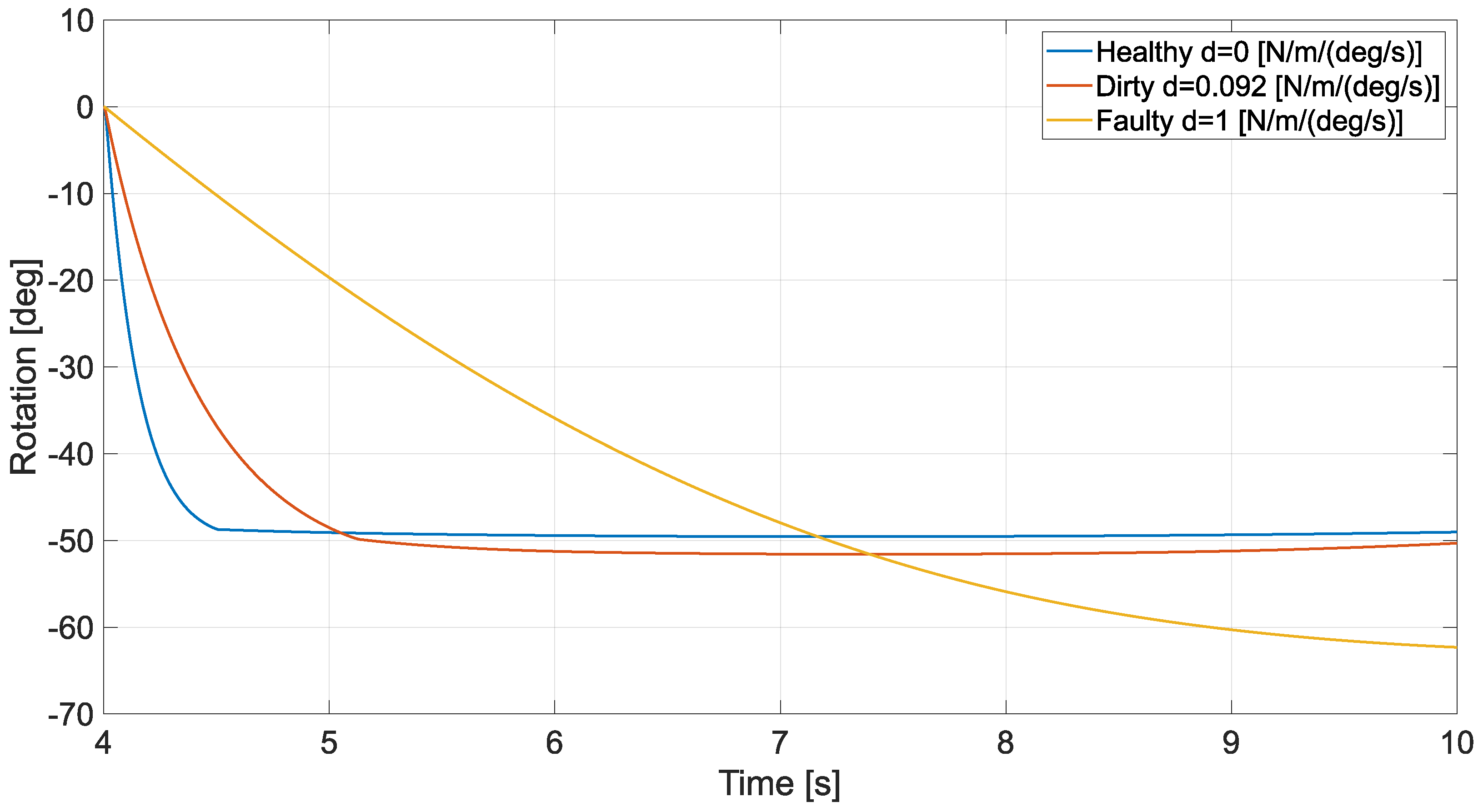
In general, Simscape allows for the modelling of many types of faults within a system. In addition, the temperature inside the chambers of the shock absorbers could be initialised at very low or high values to simulate operations under extreme weather conditions, which would change the performance of the shock absorber.

5.1. Bearing Wear

Bearings are essential mechanical components that experience a decrease in performance during flight hours due to the accumulation of different types of dirt, such as dust, solidified grease, and other external contaminants. This accumulation prevents smooth rotation, affecting not only conventional rolling bearings but also plain bearings. It is interesting to observe the response of the system to the same input with different values of the bearing damping coefficient. In a dirty condition, a bearing is considered to have a certain damping coefficient, which is greater than the value given by the datasheets. Under faulty conditions, the rotation could be further dampened, resulting in a higher damping coefficient. Coefficients greater than 0.092 N/m/(deg/s) are associated with a worn bearing [42,43]. Therefore, the damping coefficient is assumed to be
  • 0 N/m/(deg/s) in the healthy case.
  • 0.092 N/m/(deg/s) in the dirty scenario.
  • 1 N/m/(deg/s) in the faulty condition.

5.1.1. The Steering System

This section addresses the scenario in which one of the bearings that allows steering has modified internal mechanics leading to higher damping coefficients than under normal conditions. Multiple simulations were executed, during which the rotation signal was recorded. To capture changes in the system response, a rotation sensor is used for the steering mechanism in the electrical actuator. To analyse the differences in system responses between damaged and undamaged conditions, the signals are plotted and reported in Figure 4. In all the cases reported, steering starts with a straight wheel, and then a step signal is provided to the PI controller, which activates the motion. As can be observed in Figure 4, the blue line, representing the healthy case, takes less than 5 s to carry out the imposed steering. In contrast, the red and yellow lines, associated with dirty and faulty bearings, respectively, are not able to reach the desired rotation in the simulation time. In particular, the faulty system (in red) takes too long to turn the wheel, which is a damage indicator for the bearings responsible for the rotation of the wheel.

5.1.2. The Retraction/Extraction System

This section focusses on the case in which the bearings devoted to allowing the extraction/retraction movement are subjected to mild and severe damages. Therefore, as explained before, higher damping coefficients are used with respect to healthy conditions.
The sensor of the nut position in the linear electrical actuator is used to capture changes in the system response. The actuator extends until the stroke approaches its maximum normalised value of 1, retracting the nose landing gear. After reaching its fully retracted position, it returns to its fully extracted position. The retraction phase is the most critical for the actuator, as it must overcome gravitational forces. A mildly faulty case is found for a damping coefficient of 0.092 N/m/(deg/s). The retraction/extraction system is less sensitive to changes in system characteristics, as shown by the system response in Figure 5 for the retraction of the landing gear. Looking at this figure, one can notice that the healthy and mildly damaged cases, represented in blue and red, respectively, almost overlap. The severe damage scenario, depicted in yellow, deviates significantly from the healthy response. The extraction is not presented in Figure 5 for the sake of brevity.

5.2. Seal Leakage

In normal operations, planned inspections are performed to ensure the integrity of the shock absorber [5], but these are not sufficient in the event of unexpected events, such as hard landings. During hard landings, there is a risk that the sinking speed specified by the shock absorber manufacturer could be exceeded, generating excessive pressure within the chambers. This pressure might cause the plastic deformation of the chamber walls, leading to an increase in the internal volume of the cylinders. This deformation could also cause misalignment between the larger and smaller cylinders, potentially contributing to oil leakage. When oil leaks from the chamber, the pressure inside both chambers decreases, compromising the impact cushioning capability. Consequently, a leakage in the seal around the smaller sliding cylinder was modelled in Simscape by introducing a Fixed Orifice block into the hydraulic network of the oil chamber. This block is also connected to a hydraulic reference block, which represents a connection to atmospheric pressure. The Fixed Orifice block models the flow rate through a constant-area orifice, which depends on the pressure difference between upstream and downstream of the orifice.
The fault was modelled by changing the diameter of the leak orifice. The fault parameter ranges from 0 m2 (no fault) to 5 × 10 5 m2 (severe fault). The latter value was found by observing that, around this value, the shock absorber stroke does not come to an end. Instead, it gradually increases, completely compressing the shock absorber. In addition, mild damage, characterised by an orifice area of 2.4 × 10 6 m2, was modelled.
Typically, a pressure sensor installed inside the oil chamber is used to capture the state of the shock absorber. Therefore, the response of the shock absorber was analysed for the same input with different values of the leakage parameter. In addition to the pressure signal, the sinking velocity and stroke of the shock absorber were recorded to help distinguish between the different levels of damage. Normalised stroke curves are reported in Figure 6 to support an understanding of the various levels of damage. As can be seen by looking at the yellow line, the stroke of the shock absorber indicates a severe fault when complete compression occurs very quickly, reaching a normalised stroke value of 1. The behaviour of the shock absorber is highly affected by the leakage since, even with mild damage, represented in red, there is almost full compression of the shock absorber.

5.3. Stress Test

To evaluate the robustness of diagnostic algorithms, specific case studies are analysed in which the identification of a defective condition is more challenging. These scenarios involve situations that require high precision, for example, because the accumulated dirt inside the bearings could be mistaken for a failure when they only need cleaning. Therefore, the anomalous conditions implemented are as follows:
  • For the steering system, to test the two methods, damping is set between 0.084 and 0.086 N/m/(deg/s) for healthy simulations, while it is set between 0.092 and 0.094 N/m/(deg/s) for faulty simulations. Essentially, healthy scenarios include coefficients of 0.0845 (dirty level 1), 0.085 (dirty level 2), 0.0855 (dirty level 3), and 0.086 N/m/(deg/s) (dirty level 4), while faulty scenarios have 0.0915 (damage level 1), 0.092 (damage level 2), 0.0925 (damage level 3), and 0.093 N/m/(deg/s) (damage level 4) as damping coefficients.
  • In the landing gear retraction simulation, dirty scenarios have damping coefficients ranging from 0.08 to 0.086 N/m/(deg/s), while faulty simulations have coefficients between 0.092 and 0.1 N/m/(deg/s). Healthy scenarios include coefficients of 0.082 (dirty level 1), 0.083 (dirty level 2), and 0.085 N/m/(deg/s) (dirty level 3), while faulty scenarios have 0.093 (damage level 1), 0.095 (damage level 2), 0.097 (damage level 3), and 0.1 N/m/(deg/s) (damage level 4) as damping coefficients.
  • For the shock absorber, the simulations with mild damage have a leakage area within the range of 1 × 10 6 to 1.7 × 10 6 m2, while the simulation parameters of the faulty simulations fall between 2.4 × 10 6 and 3 × 10 6 m2. More specifically, the leakage areas used are 1.3 × 10 6 (mild damage level 1), 1.5 × 10 6 (mild damage level 2), and 1.7 × 10 6 m2 (mild damage level 3), while fault scenarios have 2.4 × 10 6 (severe damage level 1), 2.6 × 10 6 (severe damage level 2), 2.8 × 10 6 (severe damage level 3), and 3 × 10 6 m2 (severe damage level 4).

6. Results

The diagnostic algorithms discussed previously were implemented for the nose landing gear case study, and the results will be illustrated for each of the three systems described in Section 3. The damage-type identification phase and the damage localisation phase are not necessary, since each fault is related to a customised diagnostic algorithm applied to a determined subsystem. Instead, the damage quantification phase can be performed by setting different thresholds, as explained before, for the different degradation levels. For the steering and retraction/extraction systems, actuator current signals are used to detect damages. Alternatively, for the shock absorber, the pressure inside the upper part of the oil chamber is used.
Before the implementation of the diagnostic algorithm, a pre-processing phase was performed on the simulation data. Since the manufacturer has not shared information on the installed sensors, the sampling frequency and measurement noise level were hypothesised. Thus, the signals were sampled during the simulations under the hypothesis that the sensors have an acquisition frequency of 100 Hz. This frequency was hypothesised to test the algorithms with few data, i.e., with a relatively low sampling frequency, so that it would be (i) harder to distinguish between healthy and damaged conditions and (ii) less computationally expensive. Additionally, the sampling frequency was selected to avoid having an ill-conditioned covariance matrix, which is required for evaluating the Mahalanobis distance, since the signal matrix needs to have a larger number of signals compared to the time instants of each signal to calculate a well-conditioned covariance matrix. Subsequently, a white noise level of 4 % was added to the simulation signals to simulate any measurement noise.
Therefore, it is possible to evaluate the RMSEs between healthy signals and damaged signals, which are shown in Figure 7a, Figure 8a and Figure 9a. Consequently, the mean vector and the covariance matrix of the signals were calculated, and then the Mahalanobis distances were computed and are reported in Figure 7b, Figure 8b and Figure 9b. It should be noted that, unlike the Mahalanobis distance, the RMSEs of the healthy cases are not plotted.
As can be seen from the RMSE plots, the threshold could be set by taking the maximum RMSE of the RMSEs of undamaged and dirty cases or, as performed in this work, by taking the minimum RMSE of faulty cases.
Moving on to the Mahalanobis distances, the graphs show clear distinctions between healthy and damaged cases, and choosing a threshold is straightforward. In the figures, the threshold is set to be the maximum value of the Mahalanobis distances for the undamaged cases. In this way, any distance that exceeds this threshold suggests a dirty or faulty condition of the subsystem. Another threshold could be set to distinguish between dirty and faulty scenarios. For example, in the results of the steering simulation, an initial estimate could place the threshold to distinguish between dirty and faulty cases at 300.
However, it is challenging to choose one diagnostic method over another from these graphs since both seem to perform well. Therefore, a proper benchmark must be established to compare its robustness and efficacy. Thus, a stress test was performed, as described in the next section.

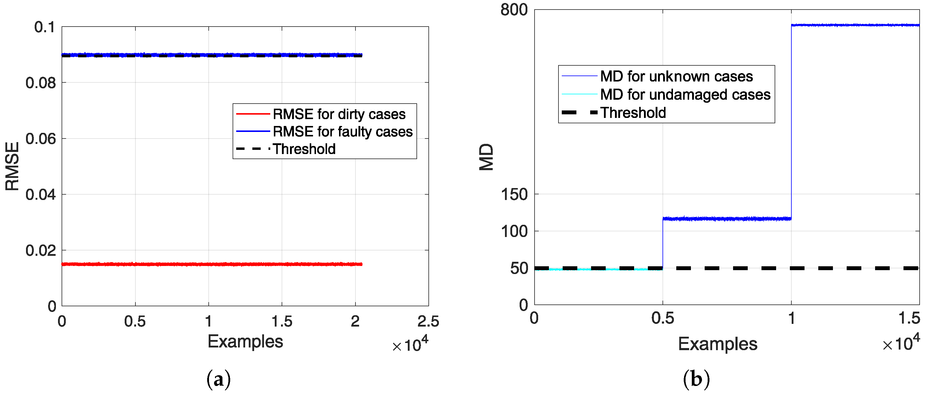
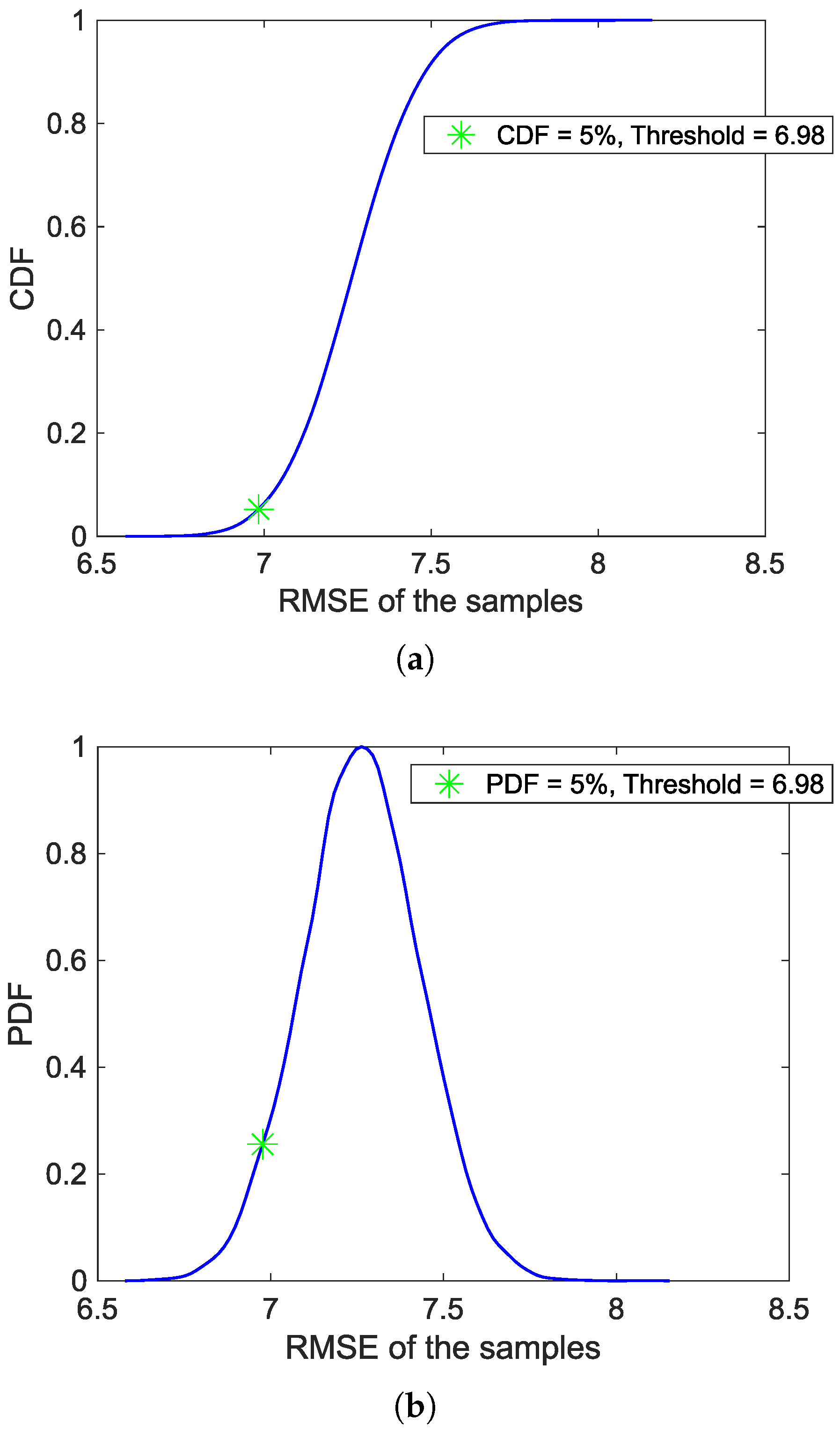
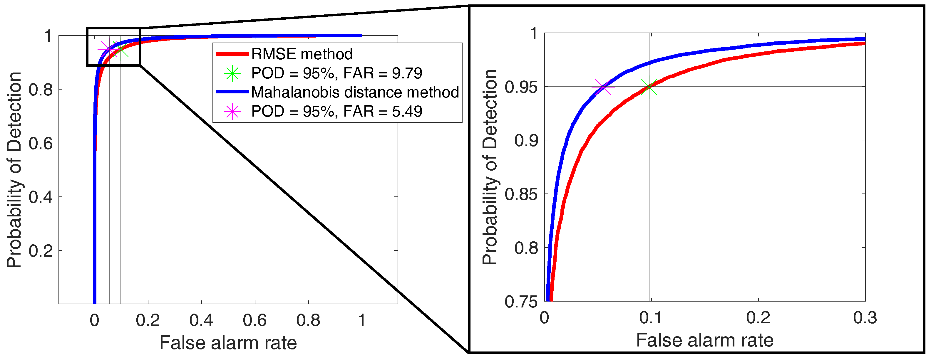
6.1. Diagnostic Algorithms’ Stress Test

To assess the robustness of diagnostic algorithms, specific cases are analysed in which the identification of the defective condition is more challenging. These scenarios involve situations requiring high accuracy, or, for example, accumulated dirt inside bearings might be mistaken for a fault when they only require cleaning operations.

6.1.1. The Steering System

Starting with the steering subsystem, the RMSEs of the faulty and healthy cases follow a Gaussian distribution due to the similarity of the signals, as visible in Figure 10. An initial threshold is estimated from the Cumulative Density Function (CDF) of the RMSEs by selecting a threshold capable of distinguishing 95% of the faulty cases, as shown in Figure 10. The choice of 95% is made considering the overlap between the RMSEs of defective and healthy cases, which is not shown to prevent reporting difficult-to-interpret results. However, the same statement can be made for the Mahalanobis distances reported in Figure 11, which is a clearer example representative of this overlap.
Since a threshold that is able to clearly distinguish between healthy and anomalous conditions cannot be selected, a threshold can be chosen by exploiting the Receiver Operating Characteristic (ROC) curve. Referring to Figure 12, which represents a generic ROC curve, that is, a plot of the probability of detection (POD) versus the false alarm rate (FAR), selecting a threshold close to 100% would include a significant portion of healthy cases, leading to a high false alarm rate. On the contrary, if one wants to reduce the false alarm rate, the probability of detection also decreases. Consequently, a threshold must be set based on a trade-off between the POD and FAR, which are defined as follows:
P O D = A l a r m | D a m a g e d D a m a g e d c a s e s
F A R = A l a r m | U n d a m a g e d U n d a m a g e d c a s e s
Thus, a threshold of 95% can be set as a trade-off between the probability of detection and the false alarm rate. As highlighted in Figure 13, the threshold that gives us a 95 % probability of detecting the damage also results in false alarm rates of 5.49 % for the Mahalanobis distance method and 9.79 % for the RMSE-based method. This highlights that the latter method performs worse than the one based on the Mahalanobis distance. In fact, to achieve the same probability of detection, the RMSE method results in a higher false alarm rate.
However, this threshold can be adjusted based on specific requirements; for example, missed detections may be considered more risky than false alarms, or vice versa. Therefore, the accuracy of the two methods can be estimated by assigning appropriate weights to false alarms and missed detections. Equation (18) defines the accuracy under the hypothesis of the same importance, i.e., weight, being ascribed to missed detections and false alarms.
a c c u r a c y = T P + T N T P + T N + F P + F N
where
  • TP is the number of successful detections.
  • TN is the number of times that healthy conditions have not been confused with damaged conditions.
  • FP is the number of false alarms.
  • FN is the number of missed detections.
Figure 14 shows the accuracy of the two methods against the POD (a) and FAR (b) for varying thresholds, and the better performance of the method based on the Mahalanobis distance is confirmed, since this method shows higher accuracy (94.70%) with respect to the method based on the RMSE (92.59%). As can be seen, the maximum accuracy is not placed in correspondence with the selected POD. However, it depends on how accuracy is defined, that is, on how the risk of a false alarm is perceived compared to the risk of a missed detection. Therefore, the accuracy can be used to quantitatively analyse the trade-off between the FAR and POD by including some weights in Equation (18) to account for the importance given to false alarms and missed detections.

6.1.2. The Retraction/Extraction System

Moving on to the retraction/extraction system, the distribution of RMSEs is Gaussian, as stated for the steering system and visible in Figure 15. This is because the RMSEs of dirty and faulty signals are close to each other, resulting in overlapping distributions. As before, the overlap between healthy and anomalous conditions is shown only for the Mahalanobis distance in Figure 16 for the same reason as in Section 6.1.1. Distinguishing between the two conditions is challenging. Therefore, a threshold is found through a trade-off between the probability of detection and the false alarm rate.
The two methods were compared according to the ROC curve, and, as in the steering system analysis, a threshold was selected by imposing a POD of 95%. Figure 17 shows the superior performance of the diagnostic method that accounts for the characteristic of the correlation between signals, that is, the Mahalanobis distance, showing an FAR of 14.32 % versus 19.45 % for the RMSE-based method. The final comparison focusses on the accuracy and is represented in Figure 18. In this case, it is clear that a slightly higher accuracy could have been achieved by lowering the selected POD. However, as stated for the steering system, it depends on how a missed detection is considered compared to a false alarm for the system under analysis.

6.1.3. The Oleo-Pneumatic Shock Absorber

Focussing on the oleo-pneumatic shock absorber, the Probability Density Function and the Cumulative Density Function of the RMSEs of the healthy and faulty pressure signals are reported in Figure 19. Similarly to the previous cases, the recognition of healthy and faulty conditions is challenging, as shown in Figure 20, since there is an overlap between these two conditions. As before, the RMSEs for this scenario are not reported, since Figure 20 is more explanatory by representing, once again, the Mahalanobis distances.
Comparing the ROC curves of the two methods, the Mahalanobis distance method demonstrated superior performance, as shown in Figure 21, showing a lower false alarm rate ( 10.91 % ) for the same probability of detection compared to the RMSE-based diagnostic algorithm ( 14.82 % ). The superior performance of the Mahalanobis distance method is confirmed by looking at Figure 22, as it has higher accuracy ( 92.05 % ) compared to the method that relies on the RMSE ( 90.79 % ).

7. Discussion

The model described in Section 3 shows a performance comparable to that of the model found in the literature that has been experimentally validated, as shown in Section 4. Furthermore, the results presented in Section 5 show that the digital twin developed for a nose landing gear is capable of representing the behaviour of the system under healthy and anomalous conditions. Thus, it is possible to use the digital twin to build a database of healthy and damaged signals that can be used to design damage detection algorithms. These algorithms can then be used within the framework of a Health and Usage Monitoring System (HUMS) to perform real-time damage detection, resulting in damage indexes capable of supporting the decision-making process. The results of the diagnostic algorithms implemented are reported in Section 6 for the three case scenarios described in Section 4.
Taking into account the results presented in Figure 7, Figure 8 and Figure 9, which are associated with the damage levels described in Section 5, it is easy to define thresholds for the damage detection algorithms described in Section 2, as both the MDs and the RMSE values for the faulty scenarios are far from the baseline values. Therefore, a stress test was required for the two algorithms to assess their performance and robustness. This was achieved by analysing scenarios for which identifying the faulty condition is more challenging. The results of the stress test are reported in Section 6.1 in terms of the Receiver Operating Characteristic (ROC) curves, that is, curves of the probability of detection against the false alarm rate, and accuracy, defined by setting equal weights to false alarms and missed detections.
Starting with the steering case study, the stress test addresses cases in which the accumulation of dirt on the bearings could be confused with damage. Looking at Figure 13, it is possible to compare the ROC curves for the two algorithms implemented. As can be seen, the Mahalanobis distance-based algorithm is the one that shows the lowest false alarm rate (6.87% against 11.98% for the RMSE-based algorithm) given the same probability of detection of 95%. Similarly, Figure 14 confirms the superior performance of the MD-based method, resulting in an accuracy of 94.70 % versus that of the RMSE-based method, that is, of 92.59 % .
Moving on to the retraction scenario, the presence of dirt on the bearings may be confused with anomalous conditions, as for the steering system. The same behaviour as in the previous case study can be observed in Figure 17 for the retraction scenario, since the Mahalanobis distance-based algorithm shows a FAR of 17.30% against 23.27% with the RMSE-based method for the same POD of 95%. In this case, the two false alarm rates are closer to each other with respect to the previous scenario, but the Mahalanobis distance method proves to be more robust than the RMSE-based one. This is reflected in the slightly lower accuracy ( 88.77 % ) of the latter method compared to the algorithm that relies on the Mahalanobis distance ( 90.33 % ).
Finally, for the third case study, that is, for the oleo-pneumatic shock absorber, small variations in the leakage area were used to perform the stress test by checking whether the algorithm could distinguish between mild and severe damages. Figure 21 shows that even in this scenario, the algorithm that relies on the Mahalanobis distance performs better relative to the algorithm that relies on the RMSE by showing an FAR of 10. 91% versus 14. 82% with the RMSE-based method. As in the previous cases, the POD is assumed to be 95%. This is reflected in the accuracies of the two methods, as the Mahalanobis distance-based algorithm results in an accuracy of 92.05 % versus 90.79 % with the other method.
Finally, it is possible to notice that the false alarm rate for the Mahalanobis distance is approximately 4–5% lower than the FAR of the RMSE-based algorithm in all scenarios implemented and for the POD value used, that is, 95 % . Similarly, the accuracy of the algorithm that relies on the Mahalanobis distance is around 2–3% higher compared to the other method. Therefore, the implementation of damage detection algorithms based on the Mahalanobis distance could be preferred by showing the lowest FAR. However, the Mahalanobis distance is based on the assumption of having a baseline that follows a Gaussian distribution. However, small deviations from normality (unimodal distributions with appropriately weighted tails) do not represent a serious concern. Otherwise, other methods must be used, such as Support Vector Machines (SVMs) or other statistical approaches that may include density estimates.
In general, the choice of the damage detection algorithm and probability of detection value should be based on an analysis considering the costs of false alarms and missed detections. The perception of the risk related to false alarms and missed detections will also be reflected in the definition of accuracy, which is defined in Equation (18) under the hypothesis that they are given the same importance, i.e., weight. Including appropriate weights in the proposed definition of accuracy can support the algorithm selection, since it is possible to quantitatively express the worst condition. For example, if a missed detection is a more serious concern than a false alarm, it is possible to quantify it in Equation (18) so that the algorithm selected can be the one that minimises missed detections. Therefore, accuracy can be effectively used as a tool to quantitatively assess the trade-off between the POD and the FAR, since its definition takes into account the perceived risk associated with false alarms and missed detections.
Focussing on computational demand, the algorithms that load the databases and perform outlier analyses run, in the worst-case scenario for computational cost, for 256.43 s. Therefore, there is no problem in running the algorithms once the aircraft has landed or, if one wants to apply them to other aircraft subsystems, almost in real time. Furthermore, the proposed framework is fully scalable in other aircraft or aircraft subsystems as long as a baseline is available for them, that is, a database of signals acquired under healthy conditions.
To conclude, it may be worth stating that the evaluation of the impact of the proposed framework on the maintenance workflow and costs is not the focus of this work. However, this approach paves the way towards maintenance optimisation because the rate of unexpected failures should decrease when continuously monitoring the aircraft, and aircraft may be stopped for maintenance only when required, preventing an aircraft in a healthy state from being stopped for planned maintenance.

8. Conclusions

In this work, a simplified model of the main subsystems of a nose landing gear has been developed using the Simulink environment. The subsystems considered are the nose wheel steering system, the retraction/extraction system, and the landing gear shock absorber, as they play crucial roles in the nose landing gear operations.
Using the Simscape libraries, it was possible to implement damages in the model, such as oil leakage in the oil chamber and a bearing fault in the steering and retraction/extraction systems, to create a database of signals in both healthy and anomalous conditions. The latter was used to implement and test damage detection algorithms, paving the way towards a condition-based maintenance approach and the design of a Health and Usage Monitoring System.
This study presents two different diagnostic algorithms to perform damage detection, which are based on the Root-Mean-Square Error and the Mahalanobis distance. The algorithm based on the Mahalanobis distance proved to be more robust than the other, with a lower false alarm rate and higher accuracy given the same probability of detection. However, the final choice of the algorithm should be based on a risk and cost analysis, taking into account the costs of having false alarms and missed detections. To support this trade-off, the proposed definition of accuracy can be adapted by adding appropriate weights to its formulation.
The framework proposed can easily be generalised since the algorithms presented are fully scalable on other aircraft and other systems more generally, as long as there is a baseline available for them, that is, a database of signals acquired under healthy conditions. The need to have a baseline arises from the fact that both algorithms express the distance of the new data with respect to a certain condition, that is, the healthy state. The farther they are from the baseline, the more probable it is that they represent an anomalous condition.
Future work shall focus on (i) improving the nose landing gear model and (ii) testing the algorithms with data from real systems. Focussing on the model, the structural flexibility of the landing gear components may be taken into account, leading to the study of the phenomena of dynamic instability, such as gear walk and shimmy. The roll, pitch, and yaw of the aircraft during landing can be considered, as they could impact the weight distribution. Considering these variables, together with the damping and cushioning effects of the tyres and the potential improvements mentioned above, would contribute to moving towards a more accurate digital twin of the nose landing gear. In addition, real-time updating of the digital twin parameters should be ensured, and part of the prognosis could be carried out, for example, by implementing damage evolution models. Moving on to the test in real scenarios, experimental campaigns may be carried out in extreme environments to observe the influence of temperature and set up algorithms to remove its effect so that anomalies will not be confounded with temperature variations. Similarly, it would be interesting to perform tests under damage conditions to build damage evolution models, allowing for the possibility of making a prognosis and therefore being able to estimate the residual useful life (RUL) of the nose landing gear.

Author Contributions

Conceptualisation, C.S. and M.G.; methodology, L.P. and O.H.; formal analysis, O.H.; writing—original draft, O.H.; writing—review and editing, L.P. and C.S.; visualisation, L.P., and C.S.; supervision, C.S.; project administration, C.S. and M.G. All authors have read and agreed to the published version of the manuscript.

Funding

This work is developed under the project ZENIT-HUMS and Vulnerability/Survivability methodologies applied to RPAS in the framework of Collaboration agreement between the Politecnico di Milano and the Italian Ministry of Defense-General Secretariat of Defense and National Armaments Directorate (ARMAEREO, II Reparto-4ª Divisione).

Data Availability Statement

Data sharing is not applicable to this article.

Acknowledgments

This work was supported by Leonardo SpA. The authors thank Renato Gollino and Josè Luis Colado Gimeno for their collaboration and support.

Conflicts of Interest

The authors declare no conflicts of interest. The funders had no role in the design of the study; in the collection, analyses, or interpretation of data; in the writing of the manuscript; or in the decision to publish the results.

References

  1. McLean, V.; Reiman, A.D. Transportation service level impact on aircraft availability. J. Def. Anal. Logist. 2022. [Google Scholar] [CrossRef]
  2. Budeanu, D.; Bylsma, G.; Cros, G.; Shannon, D.; El Helw, A.; Fernandes, K.; Goulart, A.; Hansen, M.; Harant, J.V.; Il Chan, K.; et al. Aircraft Operational Availability, 2nd ed.; Technical Report; International Air Transport Association: Montreal, QC, Canada, 2022. [Google Scholar]
  3. Brown Vows New Measures to Boost USAF Readiness. Available online: https://www.airandspaceforces.com/brown-vows-new-measures-to-boost-usaf-readiness/ (accessed on 22 November 2023).
  4. Mattis, J. Summary of the 2018 National Defense Strategy; Technical Report; U.S. Department of Defense: Washington, DC, USA, 2018.
  5. Heininen, A. Modelling and Simulation of an Aircraft Main Landing Gear Shock Absorber. Master’s Thesis, Tampereen Teknillinen Yliopisto, Tampere, Finland, 2015. [Google Scholar]
  6. Pinello, L.; Brancato, L.; Giglio, M.; Cadini, F.; De Luca, G.F. Enhancing Planetary Exploration through Digital Twins: A Tool for Virtual Prototyping and HUMS Design. Aerospace 2024, 11, 73. [Google Scholar] [CrossRef]
  7. Chiariello, A.; Orlando, S.; Vitale, P.; Linari, M.; Longobardi, R.; Di Palma, L. Development of a Morphing Landing Gear Composite Door for High Speed Compound Rotorcraft. Aerospace 2020, 7, 88. [Google Scholar] [CrossRef]
  8. Shmidt, R.K. Monitoring of Aircraft Landing Gear Structure; Royal Aeronautical Society: Hong Kong, China, 2008. [Google Scholar] [CrossRef]
  9. Forrest, C.; Forrest, C.; Wiser, D. Landing Gear Structural Health Monitoring (SHM). Procedia Struct. Integr. 2017, 5, 1153–1159. [Google Scholar] [CrossRef]
  10. Viscardi, M.; Arena, M.; Napolitano, P.; Iaccarino, P.; Cerreta, P. Complex composite technology investigation: Simulations and experimental results. In Journal of Physics: Conference Series; IOP Publishing: Bristol, UK, 2020. [Google Scholar] [CrossRef]
  11. Viscardi, M.; Arena, M.; Iaccarino, P.; Insderra Imparato, S. Manufacturing and Validation of a Novel Composite Component for Aircraft Main Landing Gear Bay. J. Mater. Eng. Perform. 2019, 28, 3292–3300. [Google Scholar] [CrossRef]
  12. Viscardi, M.; Arenza, M.; Ciminiello, M.; Guida, M.; Cerreta, P. Experimental technologies comparison for strain measurements of a composite main landing gear bay specimen. In Nondestructive Characterization and Monitoring of Advanced Materials, Aerospace, Civil Infrastructure, and Transportation XII; SPIE: Bellingham, WA, USA, 2018. [Google Scholar] [CrossRef]
  13. Mae, A.M. Cheat Sheet: What Is Digital Twin? Available online: https://www.ibm.com/blog/iot-cheat-sheet-digital-twin/ (accessed on 22 November 2023).
  14. Worden, K.; Manson, G.; Fieller, N. Damage Detection Using Outlier Analysis. J. Sound Vib. 2000, 229, 647–667. [Google Scholar] [CrossRef]
  15. Yeager, M.; Gregory, B.; Key, C.; Todd, M. On using robust Mahalanobis distance estimations for feature discrimination in a damage detection scenario. Struct. Health Monit. 2019, 18, 245–253. [Google Scholar] [CrossRef]
  16. Dervilis, N.; Cross, E.; Barthorpe, R.; Worden, K. Robust methods of inclusive outlier analysis for structural health monitoring. J. Sound Vib. 2014, 333, 5181–5195. [Google Scholar] [CrossRef]
  17. Bull, L.; Worden, K.; Fuentes, R.; Manson, G.; Cross, E.; Dervilis, N. Outlier ensembles: A robust method for damage detection and unsupervised feature extraction from high-dimensional data. J. Sound Vib. 2019, 453, 126–150. [Google Scholar] [CrossRef]
  18. Classification: ROC Curve and AUC. Available online: https://developers.google.com/machine-learning/crash-course/classification/roc-and-auc (accessed on 22 November 2023).
  19. Farrar, C.R.; Worden, K. Structural Health Monitoring: A Machine Learning Perspective; John Wiley & Sons, Ltd.: Hoboken, NJ, USA, 2013. [Google Scholar]
  20. De Maesschalck, R.; Jouan-Rimbaud, D.; Massart, D. The Mahalanobis distance. Chemom. Intell. Lab. Syst. 2000, 50, 1–8. [Google Scholar] [CrossRef]
  21. Chen, C.; Wang, Y.; Wang, T.; Yang, X. A Mahalanobis Distance Cumulant-Based Structural Damage Identification Method with IMFs and Fitting Residual of SHM Measurements. Math. Probl. Eng. 2020, 2020, 6932463. [Google Scholar] [CrossRef]
  22. Daga, A.P.; Fasana, A.; Marchesiello, S.; Garibaldi, L. The Politecnico di Torino rolling bearing test rig: Description and analysis of open access data. Mech. Syst. Signal Process. 2019, 120, 252–273. [Google Scholar] [CrossRef]
  23. Figueiredo, E.; Park, G.; Farrar, C.R.; Worden, K.; Figueiras, J. Machine learning algorithms for damage detection under operational and environmental variability. Struct. Health Monit. 2011, 10, 559–572. [Google Scholar] [CrossRef]
  24. Gul, M.; Necati Catbas, F. Statistical pattern recognition for Structural Health Monitoring using time series modeling: Theory and experimental verifications. Mech. Syst. Signal Process. 2009, 23, 2192–2204. [Google Scholar] [CrossRef]
  25. Figueiredo, E.; Radu, L.; Worden, K.; Farrar, C.R. A Bayesian approach based on a Markov-chain Monte Carlo method for damage detection under unknown sources of variability. Eng. Struct. 2014, 80, 1–10. [Google Scholar] [CrossRef]
  26. Bao, C.; Hao, H.; Li, Z. Vibration-based structural health monitoring of offshore pipelines: Numerical and experimental study. Struct. Control Health Monit. 2013, 20, 769–788. [Google Scholar] [CrossRef]
  27. Entezami, A.; Shariatmadar, H.; Mariani, S. Early damage assessment in large-scale structures by innovative statistical pattern recognition methods based on time series modeling and novelty detection. Adv. Eng. Softw. 2020, 150, 102923. [Google Scholar] [CrossRef]
  28. Manring, N.D.; Fales, R.C. Hydraulic Control Systems; John Wiley & Sons, Inc.: Hoboken, NJ, USA, 2005. [Google Scholar]
  29. Universal and Individual Gas Constants. Available online: https://www.engineeringtoolbox.com/individual-universal-gas-constant-d_588.html (accessed on 22 November 2023).
  30. Hydraulic Fluid. Available online: https://it.mathworks.com/help/hydro/ref/hydraulicfluid.html (accessed on 22 November 2023).
  31. Heininen, A.; Aaltonen, J.; Koskinen, K.; Huitula, J. Equations of State in Fighter Aircraft Oleo-Pneumatic Shock Absorber Modelling; Tampere University: Tampere, Finland, 2019; pp. 64–70. [Google Scholar] [CrossRef]
  32. Dixon, J.C. The Shock Absorber Handbook, 2nd ed.; John Wiley and Sons, Ltd.: Hoboken, NJ, USA, 2007. [Google Scholar]
  33. Armstrong, B.; de Wit, C. Friction Modeling and Compensation, The Control Handbook; CRC Press: Boca Raton, FL, USA, 1995. [Google Scholar]
  34. Li, K. Developing More Electric Aircraft Technologies. Int. Aviat. 2009, 1, 73–75. [Google Scholar]
  35. Mathworks. Motor & Drive (System Level)-Simscape Library Documentation. 2023. Available online: https://uk.mathworks.com/help/sps/ref/motordrivesystemlevel.html (accessed on 22 November 2023).
  36. Skorupka, Z.; Kowalski, W.; Kajka, R. Electrically Driven and Controlled Landing Gear for UAV up to 100 kg of Take off Mass. In Proceedings of the 24th European Conference on Modelling and Simulation, Kuala Lumpur, Malaysia, 1–4 June 2010; pp. 1–5. [Google Scholar]
  37. Components of an Electric Linear Actuator. Available online: https://www.progressiveautomations.com/blogs/products/inside-an-electric-linear-actuator (accessed on 22 November 2023).
  38. Shams, T.A.; Shah, S.I.A.; Ahmad, M.A.; Mehmood, K.; Ahmad, W.; Rizvi, S.T.u.I. Selection Methodology of an Electric Actuator for Nose Landing Gear of a Light Weight Aircraft. Appl. Sci. 2020, 10, 8730. [Google Scholar] [CrossRef]
  39. Na, K.m.; Hwang, K.L. Airworthiness Certification of Unmanned Aerial System; Technical Report; Defense Acquisition Program Administration-European Defense Agency: Brussels, Belgium, 2017; Available online: https://eda.europa.eu/docs/default-source/events/mac2017/3-7_certification-of-unmanned-aerial-system—rok.pdf (accessed on 22 November 2023).
  40. Van Damme, J.; Vansompel, H.; Crevecoeur, G. Stall Torque Performance Analysis of a YASA Axial Flux Permanent Magnet Synchronous Machine. Machines 2023, 11, 487. [Google Scholar] [CrossRef]
  41. Kerr, T.; Barrett, S. Motor Control and Actuators. In Arduino IV: DIY Robots: 3D Printing, Instrumentation, and Control; Springer International Publishing: Cham, Switzerland, 2022; pp. 161–188. [Google Scholar] [CrossRef]
  42. Fracasso, D. Digital-Twin for Health Monitoring of an Aircraft’s Elevon; Milan Institute of Technology: Milan, Italy, 2022. [Google Scholar]
  43. Miller, S. Predictive Maintenance in a Hydraulic Pump. 2023. Available online: https://www.mathworks.com/matlabcentral/fileexchange/65605-predictive-maintenance-in-a-hydraulic-pump (accessed on 22 November 2023).
Figure 1. A schematic of the oleo-pneumatic shock absorber. The nitrogen chamber is represented in blue, while the oil chamber consists of a primary part, in yellow, and a secondary part, in purple.
Aerospace 11 00222 g001
Figure 2. A comparison of the sinking velocity with a reference from the literature. (a) The compression velocity in [5]. (b) The compression velocity during the aircraft landing simulation.
Aerospace 11 00222 g002
Figure 3. A comparison of the shock absorber stroke with the literature reference. (a) The normalised stroke in [5]. (b) The stroke of the shock absorber during the aircraft landing simulation.
Aerospace 11 00222 g003
Figure 4. The rotation of the steering actuator for different conditions of the linkage bearing.
Aerospace 11 00222 g004
Figure 5. The normalised stroke of the linear actuator for different conditions of the trunnion bearing.
Aerospace 11 00222 g005
Figure 6. The normalised stroke of the shock absorber for different oil leakage levels.
Aerospace 11 00222 g006
Figure 7. Mahalanobis distances and RMSEs for right-turn simulations. (a) RMSEs for steering simulations. (b) Mahalanobis distances for right-turn simulations.
Aerospace 11 00222 g007
Figure 8. Mahalanobis distances and RMSEs for retraction simulations. (a) RMSEs for retraction simulations. (b) Mahalanobis distances for retraction simulations.
Aerospace 11 00222 g008
Figure 9. Mahalanobis distances and RMSEs for aircraft landing simulations. (a) RMSEs for aircraft landing simulations. (b) Mahalanobis distances for landing simulations of aircraft.
Aerospace 11 00222 g009
Figure 10. The Probability Density Function (PDF) and Cumulative Density Function (CDF) of the RMSEs for dirty and faulty steering simulations. (a) The CDF of the RMSEs of the steering simulations. (b) The PDF of the RMSEs of the steering simulations.
Aerospace 11 00222 g010
Figure 11. Mahalanobis distances for dirty and faulty steering simulations.
Aerospace 11 00222 g011
Figure 12. Receiver Operating Characteristic (ROC) curve: probability of detection vs. false alarm rate.
Aerospace 11 00222 g012
Figure 13. POD vs. FAR for the two implemented methods in the steering simulations.
Aerospace 11 00222 g013
Figure 14. Plots of accuracy against the POD and the FAR for the two methods implemented for the steering simulations. (a) A plot of accuracy against the POD for the steering simulations. (b) A plot of accuracy against the FAR for the steering simulations.
Aerospace 11 00222 g014
Figure 15. The Probability Density Function (PDF) and Cumulative Density Function (CDF) of the RMSEs for dirty and faulty retraction simulations. (a) The CDF of the RMSEs of the retraction simulations. (b) The PDF of the RMSEs of the retraction simulations.
Aerospace 11 00222 g015
Figure 16. Mahalanobis distances for dirty and faulty retraction simulations.
Aerospace 11 00222 g016
Figure 17. POD vs. FAR for the two implemented methods in the retraction simulations.
Aerospace 11 00222 g017
Figure 18. Plots of the accuracy against the POD and the FAR for the two methods implemented for the retraction simulations. (a) The plot of accuracy against the POD for the retraction simulations. (b) A plot of accuracy against the FAR for the retraction simulations.
Aerospace 11 00222 g018aAerospace 11 00222 g018b
Figure 19. The Probability Density Function (PDF) and Cumulative Density Function (CDF) of the RMSEs for lightly and severely faulted aircraft landing simulations. (a) The CDF of the RMSEs of the landing simulations. (b) The PDF of the RMSEs of the landing simulations.
Aerospace 11 00222 g019aAerospace 11 00222 g019b
Figure 20. Mahalanobis distances for dirty and faulty landing simulations.
Aerospace 11 00222 g020
Figure 21. POD vs. FAR for the two implemented methods in the landing simulations.
Aerospace 11 00222 g021
Figure 22. Plots of the accuracy against the POD and the FAR for the two methods implemented for the landing simulations. (a) The plot of accuracy against the POD for the landing simulations. (b) The plot of accuracy against the FAR for the landing simulations.
Aerospace 11 00222 g022
Table 1. Safety factors in the nose landing gear steering scenario.
TorqueAngular Velocity
η = M a x i m u m A d m i s s i b l e V a l u e M a x i m u m S i m u l a t i o n V a l u e 3.91.1
Table 2. Safety factors in the nose landing gear retraction scenario.
ForceActuator Stroke
η = M a x i m u m A d m i s s i b l e V a l u e M a x i m u m S i m u l a t i o n V a l u e 2.31.03
Table 3. Safety factors in the landing scenario.
Sinking VelocityShock Absorber Stroke
η = M a x i m u m A d m i s s i b l e V a l u e M a x i m u m S i m u l a t i o n V a l u e 1.962.3
Disclaimer/Publisher’s Note: The statements, opinions and data contained in all publications are solely those of the individual author(s) and contributor(s) and not of MDPI and/or the editor(s). MDPI and/or the editor(s) disclaim responsibility for any injury to people or property resulting from any ideas, methods, instructions or products referred to in the content.

