Characterizing Satellite Geometry via Accelerated 3D Gaussian Splatting

Abstract

The accelerating deployment of spacecraft in orbit has generated interest in on-orbit servicing (OOS), inspection of spacecraft, and active debris removal (ADR). Such missions require precise rendezvous and proximity operations in the vicinity of non-cooperative, possibly unknown, resident space objects. Safety concerns with manned missions and lag times with ground-based control necessitate complete autonomy. This requires robust characterization of the target’s geometry. In this article, we present an approach for mapping geometries of satellites on orbit based on 3D Gaussian splatting that can run on computing resources available on current spaceflight hardware. We demonstrate model training and 3D rendering performance on a hardware-in-the-loop satellite mock-up under several realistic lighting and motion conditions. Our model is shown to be capable of training on-board and rendering higher quality novel views of an unknown satellite nearly 2 orders of magnitude faster than previous NeRF-based algorithms. Such on-board capabilities are critical to enable downstream machine intelligence tasks necessary for autonomous guidance, navigation, and control tasks.

1. Introduction

The recent reduction in the costs of launching spacecraft has led to an acceleration in the deployment of large satellite constellations and human spaceflight exploration missions. However, retired satellites and collisions of space objects in orbit have resulted in an exponential rise in untracked space debris. This poses collision risks to new launches, which could spread thousands of new pieces of debris, causing catastrophic cascading failures.

Numerous efforts in the field of robotic active debris removal (ADR) and on-orbit servicing (OOS) have been conducted around known cooperative and non-cooperative spacecraft. In 1997, ETS-VII [1] by NASDA (now JAXA) made a groundbreaking leap by demonstrating the first-ever autonomous docking procedure with a target (cooperative) spacecraft. Following that, other technology development missions were conducted around cooperative spacecraft, such as NASA, DARPA, AFRL’s DART, XSS-10 [2], XSS-11 [3], ANGELS [4], MiTEX, and Orbital Express. In 2020 and 2021, Northrup Grumman conducted the first-ever commercial OOS operations with its MEV-1 [5] and MEV-2 [6,7] satellites to take over the stationkeeping of IS-901 and IS-10-02, respectively. In 2022, as part of a demonstration of the autonomous capture of an uncontrolled object, Astroscale’s ELSA-d mission’s servicer demonstrated the ability to autonomously rendezvous with the client prior to pausing the mission due to failed thrusters [8]. All these missions were conducted around known and/or cooperative target objects. However, in reality, resident space objects (RSOs) may have unknown structures, masses, geometries, and attitudes. Performing OOS around unknown, non-cooperative spacecraft remains an unresolved challenge.

To perform OOS and ADR around these unknown RSOs, it is essential to autonomously characterize their geometries, identify points for capture, plan and execute safe approach paths, capture the target, and stabilize its attitude. Distributed satellite systems (DSS), groups of small, cooperative satellites, each equipped with a system for relative navigation, a robust propulsion system, and a flexible capture mechanism, offer a scalable solution for OOS and ADR tasks involving large non-cooperative targets as DSS swarms can distribute the forces and moments required to detumble an RSO. A concept of a DSS is illustrated in Figure 1.

Working together, these satellite swarms characterize the target’s geometry (the focus of this article), assess its motion and structural condition, pinpoint possible capture points and collision risks, devise safe approach routes to these points, and collectively plan and carry out maneuvers to stabilize the target’s spin. The complexity of these operations, especially the skills needed for mapping the geometry accurately, necessitates the application of machine learning technologies. This is crucial to replicate the inherent abilities of humans in these tasks.

The complexity of this approach necessitates complete autonomy during the rendezvous and proximity operation (RPO) phases. Although previous research has shown the integration of AI-based machine vision for navigation [10] and artificial potential field for guidance [11,12] as a feasible method for autonomous rendezvous with these unknown RSOs, this approach required multiple observers along with multiple chasers in the system. Although theoretically feasible, it is impractical for real-world application, leading to a need for more streamlined and effective solutions in autonomous space servicing missions.

It is much preferred to deploy a single observer that will inspect and fully characterize the geometry and components of the non-cooperative RSO, then guide the chasers, but this requires the full characterization of the geometry and components (e.g., satellites and antennas) of the RSO using on-board spaceflight hardware. While multi-observer swarms can characterize an RSO’s 3D geometry by triangulating points several observers can view, this is more challenging for a single observer.

This article aims to tackle the first of these two problems: characterizing the geometry of an RSO at low computational cost. This is key in developing software to enable autonomous RPO with a single observer. 3D Gaussian splatting [13] is deployed to characterize the geometry of a target RSO and generate novel viewing angles of it to build a full 3D understanding of the RSO.

The primary contributions of this article include:

• An effective low-computational-cost 3D Gaussian splatting model optimized for the 3D reconstruction of an unknownRSO capable of deployment on spaceflight hardware;
• Hardware-in-the-loop experiments demonstrating 3D rendering performance under realistic lighting and motion conditions;
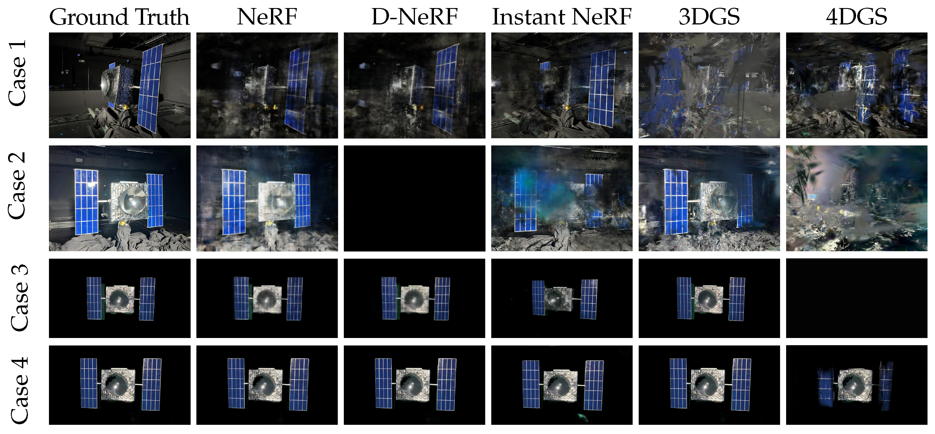
• A comparison of the NeRF, D-NeRF, Instant NeRF, 3D Gaussian splatting, and 4D Gaussian splatting algorithms in terms of 3D rendering quality, runtimes, and computational costs.

2. Related Work

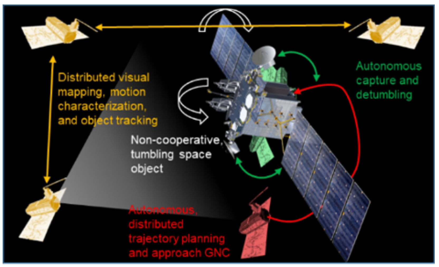
2.1. Computer Vision for On-Orbit Operations

Traditional computer vision techniques are widely familiar in the field of guidance, navigation, and controls and act as the first step to navigation. However, traditional techniques are limited to the presence of known/cooperative features, which is not the case for unknown satellites. In recent years, neural network-based computer vision techniques have shown highly promising results for performing in non-cooperative environments and are actively being used for autonomous navigation in robotics and the automobile industry, for example. Extensive research is being performed to identify and track [14] components of non-cooperative known spacecraft [15] and unknown spacecraft [10,16,17,18], such as solar panels, antennas, bodies, and thrusters. Knowing the presence of the components and their relative positions could assist with autonomously rendezvousing to an RSO, as shown in [12,19]. However, as described earlier, being able to characterize an RSO with a single observer reduces the risk of collision while improving reliability in the navigation model.

Research derived from the spacecraft pose estimation challenge based on datasets [20,21] show that the pose of a known non-cooperative spacecraft can be reliably estimated using a monocular camera [22,23,24,25]. However, these techniques fail for an unknown spacecraft.

Photogrammetry techniques based on neural radiance fields (NeRFs) [26] and generative radiance fields (GRAFs) [27] have gained significant popularity in performing the 3D reconstruction of an object based on images. In [28], NeRF and GRAF generated 3D models of SMOS and a CubeSat, with the results showing that NeRF achieved better performance than GRAF. In [29], the authors further investigated NeRF along with instant NeRF [30] and dynamic NeRF [31] on hardware-in-the-loop (HIL) images of a satellite mockup. It was concluded that instant NeRF, which is capable of running on hardware with spaceflight heritage [32], is preferred for its fast computational time and relatively good performance. In [33], the author took a unique approach to identifying the pose of an unknown spacecraft by fitting superquadrics in the mask of a single satellite image. Though this approach effectively identified high-level details, such as solar panels, it lacked smaller crucial details, such as apogee kick motors (if present) or smaller cylindrical rods, as well as the ability to check if a component that may be a potential docking feature is still intact, as described in [12].

2.2. 3D Rendering

Characterizing the 3D geometry of an unknown RSO with a single data feed is a challenging task. Until recently, there were few prospects to perform this task with high visual quality. However, recent work in the computer vision community, as discussed below, has made this more feasible.

Neural radiance fields (NeRFs) [26] use a fully connected neural network to learn a radiance field that can render synthetic views of 3D scenes. NeRFs map spatial locations and viewing angles represented as 5D coordinates $(x,y,z,\theta ,\varphi )$ to opacity and view-dependent colors at all locations in space. The neural network estimates the opacities and colors, and rays are traced through them to compute the pixel colors of an observer’s 2D viewframe of a 3D scene, an approach called volumetric rendering.

The NeRF process is differentiable end-to-end, so these models can be trained with standard gradient-based methods. NeRF is effective at generating high-quality views of 3D scenes but has slow training and rendering times. It also only considers static scenes, which limits the possibility of movement in the scene.

Accelerating NeRF. Instant NeRF [30] accelerates NeRF training. It learns a multi-resolution set of feature vectors called neural graphics primitives that encode input scenes more efficiently. This enables Instant NeRF to produce similar results for NeRF with a much smaller neural network that trains with a far smaller computational footprint, but the rendering costs are similar to NeRF.

3D Gaussian splatting [13] is a recent method that learns a Gaussian point-based representation of a 3D scene slightly faster than instant NeRF but renders 1080p ($1920\times 1080$ resolution) 2D views of the scene at just 5% of the computational cost. This method uses images of the 3D scene calibrated by Structure-from-Motion (SfM) [34]. SfM computes sparse cloud of points identified in 3D based on multiple images, where 3D Gaussian random variables are initialized before being trained to represent the 3D scene. Replacing a NeRF representation with a point-based representation reduces the training time since there is no huge neural network to optimize. In addition, the point-based scene representation avoids NeRF’s reliance on a full volumetric representation of the scene. Hence, 3D splatting avoids NeRF’s expensive sampling of points on the paths traced by each ray and passing them through a large neural network.

The 3D Gaussian representation instead uses “splats”, or layers of simple textures (“image primitives”), which are mixed by the Gaussian densities at different locations in space. Novel views are rendered using separate tiles of the whole screen. GPU-accelerated sorting algorithms allow extremely fast mixing to generate tiles by only considering the splats that will be visible.

Dynamic scenes. Dynamic NeRF (D-NeRF) [31] reconstructs and renders novel images of objects from rigid and non-rigid motions from a single camera moving around the scene. It considers time as an additional input and splits the learning process of the fully connected network into two parts: one encodes the scene into a canonical space, and one maps this canonical representation into the deformed scene at a particular time. The canonical network is trained to take in 3D coordinates and the viewing directions to yield a radiance field. Then, the deformation network outputs the displacement that takes the point to its position in the canonical space. D-NeRF can render dynamic scenes and retains high-quality image details. While D-NeRF performs better with dynamic scenes, it still faces slow training and rendering difficulties.

4D Gaussian splatting [35] proposes a representation that uses the 3D Gaussian splatting point-based representation and 4D neural voxels. Similar to D-NeRF, the framework is split into a 3D scene representation and a deformation field. However, the two pieces are time-dependent 3D Gaussian representations that can be rendered using a differential splatting process. 4D Gaussian splatting is reported to produce high-quality dynamic scenes with faster training and rendering times than D-NeRF.

3. Methods

This section discusses the implementations of 3D rendering, as well as the experimental setup, datasets, and performance metrics, used in this work.

3.1. 3D Gaussian Splatting

3D Gaussian splatting has three parts: (1) structure-from-motion (SfM) learns using 2D ground-truth images to calibrate the camera views of a 3D scene by learning a common point cloud representation; (2) the SfM point cloud is repurposed to initialize a 3D Gaussian point-based representation of the 3D scene; and (3) splatting techniques are used to render novel 2D views of the scene. We discuss these three steps in details below.

Camera calibration with SfM. SfM reconstructs the 3D structure of the target. This involves estimating camera parameters and creating a three-dimensional point cloud for the target. We used COLMAP [34] to perform the spare reconstruction of the data images. COLMAP first performs feature detection and extraction on the presented images; then, it extracts points of interest and certain features from the images that will be used in the SfM algorithm. Then, a geometric verification was performed to ensure that the images that see the same scene are overlapping. Since the first matching portion did this visually, it was necessary to mathematically verify that the matched features mapped to the same point in the scene. We implemented COLMAP with the standard pinhole camera model.

COLMAP cycles through the data given and estimates camera parameters and poses for the images. The triangulation process can extend the set of scene points, which increases coverage. A new point can be triangulated once there is another image of the scene from a different viewing angle. This can provide more correspondences between the 2D images and 3D reconstruction and produces a point cloud as a byproduct.

3D Gaussian point-based representation. 3D Gaussisan splatting repurposes the SfM point cloud to initialize the means of a set of 3D Gaussian random variables. Each Gaussian random variable can be defined by its mean $p\in {\mathbb{R}}^3$ and covariance matrix $\mathsf{\Sigma }\in {\mathbb{R}}^{3\times 3}$, with a probability density of

$$\begin{array}{c}\hfill f\left(x\right)=\frac{1}{{\left(2\pi \right)}^{\frac{3}{2}}\sqrt{\left|\mathsf{\Sigma }\right|}}{e}^{-\frac{1}{2}{(x-p)}^T{\mathsf{\Sigma }}^{-1}(x-p)}\end{array}$$

(1)

at a given point $x\in \mathbb{R}$.

The means are initialized to the positions of the SfM points, and the covariances are initialized to isotropic covariances (diagonal matrices) based on the 3 nearest SfM point neighbors. In addition, each Gaussian is equipped with a multiplier $\alpha \in [0,1]$ representing the opacity for capturing radiated light and spherical harmonics coefficients representing the viewing angle-dependent color of each Gaussian. This set of Gaussians with their means, covariances, opacities, and spherical harmonic coefficients are optimized to learn a full representation of the 3D scene using only a discrete set of points.

3D Gaussian splatting-based rendering. Splatting uses graphics primitives (e.g., textures) that extend outward from individual points to ellipsoids. The 3D Gaussian densities within these ellipsoids allow Gaussian mixing with the $\alpha$ opacities (known as $\alpha$-blending in the computer graphics community). Then, 2D views can be generated with these more complex image primitives rather than simply color and opacity in NeRF’s full volumetric rendering.

The spatial extent of the splats allows point-based rendering to render equivalent- or higher-quality filled-in geometry without volumetric ray tracing. 3D Gaussian splatting uses a tile-based rasterizer that pre-sorts the Gaussian splats using a GPU radix search for the entire image. This allows fast tile-based $\alpha$-blending without per-pixel rendering of points. This procedure generates the required 2D views.

Optimizing the 3D representation. After SfM, the entire 3D Gaussian Splatting process, both training the representation and 3D rendering, is differentiable end-to-end. This enables backpropagation and gradient-based optimization. The sparse point-based rendering faces some additional challenges in terms of how many points to use, so the method additionally has a stage where it creates or destroys Gaussians during the optimization process of the Gaussian means, covariances, and associated opacities and spherical harmonic coefficients. The Gaussian covariance matrices cannot be treated as unconstrained parameters, as this would violate the definition of covariance, and hence, the technique constrains the covariances to ensure the level sets of the probability densities shown in (1) remain ellipsoids.

The loss function used for optimizing the scene representation and renders is as follows:

$$\begin{array}{c}\hfill (1-\lambda ){\mathcal{L}}_1+\lambda {\mathcal{L}}_{\text{D-SSIM}}.\end{array}$$

(2)

Minimizing the first term minimizes the pixel difference between between 2D renders and ground-truth images from the same viewing positions and angles. Minimizing the second term aims to increase SSIM between the images. We adopt the authors’ use of $\lambda =0.2$.

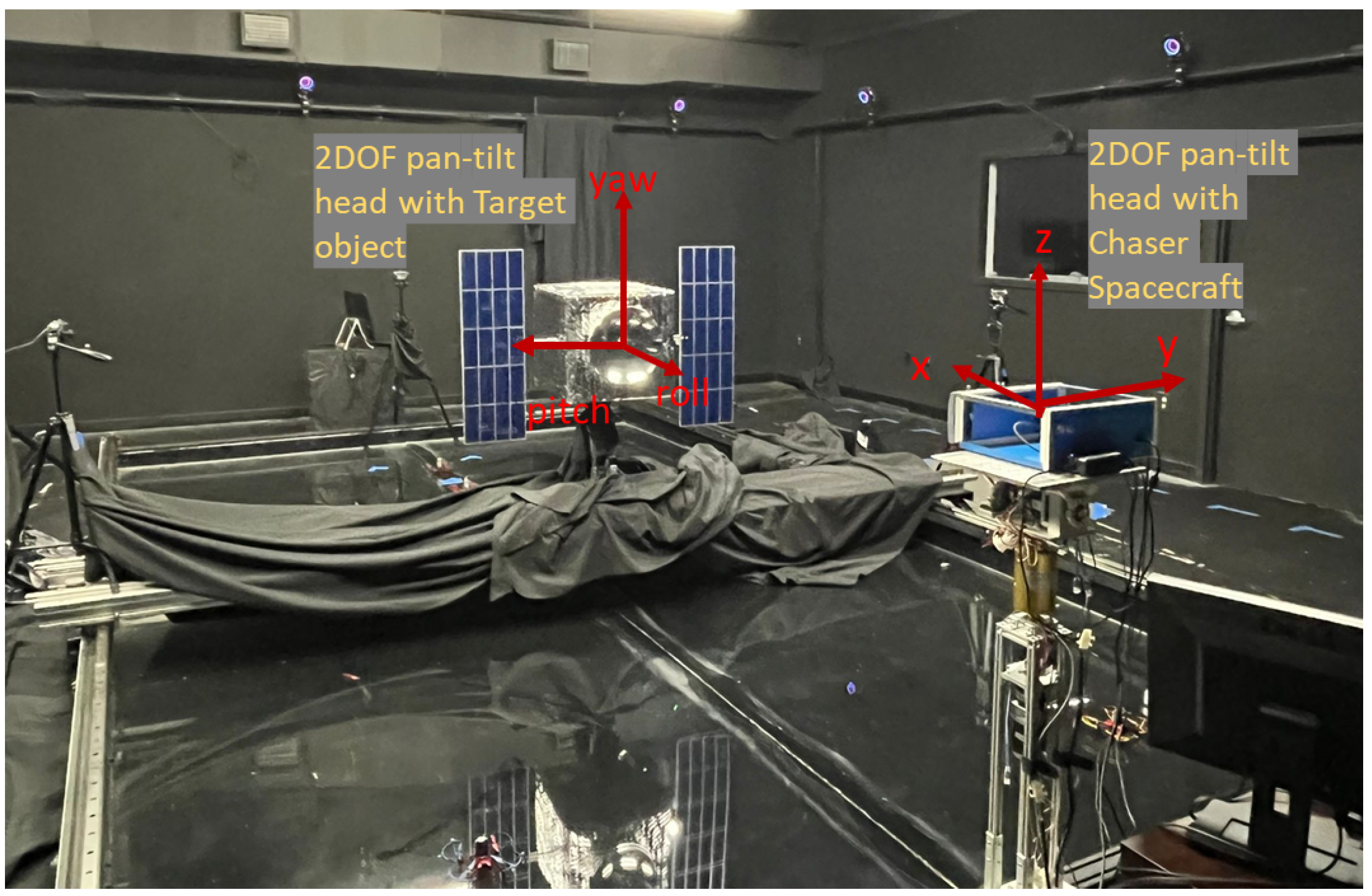
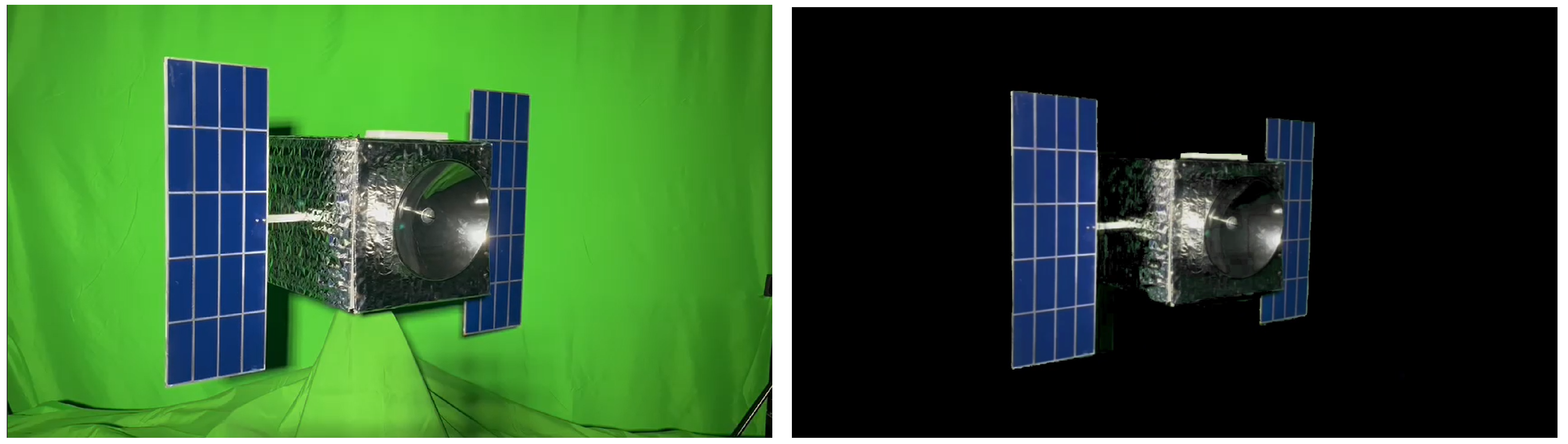
3.2. Experimental Setup

HIL data were captured on the ORION testbed [36] in the Autonomy Lab at Florida Tech. The test bed consisted of a planar, Cartesian maneuver kinematics simulator, shown in Figure 2, with a workspace of 5.5 m × 3.5 m. The simulator was equipped with a 2 DOF motion table that can translate at a maximum speed of 0.25 m/s with a maximum acceleration of 1 m/s². The simulator was equipped with two custom-designed pan-tilt mechanisms, both of which were capable of rotating infinitely in the azimuth direction (yawing) and can rotate in elevation by $\pm {90}^{\circ }$. In addition, one of the pan-tilt mechanisms (target object) can translate in the x and y axes. The target and the chaser spacecraft can be interchanged as needed. The target mock-up satellite used for this work has typical components found on a satellite, such as rectangular solar arrays, a distinct body, thruster nozzles, and a parabolic antenna.

To limit external lighting conditions, the doors, walls, and floor of the testbed were painted with low-reflectivity black paint, and the windows were closed and covered with black-out blinds, as well as black-out stage curtains. The lighting conditions for the experiments were simulated by a Hilio D12 LED panel with a color temperature of 5600 K (daylight-balanced) rated for 350 W of power with adjustable intensity. The maximum intensity of the panel was equivalent to a 2000 W incandescent lamp. The intensity of the lamp was set to 10% or 100% in the scenarios described in the next section.

3.3. Datasets

Four HIL datasets [29] were captured for training and evaluating the 3D rendering models. In all cases, images were captured using an iPhone 13 from viewing angles 360° around the satellite with the lamp pointing directly at the mock-up. To avoid including OptiTrack markers in the dataset images, viewing angles relative to the target mock-up were initially marked on the testbed floor using a compass map and verified by OptiTrack. The camera aperture was positioned at a height of 3 feet 8 inches from the ground on these marked positions as applicable. Each image and video was scaled to a resolution of 640 by 480.

The four cases differed in terms of the lighting, motion conditions, and backdrop of the images. They were captured as follows:

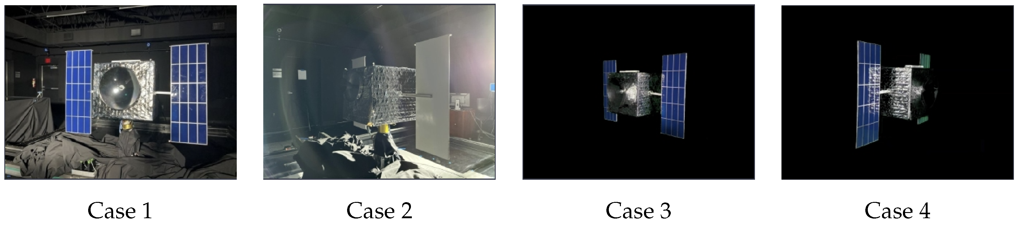
Case 1.

Images of the target RSO were taken at 10° increments around a circle with a radius of 5 ft (simulating an R-bar maneuver around a stationary RSO) with 10% lighting intensity. Viewing angles were at 10° increments rotating about the vertical axis.

Case 2.

Images of the target RSO were taken at 10° increments around a circle with a radius of 5 ft (simulating an R-bar maneuver around a stationary RSO) with 100% lighting intensity. Viewing angles were at 10° increments rotating about the vertical axis.

Case 3.

Videos of the RSO were captured as it yawed at 10°/s with the chaser positioned 5 ft away (simulating V-bar stationkeeping around a spinning RSO) with 10% lighting intensity. Viewing angles were at 5° increments rotating about the vertical axis.

Case 4.

Videos of the RSO were captured as it yawed at 10°/s with the chaser positioned 5 ft away (simulating V-bar stationkeeping around a spinning RSO) with 100% lighting intensity. Viewing angles were at 5° increments rotating about the vertical axis.

In Cases 3–4, we placed a green screen behind the satellite mock-up. Using chroma key compositing, we then post-processed the images by replacing all green pixels with black. The results before and after pre-processing can be seen in Figure 3.

We display images from each of the four cases in Figure 4.

3.4. Performance Evaluation for 3D Rendering

We measured the performance of the 3D rendering models trained herein in terms of both their rending quality and computational requirements. In this subsection, we describe the metrics used.

The quality of the renders generated by of each model trained in this work was evaluated by qualitative comparisons of individual renders, as well as standard metrics for generative modeling, including the structural similarity index (SSIM) [37], peak signal-to-noise ratio (PSNR), and learned perceptual image patch similarity (LPIPS) [38], which were evaluated on images of the satellite mock-up not used during training.

The SSIM measures the difference between the original picture and the reconstructed image and accounts for changes such as luminance or contrast. High SSIM values indicate high performance. The PSNR measures the quality of rendered images at the pixel level. A high PSNR indicates good performance. The LPIPS is a more advanced metric that aims to capture the human-perceived similarity between images. It feeds both a real and a synthetic image patch to a VGG network [39] trained to classify the ImageNet dataset [40], extracts the hidden representations of each patch within different layers of VGG, and computes the distance between them. This distance is fed to a model to mimic human preferences, yielding the LPIPS score. Lower LPIPS scores indicate that the synthetic images are more similar to real images.

In addition, both methods were evaluated in terms of their computational requirements during both training and inference (i.e., 3D rendering). For training, we compared VRAM usage and training time. For inference (i.e., rendering), we compared VRAM usage and framerate (frames per second—FPS). VRAM usage was measured with the nvidia-smi pmon monitoring utility every 1 s, using the highest number logged, when all data and the current model were fully loaded in the GPU. For the FPS measurement process, it is important to note that, due to the extra time taken for the data and model to be copied from the CPU to the GPU, the first couple rendering runs were slower until the data were fully cached. Hence, we measured FPS by looping the render task on the test set for 10–20 iterations; we then took the average of the median 5 runs.

4. Results

In this section, we present the 3D rendering results and performance of 3D Gaussian splatting (3DGS) on all test datasets and compare them with several competing methods, including NeRF [26], D-NeRF [31], Instant NeRF [30], and 4D Gaussian splatting (4DGS) [35]. The new results differ from our previous work [29] because they limit the quantitative analysis to images in the training set, while novel renders were analyzed qualitatively.

At a first glance, a trend discussed in Caruso et al. [29] reappeared regardless of the differences in methodology: dynamic scene (D-NeRF, 4DGS) reconstruction methods consistently performed worse (

Table 1. Quality of 3D renders by models and different test cases. For each metric, ↑ indicates higher values are better and ↓ indicates lower values are better. Bolded values are the best across all methods.

Method	Case 1			Case 2			Case 3			Case 4
	SSIM↑	PSNR↑	LPIPS↓	SSIM↑	PSNR↑	LPIPS↓	SSIM↑	PSNR↑	LPIPS↓	SSIM↑	PSNR↑	LPIPS↓
NeRF	0.3891	16.81	0.5503	0.4520	16.52	0.5008	0.9332	28.24	0.0763	0.6438	19.54	0.3207
D-NeRF	0.3783	16.76	0.5418	0.0337	9.22	0.5877	0.8156	16.66	0.1853	0.6184	19.61	0.3282
Instant NeRF	0.5149	16.47	0.4374	0.4729	14.71	0.4440	0.8571	17.55	0.1277	0.8569	19.99	0.1056
3DGS	0.9223	25.70	0.0814	0.6803	16.78	0.2949	0.8756	26.53	0.1040	0.9213	25.52	0.0796
4DGS	0.5192	16.78	0.4310	0.4877	13.17	0.5193	0.4358	15.07	0.1454	0.7619	17.16	0.1890

) and took longer to train (

Table 2. Computational requirements for model training. C/T is the ratio of CUDA cores to training time (in seconds). For each metric, ↑ indicates higher values are better and ↓ indicates lower values are better. Bolded values are the best across all methods.

Method	Case 1		Case 2		Case 3		Case 4		Average
	VRAM (MB)↓	Training Time↓	VRAM (MB)↓	Training Time↓	VRAM (MB)↓	Training Time↓	VRAM (MB)↓	Training Time↓	VRAM (MB)↓	Training Time↓	C/T↑
NeRF	3833	54 m 24 s	3845	55 m 47 s	4195	1 h 18 m 21 s	3952	1 h 15 m 24 s	3956.25	1 h 5 m 59 s	2.58
D-NeRF	4586	1 h 37 m 17 s	4598	1 h 39 m 32 s	4948	2 h 14 m 56 s	4634	2 h 05 m 24 s	4691.5	1 h 54 m 17 s	1.49
Instant NeRF	1664	5 m 18 s	1684	5 m 7 s	1934	6 m 11 s	1702	6 m 15 s	1746	5 m 43 s	29.85
3DGS	1485	5 m 42 s	1668	7 m 4 s	1875	6 m 59 s	1792	6 m 32 s	1705	6 m 34 s	25.99
4DGS	2224	57 m 32 s	4089	1 h 5 m 51 s	5385	44 m 34 s	5022	1 h 56 m 00 s	4180	1 h 10 m 59 s	2.40

) than their static counterparts (NeRF, Instant NeRF, 3DGS). In addition, training VRAM usage metrics shows these dynamic scene models also consume more resources. As such, our previous conclusion still stands: static scene reconstruction methods are better for the 3D reconstruction of satellites.

The extreme lighting case with background noise (Case 2) still posed some difficulties for all models [29], with all metrics being consistently worse than the same case with lower lighting (Case 1). Interestingly, when removing the background in post-processing (Case 3 and Case 4), increased light exposure did not negatively impact the performance of Instant NeRF or 3DGS. Even with 4DGS, the performance degradation was not as severe as in typical NeRF-based models. This shows that Gaussian splatting-based models (and Instant NeRF) are the best models to reconstruct models under extreme lighting conditions in space.

The training time and resource consumption are shown in Table 2. The metrics were measured on a single NVIDIA GTX 3080Ti GPU.

Providing generic computational costs in terms of floating-point operations is challenging due to the stochastic nature of 3D Gaussian splatting. The number of training epochs required is unclear. Furthermore, the cost of each epoch is uncertain because the algorithm adds/removes points in the point-based representation throughout the process, making some parameter updates less costly than others. Hence, to give an indication of hardware-agnostic computational costs, we report the ratio of the number of CUDA cores in the GPU (ours have 10,240 CUDA cores) to the runtime. This is an imperfect metric since CUDA cores are not always at 100% utilization, but it gives a rough idea of training time for other GPU hardware, such as small GPU-accelerated computers.

All NeRF-based models stayed consistent across all lighting cases, which was because the neural network used for these models were the same for each method, and most of the differences were due to different amounts of training/testing data for each case being cached on the GPU. On the other hand, the Gaussian splatting-based methods had different resource usage patterns across all cases. Since during training, 3D/4D Gaussians are being continuously added and removed from random initialization [13,35], these models’ sizes will be vastly different depends on their local optimized states and the amount of Gaussians/complexity of the scenes.

Instant NeRF’s and 3DGS’ training resource consumption and training times were the best across all compared methods. However, regarding the quality of 3D model reconstruction (see Table 1) in cases with background noise (Cases 1 and 2), 3DGS performed exceptionally better, while in the background-removed cases (Cases 3 and 4), both methods performed similarly. The original implementation of NeRF, on average, took 10 times longer to train while only performing marginally better than the previously mentioned methods in Case 3.

Rendering costs and framerates for each test case and each method are included in

Table 3. Model inference: computational requirements and rendering framerates. For each metric, ↑ indicates higher values are better and ↓ indicates lower values are better. Bolded values are the best across all methods.

Method	Case 1		Case 2		Case 3		Case 4		Average
	VRAM (MB)↓	FPS↑	VRAM (MB)↓	FPS↑	VRAM (MB)↓	FPS↑	VRAM (MB)↓	FPS↑	VRAM (MB)↓	FPS↑	FPS/CUDA Core↑
NeRF	9143	0.27	11307	0.31	11323	0.14	11323	0.07	10774	0.20	1.95 $\times {10}^{-5}$
D-NeRF	9171	0.19	11331	0.20	11347	0.08	11349	0.05	10799.5	0.13	1.27 $\times {10}^{-5}$
Instant NeRF	1375	0.67	1407	0.85	1829	0.59	1827	0.23	1609.5	0.59	5.76 $\times {10}^{-5}$
3DGS	1615	45.84	1129	215.12	2807	108.78	1955	42.04	1876.5	102.95	1.01 $\times {\mathbf{10}}^{-\mathbf{2}}$
4DGS	1351	23.23	1389	28.93	1681	121.85	2687	8.23	1777	45.56	4.45 $\times {10}^{-3}$

. While Instant NeRF trained with impressively low resource consumption and rendered 3–5 times faster than NeRF and D-NeRF, it was still vastly slower than Gaussian splatting-based rendering. This shows the benefits of the Gaussian splatting rasterization method, with 3DGS reaching 45.84 FPS, nearly two orders of magnitude faster than even instant NeRF.

Rendering times depend on the size of the point-based representation of the scene that 3DGS learns, which is unclear a priori. 3DGS rendering was performed on a GPU. To provide an admittedly imperfect indication of performance on other GPU hardware, such as small NVIDIA Jetsons, we provided FPS per GPU CUDA core.

Combining its performance metrics with training time, memory usage, fast rasterization, and rendering speed, we conclude that 3DGS is the best model to characterize the geometry of the RSO, especially when considering the computing limitations of spacecraft hardware.

A qualitative comparison of the novel view synthesis between models is shown in Figure 5. Both NeRF and 3DGS can render accurate views of the satellite. In the samples presented, NeRF-rendered images have lots of blur, artifacts, and boundaries of objects that “melt into” one another. Although 4DS failed in the render shown for Case 1, Gaussian splatting-based renders had less blurring and artifacts, produced sharper reflections, and preserved finer details on satellite surfaces.

Similar to the quantitative results above, dynamic scene reconstruction methods perform poorly under extreme lighting: in particular, D-NeRF and 4DGS in Case 2. Renders that are fully black (Case 2 for D-NeRF and Case 3 for 4DGS) are not missing or failed renders. They are real renders, but they exhibit extreme occlusion artifacts that cover the entire view supplied to the model. Note the darkened extemities of the solar panels in the Case 4 render by 4DGS for a less extreme example. Additionally, 4DGS fails to reconstruct a reliable representation of the satellite model in all cases.

5. Conclusions

This work demonstrates that 3D Gaussian splatting models can be trained to learn expressive 3D scene representations of unknown, non-cooperative satellites on orbit and generate high-quality 2D renders from novel views. Unlike in prior work, this can be accomplished on the limited computational capacity of current spaceflight hardware.

This demonstrates the effective capacity for on-board characterization of RSO geometries. This can serve as an important enabler for the wider on-board characterization of spacecraft on orbit, including component recognition and inspection, pose estimation, kinematics characterization, and other inspection tasks. These enable downstream autonomous GNC and RPO to support OOS and ADR missions.

References

- Oda, M. Summary of NASDA’s ETS-VII robot satellite mission. J. Robot. Mechatron. 2000, 12, 417–424. [Google Scholar] [CrossRef]
- Davis, T.M.; Melanson, D. XSS-10 microsatellite flight demonstration program results. In Proceedings of the Spacecraft Platforms and Infrastructure, Orlando, FL, USA, 12–16 April 2004; Volume 5419, pp. 16–25. [Google Scholar] [CrossRef]
- Air Force Research Laboratory. XSS-11 Micro Satellite; Technical Report; Air Force Research Laboratory: Adelphi, MD, USA, 2011. [Google Scholar]
- Air Force Research Laboratory. Automated Navigation and Guidance Experiment for Local Space (ANGELS); Technical Report; Air Force Research Laboratory: Adelphi, MD, USA, 2014. [Google Scholar]
- Intelsat. MEV-1: A Look Back at the Groundbreaking Journey|Intelsat. 2020. Available online: https://www.intelsat.com/resources/blog/mev-1-a-look-back-at-intelsats-groundbreaking-journey/ (accessed on 21 February 2024).
- Rainbow, J.; MEV-2 Servicer Successfully Docks to Live Intelsat Satellite. Space News 12 April 2021. Available online: https://spacenews.com/mev-2-servicer-successfully-docks-to-live-intelsat-satellite/ (accessed on 21 February 2024).
- Pyrak, M.; Anderson, J. Performance of Northrop Grumman’s Mission Extension Vehicle (MEV) RPO imagers at GEO. In Proceedings of the Autonomous Systems: Sensors, Processing and Security for Ground, Air, Sea and Space Vehicles and Infrastructure 2022, Orlando, FL, USA, 3 April–13 June 2022; Volume 12115, pp. 64–82. [Google Scholar] [CrossRef]
- Forshaw, J.; Lopez, R.; Okamoto, A.; Blackerby, C.; Okada, N. The ELSA-d End-of-life Debris Removal Mission: Mission Design, In-flight Safety, and Preparations for Launch. In Proceedings of the Advanced Maui Optical and Space Surveillance Technologies Conference, Kihei, HI, USA, 17–20 September 2019; p. 44. [Google Scholar]
- Mahendrakar, T.; White, R.; Wilde, M.; Kish, B.; Silver, I. Real-time Satellite Component Recognition with YOLO-V5. In Proceedings of the 35th Annual Small Satellite Conference, Logan, UT, USA, 7–12 August 2021. [Google Scholar]
- Mahendrakar, T.; Wilde, M.; White, R. Use of Artificial Intelligence for Feature Recognition and Flightpath Planning Around Non-Cooperative Resident Space Objects. In ASCEND 2021; American Institute of Aeronautics and Astronautics: Reston, VA, USA, 2021. [Google Scholar] [CrossRef]
- Cutler, J.; Wilde, M.; Rivkin, A.; Kish, B.; Silver, I. Artificial Potential Field Guidance for Capture of Non-Cooperative Target Objects by Chaser Swarms. In Proceedings of the 2022 IEEE Aerospace Conference (AERO), Big Sky, MT, USA, 5–12 March 2022. [Google Scholar] [CrossRef]
- Mahendrakar, T.; Holmberg, S.; Ekblad, A.; Conti, E.; White, R.T.; Wilde, M.; Silver, I. Autonomous Rendezvous with Non-cooperative Target Objects with Swarm Chasers and Observers. In Proceedings of the 2023 AAS/AIAA Spaceflight Mechanics Meeting, Austin, TX, USA, 15–19 January 2023. [Google Scholar]
- Kerbl, B.; Kopanas, G.; Leimkuehler, T.; Drettakis, G. 3D Gaussian Splatting for Real-Time Radiance Field Rendering. ACM Trans. Graph. 2023, 42, 139:1–139:14. [Google Scholar] [CrossRef]
- Attzs, M.; Mahendrakar, T.; Meni, M.; White, R.; Silver, I. Comparison of Tracking-By-Detection Algorithms for Real-Time Satellite Component Tracking. In Proceedings of the Small Satellite Conference, Logan, UT, USA, 5–10 August 2023. [Google Scholar]
- Viggh, H.; Loughran, S.; Rachlin, Y.; Allen, R.; Ruprecht, J. Training Deep Learning Spacecraft Component Detection Algorithms Using Synthetic Image Data. In Proceedings of the 2023 IEEE Aerospace Conference, Big Sky, MT, USA, 4–11 March 2023. [Google Scholar] [CrossRef]
- Dung, H.A.; Chen, B.; Chin, T.J. A Spacecraft Dataset for Detection, Segmentation and Parts Recognition. In Proceedings of the 2021 IEEE/CVF Conference on Computer Vision and Pattern Recognition Workshops (CVPRW), Nashville, TN, USA, 19–25 June 2021; pp. 2012–2019. [Google Scholar] [CrossRef]
- Mahendrakar, T.; Ekblad, A.; Fischer, N.; White, R.; Wilde, M.; Kish, B.; Silver, I. Performance Study of YOLOv5 and Faster R-CNN for Autonomous Navigation around Non-Cooperative Targets. In Proceedings of the 2022 IEEE Aerospace Conference (AERO), Big Sky, MT, USA, 5–12 March 2022; pp. 1–12. [Google Scholar]
- Faraco, N.; Maestrini, M.; Di Lizia, P. Instance segmentation for feature recognition on noncooperative resident space objects. J. Spacecr. Rocket. 2022, 59, 2160–2174. [Google Scholar] [CrossRef]
- Mahendrakar, T.; Attzs, M.N.; Tisaranni, A.L.; Duarte, J.M.; White, R.T.; Wilde, M. Impact of Intra-class Variance on YOLOv5 Model Performance for Autonomous Navigation around Non-Cooperative Targets. In Proceedings of the AIAA SCITECH 2023 Forum, National Harbor, MD, USA, 23–27 January 2023; p. 2374. [Google Scholar]
- Kisantal, M.; Sharma, S.; Park, T.H.; Izzo, D.; Martens, M.; D’Amico, S. Satellite Pose Estimation Challenge: Dataset, Competition Design, and Results. IEEE Trans. Aerosp. Electron. Syst. 2020, 56, 4083–4098. [Google Scholar] [CrossRef]
- Park, T.H.; Märtens, M.; Lecuyer, G.; Izzo, D.; D’Amico, S. SPEED+: Next-Generation Dataset for Spacecraft Pose Estimation across Domain Gap. In Proceedings of the 2022 IEEE Aerospace Conference (AERO), Big Sky, MT, USA, 5–12 March 2022. [Google Scholar] [CrossRef]
- Park, T.H.; Sharma, S.; D’Amico, S. Towards Robust Learning-Based Pose Estimation of Noncooperative Spacecraft. arXiv 2019, arXiv:1909.00392. [Google Scholar] [CrossRef]
- Sharma, S.; D’Amico, S. Neural Network-Based Pose Estimation for Noncooperative Spacecraft Rendezvous. IEEE Trans. Aerosp. Electron. Syst. 2020, 56, 4638–4658. [Google Scholar] [CrossRef]
- Lotti, A.; Modenini, D.; Tortora, P.; Saponara, M.; Perino, M.A. Deep Learning for Real-Time Satellite Pose Estimation on Tensor Processing Units. J. Spacecr. Rocket. 2023, 60, 1034–1038. [Google Scholar] [CrossRef]
- Piazza, M.; Maestrini, M.; Di Lizia, P. Monocular Relative Pose Estimation Pipeline for Uncooperative Resident Space Objects. J. Aerosp. Inf. Syst. 2022, 19, 613–632. [Google Scholar] [CrossRef]
- Mildenhall, B.; Srinivasan, P.P.; Tancik, M.; Barron, J.T.; Ramamoorthi, R.; Ng, R. NeRF: Representing scenes as neural radiance fields for view synthesis. Commun. ACM 2021, 65, 99–106. [Google Scholar] [CrossRef]
- Schwarz, K.; Liao, Y.; Niemeyer, M.; Geiger, A. Graf: Generative radiance fields for 3d-aware image synthesis. Adv. Neural Inf. Process. Syst. 2020, 33, 20154–20166. [Google Scholar]
- Mergy, A.; Lecuyer, G.; Derksen, D.; Izzo, D. Vision-based Neural Scene Representations for Spacecraft. In Proceedings of the IEEE/CVF Conference on Computer Vision and Pattern Recognition, Nashville, TN, USA, 19–25 June 2021; pp. 2002–2011. [Google Scholar]
- Caruso, B.; Mahendrakar, T.; Nguyen, V.M.; White, R.T.; Steffen, T. 3D Reconstruction of Non-cooperative Resident Space Objects using Instant NGP-accelerated NeRF and D-NeRF. arXiv 2023, arXiv:2301.09060. [Google Scholar] [CrossRef]
- Müller, T.; Evans, A.; Schied, C.; Keller, A. Instant Neural Graphics Primitives with a Multiresolution Hash Encoding. ACM Trans. Graph. 2022, 41, 102:1–102:15. [Google Scholar] [CrossRef]
- Pumarola, A.; Corona, E.; Pons-Moll, G.; Moreno-Noguer, F. D-NeRF: Neural Radiance Fields for Dynamic Scenes. arXiv 2020, arXiv:2011.13961. [Google Scholar] [CrossRef]
- Kulu, E. DODONA @ Nanosats Database. Available online: https://www.nanosats.eu/sat/dodona (accessed on 21 February 2024).
- Park, T.H.; D’Amico, S. Rapid Abstraction of Spacecraft 3D Structure from Single 2D Image. In Proceedings of the AIAA SCITECH Forum 2024, Orlando, FL, USA, 8–12 January 2024. [Google Scholar]
- Schonberger, J.L.; Frahm, J.M. Structure-From-Motion Revisited. In Proceedings of the IEEE Conference on Computer Vision and Pattern Recognition, Las Vegas, NV, USA, 27–30 June 2016; pp. 4104–4113. [Google Scholar]
- Wu, G.; Yi, T.; Fang, J.; Xie, L.; Zhang, X.; Wei, W.; Liu, W.; Tian, Q.; Wang, X. 4D Gaussian Splatting for Real-Time Dynamic Scene Rendering. arXiv 2023, arXiv:2310.08528. [Google Scholar] [CrossRef]
- Wilde, M.; Kaplinger, B.; Go, T.; Gutierrez, H.; Kirk, D. ORION: A simulation environment for spacecraft formation flight, capture, and orbital robotics. In Proceedings of the 2016 IEEE Aerospace Conference, Big Sky, MT, USA, 5–12 March 2016; pp. 1–14. [Google Scholar] [CrossRef]
- Wang, Z.; Bovik, A.; Sheikh, H.; Simoncelli, E. Image Quality Assessment: From Error Visibility to Structural Similarity. IEEE Trans. Image Process. 2004, 13, 600–612. [Google Scholar] [CrossRef] [PubMed]
- Zhang, R.; Isola, P.; Efros, A.A.; Shechtman, E.; Wang, O. The Unreasonable Effectiveness of Deep Features as a Perceptual Metric. In Proceedings of the IEEE Conference on Computer Vision and Pattern Recognition, Salt Lake City, UT, USA, 18–23 June 2018; pp. 586–595. [Google Scholar]
- Simonyan, K.; Zisserman, A. Very deep convolutional networks for large-scale image recognition. In Proceedings of the 3rd International Conference on Learning Representations (ICLR 2015), San Diego, CA, USA, 7–9 May 2015. [Google Scholar]
- Russakovsky, O.; Deng, J.; Su, H.; Krause, J.; Satheesh, S.; Ma, S.; Huang, Z.; Karpathy, A.; Khosla, A.; Bernstein, M.; et al. ImageNet Large Scale Visual Recognition Challenge. Int. J. Comput. Vis. (IJCV) 2015, 115, 211–252. [Google Scholar] [CrossRef]