A Historical Survey of Corrective and Preventive Maintenance Models with Imperfect Inspections: Cases of Constant and Non-Constant Probabilities of Decision Making

Abstract

Maintenance strategies play a crucial role in ensuring the reliability and performance of complex systems. Imperfect inspections, characterized by the probabilities of false positives and false negatives, significantly impact the effectiveness of maintenance decisions. This survey explores maintenance models under imperfect inspections, characterized by constant and non-constant probabilities of false positives and false negatives. This study investigates various maintenance approaches, such as preventive and corrective maintenance, and evaluates their performance, considering the uncertainties introduced by imperfect inspections. By analyzing the existing literature and research findings, this survey provides valuable insights into the challenges and opportunities associated with maintenance decision making in the presence of inspection imperfections. The comparison between maintenance models with constant and non-constant probabilities of false positives and false negatives sheds light on the dynamic nature of these models, enabling a deeper understanding of their real-world applicability and effectiveness. This comprehensive overview is a valuable resource for researchers, practitioners, and decision makers involved in maintenance planning and optimization in diverse industrial sectors.

1. Introduction

In the intricate web of industries and technologies that define our modern world, the reliable functioning of machinery and systems is paramount. Maintenance stands as the linchpin in ensuring that these complex systems operate smoothly, efficiently, and safely. However, the realm of maintenance is not without its challenges. Imperfect inspections characterized by errors, uncertainties, and inaccuracies pose a significant hurdle in this process. When inspections fail to identify existing faults or, conversely, indicate faults that do not exist, the consequences can be far-reaching and costly. This survey delves into the fast-developing domain of maintenance models with imperfect inspections. By exploring the complexities, methodologies, and real-world applications of these models, we aim to understand how industries navigate the intricate balance between system reliability, operational efficiency, and the limitations of inspection accuracy. This demands sophisticated solutions for their estimation.

Maintenance models can be categorized based on the inspections being perfect or imperfect. Let us explore the characteristics of these two types of maintenance models.

In maintenance models with perfect inspections, it is assumed that inspections are flawless and can accurately determine the health condition of the components. Here are the key points regarding perfect inspections:

• Perfect inspections provide completely reliable information about the condition of the system. There are no false positives (indicating a fault when there is not one) or false negatives (failing to detect a fault that is present).
• Maintenance decisions based on perfect inspections are highly predictable and can be precisely planned. There is no uncertainty associated with inspection outcomes.
• With accurate information, maintenance actions can be optimized to address only the components that are truly faulty, leading to minimal downtime and efficient resource allocation.
• Real-world scenarios may not always align with the assumption of perfect inspections. This is because inspections can have inherent limitations due to various factors such as measurement accuracy, the reliability of inspection tools, human error, or environmental conditions.

In maintenance models with imperfect inspections, inspections are not flawless and can result in false positives and false negatives. Imperfect inspections introduce uncertainty into the maintenance process. Here are the characteristics of models with imperfect inspections:

(1)

Due to the possibility of false positives and false negatives, there is inherent uncertainty associated with the inspection outcomes. Decision making involves managing this uncertainty.

(2)

Maintenance decisions need to account for the risk of both over-maintenance (addressing false positives) and under-maintenance (missing actual faults due to false negatives). Balancing these risks is crucial for effective maintenance policies.

(3)

Imperfect inspections are more realistic as they account for various limitations in practical situations.

(4)

Maintenance policies need to be adaptable and flexible to account for the imperfect nature of inspections. The adjustment of maintenance plans based on inspection outcomes is essential.

(5)

Costs can be impacted by imperfect inspections. Over-maintenance may lead to unnecessary expenses, while under-maintenance may result in costly breakdowns. Finding the right balance is crucial for cost-effective maintenance.

In summary, maintenance models with perfect inspections offer predictability and optimal decision making, but may not represent real-world conditions accurately. Maintenance models with imperfect inspections, while introducing uncertainty and complexity, provide a more realistic basis for decision making and risk management.

In this survey, we will analyze corrective and preventive maintenance models with only imperfect inspections. The main criterion for including a paper in this survey is that maintenance models must involve a quantitative estimate of decision making during imperfect inspections.

Conducting a historical survey on maintenance models with imperfect inspections is essential for several reasons; it provides valuable insights into real-world scenarios and helps to improve maintenance practices. Let us consider why it is important.

First, examining the historical progression of maintenance models allows researchers and practitioners to understand how these models have evolved over time. This knowledge is valuable for tracing the development of techniques, technologies, and methodologies used in dealing with imperfect inspections. By studying historical data, patterns in maintenance strategies and inspection methods can be identified. This understanding helps in recognizing what approaches have been successful and what challenges have persisted, providing valuable insights for future developments.

Second, different industries face unique challenges in maintenance. Historical data provide industry-specific insights into the effectiveness of imperfect inspections in various contexts. Understanding these contexts is essential for tailoring maintenance models to specific industries. A historical survey allows for the analysis of how changes in technology, instrumentation, or environmental factors have influenced maintenance practices. This understanding is vital for adapting current maintenance models to changing circumstances.

Third, a historical survey provides a basis for making informed decisions about which maintenance models have been effective in similar situations. This knowledge is instrumental for organizations when choosing suitable approaches for their specific needs. By understanding the historical challenges and successes related to maintenance models with imperfect inspections, organizations can develop strategic plans that account for potential pitfalls and leverage successful past approaches. This proactive planning can enhance the efficiency of maintenance operations.

Fourth, studying the history of maintenance models with imperfect inspections highlights gaps in existing approaches. These gaps can be opportunities for innovation. Researchers can focus on addressing these gaps to improve the accuracy and trustworthiness of inspections, leading to more robust maintenance models. Past models provide a foundation of knowledge. Building upon these models with modern technologies and methodologies can lead to the development of more advanced and effective maintenance strategies.

Fifth, this historical survey will serve as a documentation of knowledge and experiences. It will preserve the lessons learned from past successes and failures, ensuring that valuable insights are not lost over time. Moreover, in our opinion, a historical survey of maintenance models is valuable for educational purposes, allowing students, researchers, and practitioners to learn from the experiences of the past. This knowledge transfer is essential for the continuous improvement of maintenance practices.

Maintenance models with imperfect inspections have been the focus of numerous studies. We have analyzed studies published between 1961 and 2023. Our survey includes studies published in journals (70), university collections of scientific papers (10), books and chapters (11), dissertations (8), conference proceedings (3), and normative documents (2). We analyzed publications from over 30 scientific journals and identified the highest number of papers related to the topic of the survey in the following journals: Reliability Engineering and System Safety (18 papers), European Journal of Operational Research (5 papers), Journal of Applied Probability (4 papers), Operations Research (4 papers), Mathematical Machines and Systems (4 papers), IEEE Transactions on Reliability (3 papers), and IMA Journal of Management Mathematics (3 papers).

A distinctive feature of this survey is the analysis of maintenance models with imperfect inspections presented not only in ranking journals but also in dissertations and collections of scientific papers from universities around the world.

Considering maintenance models with imperfect inspections presented in various academic outlets is crucial for several reasons:

(1)

Different academic outlets cater to varied audiences. Journals target a broader audience, while dissertations and university collections often provide in-depth insights.

(2)

Maintenance models with imperfect inspections are multifaceted problems. Exploring them from various angles, as seen in dissertations and university collections, provides a holistic understanding.

(3)

Maintenance models are often utilized in various real-world contexts, and the applications may differ based on factors such as geography, economy, or culture. Research conducted and published by universities can provide valuable insights into these diverse applications, enabling practitioners to tailor their approaches according to specific conditions.

(4)

Results published in reputable journals need validation. Dissertations and university collections can serve as valuable resources for other researchers aiming to validate existing models or test them in different contexts.

(5)

Research results published in university collections can be more experimental, encouraging the exploration of innovative ideas and methodologies. These novel approaches might not fit the stringent criteria of high-impact journals but can inspire further research and innovative solutions in the field of maintenance models with imperfect inspections.

In summary, the proposed historical survey of maintenance models with imperfect inspections is essential for learning from the past, gaining contextual understanding, making informed decisions, driving innovation, and preserving valuable knowledge. We hope that it will provide a solid foundation upon which future maintenance strategies and models can be built, ensuring a more efficient approach to managing imperfect inspections in various industries.

In the past two decades, several reviews have been published covering maintenance policies for deteriorating systems [1], the application of gamma processes in maintenance [2], advances in delay-time-based maintenance modeling [3], and maintenance optimization [4]. Surprisingly, there has been a notable absence of reviews specifically addressing corrective and preventive maintenance models involving imperfect inspections.

In this survey, studies are analyzed in chronological order based on their first publication. If scientific results were published in multiple sources, links to these publications are provided after the link to the first publication.

The remainder of this article is organized as follows: Section 2 reviews corrective and preventive maintenance models with imperfect inspections. This section comprises two subsections related to models with constant and nonconstant conditional probabilities of correct and incorrect decisions during inspections. In Section 3, we discuss the considered maintenance models, emphasizing the advantages and disadvantages of models with constant and non-constant conditional probabilities of false positives and false negatives. In Section 4, we analyze research prospects in the field of maintenance models with non-constant probabilities of false positives and false negatives. Section 5 covers some remarks. Abbreviations, nomenclature, and references are provided at the end of this article.

2. Corrective and Preventive Maintenance Models with Imperfect Inspections

2.1. Models with Constant Probabilities of Correct and Incorrect Decisions

In this subsection, we analyze corrective and preventive maintenance models with constant conditional probabilities of correct and incorrect decisions during inspections.

Corrective maintenance involves fixing or replacing equipment or components after they have failed. It is a reactive approach to maintenance, where repairs are carried out in response to identified issues or failures during regular inspections or when equipment breaks down.

Preventive maintenance is a proactive maintenance strategy that involves regularly scheduled inspections, tests, and servicing of equipment to prevent potential failures before they occur. This approach aims to identify and address issues early, minimizing the risk of breakdowns and prolonging the lifespan of the equipment.

Given that the system inspection is presumed to be imperfect, it is possible to make both correct and incorrect decisions. To characterize incorrect decisions during the inspection of systems, such concepts as false positive and or false negative are usually used. It should be noted that these concepts are borrowed from classification theory. A false positive is an event in binary classification in which a test result incorrectly indicates the presence of a condition. A false negative is the opposite event, where the test result incorrectly indicates the absence of a condition when it is present. With respect to the inspection of system health, two interpretations are possible for the terms “false positive” and “false negative.”

• If the condition is “system operability:”

False positive: The inspection’s decision incorrectly indicates an operable system condition when it is not operable.

False negative: The inspection’s decision incorrectly indicates an inoperable system condition when it is operable.

2.

If the condition is “system inoperability:”

False positive: The inspection’s decision incorrectly indicates an inoperable system condition when it is operable.

False negative: The inspection’s decision incorrectly indicates an operable system condition when it is inoperable.

In articles on maintenance models with imperfect inspections, the second interpretation of the concepts of false positives and false negatives is more often used. Therefore, in the survey, we will adhere to the second interpretation.

Let us represent the conditional probability of a false positive and a false negative as α and β, respectively.

When the system is inoperable (referred to as the “positive state”) and correctly identified as inoperable based on the inspection results (termed a “positive decision”), this occurrence is known as a true positive. We denote the conditional probability of this event as 1 − β.

When the system is operable (referred to as the “negative state”) and is correctly identified as operable based on the inspection results (termed a “negative decision”), this occurrence is known as a true negative. We denote the conditional probability of this event as 1 − α.

Table 1. Contingency table for the case of corrective maintenance and constant probabilities of inspection decisions.

Actual System State	Decision
	Positive	Negative
A priori inoperable at inspection time (positive state)	True positive 1 − β	False negative β
A priori operable at inspection time (negative state)	False positive α	True negative 1 − α

shows the distribution of system states, inspection decisions, and corresponding conditional probabilities.

In 1961, ref. [5] addressed an inspection scheduling problem involving a system with an operational lifespan not exceeding finite time T. Assuming no prior knowledge of the probability density function (PDF) of the time to failure, ω(t), the author derived a minimax inspection policy that minimized the maximum potential expected cost across all conceivable density functions. The time of inspection, x_i, depended on the inspection cost, the penalty incurred due to the system being in a failed state per unit time, and the conditional probability of failure detection (p = 1 − β).

In 1962, ref. [6] obtained the asymptotic availability of a system with exponential failure distribution, assuming a false negative error in the periodic inspection model.

In 1962, ref. [7] proposed the following equation to calculate operational readiness, under which they understood the long-run availability:

$$P_{up}=\frac{1-e^{-\lambda T}}{\lambda \left(T+Tc\right)E^{-1}\left\{1+e^{-\lambda T}\left[q\left(1-\alpha +\alpha p_c-p_{c}E\right)-1-E\right]\right\}+\lambda T_p\left[1-\left(1-q\right)\left(1-\alpha \right)\left(1-e^{-\lambda T}\right)\right]}$$

(1)

where λ is the rate of hidden failures, T is the duration of the standby period, T_c is the duration of the checkout period, T_p is the duration of the replacement (repair) period, q is the probability of failure during a checkout period, p_c is the probability of failure occurring before the actual test if the failure occurs during a checkout period, and E = 1 − β.

In 1968, ref. [8] proved a theorem stating that if the following inequality is not fulfilled, the optimal checking policy will involve one or more inspections within the interval (0, T):

$$\underset{0\le x\le T}{\max }\left(T-x\right)F\left(x\right)\le C_1/C_{2}P$$

(2)

where T is the finite time, x is the time of the first inspection, F(x) is the cumulative distribution function, C₁ is the cost of one inspection, C₂ is the loss cost per unit of time due to unrevealed failure, and P is the conditional probability of detecting failure through one inspection. Obviously, P = 1 − β.

In 1974, ref. [9] focused on determining the most effective inspection policies for a system in which the time spent on checking is non-negligible. The study considered the possibility of encountering two types of inspection errors: type I (false positive) and type II (false negative). The authors determined optimal inspection policies based on three distinct objective functions: expected loss per cycle, per unit of time, and per unit of productive time.

In 1979, ref. [10] proposed the following equation for the achieved availability of a periodically inspected system with an exponential distribution of hidden failures:

$$A_a=\frac{1-e^{-\lambda \tau }}{\left(1-e^{-\lambda \tau }\right)\left[e^{-\lambda \tau }+\lambda \tau /\left(1-\beta \right)\right]+\lambda t_{ins}\left[1+\frac{\beta \left(1-e^{-\lambda \tau }\right)}{1-\beta }\right]+\lambda t_{CR}\left[1-e^{-\lambda \tau }\left(1-\alpha \right)\right]}$$

(3)

where τ is the periodicity of inspection, t_ins is the average duration of inspection, and t_CR is the average time of a corrective repair.

In 1979, ref. [11] delved into the problem of determining optimal inspection intervals for a technical system and analyzed how errors, such as false positives and false negatives, influenced maintenance costs. The research established optimal inspection strategies for various probability distributions of time to failure. Furthermore, the study explored the impact of probabilities α and β on inspection periodicity.

In 1981, ref. [12] proposed a Markov model for calculating the average unit cost of corrective maintenance:

$$M(C_0)=p{M}_1(C_0)+\left(1-p\right)M_2(C_0)$$

(4)

where M₁(C₀) is the mathematical expectation of costs per step for the case when the measured and actual states of the system coincide, M₂(C₀) is the mathematical expectation of costs in the presence of inspection errors, and p is the probability of correctly determining the system’s state.

As we can see, Equation (4) does not consider the event of multiple inspections of the system during operation.

In 1981, ref. [13] examined a one-unit system that encountered two types of failures: a type 1 failure that is immediately apparent and a type 2 failure that can only be identified through inspections. In the event of a type 2 failure, the system malfunctions. All failures adhere to an exponential distribution pattern. Inspections have a probability of detecting a type 2 failure, denoted as p = 1 − β. The study aimed to ascertain the long-term average cost per unit time.

In 1981, ref. [14] (also referenced in [15,16]) proposed the following cost function of losses, considering the probabilities of inspection errors, for a minimax maintenance strategy in the interval (0, T]:

$$A\left(\xi \right)=\left\{\begin{array}{l}q{\displaystyle \sum _{m=1}^k{\left(1-q\right)}^{m-1}\left(mc+S\right)}+{\left(1-q\right)}^k\left\{p{\displaystyle \sum _{m=k+1}^n{\left(1-p\right)}^{m-k-1}}\left[mc+c_1\left(t_m-\xi \right)\right]\right.+\\ \left.{\left(1-p\right)}^{n-k}\left[nc+c_1\left(T-\xi \right)\right]\right\},\hspace{0.17em}\hspace{0.17em}\mathrm{if}\hspace{0.17em}\hspace{0.17em}{t}_k<\xi \le t_{k+1},\hspace{0.17em}\hspace{0.17em}k=0,\dots ,n-1\\ {\displaystyle \sum _{k=1}^{n}q{\left(1-q\right)}^{k-1}\left(kc+S\right)}+{\left(1-q\right)}^n\left[nc+c_1\left(T-\xi \right)\right],\hspace{0.17em}\hspace{0.17em}\mathrm{if}\hspace{0.17em}\hspace{0.17em}{t}_n<\xi \le T\\ {\displaystyle \sum _{k=1}^{n}q{\left(1-q\right)}^{k-1}\left(kc+S\right)}+{\left(1-q\right)}^{n}nc,\hspace{0.17em}\hspace{0.17em}\mathrm{if}\hspace{0.17em}\hspace{0.17em}\xi >T\end{array}\right.$$

(5)

where n is the number of inspections in the interval (0, T), c is the cost of inspection, S is the penalty for judging the system to be inoperable when it is operable, c₁ is the average loss per unit time due to the system being in a hidden failure state, q = α, 1 − p = β, and ξ is the time of failure.

In 1981, ref. [17] (pp. 129–136; also referenced in [18]) examined a minimax maintenance strategy ${\pi }_T$ involving imperfect inspections with a recheck of the rejected systems. The inspection schedule is planned within the time range (0, T]. The initial inspection takes place at time t₁, where t₁ > 0, and the final inspection occurs at time $t_{N+1}=T$. The minimax inspection strategy ($t_1,\dots ,t_{N^{*}}$) adheres to the following conditions:

(1)

The quantity of checks within the interval (0, T) is determined as the maximum positive integer N* for which the inequality still holds:

$$N\left(N+1\right)\le \frac{2QT}{\left(C_{ins}+C_{recheck}\alpha \right)\left(1-\beta \right)}$$

(6)

(2)

The inspection timings are determined through a recursive equation:

$$t_{k+1}=t_k+\left(N^{*}-2k\right)\frac{\left(C_{ins}+C_{recheck}\alpha \right)\left(1-\beta \right)}{2Q}+\frac{T}{N^{*}+1},\hspace{0.17em}\hspace{0.17em}k=0,1,\dots ,\hspace{0.17em}{N}^{*}$$

(7)

where $C_{ins}$ is the cost of inspection, $C_{recheck}$ is the cost of recheck, and Q is the average loss per unit time due to the system being in a hidden failure state.

Example 1.

Calculation of minimax inspection policy schedule when T = 2000 h, Q = USD 60/h, $C_{ins}=\$150/h, C_{recheck}=\$200/h$, α = 0.03, and β = 0.05.

The minimax inspection policy schedule is as follows: $N^{*}=19$, ${\pi }_T=$ (145.4, 283.4, 414, 537.2, 653, 761.3, 862.2, 955.7, 1042, 1121, 1192, 1256, 1312, 1361, 1403, 1437, 1464, 1483, 1495).

In 1981, ref. [19] proposed the following formula for calculating achieved availability, which considers the characteristics of current inspection and automated test equipment (ATE) self-testing:

$$A_a=\frac{D_{ATE}{D}_{CI}}{\tau +t_M}{\displaystyle \underset{0}{\overset{\tau -t_M}{\int }}R\left(t\right)dt}$$

(8)

where R(t) is the reliability function, $D_{CI}$ is the posterior probability of operability of the test object just after the current inspection, $D_{ATE}$ is the posterior probability of the ATE operability that is self-tested just before the current inspection, τ is the inspection periodicity, and $t_M$ is the maintenance duration.

The posterior probability of the system operability is determined by the Bayes formula [19]:

$$D=P\left(1-\alpha \right)/\left[P\left(1-\alpha \right)+\left(1-P\right)\beta \right]$$

(9)

where P is the prior probability of the system’s operability.

For instance, if ${\lambda =10}^{-4}1/\mathrm{h}$, τ = 500 h, $t_M=10 \mathrm{h}$, $D_{ATE}=0.99$, and $D_{CI}=0.97$, the achieved availability is 0.9.

In 1982, ref. [20] addressed the challenge of determining the optimal inspection procedure for a system with an exponential random variable as its time to failure. The study devised a straightforward optimal inspection schedule, accounting for type II (false negative) inspection errors, with the objective function being the expected cost until failure detection.

In 1984, ref. [21] (also referenced in [22]) applied the technique of delay time analysis to industrial plant maintenance. A basic model of inspection maintenance was presented where inspections are independent of each other, and a defect is identified with the constant probability 1 − β. The downtime per unit time is also determined.

In 1984, ref. [23] (also referenced in [24]) considered a maintenance model with imperfect inspections. It was assumed that system failure is detected by inspection with conditional probability 1 − p and not detected with probability p = β. The optimal inspection policy that minimizes the total expected cost is determined.

In 1984, ref. [25] examined a maintenance model in which inspections are conducted for a fixed duration, and the system’s failure cannot be detected with a constant probability of p = β. The total expected cost is also given.

In 1985, ref. [26] (also referenced in [27], p. 77) presented the following equation for the posterior reliability in the interval (kτ, t), kτ < t ≤ (k + 1)τ assuming the exponential distribution of time to hidden failure:

$$P_A\left(k\tau ,\hspace{0.17em}t\right)=\frac{{\left(1-\alpha \right)}^k{e}^{-\lambda t}}{{\left(1-\alpha \right)}^k{e}^{-k\lambda \tau }+\beta \left(1-e^{-\lambda \tau }\right)\left[{\beta }^k-{\left(1-\alpha \right)}^k{e}^{-k\lambda \tau }\right]/\left[\beta -\left(1-\alpha \right)e^{-\lambda \tau }\right]}$$

(10)

The term “a posteriori reliability,” as used by the author, refers to the conditional probability of the system’s continued non-failure operation within the interval (kτ, t). This condition holds provided that, based on the inspection results at moments τ,..., kτ, the system was deemed operable. This metric is typically employed for non-repairable systems.

The value of the posterior reliability is changed from a maximum when t = kτ to a minimum when t = (k + 1)τ. For example, when $\lambda =5\times {10}^{-4} 1/h$, α = 0.05, β = 0.02, and τ = 300 h, then P_A(kτ, kτ) = 0.997 and P_A[kτ, (k + 1)τ] = 0.858 for k = 1, 2, …

Figure 1 illustrates the dependence of posterior reliability on operating time.

In [27] (p. 78), the steady-state value of posterior reliability was determined:

$$P_A^{*}\left(\tau \right)=\underset{k\to \infty }{\lim }{P}_A\left[k\tau ,\hspace{0.17em}\left(k+1\right)\tau \right]=\left\{\begin{array}{l}\frac{\left(1-\alpha \right)e^{-\lambda \tau }}{1-\alpha -\beta },\hspace{0.17em}\hspace{0.17em}\mathrm{if}\hspace{0.17em}\hspace{0.17em}\beta <\left(1-\alpha \right)e^{-\lambda \tau }\\ 0,\hspace{0.17em}\hspace{0.17em}\beta \ge \left(1-\alpha \right)e^{-\lambda \tau }\end{array}\right.$$

(11)

For instance, using the data in Figure 1, one can calculate that $P_A^{*}\left(\tau \right)=$ 0.858.

In 1988, ref. [28] explored the optimal inspection policy for a single-unit system that is prone to hidden failures over an infinite time horizon. In this model, the failure time of the system follows an exponential distribution. The inspections are not perfect; hence, there is a possibility of errors occurring with conditional probabilities a = α and b = β. The first inspection is carried out after a time interval of x and, subsequently, inspections are conducted periodically with a time interval of y. The overall expected cost from the start of the system’s operation at time 0 until the detection of the failure is calculated as follows:

$$\begin{array}{l}C\left(x,y\right)=c_c\left[e^{-\lambda x}/\left(1-\overline{a}{e}^{-\lambda y}\right)+1/\overline{b}\right]+k_{r}a{e}^{-\lambda x}\left[1/\lambda -x-a\overline{a}{e}^{-\lambda \left(x+y\right)}y/{\left(1-\overline{a}{e}^{-\lambda y}\right)}^2\right]/\left(1-\overline{a}{e}^{-\lambda y}\right)+\\ k_f\left[1-e^{-\lambda x}+\overline{a}{e}^{-\lambda x}\left(1-e^{-\lambda y}\right)/\left(1-\overline{a}{e}^{-\lambda y}\right)\right]\left\{x+\left[\overline{a}{e}^{-\lambda x}\left(1-e^{-\lambda y}\right)/{\left(1-\overline{a}{e}^{-\lambda y}\right)}^2+b/\overline{b}\right]y-1/\lambda \right\}\end{array}$$

(12)

where c_c is the inspection cost, k_r is the cost due to a false positive, and k_f is the cost per unit time incurred from the moment of the system failure to its detection, $\overline{a}=1-\alpha$, and $\overline{b}=1-\beta$.

The optimal values of x and y are determined from the condition of minimizing the function C(x, y).

In 1988, ref. [27] (p. 90; also referenced in [29]) found that under three met conditions, the conditional probabilities of a false positive and a false negative at multiple inspections are independent of time. These conditions are as follows: firstly, the system’s time-to-failure distribution is exponential; secondly, the distribution density of the state parameter measurement error does not vary with time; and thirdly, the operability and inoperability states of the system correspond to only two different values of the system state parameter.

In 1988, ref. [27] (pp. 63, 100; also referenced in [30] (pp. 57, 58), [31,32]) considered a mathematical model of corrective maintenance in the interval (0, ∞) with multiple imperfect inspections for a system that can be in one of the following states:

$$\left\{\begin{array}{l}{S}_1, \mathrm{i}\mathrm{f}, \mathrm{a}\mathrm{t} \mathrm{t}\mathrm{i}\mathrm{m}\mathrm{e} t \mathrm{t}\mathrm{h}\mathrm{e} \mathrm{s}\mathrm{y}\mathrm{s}\mathrm{t}\mathrm{e}\mathrm{m} \mathrm{i}\mathrm{s} \mathrm{u}\mathrm{s}\mathrm{e}\mathrm{d} \mathrm{f}\mathrm{o}\mathrm{r} \mathrm{i}\mathrm{t}\mathrm{s} \mathrm{i}\mathrm{n}\mathrm{t}\mathrm{e}\mathrm{n}\mathrm{d}\mathrm{e}\mathrm{d} \mathrm{p}\mathrm{u}\mathrm{r}\mathrm{p}\mathrm{o}\mathrm{s}\mathrm{e} \mathrm{a}\mathrm{n}\mathrm{d} \mathrm{i}\mathrm{s} \mathrm{t}\mathrm{h}\mathrm{e} \mathrm{o}\mathrm{p}\mathrm{e}\mathrm{r}\mathrm{a}\mathrm{b}\mathrm{l}\mathrm{e} \mathrm{s}\mathrm{t}\mathrm{a}\mathrm{t}\mathrm{e}\\ S_2, \mathrm{i}\mathrm{f}, \mathrm{a}\mathrm{t} \mathrm{t}\mathrm{i}\mathrm{m}\mathrm{e} t \mathrm{t}\mathrm{h}\mathrm{e} \mathrm{s}\mathrm{y}\mathrm{s}\mathrm{t}\mathrm{e}\mathrm{m} \mathrm{i}\mathrm{s} \mathrm{u}\mathrm{s}\mathrm{e}\mathrm{d} \mathrm{f}\mathrm{o}\mathrm{r} \mathrm{i}\mathrm{t}\mathrm{s} \mathrm{i}\mathrm{n}\mathrm{t}\mathrm{e}\mathrm{n}\mathrm{d}\mathrm{e}\mathrm{d} \mathrm{p}\mathrm{u}\mathrm{r}\mathrm{p}\mathrm{o}\mathrm{s}\mathrm{e} \mathrm{a}\mathrm{n}\mathrm{d} \mathrm{i}\mathrm{s} \mathrm{i}\mathrm{n} \mathrm{a}\mathrm{n}\hspace{0.17em}\mathrm{i}\mathrm{n}\mathrm{o}\mathrm{p}\mathrm{e}\mathrm{r}\mathrm{a}\mathrm{b}\mathrm{l}\mathrm{e} \mathrm{s}\mathrm{t}\mathrm{a}\mathrm{t}\mathrm{e} (\mathrm{h}\mathrm{i}\mathrm{d}\mathrm{d}\mathrm{e}\mathrm{n} \mathrm{f}\mathrm{a}\mathrm{i}\mathrm{l}\mathrm{u}\mathrm{r}\mathrm{e})\\ S_3, \mathrm{i}\mathrm{f}, \mathrm{t}\mathrm{h}\mathrm{e} \mathrm{s}\mathrm{y}\mathrm{s}\mathrm{t}\mathrm{e}\mathrm{m} \mathrm{i}\mathrm{s} \mathrm{n}\mathrm{o}\mathrm{t} \mathrm{u}\mathrm{s}\mathrm{e}\mathrm{d} \mathrm{f}\mathrm{o}\mathrm{r} \mathrm{i}\mathrm{t}\mathrm{s} \mathrm{i}\mathrm{n}\mathrm{t}\mathrm{e}\mathrm{n}\mathrm{d}\mathrm{e}\mathrm{d} \mathrm{p}\mathrm{u}\mathrm{r}\mathrm{p}\mathrm{o}\mathrm{s}\mathrm{e} \mathrm{a}\mathrm{t} \mathrm{t}\mathrm{h}\mathrm{e} \mathrm{t}\mathrm{i}\mathrm{m}\mathrm{e} t \mathrm{b}\mathrm{e}\mathrm{c}\mathrm{a}\mathrm{u}\mathrm{s}\mathrm{e} \mathrm{o}\mathrm{f} \mathrm{i}\mathrm{n}\mathrm{s}\mathrm{p}\mathrm{e}\mathrm{c}\mathrm{t}\mathrm{i}\mathrm{o}\mathrm{n}\\ S_4, \mathrm{i}\mathrm{f}, \mathrm{a}\mathrm{t} \mathrm{t}\mathrm{i}\mathrm{m}\mathrm{e} t, \mathrm{a} \mathrm{f}\mathrm{a}\mathrm{l}\mathrm{s}\mathrm{e} \mathrm{p}\mathrm{o}\mathrm{s}\mathrm{i}\mathrm{t}\mathrm{i}\mathrm{v}\mathrm{e} \mathrm{o}\mathrm{c}\mathrm{c}\mathrm{u}\mathrm{r}\mathrm{s} \mathrm{a}\mathrm{n}\mathrm{d} \mathrm{a} \mathrm{r}\mathrm{e}\mathrm{p}\mathrm{a}\mathrm{i}\mathrm{r} \mathrm{o}\mathrm{f} \mathrm{f}\mathrm{a}\mathrm{l}\mathrm{s}\mathrm{e}\mathrm{l}\mathrm{y} \mathrm{r}\mathrm{e}\mathrm{j}\mathrm{e}\mathrm{c}\mathrm{t}\mathrm{e}\mathrm{d} \mathrm{s}\mathrm{y}\mathrm{s}\mathrm{t}\mathrm{e}\mathrm{m} \mathrm{i}\mathrm{s} \mathrm{p}\mathrm{e}\mathrm{r}\mathrm{f}\mathrm{o}\mathrm{r}\mathrm{m}\mathrm{e}\mathrm{d}\\ S_5, \mathrm{i}\mathrm{f}, \mathrm{a}\mathrm{t} \mathrm{t}\mathrm{i}\mathrm{m}\mathrm{e} t,\mathrm{a} \mathrm{t}\mathrm{r}\mathrm{u}\mathrm{e} \mathrm{p}\mathrm{o}\mathrm{s}\mathrm{i}\mathrm{t}\mathrm{i}\mathrm{v}\mathrm{e} \mathrm{o}\mathrm{c}\mathrm{c}\mathrm{u}\mathrm{r}\mathrm{s} \mathrm{a}\mathrm{n}\mathrm{d} \mathrm{a} \mathrm{r}\mathrm{e}\mathrm{p}\mathrm{a}\mathrm{i}\mathrm{r} \mathrm{i}\mathrm{s} \mathrm{p}\mathrm{e}\mathrm{r}\mathrm{f}\mathrm{o}\mathrm{r}\mathrm{m}\mathrm{e}\mathrm{d}\end{array}\right.$$

(13)

Inspections are assumed to be periodic, and the inspection times are much less than the intervals between inspections. The average duration of the system’s stay in various states was determined with an exponential PDF of time to failure ω(t) = λexp(−λt) [27].

The expected value of time spent by the system in state S₁:

$$M{S}_1={\displaystyle \sum _{k=0}^{\infty }{\displaystyle \underset{k\tau }{\overset{\left(k+1\right)\tau }{\int }}\left[{\displaystyle \sum _{v=1}^{k}v\tau \alpha {\left(1-\alpha \right)}^{\nu -1}+\vartheta {\left(1-\alpha \right)}^k}\right]\omega \left(\vartheta \right)d\vartheta }}=\frac{1-e^{-\lambda \tau }}{\lambda \left[1-\left(1-\alpha \right)e^{-\lambda \tau }\right]}$$

(14)

The expected value of time spent by the system in state S₂:

$$\begin{array}{c}M{S}_2={\displaystyle \sum _{k=0}^{\infty }{\displaystyle \underset{k\tau }{\overset{\left(k+1\right)}{\int }}\left[{\displaystyle \sum _{j=k+1}^{\infty }(j\tau -\vartheta )}{(1-\alpha )}^k{\beta }^{j-k-1}(1-\beta )\right]\omega \left(\vartheta \right)d\vartheta }}=\\ \frac{1}{1-(1-\alpha )e^{-\lambda \tau }}\left[\frac{\tau \left(1-\beta e^{-\lambda \tau }\right)}{1-\beta }-\frac{1-e^{-\lambda \tau }}{\lambda }\right]\end{array}$$

(15)

The expected value of time spent by the system in state S₃:

$$\begin{array}{c}M{S}_3=t_{ins}{\displaystyle \sum _{k=0}^{\infty }{\displaystyle \underset{k\tau }{\overset{\left(k+1\right)}{\int }}\left[{\displaystyle \sum _{\nu =1}^k\nu }\alpha {\left(1-\alpha \right)}^{\nu -1}+{\displaystyle \sum _{j=k+1}^{\infty }j{(1-\alpha )}^k{\beta }^{j-k-1}(1-\beta )}\right]\omega \left(\vartheta \right)d\vartheta }}=\\ \frac{t_{ins}\left(1-\beta e^{-\lambda \tau }\right)}{\left(1-\beta \right)\left[1-\left(1-\alpha \right)\left.e^{-\lambda \tau }\right]\right.}\end{array}$$

(16)

The expected value of time spent by the system in state S₄:

$$M{S}_4=t_{FR}{\displaystyle \sum _{k=1}^{\infty }{\displaystyle \underset{k\tau }{\overset{\left(k+1\right)}{\int }}\left[{\displaystyle \sum _{\nu =1}^k\alpha {(1-\alpha )}^{\nu -1}}\right]\omega \left(\vartheta \right)d\vartheta }}=\frac{t_{FR}\alpha e^{-\lambda \tau }}{1-(1-\alpha )e^{-\lambda \tau }}$$

(17)

The expected value of time spent by the system in state S₅:

$$M{S}_5=t_{TR}{\displaystyle \sum _{k=0}^{\infty }{\displaystyle \underset{k\tau }{\overset{\left(k+1\right)\tau }{\int }}\left[{\displaystyle \sum _{j=k+1}^{\infty }{\left(1-\alpha \right)}^k{\beta }^{j-k-1}(1-\beta )}\right]\omega \left(\vartheta \right)d\vartheta }}=\frac{t_{TR}(1-e^{-\lambda \tau })}{1-(1-\alpha )e^{-\lambda \tau }}$$

(18)

where t_FR is the average time to repair of a falsely rejected system and t_TR is the average time to repair of a failed system.

Table 2. The limit values of MS₁, …, MS₅ over an infinite horizon.

MSi	0 < τ < ∞		0 < λ < ∞
	$\mathit{\lambda }\to 0$	$\mathit{\lambda } \to$ ∞	$\mathit{\tau } \to$ 0	$\mathit{\tau } \to$ ∞
MS1	τ/α	0	0	1/λ
MS2	0	τ/(1 − β)	0	∞
MS3	tins/α	tins/(1 − β)	tins/α	tins/(1 − β)
MS4	tFR	0	tFR	0
MS5	0	tTR	0	tTR

shows the limit values of MS₁,..., MS₅ (see [27], p. 101; [30], p. 58; and [31]).

Table 2 indicates that as λ approaches 0, the duration of the system’s operable state is solely based on the τ/α ratio. For example, if $\lambda ={10}^{-5} 1/\mathrm{h}$, 1/λ = 100,000 h, τ = 10 h, and α = 0.01, then τ/α = 1000 h, which means that the mean time between removals is 100 times shorter than the mean time to failure.

Example 2.

Calculation of MS₁, …, MS₅ for an avionic system if τ = 5 h, $\lambda ={5\times 10}^{-5} 1/h$, t_FR = 1 h, t_TR = 2 h, t_ins = 0.25 h, and α = β = 0.0001, 0.001, and 0.01.

Table 3. The calculated values of MS₁, …, MS₅.

MSi	Values of α and β
	$\mathit{\alpha }=\mathit{\beta }=0$	$\mathit{\alpha }=\mathit{\beta }={10}^{-4}$	$\mathit{\alpha }=\mathit{\beta }={10}^{-3}$	$\mathit{\alpha }=\mathit{\beta }={10}^{-2}$
MS1 (h)	20,000	14,290	4000	488
MS2 (h)	2.5	1.79	0.5	0.06
MS3 (h)	1000	714.4	200	24.4
MS4 (h)	0	0.29	0.8	0.98
MS5 (h)	2	1.43	0.4	0.05

shows the calculation results.

As shown in Table 3, the conditional probabilities α and β significantly impact a system’s average duration in different states. For instance, when α changes from 0 to 0.01, the average duration of a system in an operable state decreases by more than 40 times.

The formulas used to determine achieved availability, inherent availability, and average maintenance cost per unit time are given in [27]:

$$A_a=M{S}_1/M{S}_0$$

(19)

$$A_i=M{S}_1/\left(M{S}_0-M{S}_3\right)$$

(20)

$$E\left(C_{MC}\right)=\left(C_{Q}M{S}_2+C_{ins}M{S}_3+C_{FR}M{S}_4+C_{TR}M{S}_5\right)/M{S}_0$$

(21)

where C_Q is the average loss per unit time due to the system being in a hidden failure state, C_ins is the cost of one inspection per unit time, C_FR is the cost of repairing a falsely rejected system per unit time, C_TR is the cost of repairing a failed system per unit time, and ${MS}_0$ is the average length of the regeneration cycle, which is determined as follows [27]:

$$M{S}_0={\displaystyle \sum _{i=1}^{5}M{S}_i}$$

(22)

In deriving Equations (19)–(21), the authors utilized a well-known property of regenerative stochastic processes [33]: in such processes that describe the evolution of a technical system over time, the proportion of time the system spends in any state is equal to the ratio of the average time spent in that state during the periods between moments of regeneration to the average duration of this period.

Example 3.

Calculation of optimum periodicity to minimize average maintenance cost per unit time ${E(C}_{MC})$ for a system with $\lambda ={2.5\times 10}^{-4} 1/h$, C_Q = USD 5000/h, C_FR = USD 500/h, C_TR = USD 2000/h, C_ins = USD 250/h, and α = β = 0.0001 or 0.01.

Figure 2a shows the average maintenance cost per unit time dependence versus inspection periodicity. It shows that increasing the conditional probabilities α and β from 0.0001 to 0.01 results in an increase in the optimal inspection periodicity from 38 h to 41 h and an increase in the minimum average maintenance cost per unit time from USD 71.2/h to USD 85.1/h, i.e., an increase of 19.5%.

The equations for achieved availability and inherent availability of a single unit system are derived by substituting Equation (14) through (18) for Equations (19) and (20) ([27], pp. 103, 104).

$$A_a=\frac{\left(1-\beta \right)\left(1-e^{-\lambda \tau }\right)}{\lambda \left\{\left(\tau +t_{ins}\right)\left(1-\beta e^{-\lambda \tau }\right)+\left(1-\beta \right)\left[t_{FR}\alpha e^{-\lambda \tau }+t_{TR}\left(1-e^{-\lambda \tau }\right)\right]\right\}}$$

(23)

$$A_i=\frac{\left(1-\beta \right)\left(1-e^{-\lambda \tau }\right)}{\lambda \left\{\tau \left(1-\beta e^{-\lambda \tau }\right)+\left(1-\beta \right)\left[t_{FR}\alpha e^{-\lambda \tau }+t_{TR}\left(1-e^{-\lambda \tau }\right)\right]\right\}}$$

(24)

Example 4.

Calculation of optimum periodicity to maximize achieved availability $A_a$for a system with $\lambda ={5\times 10}^{-4} 1/h$, t_FR = 10 h, t_TR = 50 h, t_ins = 5 h, and α = β = 0.0001 or 0.01.

Figure 2b shows the achieved availability dependence versus inspection periodicity.

From Figure 2b, it follows that increasing the conditional probabilities α and β from 0.0001 to 0.01 results in a decrease in the maximum achieved availability from 0.911 to 0.899, a reduction of 1.3%. Thus, inspection trustworthiness has a relatively small impact on achieved availability.

In 1988, ref. [27] (pp. 92, 97; also referenced in [34]) determined MS₁,..., MS₅ for the finite-horizon maintenance policy with the system states in (13) and the exponential distribution of time to failure as follows:

The expected value of time spent by the system in state S₁:

$$\begin{array}{c}M{S}_1={\displaystyle \sum _{k=0}^N{\displaystyle \underset{k\tau }{\overset{\left(k+1\right)\tau }{\int }}\left[{\displaystyle \sum _{v=1}^{k}v\tau \alpha {(1-\alpha )}^{\nu -1}+\vartheta {(1-\alpha )}^k}\right]\omega \left(\vartheta \right)d\vartheta }}+\\ {\displaystyle \underset{T}{\overset{\infty }{\int }}\left[{\displaystyle \sum _{k=1}^{N}k\tau \alpha {(1-\alpha )}^{\nu -1}+T{(1-\alpha )}^k}\right]}\omega \left(\vartheta \right)d\vartheta =\\ \frac{\tau }{\alpha }\left[1-{\left(1-\alpha \right)}^N{e}^{-(N+1)\lambda \tau }\right]+\left[(1-e^{-\lambda \tau })\left(\frac{1}{\lambda }-\frac{\tau }{\alpha }\right)-\tau \hspace{0.17em}{e}^{-\lambda \tau }\right]\times \\ \hspace{0.33em}\hspace{0.33em}\hspace{0.33em}\frac{1-{\left(1-\alpha \right)}^{N+1}{e}^{-(N+1)\lambda \tau }}{1-\left(1-\alpha \right)e^{-\lambda \tau }}+\tau {\left(1-\alpha \right)}^N{e}^{-(N+1)\lambda \tau }\hspace{0.17em}\end{array}$$

(25)

The expected value of time spent by the system in state S₂:

$$\begin{array}{c}M{S}_2={\displaystyle \sum _{k=0}^{N-1}{\displaystyle \underset{k\tau }{\overset{\left(k+1\right)\tau }{\int }}\left[{\displaystyle \sum _{j=k+1}^N(j\tau -\vartheta ){(1-\alpha )}^k{\beta }^{j-k-1}(1-\beta )}+(T-\vartheta ){(1-\alpha )}^k{\beta }^{N-k}\right]}}\times \\ \omega \left(\vartheta \right)d\vartheta +{\displaystyle \underset{N\tau }{\overset{T}{\int }}(T-\vartheta ){(1-\alpha )}^N}\omega \left(\vartheta \right)d\vartheta =\\ \left[\frac{\tau \left(1-\beta e^{-\lambda \tau }\right)}{1-\beta }-\frac{1-e^{-\lambda \tau }}{\lambda }\right]\times \left[\frac{1-{\left(1-\alpha \right)}^N{e}^{-N\lambda \tau }}{1-\left(1-\alpha \right)e^{-\lambda \tau }}\right]-\frac{\beta \tau (1-e^{-\lambda \tau })}{1-\beta }\times \\ \hspace{0.33em}\hspace{0.33em}\hspace{0.33em}\hspace{0.33em}\hspace{0.33em}\hspace{0.33em}\hspace{0.33em}\hspace{0.33em}\hspace{0.33em}\hspace{0.33em}\left[\frac{{\beta }^N-{\left(1-\alpha \right)}^N{e}^{-N\lambda \tau }}{1-(1-\alpha )e^{-\lambda \tau }/\beta }\right]-{\left(1-\alpha \right)}^N{e}^{-N\lambda \tau }\left(\frac{1-e^{-\lambda \tau }}{\lambda }-\tau \right)\end{array}$$

(26)

The expected value of time spent by the system in state S₃:

$$\begin{array}{c}M{S}_3=t_{ins}{\displaystyle \sum _{k=0}^{N-1}{\displaystyle \underset{k\tau }{\overset{(k+1)\tau }{\int }}\left[{\displaystyle \sum _{\nu =1}^k\nu \alpha {\left(1-\alpha \right)}^{\nu }+}\right.{\displaystyle \sum _{j=k+1}^{N}j{(1-\alpha )}^k{\beta }^{j-k-1}(1-\beta )}+}}\\ \left.N{(1-\alpha )}^k{\beta }^{N-k}\right]\omega \left(\vartheta \right)d\vartheta +t_{ins}{\displaystyle \underset{N\tau }{\overset{\infty }{\int }}\left[{\displaystyle \sum _{k=1}^{N}k\alpha {(1-\alpha )}^{\nu -1}}+N{(1-\alpha )}^{N\hspace{0.33em}}\right]}\omega \left(\vartheta \right)d\vartheta =\\ t_{ins}\left\{\left(\frac{1-e^{-\lambda \tau }}{\alpha }\right)\right.\cdot \left[\frac{1-e^{-N\lambda \tau }}{1-e^{-\lambda \tau }}-\frac{1-{\left(1-\alpha \right)}^N{e}^{-N\lambda \tau }}{1-\left(1-\alpha \right)e^{-\lambda \tau }}\right]+\frac{(1-e^{-\lambda \tau })}{1-\beta }\times \\ \hspace{0.33em}\left[\frac{1-{\left(1-\alpha \right)}^N{e}^{-N\lambda \tau }}{1-\left(1-\alpha \right)e^{-\lambda \tau }}-\frac{{\beta }^N-{\left(1-\alpha \right)}^N{e}^{-N\lambda \tau }}{1-(1-\alpha )e^{-\lambda \tau }/\beta }\right]+\left.\frac{e^{-N\lambda \tau }}{\alpha }\left[1-{\left(1-\alpha \right)}^N\right]\right\}\end{array}$$

(27)

The expected value of time spent by the system in state S₄:

$$\begin{array}{c}M{S}_4=t_{FR}{\displaystyle \sum _{k=1}^{N-1}{\displaystyle \underset{k\tau }{\overset{\left(k+1\right)\tau }{\int }}\left[{\displaystyle \sum _{\nu =1}^k\alpha {(1-\alpha )}^{\nu -1}}\right]\omega \left(\vartheta \right)d\vartheta }}+t_{FR}{\displaystyle \underset{N\tau }{\overset{\infty }{\int }}\left[{\displaystyle \sum _{k=1}^N\alpha {(1-\alpha )}^{k-1}}\right]}\omega \left(\vartheta \right)d\vartheta =\\ t_{FR}\left\{\left(1-e^{-\lambda \tau }\right)\left[\frac{e^{-\lambda \tau }-e^{-N\lambda \tau }}{1-e^{-\lambda \tau }}-\frac{\left(1-\alpha \right)e^{-\lambda \tau }-{\left(1-\alpha \right)}^N{e}^{-N\lambda \tau }}{1-\left(1-\alpha \right)e^{-\lambda \tau }}\right]+\left[1-{\left(1-\alpha \right)}^N\right]e^{-N\lambda \tau }\right\}\end{array}$$

(28)

The expected value of time spent by the system in state S₅:

$$\begin{array}{c}M{S}_5=t_{TR}{\displaystyle \sum _{k=0}^N{\displaystyle \underset{k\tau }{\overset{\left(k+1\right)\tau }{\int }}\left[{\displaystyle \sum _{j=k+1}^N{(1-\alpha )}^k{\beta }^{j-k-1}(1-\beta )}\right]}}\omega \left(\vartheta \right)d\vartheta =\\ t_{TR}\left\{\left(1-e^{-\lambda \tau }\right)\left[\frac{1-{\left(1-\alpha \right)}^N{e}^{-N\lambda \tau }}{1-\left(1-\alpha \right)e^{-\lambda \tau }}-\frac{{\beta }^N-{\left(1-\alpha \right)}^N{e}^{-N\lambda \tau }}{1-(1-\alpha )e^{-\lambda \tau }/\beta }\right]+{\left(1-\alpha \right)}^N{e}^{-N\lambda \tau }\right\}\end{array}$$

(29)

where N = T/τ − 1 is the number of inspections in the interval (0, T). Inspection is not conducted at time T, and the system is renewed irrespective of its state.

When N $\to$ ∞, the calculation results by Equations (25)–(29) are the same as those by Equations (14)–(18).

The maintenance efficiency indicators are determined by Equations (19)–(21).

One more indicator of the maintenance efficiency of aviation systems is the mean time between unscheduled removals (MTBUR). MTBUR, an operational metric, is calculated by dividing the total flight hours of a fleet by the number of unscheduled onboard component removals. Within the considered maintenance model, MTBUR is determined as follows [34]:

$$MTBUR=M{S}_1+M{S}_2$$

(30)

Table 4. The limit values of MS₁, …, MS₅ over a finite horizon.

${\mathit{M}\mathit{S}}_{\mathit{i}}$	0 < τ < T		0 < λ < ∞
	$\mathit{\lambda }\to 0$	$\mathit{\lambda }\to \mathit{\infty }$	$\mathit{\tau }\to 0 (\mathit{N}\to \mathit{\infty }$)	$\mathit{\tau }=\mathit{T} (\mathit{N}=0)$
${MS}_1$	$\tau [1-\left(1-\alpha {)}^N\right]/\alpha +\tau (1-\alpha {)}^N$	0	0	$(1-e^{-\lambda T})/\lambda$
${MS}_2$	0	$\tau (1-{\beta }^N)/(1-\beta )$	0	$T-(1-e^{-\lambda T})/\lambda$
${MS}_3$	$t_{ins}[1-\left(1-\alpha {)}^N\right]/\alpha$	$t_{ins}(1-{\beta }^N)/(1-\beta )$	$t_{ins}/\alpha$	0
${MS}_4$	$t_{FR}[1-\left(1-\alpha {)}^N\right]$	0	$t_{FR}$	0
${MS}_5$	$t_{TR}(1-\alpha {)}^N$	$t_{TR}(1-{\beta }^N)$	0	$t_{TR}$

shows the limit values of MS₁,..., MS₅ [34].

Table 4 demonstrates that as λ approaches 0, the average durations of ${MS}_1$, ${MS}_3$, ${MS}_4$, and ${MS}_5$, are solely determined by the probability α and the number of inspections N within the interval (0, T). Conversely, as λ approaches infinity, the average durations of ${MS}_2$, ${MS}_3$, and ${MS}_5$ primarily depend on the probability β and the number of inspections N within the interval (0, T).

Figure 3 illustrates the relationship between the average duration of stay of a single-unit avionics system in operability $S_1$ (a) and hidden failure $S_2$ (b) states and the number of checks within the interval of 0 to 4000 h, with a given value of $\lambda =2\times {10}^{-4} 1/\mathrm{h}$. Curves 1, 2, and 3 represent the scenarios where α = β = 0.001, α = β = 0.003, and α = β = 0.01, respectively.

As can be seen from Figure 3a, with an increase in the number of checks (N), the average time the system remains in an operational state decreases significantly. Furthermore, the rate of decrease is higher when the conditional probability of a false positive test result is greater.

Figure 3b illustrates that as the number of checks increases within the interval (0, T), the average time the system remains in state $S_2$ decreases more rapidly, with a higher probability α. It is important to state that with fixed values of α and N, increasing probability β leads to a rise in ${MS}_2$. However, for large N, the impact of β is notably smaller compared to that of α.

As it follows from Figure 3, for large values of N, MTBUR is primarily determined by ${MS}_1$. Therefore, it is crucial to focus on minimizing the conditional probability of false positives when selecting or designing inspection tools for aviation equipment.

In 1988, ref. [27] (p. 355) developed a model for the posterior reliability of a single-unit system subject to both revealed and unrevealed failures that were distributed exponentially:

$$P_A\left(k\tau ,\hspace{0.17em}t\right)=\frac{{\left(1-\alpha \right)}^k{e}^{-(\lambda +{\lambda }_0)t}}{e^{-k{\lambda }_{0}t}\left\{{\left(1-\alpha \right)}^k{e}^{-k\lambda \tau }+\beta \left(1-e^{-\lambda \tau }\right)\left[{\beta }^k-{\left(1-\alpha \right)}^k{e}^{-k\lambda \tau }\right]/\left[\beta -\left(1-\alpha \right)e^{-\lambda \tau }\right]\right\}},\hspace{0.17em}\hspace{0.17em}{t}_k<t\le t_{k+1}$$

(31)

where ${\lambda }_0$ is the rate of revealed failures.

In 1988, ref. [27] (pp. 362–364; also referenced in [35]) examined mathematical maintenance models for a one-unit system with both revealed and unrevealed failures, as well as the trustworthiness of multiple inspections. The assumption was made that at any arbitrary time t, the system can be in one of the following states:

$$\left\{\begin{array}{l}{S}_1, \mathrm{i}\mathrm{f},\mathrm{a}\mathrm{t} \mathrm{t}\mathrm{i}\mathrm{m}\mathrm{e} t,\mathrm{t}\mathrm{h}\mathrm{e} \mathrm{s}\mathrm{y}\mathrm{s}\mathrm{t}\mathrm{e}\mathrm{m} \mathrm{i}\mathrm{s} \mathrm{u}\mathrm{s}\mathrm{e}\mathrm{d} \mathrm{f}\mathrm{o}\mathrm{r} \mathrm{i}\mathrm{t}\mathrm{s} \mathrm{i}\mathrm{n}\mathrm{t}\mathrm{e}\mathrm{n}\mathrm{d}\mathrm{e}\mathrm{d} \mathrm{p}\mathrm{u}\mathrm{r}\mathrm{p}\mathrm{o}\mathrm{s}\mathrm{e} \mathrm{a}\mathrm{n}\mathrm{d} \mathrm{i}\mathrm{s} \mathrm{i}\mathrm{n} \mathrm{t}\mathrm{h}\mathrm{e} \mathrm{o}\mathrm{p}\mathrm{e}\mathrm{r}\mathrm{a}\mathrm{b}\mathrm{l}\mathrm{e} \mathrm{s}\mathrm{t}\mathrm{a}\mathrm{t}\mathrm{e}\\ S_2, \mathrm{i}\mathrm{f}, \mathrm{a}\mathrm{t} \mathrm{t}\mathrm{i}\mathrm{m}\mathrm{e} t, \mathrm{t}\mathrm{h}\mathrm{e} \mathrm{s}\mathrm{y}\mathrm{s}\mathrm{t}\mathrm{e}\mathrm{m} \mathrm{i}\mathrm{s} \mathrm{u}\mathrm{s}\mathrm{e}\mathrm{d} \mathrm{f}\mathrm{o}\mathrm{r} \mathrm{i}\mathrm{t}\mathrm{s} \mathrm{i}\mathrm{n}\mathrm{t}\mathrm{e}\mathrm{n}\mathrm{d}\mathrm{e}\mathrm{d} \mathrm{p}\mathrm{u}\mathrm{r}\mathrm{p}\mathrm{o}\mathrm{s}\mathrm{e} \mathrm{a}\mathrm{n}\mathrm{d} \mathrm{i}\mathrm{s} \mathrm{i}\mathrm{n} \mathrm{a}\mathrm{n}\hspace{0.17em}\mathrm{i}\mathrm{n}\mathrm{o}\mathrm{p}\mathrm{e}\mathrm{r}\mathrm{a}\mathrm{b}\mathrm{l}\mathrm{e} \mathrm{s}\mathrm{t}\mathrm{a}\mathrm{t}\mathrm{e} (\mathrm{u}\mathrm{n}\mathrm{r}\mathrm{e}\mathrm{v}\mathrm{e}\mathrm{a}\mathrm{l}\mathrm{e}\mathrm{d} \mathrm{f}\mathrm{a}\mathrm{i}\mathrm{l}\mathrm{u}\mathrm{r}\mathrm{e})\\ S_3, \mathrm{i}\mathrm{f}, \mathrm{t}\mathrm{h}\mathrm{e} \mathrm{s}\mathrm{y}\mathrm{s}\mathrm{t}\mathrm{e}\mathrm{m} \mathrm{i}\mathrm{s} \mathrm{n}\mathrm{o}\mathrm{t} \mathrm{u}\mathrm{s}\mathrm{e}\mathrm{d} \mathrm{f}\mathrm{o}\mathrm{r} \mathrm{i}\mathrm{t}\mathrm{s} \mathrm{i}\mathrm{n}\mathrm{t}\mathrm{e}\mathrm{n}\mathrm{d}\mathrm{e}\mathrm{d} \mathrm{p}\mathrm{u}\mathrm{r}\mathrm{p}\mathrm{o}\mathrm{s}\mathrm{e} \mathrm{a}\mathrm{t} \mathrm{t}\mathrm{h}\mathrm{e} \mathrm{t}\mathrm{i}\mathrm{m}\mathrm{e} t \mathrm{b}\mathrm{e}\mathrm{c}\mathrm{a}\mathrm{u}\mathrm{s}\mathrm{e} \mathrm{o}\mathrm{f} \mathrm{i}\mathrm{n}\mathrm{s}\mathrm{p}\mathrm{e}\mathrm{c}\mathrm{t}\mathrm{i}\mathrm{o}\mathrm{n}\\ S_4, \mathrm{i}\mathrm{f}, \mathrm{a}\mathrm{t} \mathrm{t}\mathrm{i}\mathrm{m}\mathrm{e}t, \mathrm{a} \mathrm{f}\mathrm{a}\mathrm{l}\mathrm{s}\mathrm{e} \mathrm{p}\mathrm{o}\mathrm{s}\mathrm{i}\mathrm{t}\mathrm{i}\mathrm{v}\mathrm{e} \mathrm{o}\mathrm{c}\mathrm{c}\mathrm{u}\mathrm{r}\mathrm{s} \mathrm{a}\mathrm{n}\mathrm{d} \mathrm{a} \mathrm{r}\mathrm{e}\mathrm{p}\mathrm{a}\mathrm{i}\mathrm{r} \mathrm{o}\mathrm{f} \mathrm{f}\mathrm{a}\mathrm{l}\mathrm{s}\mathrm{e}\mathrm{l}\mathrm{y} \mathrm{r}\mathrm{e}\mathrm{j}\mathrm{e}\mathrm{c}\mathrm{t}\mathrm{e}\mathrm{d} \mathrm{s}\mathrm{y}\mathrm{s}\mathrm{t}\mathrm{e}\mathrm{m} \mathrm{i}\mathrm{s} \mathrm{p}\mathrm{e}\mathrm{r}\mathrm{f}\mathrm{o}\mathrm{r}\mathrm{m}\mathrm{e}\mathrm{d}\\ S_5, \mathrm{i}\mathrm{f}, \mathrm{a}\mathrm{t} \mathrm{t}\mathrm{i}\mathrm{m}\mathrm{e} t, \mathrm{a} \mathrm{t}\mathrm{r}\mathrm{u}\mathrm{e} \mathrm{p}\mathrm{o}\mathrm{s}\mathrm{i}\mathrm{t}\mathrm{i}\mathrm{v}\mathrm{e} \mathrm{o}\mathrm{c}\mathrm{c}\mathrm{u}\mathrm{r}\mathrm{s} \mathrm{a}\mathrm{n}\mathrm{d} \mathrm{a} \mathrm{r}\mathrm{e}\mathrm{p}\mathrm{a}\mathrm{i}\mathrm{r} \mathrm{i}\mathrm{s} \mathrm{p}\mathrm{e}\mathrm{r}\mathrm{f}\mathrm{o}\mathrm{r}\mathrm{m}\mathrm{e}\mathrm{d}\\ S_6, \mathrm{i}\mathrm{f}, \mathrm{a}\mathrm{t} \mathrm{t}\mathrm{i}\mathrm{m}\mathrm{e} t, \mathrm{a}\mathrm{n} \mathrm{u}\mathrm{n}\mathrm{s}\mathrm{c}\mathrm{h}\mathrm{e}\mathrm{d}\mathrm{u}\mathrm{l}\mathrm{e}\mathrm{d} \mathrm{r}\mathrm{e}\mathrm{p}\mathrm{a}\mathrm{i}\mathrm{r} \mathrm{i}\mathrm{s} \mathrm{c}\mathrm{a}\mathrm{r}\mathrm{r}\mathrm{i}\mathrm{e}\mathrm{d} \mathrm{o}\mathrm{u}\mathrm{t} \mathrm{d}\mathrm{u}\mathrm{e} \mathrm{t}\mathrm{o} \mathrm{r}\mathrm{e}\mathrm{v}\mathrm{e}\mathrm{a}\mathrm{l}\mathrm{e}\mathrm{d} \mathrm{f}\mathrm{a}\mathrm{i}\mathrm{l}\mathrm{u}\mathrm{r}\mathrm{e}\end{array}\right.$$

(32)

In the case of the exponential distribution of time to both unrevealed and revealed failure, F(t) = 1 − exp(−λt) and Φ(t) = 1 − exp(−${\lambda }_0$t), the mean times of the system staying in states S₁, S₂, S₃, S₄, S₅, and S₆ in the interval (0, ∞), are as follows [27,35]:

The expected value of time spent by the system in state S₁:

$$\begin{array}{l}M{S}_1={\displaystyle \sum _{k=0}^{\infty }{\displaystyle \underset{k\tau }{\overset{(k+1)\tau }{\int }}\left\{{\displaystyle \sum _{j=0}^{k-1}{\displaystyle \underset{j\tau }{\overset{(j+1)\tau }{\int }}\left[{\displaystyle \sum _{\nu =1}^j\nu \tau \alpha {\left(1-\alpha \right)}^{\nu -1}+u{\left(1-\alpha \right)}^j}\right]}}\right.}}d\Phi \left(u\right)+\\ {\displaystyle \underset{k\tau }{\overset{\vartheta }{\int }}\left[{\displaystyle \sum _{\nu =1}^k\nu \tau \alpha {\left(1-\alpha \right)}^{\nu -1}+u{\left(1-\alpha \right)}^k}\right]}d\Phi \left(u\right)+\left[{\displaystyle \sum _{\nu =1}^k\nu \tau \alpha {\left(1-\alpha \right)}^{\nu -1}+}\right.\\ \left.\vartheta {\left(1-\alpha \right)}^k\right]\left.\left[1-\Phi \left(\vartheta \right)\right]\right\}dF\left(\vartheta \right)=\frac{1-e^{-(\lambda +{\lambda }_0)\tau }}{(\lambda +{\lambda }_0)\left[1-(1-\alpha )e^{-(\lambda +{\lambda }_0)\tau }\right]}\end{array}$$

(33)

The expected value of time spent by the system in state S₂:

$$\begin{array}{c}M{S}_2={\displaystyle \sum _{k=0}^{\infty }{\displaystyle \underset{k\tau }{\overset{(k+1)\tau }{\int }}\left\{{\displaystyle \underset{\vartheta }{\overset{(k+1)\tau }{\int }}\left(u-\vartheta \right)}\right.}}{\left(1-\alpha \right)}^{k}d\Phi \left(u\right)+\\ {\displaystyle \sum _{n=k+1}^{\infty }{\displaystyle \underset{n\tau }{\overset{(n+1)\tau }{\int }}\left.\left[{\displaystyle \sum _{j=k+1}^n\left(j\tau -\vartheta \right){\left(1-\alpha \right)}^k{\beta }^{j-k-1}\left(1-\beta \right)+\left(u-\vartheta \right){\left(1-\alpha \right)}^k{\beta }^{n-k}}\right]d\Phi \left(u\right)\right\}}}dF\left(\vartheta \right)=\\ \frac{1}{1-(1-\alpha )e^{-(\lambda +{\lambda }_0)\tau }}\left\{e^{-{\lambda }_0\tau }\left[\frac{\tau \left(1-\beta e^{-(\lambda +{\lambda }_0)\tau }\right)}{1-\beta e^{-{\lambda }_0\tau }}-\frac{1-e^{-\lambda \tau }}{\lambda }\right]\right.+\frac{\lambda }{{\lambda }_0(\lambda +{\lambda }_0)}\times \\ \left.\hspace{0.33em}\hspace{0.33em}\hspace{0.33em}\hspace{0.33em}\hspace{0.33em}\hspace{0.33em}\hspace{0.33em}\hspace{0.33em}\hspace{0.33em}\times \left[1-e^{-(\lambda +{\lambda }_0)\tau }\right]-e^{-{\lambda }_0\tau }\left[\tau +\frac{(\lambda -{\lambda }_0)(1-e^{-\lambda \tau })}{\lambda {\lambda }_0}\right]\right\}\end{array}$$

(34)

The expected value of time spent by the system in state S₃:

$$M{S}_3=\frac{t_{ins}{e}^{-{\lambda }_0\tau }\left[1-\beta e^{-(\lambda +{\lambda }_0)\tau }\right]}{(1-\beta e^{-{\lambda }_0\tau })\left[1-(1-\alpha )e^{-(\lambda +{\lambda }_0)\tau }\right]}$$

(35)

The expected value of time spent by the system in state S₄:

$$M{S}_4=\frac{t_{FR}\alpha e^{-(\lambda +{\lambda }_0)\tau }}{1-(1-\alpha )e^{-(\lambda +{\lambda }_0)\tau }}$$

(36)

The expected value of time spent by the system in state S₅:

$$M{S}_5=\frac{t_{TR}(1-\beta )e^{-{\lambda }_0\tau }(1-e^{-\lambda \tau })}{\left(1-\beta e^{-{\lambda }_0\tau }\right)\left[1-(1-\alpha )e^{-(\lambda +{\lambda }_0)\tau }\right]}$$

(37)

The expected value of time spent by the system in state S₆:

$$M{S}_6=\frac{t_{UR}(1-e^{-{\lambda }_0\tau })\left[1-\beta e^{-(\lambda +{\lambda }_0)\tau }\right]}{\left(1-\beta e^{-{\lambda }_0\tau }\right)\left[1-(1-\alpha )e^{-(\lambda +{\lambda }_0)\tau }\right]}$$

(38)

where t_UR is the average time of unscheduled repair due to a revealed failure.

When λ₀ = 0, Formulas (33)–(38) are reduced to (14)–(18) and MS₆ = 0.

In 1988, ref. [27] (pp. 368–370; also referenced in [36]) proposed a maintenance model of periodically inspecting systems subjected to both revealed and unrevealed failures to determine the operational reliability of repairable systems. Operational reliability is defined as the probability of system operation without failure in the interval (kτ, t), where kτ < t ≤ (k + 1)τ. This probability is calculated under the assumption that maintenance is carried out at times kτ (where k = 1, 2, …), including the inspection and restoration of both correctly and falsely rejected systems as well as the unscheduled restoration of failed systems after the occurrence of revealed failures.

With an exponential distribution of time to revealed and unrevealed failures, operational reliability has the following form [27,36]:

$$\begin{array}{l}{P}_O(k\tau ,t)={\displaystyle \sum _{j=0}^k{P}_R(j\tau )\hspace{0.33em}{e}^{-(\lambda +{\lambda }_0)(t-j\tau )}{(1-\alpha )}^{k-j}+\frac{{\lambda }_0}{(\lambda +{\lambda }_0)}{\displaystyle \sum _{j=0}^{k-1}\left[e^{-(\lambda +{\lambda }_0)(t-(j+1)\tau )}-e^{-(\lambda +{\lambda }_0)(t-j\tau )}\right]}\hspace{0.33em}\times }\\ \hspace{0.33em}{(1-\alpha )}^{k-j}+\frac{{\lambda }_0}{(\lambda +{\lambda }_0)}\left[1-e^{-(\lambda +{\lambda }_0)(t-k\tau )}\right]\end{array}$$

(39)

where P_R(jτ) is the probability of system repair at time jτ.

The probability P_R(jτ) is given by

$$P_R(j\tau )=P_{FR}(j\tau )+P_{TR}(j\tau )$$

(40)

where P_FR(jτ) and P_TR(jτ) are the probabilities of repair for falsely rejected and failed systems, respectively.

The probabilities P_FR(jτ) and P_TR(jτ) are determined as follows [27,36]:

$$P_{FR}(j\tau )=\alpha {\displaystyle \sum _{\nu =0}^{j-1}\left\{P_R(\nu \tau )\hspace{0.33em}+\frac{{\lambda }_0}{\lambda +{\lambda }_0}(1-e^{-(\lambda +{\lambda }_0)\tau })\right\}\hspace{0.33em}}{e}^{-(\lambda +{\lambda }_0)(j-\nu )}{(1-\alpha )}^{j-\nu -1}$$

(41)

$$P_{TR}(j\tau )=\left[1-P_{FR}(j\tau )/\alpha \right](1-\beta )$$

(42)

If only unrevealed failures are possible in the system, i.e., λ₀ = 0, then (39) and (41) are simplified as in [30] (p. 61) and [36].

$$P_O(k\tau ,t)={\displaystyle \sum _{j=1}^{k-1}{P}_R(j\tau ){\mathrm{e}}^{-\lambda (t-j\tau )}{(1-\alpha )}^{k-j}+P_R(k\tau ){\mathrm{e}}^{-\lambda (t-k\tau )}}$$

(43)

$$P_{FR}(j\tau )=\alpha {\displaystyle \sum _{\nu =0}^{j=1}{P}_R(\nu \tau )e^{-(j-\nu )\lambda \tau }{(1-\alpha )}^{j-\nu -1}}$$

(44)

During long-term system operation, it is advisable to use the steady-state values of probabilities (43), (44), (42), and (40), determined as follows by [27] (p. 115) and [30] (p. 62):

$$P_O^{*}(\tau )=\underset{k\to \infty }{\lim }{P}_O\left[k\tau ,(k+1)\tau \right]=\frac{(1-\beta )e^{-\lambda \tau }}{1-\beta e^{-\lambda \tau }}$$

(45)

$$P_{FR}^{*}(\tau )=\underset{j\to \infty }{\lim }{P}_{FR}\left(j\tau \right)=\frac{\alpha (1-\beta )e^{-\lambda \tau }}{1-\beta e^{-\lambda \tau }}$$

(46)

$$P_{TR}^{*}(\tau )=\underset{j\to \infty }{\lim }{P}_{TR}\left(j\tau \right)=\frac{(1-\beta )\left(1-e^{-\lambda \tau }\right)}{1-\beta e^{-\lambda \tau }}$$

(47)

$$P_R^{*}(\tau )=\underset{j\to \infty }{\lim }{P}_R\left(j\tau \right)=\frac{(1-\beta )\left[1-(1-\alpha )e^{-\lambda \tau }\right]}{1-\beta e^{-\lambda \tau }}$$

(48)

In 1990, ref. [37] presented a model for approximate periodic imperfect inspection policies with an exponential distribution of time to failure. The optimal inspection period P = τ is determined by solving the following equation:

$$-\left(C_1/C_2\right)/T_0+\left[1-P/T_0-\exp \left(-P/T_0\right)\right]+\left[\exp \left(P/T_0\right)+\exp \left(-P/T_0\right)-2\right]/w=0$$

(49)

where C₁ is the cost of each inspection, C₂ is the cost of each unit of time of system operation in an undetected failure state, T₀ = 1/λ, and w = 1 − β.

In 1991, ref. [38] researched the delay-time distribution of faults in repairable machinery. This study helped determine the probability of a sequence of events occurring, such as an inspection with no defect found, an inspection with a defect found, a breakdown, and the conclusion of the observation period. In this model, the inspection is assumed to be imperfect, meaning the defect is detected with a probability r < 1, where r = 1 − β.

In 1991, ref. [39] introduced a sequential approach to minimize costs in planning inspections for deteriorating structures. The primary goal of this method is to identify an optimal inspection strategy that minimizes the total expected cost between the current inspection and the next one. This optimization considers variables such as the inspection methods used in the current examination and the time interval until the next inspection. This optimization process is iteratively performed during each inspection. The most suitable inspection methods are chosen from a set of five options: (1) no inspection, (2) visual inspection, (3) mechanical inspection, (4) visual and conditional mechanical inspection, and (5) sampling mechanical inspection. Each inspection method is associated with a cost evaluation equation. The probabilities of detecting or not detecting a defect by different inspection methods are introduced into the cost functions. The total expected cost for the entire structure within an inspection interval is determined.

In 1992, ref. [40] (p. 45) determined the long-term expected cost per unit time, considering only false positives (type I errors) and false negatives (type II errors). Further, optimal inspection policies were determined for each cost function. For example, the long-term expected cost per unit time considering only false negatives is given by

$$C_{P_2}=-c_2{\mu }_T+{\displaystyle \sum _{k=0}^{\infty }\left[c_{1}k+\frac{c_1}{p_2}+c_2{\displaystyle \sum _{i=1}^{\infty }{p}_2{q}_2^{i-1}{x}_{k+i}}\right]}\left[F\left(x_{k+1}\right)-F\left(x_k\right)\right]$$

(50)

where c₁ is the cost of inspection, c₂ is the cost per unit time elapsed between system failure and its detection, ${\mu }_T$ is the mean time to failure, p₂ = 1 − β, and q₂ = β.

In 1992, ref. [30] developed a mathematical maintenance model for periodically inspected avionics systems, considering the system’s structure in terms of reliability and the availability of spare units in the airline’s hub spare part system. The continuous-time Markov chain modeled the spare part system. During the model’s construction, it was assumed that a line replaceable unit (LRU) within the system could exist in one of the states outlined in (13), and in addition in a state linked to the wait for a rejected unit’s replacement at the hub airport. This waiting state arose due to an unmet request for a spare unit from the warehouse.

Figure 4 demonstrates how the quantity of spare LRUs affects the achieved unavailability of a duplicated avionics system. This is observed under specific conditions: the number of aircraft in the airline is 10, the failure rate of an LRU is $3.07\times {10}^{-4} 1/\mathrm{h}$, it takes 0.25 h to mount and dismantle an LRU onboard, it takes 0.2 h to test an LRU onboard, it takes 36 h for an LRU to be delivered from the manufacturer, the aircraft stops on the ground for 1 h, and the testing periodicity (τ) equals 4 h, with α and β both set to 0.01.

In 1993, ref. [41] examined the optimization of maintenance processes for avionics systems with built-in test equipment, considering both false positive and false negative scenarios and assuming an exponential distribution of time to failure. When constructing the maintenance models, the author examined scenarios where aircraft fly from the airline’s hub airport, make landings at transit airports, and then return to the hub airport. The avionics systems are expected to be tested using built-in test equipment before each aircraft takeoff. For avionics systems listed in the master minimum equipment list (MMEL) [42], replacements of rejected LRUs are only conducted at the airline’s hub airport. It is important to note that the MMEL includes onboard systems in an aircraft that have little to no effect on the safety of operation. The dissertation defined indicators such as posterior reliability, operational reliability, achieved availability, and average cost per unit time.

For instance, the following formula determines the steady-state value of the operational reliability of a single-unit system during the operating interval $[k{t}_n/n,(k+1)t_n/n], k=\mathrm{0,1},\dots ,n-1$:

$$P_O^{*}[k{t}_n/n,(k+1)t_n/n]=\underset{j\to \infty }{\lim }{P}_O[j{t}_n+k{t}_n/n,\hspace{0.17em}j{t}_n/n+(k+1)t_n/n]=\frac{t_n{(1-\alpha )}^k{e}^{-(k+1)\lambda t_n/n}}{M{S}_0[1-{(1-\alpha )}^n{e}^{-\lambda t_n}]}$$

(51)

where $t_n=n\tau$ represents the duration between the aircraft’s takeoff and its landing at the airline’s hub airport, $n-1$ determines the number of landings at transit airports within the interval between takeoff and landing at the hub airport, τ is the average flight time of the aircraft between takeoff and landing, and ${MS}_0$ is the average regeneration cycle.

In 1995, ref. [43] developed a cost-effective maintenance strategy for standby systems using an inspection–repair–replacement approach. The policy assumed that inspection correctly identifies the system’s downstate and upstate with a probability of p = 1 − β and p’ = 1 − α, respectively, while it can also make incorrect identifications with a probability of q = β and q’ = α, respectively. Should the system be rejected, it is replaced with a new one.

In 1996, ref. [44] created a method to establish an inspection schedule for a deteriorating single-component system. The system has three states: normal, symptom, and failure. The transition of these states is described using a delay-time model. The maintenance model includes constant conditional probabilities of a false positive and a false negative. The approach is designed to minimize the long-term average cost per unit time while maintaining a constraint on inspection time.

In 1998, ref. [45] proposed a maintenance model for a system with three states: good, faulty, and failed. The system undergoes periodic imperfect inspections, where false positives and false negatives may occur. Simple faults can be repaired, but there is a non-zero probability of a fault remaining after the repair. After a fixed number of inspections, the system is overhauled. Expressions were developed to calculate the average cost per unit time and, by minimizing the average cost, the optimal number of inspections before overhauling the system could be determined.

In 2001, ref. [46] examined two maintenance models that involved imperfect inspections and calculated the minimax schedules. In both models, the inspections are considered imperfect, meaning that the probability of detecting system failures is noted as 1 − p, where p = β. In the first model, the duration of the inspection is deemed negligible, while in the second model, the inspection duration is considered.

In 2001, ref. [47] developed a maintenance model where failures are identified solely through inspection. The process involves periodic checks. However, these inspections are imperfect, potentially leading to type I and type II errors (false positives and false negatives). The model considers inspection costs, costs due to type I errors, downtime costs from missed failures, and corrective maintenance costs. The goal was to create an objective function measuring these costs over an infinite timeframe and then minimize them.

In 2002, ref. [48] considered a maintenance model of a single-unit system with revealed and unrevealed failures and imperfect inspections. The model description is as follows. Whenever a failure becomes evident, corrective maintenance is implemented. When the unit reaches age τ and no failures have been detected, an inspection is conducted to uncover hidden failures. If a failure is detected during the inspection, corrective maintenance is performed; otherwise, preventive maintenance is carried out. Thus, inspection and preventive maintenance occur periodically at Nτ (where N = 1, 2,...) only for failures that have not been revealed. However, if a failure has been revealed, the policy involves an inspection and preventive maintenance at the age of τ. It is essential to note that if all failures are revealed, this maintenance strategy is equivalent to an age replacement policy.

The objective cost function Q(τ) is the cost per unit time for an infinite horizon:

$$Q\left(\tau \right)=c_d+a\left(\tau \right)/b\left(\tau \right)$$

(52)

$$a\left(\tau \right)=\left(c_0+c_n+c_1\alpha \right)R\left(\tau \right)+\left[p\left(c_0+c_n\right)\delta -p{c}_n+c_r\right]F\left(\tau \right)-c_d{\displaystyle \underset{0}{\overset{\tau }{\int }}R\left(u\right)du}$$

(53)

$$b\left(\tau \right)=p\tau \left[R\left(\tau \right)+\delta F\left(\tau \right)\right]+\left(1-p\right){\displaystyle \underset{0}{\overset{\tau }{\int }}R\left(u\right)du}$$

(54)

where c₀ is the cost of inspection, c_n is the cost of preventive maintenance, c₁ is the cost of a type I error (false positive), c_r is the cost of corrective maintenance, p is the probability of unrevealed failure, τ is the age for inspection and maintenance, R(t) is the reliability function, F(t) is the unreliability function, c_d is the cost rate because of downtime, and δ = 1/(1 − β).

In 2003, ref. [49] investigated a model for managing a deteriorating system with concealed failures. In this model, the system’s time to failure follows an increasing failure rate. Minimal repairs are made upon failure detection. The imperfect inspection process has a detection probability of p_d = 1 − β and a misidentification probability of q_d = β. Similarly, the operational state is identified with p_u = 1 − α probability and misidentified with q_u = α. The study aimed to find the most effective inspection policy to minimize the average long-term cost per unit time.

In 2005, ref. [50] introduced a corrective maintenance model to calculate the total expected cost of one cycle. The cost equation comprises the cost of one inspection, the cost of time elapsed between failure and its detection per unit time, and the conditional probabilities of α and β, which are specifically associated with human errors.

In 2006, ref. [51] devised an optimal inspection policy considering three types of inspections: partial, perfect, and imperfect. Perfect checks accurately diagnose the system, while partial inspections identify type I failures and imperfect inspections detect type II failures with a probability of (1 − β). Type III failures are exclusively detected by perfect inspections. If a failure is identified, a repair is performed to restore the system to a condition close to new. Proactive age-based maintenance is applied, with preventive actions restoring the system to an as-good-as-new state. The authors analyzed factors in a regeneration cycle, including expected length, number of inspections, downtime, uptime, and cost, along with a cost rate function.

In 2007, ref. [32] (also referenced in [52]) developed a mathematical model of post-warranty maintenance to determine the availability of redundant avionics systems, considering the reliability and maintainability of LRUs, false positives and false negatives that occur during LRU testing, and the sufficiency of spare parts. The study explored the run-to-failure maintenance approach for avionics systems, analyzing three different variations of this strategy.

Figure 5 demonstrates the relationship between the optimal quantity of spare avionics LRUs in the warehouse and the number of aircraft in an airline, focusing on one of the variants [32]. The curves on the graph represent different values of the probability α. Key observations from the figure are that (a) the spare LRUs increase as an integer number, (b) higher α values significantly boost spare LRUs (notably case α = 0.01), and (c) the second scenario (α = 0.01) is more responsive to increasing aircraft numbers in the airline compared to the first scenario (α = 0.001).

This finding underscores the substantial impact of the trustworthiness of the LRU built-in test equipment (BITE) on the effectiveness of post-warranty maintenance processes.

In 2007, ref. [53] developed a maintenance model with imperfect inspections to evaluate the reliability of and optimize the inspection schedule for a multi-defect component. The model utilizes a non-homogeneous Poisson process method in combination with a delay-time approach. The underlying assumption is that a defect can be identified only through inspection with a probability of 1 − β (referred to as β in the paper). When identified during an inspection, the defect will undergo minimal repairs. The research introduced an algorithm crafted to optimize inspection intervals, with the goal of maximizing the component’s reliability.

The following formula determines the reliability at any time x:

$$R_{\beta }\left(x,{\mathrm{T}}_m\right)=\exp \left[-{\Lambda }_{\beta }\left(t_n,x\right)\right]{\displaystyle \prod _{j=1}^n\exp \left[-{\Lambda }_{\beta }\left(t_{j-1},t_j\right)\right]},\hspace{0.17em}\hspace{0.17em}{t}_n<x\le t_{n+1}$$

(55)

where ${\mathrm{T}}_m$ is an imperfect inspection strategy and ${\mathsf{\Lambda }}_{\beta }(t_{j-1},t_j)$ is the expected number of failures over the inspection interval ${(t}_{j-1},t_j]$.

The quantity ${\mathsf{\Lambda }}_{\beta }(t_{j-1},t_j)$ is given by

$${\Lambda }_{\beta }\left(t_{j-1},t_j\right)={\displaystyle \sum _{k=1}^j\left\{{\beta }^{j-k}{\displaystyle \underset{t_{k-1}}{\overset{t_k}{\int }}\lambda \left(y\right)\left[G\left(t_j-y\right)-G\left(t_{j-1}-y\right)\right]dy}\right\}}$$

(56)

where G(t) is the cumulative distribution function of the delay time and $\lambda (t)$ is the rate of defect occurrence at time t.

In 2009, ref. [54] proposed a theoretical framework to model the cost per unit time associated with two categories of inspection and repair. The first category is the minor inspections that address small flaws, while the second category is major inspections that are necessary for significant defects that may have been missed in minor inspections. Neglecting major defects could lead to process breakdowns, which is why it is crucial to address them. The paper also explored the relationship between major and minor defects, considering the imperfect nature of major inspections.

The study calculated the following expected renewal cycle cost:

$$\begin{array}{c}E\left(C_c\right)={\displaystyle \sum _{i=1}^{\infty }{\displaystyle \sum _{j=1}^i\left[{\displaystyle \underset{(j-1)T}{\overset{jT}{\int }}\left(i\left(C_{ma}+k{C}_{mi}\right)+C_{mr1}+E\left(C_{ijs}\left(x_1\right)\right)\right)}\right.}}{\left(1-r\right)}^{i-j}r{f}_1\left(x_1\right)\left[1-F_2\left(iT-x_1\right)\right]d{x}_1+\\ {\displaystyle \underset{(i-1)T}{\overset{iT}{\int }}{\displaystyle \underset{(j-1)T}{\overset{jT}{\int }}\left(\left(i-1\right)\left(C_{ma}+k{C}_{mi}\right)+C_{mr2}+\mathrm{int}\left[\frac{x-\left(i-1\right)T}{t}\right]C_{mi}+E\left(C_{ijf}\left(x_1,x\right)\right)\right)\times }}\\ \left.{\displaystyle \underset{(i-1)T}{\overset{iT}{\int }}{\displaystyle \underset{(j-1)T}{\overset{jT}{\int }}{\left(1-r\right)}^{i-j}{f}_1\left(x_1\right)}}{f}_2\left(x-x_1\right)d{x}_{1}dx\right]\end{array}$$

(57)

where r is the probability of a perfect major inspection (r = 1 − $\beta$), C_mi is the average cost of a minor inspection, C_ma is the average cost of a major inspection, C_mr1 is the average cost of a major repair for a defect identified in a major inspection, C_mr2 is the average cost of a major repair due to a major failure, T is the major inspection periodicity, f₁(x₁) is the PDF of the random time to the initial point of a major defect, and f₂(x₂) and F₂(x) are the PDF and the cumulative distribution function of the random time to failure from the initial point of a major defect, respectively. E(C_ijs(x₁)) is the expected minor repair cost minus the expected profit when the major inspection repair is completed at iT and E(C_ijf(x₁, x)) is the expected minor repair cost minus the expected profit.

In 2011, ref. [55] considered a production process for a single item. Initially stable, it may shift to an unstable state during the cycle, producing non-conforming items. The transition time follows a random variable with an increasing hazard rate. Inspections at specific times trigger preventive maintenance. The cycle ends if (1) the system shifts to the second type of unstable state, (2) an error during maintenance causes a shift to an unstable state, or (3) after the m-th inspection, whichever occurs first. To start a new cycle, additional work may be needed to return the system to a stable state. Preventive maintenance is not required during the last inspection if the system is already identified as being in the second type of unstable state.

The expected cost of maintenance for a regular production cycle is provided by

$$\begin{array}{l}E\left(M\right)=C_{pm}\left\{{\displaystyle \sum _{j=1}^{m-1}\delta {\left(1-\delta \right)}^{j-1}\left[1-\left(\left(1-p_j\right)\alpha +p_j\left(1-\beta \right)\right)\theta \right]}\right.{\displaystyle \prod _{i=1}^{j-1}\left[1-\left(\left(1-p_i\right)\alpha +p_i\left(1-\beta \right)\right)\theta \right]}+\\ \left.{\displaystyle \sum _{j=1}^{m-1}{\left(1-\delta \right)}^{j-1}{\displaystyle \prod _{i=1}^j\left[1-\left(\left(1-p_i\right)\alpha +p_i\left(1-\beta \right)\right)\theta \right]}}\right\}+C_{mr}\left\{{\displaystyle \sum _{j=1}^{m-1}\left(1-\theta \right){\left(1-\delta \right)}^{j-1}\left[\left(1-p_j\right)\alpha +p_j\left(1-\beta \right)\right]}{\displaystyle \prod _{i=1}^{j-1}\left[1-\left(\left(1-p_i\right)\alpha +p_i\left(1-\beta \right)\right)\theta \right]}\right\}\end{array}$$

(58)

where δ is the probability of preventive maintenance activity causing the system to shift to the out-of-control state, p_j is the conditional probability of the process transitioning to the out-of-control state within the time interval (t_j−1, t_j) (given that it was initially in the in-control state at time t_j−1), θ is the probability of the system being in the second type of out-of-control state when it is judged to be out of control, C_pm is the cost of the actual preventive maintenance activities, and C_mr represents the cost incurred for implementing minimal repair per unit.

In 2012, ref. [56] examined the mission availability. The authors defined the non-stationary mission availability as the probability that the interval of trouble-free system operation θ entirely falls within one of the intervals between inspections [kτ, (k + 1)τ], k = 0, …, N. The study showed that if the system has an exponential distribution of time to a hidden failure, then the following relation holds [56]:

$$P(k\tau ,\hspace{0.17em}\theta )=\frac{e^{-\lambda \theta }\left(1-e^{-\lambda \left(\tau -\theta \right)}\right)}{\lambda \left(\tau -\theta \right)}{\displaystyle \sum _{j=0}^k{P}_R(j\tau ){\left(1-\alpha \right)}^{k-j}{e}^{-\left(k-j\right)\lambda \tau }\hspace{0.33em}}$$

(59)

where P(kτ, θ) is the non-stationary mission availability and P_R(jτ) is determined by Equations (40), (42) and (44).

The average value of the non-stationary mission availability is given by [56]

$$A_m\left(T,\hspace{0.17em}\theta \right)=\frac{1}{\left(N+1\right)}{\displaystyle \sum _{k=0}^{N}P\left(k\tau ,\theta \right)}$$

(60)

where T = (N + 1)τ is the finite horizon of maintenance planning.

In the given example for an avionics system, T = 5000 h, λ = 0.0001 1/h, α = β = 0.005, τ = 10 h, and θ = 1 h. The calculated value is A_m(T, θ) = 0.9994.

The stationary mission availability is given by the following limit [56]:

$$A_m\left(\theta \right)=\underset{T\to \infty }{\lim }{A}_{OR}\left(T, \theta \right)=\frac{\tau \hspace{0.17em}{e}^{-\lambda \theta }\left(1-e^{-\lambda \left(\tau -\theta \right)}\right)}{\lambda \left(\tau -\theta \right)\left[1-\left(1-\alpha \right)e^{-\lambda \tau }\right]{\displaystyle \sum _{\begin{array}{l}i=1\\ i\ne 3\end{array}}^{5}M{S}_i}}$$

(61)

It should be noted that stationary mission availability is also referred to as mission availability [57].

When θ << τ, from Equation (61), it follows that [27] (p. 125)

$$A_{OR}\left(\theta \right)\approx \frac{\hspace{0.17em}{e}^{-\lambda \theta }\left(1-e^{-\lambda \tau }\right)}{\lambda \left[1-\left(1-\alpha \right)e^{-\lambda \tau }\right]{\displaystyle \sum _{\begin{array}{l}i=1\\ i\ne 3\end{array}}^{5}M{S}_i}}=\frac{\hspace{0.17em}{e}^{-\lambda \theta }M{S}_1}{{\displaystyle \sum _{\begin{array}{l}i=1\\ i\ne 3\end{array}}^{5}M{S}_i}}=A_i{e}^{-\lambda \theta }$$

(62)

where MS₁, MS₂, MS₄, and MS₅ are determined by Equations (14), (15), (17) and (18).

In 2012, ref. [58] considered an inspection and replacement strategy for a protection system in which the inspection procedure is subject to errors, with conditional probabilities of α and β. The authors developed two models for a single-component system with unrevealed failures and perfect repair. In the first model, a false positive does not imply the renewal of the protection system; in the second, it does imply it. The authors considered two phases of inspections. In the first phase, the checks are carried out at times jT₁ (j = 1,..., M₁) and, in the second, checks are carried out at times jT₂ + M₁T₁ (j = 1,..., M₂). The corrective maintenance policy’s decision variables are M₁, T₁, M₂, and T₂. The measures for maintenance effectiveness are the long-term cost per unit time and average availability.

In the second model, average availability is determined as follows. The expected uptime is given by

$$U\left(M_1,T_1,M_2,T_2\right)={\displaystyle \sum _{i=1}^{M_1}{\left(1-\alpha \right)}^{i-1}}{\displaystyle \underset{\left(i-1\right)T_1}{\overset{i{T}_1}{\int }}R\left(t\right)dt}+{\displaystyle \sum _{i=1}^{M_2}{\left(1-\alpha \right)}^{M_1+i-1}}{\displaystyle \underset{M_1{T}_1+\left(i-1\right)T_2}{\overset{M_1{T}_1+i{T}_2}{\int }}R\left(t\right)dt}$$

(63)

where R(t) is the reliability function.

The expected downtime is

$$D\left(M_1,T_1,M_2,T_2\right)=E\left(T\right)-U\left(M_1,T_1,M_2,T_2\right)$$

(64)

where E(T) is the expected renewal cycle length.

The average availability is the ratio of the expected uptime to the average renewal cycle.

In 2013, ref. [59] examined a system that can be in one of three states: good, defective, or failed. Failures are immediately detected when they happen. The defective state, however, can only be identified through inspections, and it does not hinder the system from performing its intended function. The maintenance model proposed involves periodic inspections to assess a system’s state, but these inspections are susceptible to errors. A false positive event would result in the system being replaced unnecessarily, while a false negative inspection result would fail to identify a defect that could impact reliability in the future. Using the delay time concept, the authors determined the average cost per unit time and the reliability function of a single-component system under three possible states, subject to periodic checking. For instance, the expected number of inspections during the regeneration cycle is determined as follows:

$$\begin{array}{l}E\left(K^{*}\right)={\displaystyle \sum _{i=1}^{M-1}{q}^{i-1}{\displaystyle \underset{(i-1)\tau }{\overset{i\tau }{\int }}\left\{{\displaystyle \sum _{j=i}^{M-1}j{\beta }^{j-i}\left(1-\beta \right)\overline{F_D}\left(j\tau -x\right)}+{\displaystyle \sum _{j=i}^{M-1}j{\beta }^{j-i+1}{\displaystyle \underset{j\tau -x}{\overset{(j+1)\tau -x}{\int }}d{F}_D}}\right\}}}d{F}_X+\\ \left(M-1\right){\displaystyle \sum _{i=1}^{M-1}{q}^{i-1}{\displaystyle \underset{(i-1)\tau }{\overset{i\tau }{\int }}{\beta }^{M-i}\overline{F_D}\left(M\tau -x\right)}}d{F}_X+{\displaystyle \sum _{i=1}^{M-2}i{q}^i{\displaystyle \underset{i\tau }{\overset{(i+1)\tau }{\int }}d{F}_X{\displaystyle \underset{0}{\overset{(i+1)\tau -x}{\int }}d{F}_D}}}+\\ {\displaystyle \sum _{i=1}^{M-2}i{q}^{i-1}\alpha \overline{F_X}\left(i\tau \right)}+\left(M-1\right)q^{M-2}\overline{F_X}\left(\left(M-1\right)\tau \right)\end{array}$$

(65)

where X is the duration between the replacement of the system and the occurrence of the defective state (assuming no inspection or replacement takes place during that period), M − 1 is the number of inspections inside interval (0, T), K* is the number of inspections in a cycle when there is no inspection at Mτ, q = 1 − α, F_X(x) is the unreliability function, $\overline{F_X}(x)$ is the reliability function, D is the time delay between the arrival of a defect and the occurrence of a subsequent failure, F_D(x) is the cumulative distribution function of random variable D, and $\overline{F_D}\left(x\right)=1-F_D(x)$.

In 2013, ref. [60] investigated two types of imperfect maintenance policies for a single-component system with regular and irregular inspection intervals. In this model, the first policy prompts a validity check at an additional cost when an alarm is triggered, while the second policy restores the system after a false alarm. A comprehensive cost analysis was established to evaluate these policies, including penalties incurred due to unavailability.

Let us consider the second case as more general. The expected maintenance cost during the regeneration cycle is given by

$$\begin{array}{c}C\left(T_1,N_1\right)={\displaystyle \sum _{k=0}^{N_1-1}{\displaystyle \underset{k{T}_1}{\overset{(k+1)T_1}{\int }}{\left(1-\alpha \right)}^k}\left\{c_0\left(k+1+\frac{\beta -{\beta }^{N_1-k}}{1-\beta }\right)+c_d\left[\left(k+1\right)T_1+\frac{\beta -{\beta }^{N_1-k}}{1-\beta }{T}_1-t\right]\right\}}dF\left(t\right)+\\ c_0{\displaystyle \sum _{k=0}^{N_1-1}k{\left(1-\alpha \right)}^{k-1}\alpha R\left(k{T}_1\right)}+c_0{N}_1{\left(1-\alpha \right)}^{N_1-1}R\left(N_1{T}_1\right)+c_r\end{array}$$

(66)

where c₀ is the cost of inspection, c_d is the cost of a single unmet demand, and c_r is the cost of renewal of a failed system.

The expected length of the regeneration cycle is

$$\begin{array}{l}E\left(L\right)={\displaystyle \sum _{k=0}^{N_1-1}{\displaystyle \underset{k{T}_1}{\overset{(k+1)T_1}{\int }}{T}_1{\left(1-\alpha \right)}^k\left(k+1+\frac{\beta -{\beta }^{N_1-k}}{1-\beta }\right)dF\left(t\right)}}+\\ N_1{T}_1{\left(1-\alpha \right)}^{N_1-1}R\left(N_1{T}_1\right)+T_1{\displaystyle \sum _{k=1}^{N_1-1}k{\left(1-\alpha \right)}^{k-1}\alpha R\left(k{T}_1\right)}\end{array}$$

(67)

The average cost per unit time is the ratio of C(T₁, N₁) to E(L). The research also considered a fluctuating inspection frequency, involving N₁ inspections with intervals of T₁, followed by N₂ inspections separated by intervals of T₂.

In 2013, ref. [61] proposed an inspection–repair policy for corroded pipelines, considering errors in inspection results. The procedure enables a comparison of different strategies, including inspection techniques and frequencies, while determining expected costs for different situations.

The mathematical expectation of the total cost is as follows:

$$E\left[C_T\right]={\displaystyle \sum C_{i}P\left(S_i\right)},\hspace{0.17em}\hspace{0.17em}i=1,\dots ,\hspace{0.17em}6$$

(68)

where P(S_i) is the conditional probability of correct or incorrect decisions in terms of the pipe condition and inspection result (i = 1, …, 6) and C_i is the total cost of the i-th scenario.

The conditional probabilities P(S₁), …, P(S₁) are determined as follows:

$$\left\{\begin{array}{l}P\left(S_1\right)=\frac{\left(1-PoD\right)\gamma }{\left(1-PoD\right)\gamma +\left(1-PFA\right)\left(1-\gamma \right)},\hspace{0.17em}\hspace{0.17em}P\left(S_2\right)=\frac{PoD\gamma }{PoD\gamma +PFA\left(1-\gamma \right)}\\ P\left(S_3\right)=\frac{PoD\gamma }{PoD\gamma +PFA\left(1-\gamma \right)},\hspace{0.17em}\hspace{0.17em}P\left(S_4\right)=\frac{PFA\left(1-\gamma \right)}{PoD\gamma +PFA\left(1-\gamma \right)}\\ P\left(S_5\right)=\frac{PFA\left(1-\gamma \right)}{PoD\gamma +PFA\left(1-\gamma \right)},\hspace{0.17em}\hspace{0.17em}P\left(S_6\right)=\frac{\left(1-PFA\right)\left(1-\gamma \right)}{\left(1-PoD\right)\gamma +\left(1-PFA\right)\left(1-\gamma \right)}\end{array}\right.$$

(69)

where γ is the probability of defect existence at the inspection time, PoD = 1 − β, and PFA = α.

In 2014, ref. [62] examined an inspection-based maintenance optimization model involving imperfect inspections and potential failure scenarios. The model adopts the fundamental delay-time approach, suggesting that a system can exist in three states: fully functional, defective, and failed. As the system degrades through these states, regular inspections are conducted. The inspection procedure involves a fixed, state-dependent probability of system failure. Alternatively, an inspection may incorrectly identify a functioning system as defective (false positive) or a defective system as functioning (false negative), with fixed probabilities. The system is replaced reactively upon failure or proactively at the n-th inspection time or when an inspection reveals a defect, depending on which event occurs first. The objective is to determine an optimal preventive age replacement threshold and inspection interval that minimizes the long-term expected cost per unit time.

The following formula applies to calculate the expected long-term cost per unit time:

$$B\left(n,\tau \right)=\frac{a_{n,\tau }+{\displaystyle \underset{0}{\overset{\tau }{\int }}{\widehat{k}}_{{}_{n,\tau }}\left(x\right)dx+b_1\left({\overline{H}}_{{}_{n,\tau }}\left(0\right)-1\right)+b_2{\displaystyle \underset{0}{\overset{\tau }{\int }}{\overline{l}}_{{}_{n,\tau }}\left(x,0\right)dx}}}{{\displaystyle \underset{0}{\overset{\tau }{\int }}{\overline{H}}_{{}_{n,\tau }}\left(x\right)dx}+{\displaystyle \underset{0}{\overset{\tau }{\int }}\left({\displaystyle \underset{0}{\overset{\tau -x}{\int }}\overline{G}\left(y\right)dy}\right)d{H}_{n,\tau }\left(x\right)+{\displaystyle \underset{0}{\overset{\tau }{\int }}\left({\displaystyle \underset{0}{\overset{\tau }{\int }}{\overline{l}}_{{}_{n,\tau }}\left(x,y\right)dy}\right)dx}}}$$

(70)

where

$$\left\{\begin{array}{l}{a}_{n,\tau }=c_{PR}{\left(1-p-r_1\right)}^{n-1}\overline{F}\left(n\tau \right),\hspace{0.17em}\hspace{0.17em}{\widehat{k}}_{{}_{n,\tau }}\left(x\right)=c_{PR}{\overline{k}}_{{}_{n,\tau }}\left(x\right)+c_{DF}\left(\frac{q+r_2}{1-q-r_2}{l}_{n,\tau }\left(x,0\right)+k_{n,\tau }\left(x\right)\right)\\ b_1=\frac{p{c}_{FP}+r_1{c}_{IF}+c_I}{1-p-r_1},\hspace{0.17em}\hspace{0.17em}{b}_2=\frac{q{c}_{PR}+r_2{c}_{IF}+c_I}{1-q-r_2}\hspace{0.17em}\hspace{0.17em}\\ {\overline{k}}_{{}_{n,\tau }}\left(x\right)={\displaystyle \sum _{i=0}^{n-1}{\left(1-p-r_1\right)}^{i}f\left(i\tau +x\right)}{\left(1-q-r_2\right)}^{n-i-1}\overline{G}\left(\left(n-i\right)\tau -x\right)\\ {\overline{H}}_{{}_{n,\tau }}\left(x\right)={\displaystyle \sum _{i=1}^{n-1}{\left(1-p-r_1\right)}^i\overline{F}\left(i\tau +x\right)},\hspace{0.17em}\hspace{0.17em}{H}_{n,\tau }\left(x\right)={\displaystyle \sum _{i=1}^{n-1}{\left(1-p-r_1\right)}^{i}F\left(i\tau +x\right)}\\ {\overline{l}}_{{}_{n,\tau }}\left(x,y\right)={\displaystyle \sum _{i=0}^{n-2}{\left(1-p-r_1\right)}^{i}f\left(i\tau +x\right)}{\displaystyle \sum _{j=i+1}^{n-1}{\left(1-q-r_2\right)}^{j-i}}\overline{G}\left(\left(j-i\right)\tau -x+y\right)\end{array}\right.$$

(71)

r₁ and r₂ are the probabilities of system failure during an inspection and the occurrence of a false positive and false negative, respectively, p = α, q = 1 − β, $c_I$ is the inspection cost, $c_{PR}$ is the preventive replacement cost, $c_{FP}$ is the penalty cost due to a false alarm, $c_{IF}$ is the inspection-induced failure cost, $c_{DF}$ is the internal/demand failure cost, F(x) and f(x) are the distribution function and density of the defect arrival time, $\overline{F}\left(x\right)=1-F(x)$, G(y) is the distribution function of the internal failure (which occurs when the system is in a defective state), and $\overline{G}\left(y\right)=1-G(y)$.

In 2014, ref. [63] looked at how to inspect a single-component system with a two-level inspection policy. This policy includes minor and major inspections and is based on a three-stage failure process. The minor inspection can only identify the minor defective stage with a limited probability γ = 1 − β but can always identify the severe defective stage. On the other hand, a major inspection can always identify any defective stage, regardless of its severity. If the component is found to be in the minor defective stage during an inspection, a shortened inspection interval is introduced to increase the chances of identifying the severe defective stage before failure. In the event of failure, immediate repair or replacement is necessary to restore production. The research examined three distinct renewal scenarios occurring at the end of a renewal cycle: a failure renewal, an inspection renewal resulting from the identification of major defects during minor or major inspections, and a planned preventive maintenance renewal. The probabilities of possible renewals are also determined. The expected renewal cycle cost and expected renewal cycle length are determined based on different renewal probabilities.

In 2015, ref. [64] investigated a comprehensive approach for jointly optimizing inspection and age-based replacement policies within a three-stage failure process: normal, minor defective, and severe defective. This analysis encompassed both perfect and imperfect inspection scenarios. Detection of the minor defective stage involved conducting inspections with a conditional probability r = 1 − β. System replacement occurred either upon failure or after reaching a predetermined age threshold. Once the severe defective stage was identified, repair actions were initiated. However, in the event of detecting the minor defective stage, two alternatives were explored for comparative analysis: either reducing the subsequent inspection interval by half or immediately conducting repairs. The long-term system availability was utilized as the fundamental criterion for jointly optimizing both inspection and replacement intervals.

In 2015, ref. [65] explored a model involving regular inspections and periodic preventive maintenance to identify and fix hidden failures. The periodic checks take place and hidden failures are detected with a probability of p = 1 − β. The failed system is restored to an as-good-as-new level. The main goal of this study was to minimize the expected cost per unit time over an infinite period.

In 2015, ref. [66] considered an inspection and preventive replacement policy for a one-component protection system. In this model, inspections are imperfect and susceptible to both false positives and false negatives, with constant conditional probabilities. The study primarily examined the quality of maintenance, particularly focusing on the inspection process’s quality. The indicators of maintenance effectiveness are the long-term cost per unit time and the operational reliability.

In 2016, ref. [67] investigated an imperfect inspection policy applicable to systems exposed to numerous interconnected degradation processes. In this model, these degradation processes are defined by a multivariate Wiener process, and their interdependencies are outlined using a covariance matrix. Failure arises when any of the degradation levels surpass a defined threshold. The inspection process itself is imperfect, meaning that failures might not always be detected upon inspection. The optimal inspection interval is determined through the minimization of the long-term cost rate. Furthermore, the characteristics of this optimal inspection interval are analyzed, and the upper and lower limits of its optimal value are determined.

In 2017, ref. [68] analyzed a system that undergoes periodic inspection. A delay-time-based maintenance model for a single-unit system with imperfect inspections was investigated. In this model, the maintenance policy involves regularly checking the system’s working status at fixed intervals of time. These inspections are not 100% perfect as the system defect may only be identified with a conditional probability of p_w = 1 − β. The decision variable in this scenario is the duration of time between inspections. The objective function aims to determine the expected maintenance costs for the system during a single renewal period.

In 2018, ref. [69] investigated a dual-component system where the breakdown of the initial component is initially concealed. The second component has three potential states: functioning properly, defective, and failed. The system transitions to a failed state only when a failure is revealed. Each revealed failure triggers a disturbance in the first component, increasing its failure rate. Periodic inspections are conducted to detect defects and hidden failures. The first component undergoes checks whenever the failure of the second component is revealed, recognizing that these inspections might be imperfect. The primary objective is to determine the optimal interval for periodic inspections, minimizing the overall cost over a finite period. The study explored how probabilities α and β impact the total maintenance costs.

In 2018, ref. [70] examined a three-state component failure model, one of which states is a defective state that comes before actual failure. The inspection process is not perfect and can result in false positives or false negatives and may even create defects. To model the quality of replacement components, it was assumed that the components come from a population including both weak and strong items, with a mixing parameter that determines quality. The authors explored seven different scenarios of system replacement and calculated the associated maintenance costs for each one. Ultimately, they determined the total cost rate.

In 2018, ref. [71] investigated the impact of a quality inspection strategy on an imperfect production system. This inspection approach allows for both type I and type II errors. Products are shipped for sale with a complimentary minimal repair warranty policy. After each production cycle, preventative maintenance is conducted. A minimal repair is conducted in the case of a breakdown in the production process before the cycle’s completion. A reserve inventory is established to meet demand during preventative maintenance. Additionally, defective items identified during inspection are directed for reworking. The model minimizes the expected total cost per item while adhering to an average outgoing quality restriction.

In 2019, ref. [72] developed a maintenance framework for manufacturing systems that deals with defects. The system goes through a defective state before it ultimately fails. During the imperfect maintenance phase, a limited number of imperfect inspections are conducted to identify defects, and the system undergoes imperfect repairs once a defect is detected. These inspections are imperfect because they may not always detect a defective state (q = β > 0). In the second phase, preventive replacement occurs during a scheduled maintenance window. If a defect is discovered during this phase, preventive replacement is performed during the next scheduled maintenance window. The study calculated steady-state availability, expected maintenance costs in a renewal cycle, and expected net revenue.

In 2019, ref. [73] investigated a model for the periodic inspection of protection systems. The objective was to determine the system state and assess if replacement is necessary, employing a delay-time approach. The accuracy of the inspection is gauged by the probability of a false positive and two distinct probabilities of a false negative, linking the system states to outcomes. The analysis explored how these probabilities influence inspection effectiveness, cost rate, and system availability.

In 2019, ref. [74] developed a model to determine the optimal inspection intervals for a one-shot system with n components that undergo periodic inspections. It was assumed that the failure times of all components in a series structure are independent and follow an exponential distribution. The inspection is imperfect, with a probability of not detecting a failure denoted as $\overline{\alpha }$, which is β in terms of Table 1. If failures go undetected, they can be identified at subsequent inspection times. The optimization criteria considered in this study were interval availability and life cycle cost, which were derived analytically.

In 2020, ref. [75] introduced a model designed for the inspection and maintenance of a single-unit system that can experience two types of failures: minor failures that are revealed (R) and catastrophic failures that remain unrevealed (U). The probability of these failures occurring depends on the age of the system. If a failure occurs at time t, it has a probability p(t) (where 0 ≤ p(t) ≤ 1) of being a type R-failure and a complementary probability q(t) = 1 − p(t) of being a type U-failure. Periodic inspections are conducted at times kT, where k ranges from 1 to M − 1, to detect U-failures. In the event of an R-failure, a minimal repair is executed to restore the system to its previous state, often referred to as “as-bad-as-old.” The maximum allowable number of minimal repairs is N − 1. If a U-failure is detected during inspection, if the Nth R-failure occurs, or if it is time for preventive maintenance at MT, the system is replaced with a new one. The values of T, M, and N are decision variables that require optimization. It is important to note that inspections may not be perfect, with a probability of α for false positives and a probability of β for false negatives. The objective function is to minimize the long-term cost per unit time.

In 2021, ref. [76] developed a maintenance model for systems with multiple correlated degradation processes. The authors used a multivariate stochastic process and a covariance matrix to describe these processes’ interactions. System failure occurs when any degradation feature exceeds a set threshold. The inspections are imperfect concerning failure detection. The study’s goal was to calculate the expected long-term cost rate and determine theoretical boundaries for cost-optimal inspection intervals.

In 2021, ref. [77] proposed a two-stage inspection policy model aimed at integrating inspection methods that vary in terms of accuracy and cost. Unlike traditional two-stage inspection policy models where the second stage is assumed to be perfect, this study developed a mathematical model in which the second stage can be imperfect. The study calculated the cost per unit time for the two-stage policy with imperfect inspections. Additionally, the study formulated a set of rules to aid decision making when searching for cost-effective parameters for the two-stage policy. The study introduced the conditional probabilities of a false positive diagnosis and a false negative diagnosis of either the one-stage or two-stage inspection policy into the cost function.

In 2021, ref. [78] explored a delay-time maintenance model for a system undergoing three states: normal, defective, and failed. The authors examined a two-phase imperfect inspection policy, incorporating a hybrid preventive maintenance approach. This strategy involved both inspection-based replacement, triggered by true positives or false positives, and age-based replacement, scheduled after multiple imperfect inspections. The researchers jointly determined the inspection interval length and the number of inspections for each phase, aiming to minimize the cost rate over an infinite time horizon under this policy. Depending on various renewal points, the system maintenance can be classified into three scenarios: completing a renewal cycle through (1) replacement due to failure, (2) replacement based on inspection, or (3) replacement based on age. The corresponding average maintenance costs for these scenarios are calculated and analyzed. As an example, consider Scenario 2, where the renewal cycle concludes with an inspection-based replacement triggered by a false positive or a true positive event. In these instances, the system is renewed through replacement. There are five distinct types of sample paths possible in such cases. Let us focus on type 2 sample paths and their associated probabilities for illustration.

$$P_{sce2,2}\left(i,j\right)={\displaystyle \underset{(j-1)T_1}{\overset{j{T}_1}{\int }}{\displaystyle \underset{i{T}_1-x}{\overset{\infty }{\int }}{\left(1-\alpha \right)}^{j-1}{\beta }^{i-j}\left(1-\beta \right)d{F}_Y\left(y\right)}}d{F}_X\left(x\right)$$

(72)

where $T_1$ is the inspection interval in phase 1 and $F_X(x)$ and $F_Y(y)$ are the cumulative distribution function of the time to defect X and to delay time Y, respectively.

In 2022, ref. [79] developed a two-phase inspection and maintenance policy specifically designed for safety-critical systems. The aim of this policy is to prevent failures that may result in serious consequences. The two phases comprise constant-frequency inspections in the first phase and varying time intervals in the second phase. The authors presented two delay-time-based mathematical models in their study. Model 1 assumes an in-house inspection team with the autonomy to replace components, while Model 2 assumes a specialized team, often outsourced, responsible for replacements. The inspections are assumed to be imperfect, with false-positive and false-negative occurrences considered. The study determined the expected cost per unit time and the unavailability rate.

In 2022, ref. [80] proposed a maintenance and statistical process control model for a production process with three states: in-control, out-of-control, and failure. The process operates in both in-control and out-of-control states but completely stops in the failure state. A control chart is used to judge the states based on the quality of the produced items, with the failure state being observable. When the process shifts to an out-of-control state and the control chart identifies this transition, minor repairs are conducted to restore the process to an in-control state and continue the production cycle. After each minor repair, the life of the production machine decreases stochastically. The model determines the optimal sample size, sampling interval, control chart limits, and maximum number of minor repairs during a process cycle. The maintenance model includes the control chart’s probabilities of type II error (β) and type I error (α).

In 2022, ref. [81] created a preventive maintenance model combining condition monitoring and manual inspections. The model, employing a delay-time approach, uses white noise for normal state monitoring and drifted Brownian motion for the delay-time stage. The maintenance policy includes failure and preventive thresholds, initiating corrective or preventive actions. Imperfect manual inspections are described by a conditional probability r = β. The optimization goal is to minimize the expected cost per unit time by determining optimal condition monitoring intervals and preventive thresholds.

In 2023, ref. [82] introduced a new approach for managing maintenance that optimizes both preventive maintenance and spare parts ordering strategies. This was achieved using a dynamic early warning period model that considers different equipment states. The model includes two maintenance approaches: normal ordering and emergency ordering, which are applied based on the equipment’s state. The model also accounts for the possibility of the imperfect detection of equipment states due to inaccurate monitoring. Imperfect inspections can result in a false negative event with a probability denoted as p, which is β. A two-phase inspection and spare parts ordering strategy minimize the expected cost per unit time.

2.2. Models with Non-Constant Probabilities of Correct and Incorrect Decisions

In 1981, ref. [83] (pp. 4–12; also referenced in [84]), explored one of the earliest maintenance models featuring non-constant probabilities of correct and incorrect decisions, denoted as 1 − α(t), 1 − β(t), α(t), and β(t). The authors investigated two maintenance models involving periodic imperfect inspections. In the first model, the system is rechecked after it is declared inoperable, which practically eliminates the occurrence of a repeated false positive. Therefore, after additional verification, the system is allowed to be used with almost unity probability. In the second model, after a false positive, the system is restored and becomes as-good-as-new. The total average costs over the interval (0, T) during the regeneration cycle are determined for each model.

Probabilities α(t) and β(t) were determined for a one-parameter system for the following stochastic degradation process [83]:

$$X\left(t\right)=A_0-A_1{t}^{\gamma }$$

(73)

where A₀ and A₁ are independent random variables with normal distribution and γ is a constant.

The mathematical expectation and standard deviation of the random process X(t) have the form [83]

$$\left\{\begin{array}{l}{m}_x\left(t\right)=m_0-m_1{t}^{\gamma }\\ {\sigma }_x\left(t\right)=\sqrt{{\sigma }_0^2+{\sigma }_1^2{t}^{2\gamma }}\end{array}\right.$$

(74)

where $m_0$, $m_1$, ${\sigma }_0$, and ${\sigma }_1$ are mathematical expectations and standard deviations of random variables $A_0$ and $A_1$.

The studies [83,84] proposed approximating the cumulative distribution function of the random process (73) using the gamma distribution function, which effectively describes aging processes [85]:

$$F(t)=1-{\displaystyle \sum _{i=1}^{n_s-1}\frac{{\left(\eta t\right)}^i}{i!}}{e}^{-\eta t}$$

(75)

where n_s and η are the shape and rate parameters of the Gamma distribution.

The parameters η and n_s are determined based on the condition that the mathematical expectation E[Ξ] of the random time to failure Ξ and variance Var[Ξ] of the actual and approximated processes coincide [83]. Therefore,

$$\eta =E[\mathsf{\Xi }]/Var[\mathsf{\Xi }]$$

(76)

$$n_s=E{[\mathsf{\Xi }]}^2/Var[\mathsf{\Xi }]$$

(77)

where

$$E[\mathsf{\Xi }]={\left[\left(m_0-L_x\right)/m_1\right]}^{1/\gamma }$$

(78)

$$Var[\mathsf{\Xi }]={\left(\frac{E[\mathsf{\Xi }]}{\gamma }\right)}^2\left[{\left(\frac{{\sigma }_0}{m_0-L_x}\right)}^2+{\left(\frac{{\sigma }_1}{m_1}\right)}^2\right]$$

(79)

In Equation (79), L_x represents the functional failure threshold.

The probabilities α(t) and β(t) were calculated assuming an additive relationship, with no correlation between the system’s state parameter and the measurement error. The measurement error is a stationary random process with an expected value of zero and a standard deviation of ${\sigma }_n$.

The unconditional probabilities of a false positive and a false negative are computed using the following formulas by [83] (p. 11) and [84]:

$$P_{\alpha }(t)=\frac{1}{\sqrt{2\pi }}{\displaystyle \underset{\left[L_x-m_x(t)\right]/{\sigma }_x(t)}{\overset{\infty }{\int }}{e}^{\frac{-x^2}{2}}dx}-\frac{1}{2\pi }{\displaystyle \underset{\left[L_x-m_x(t)\right]/{\sigma }_x(t)}{\overset{\infty }{\int }}{e}^{\frac{-x^2}{2}}}{\displaystyle \underset{\left[L_x-m_x(t)-x{\sigma }_x(t)\right]/{\sigma }_n}{\overset{\infty }{\int }}{e}^{\frac{-y^2}{2}}dydx}$$

(80)

$$P_{\beta }(t)=\frac{1}{\sqrt{2\pi }}{\displaystyle \underset{\left[L_x-m_x(t)\right]/\sqrt{{\sigma }_x^2(t)+{\sigma }_n^2}}{\overset{\infty }{\int }}{e}^{\frac{-z^2}{2}}dz}-\frac{1}{2\pi }{\displaystyle \underset{\left[L_x-m_x(t)\right]/{\sigma }_x(t)}{\overset{\infty }{\int }}{e}^{\frac{-x^2}{2}}}{\displaystyle \underset{\left[L_x-m_x(t)-x{\sigma }_x(t)\right]/{\sigma }_n}{\overset{\infty }{\int }}{e}^{\frac{-y^2}{2}}dydx}$$

(81)

The conditional probabilities of a false positive and a false negative are calculated using straightforward formulas [83]:

$$\alpha \left(t\right)=P_{\alpha }(t)/R\left(t\right)$$

(82)

$$\beta \left(t\right)=P_{\beta }(t)/\left[1-R\left(t\right)\right]=P_{\beta }(t)/F\left(t\right)$$

(83)

where R(t) and F(t) are the reliability and unreliability functions, respectively.

The reliability function is determined by the following equation [83]:

$$R\left(t\right)=\frac{1}{\sqrt{2\pi }}{\displaystyle \underset{\left[L_x-m_x(t)\right]/{\sigma }_x(t)}{\overset{\infty }{\int }}{e}^{\frac{-x^2}{2}}}dx$$

(84)

Figure 6a shows the dependencies of the unconditional probabilities of a false positive (FP) and a false negative (FN) on the operating time of the test object at $m_0=30 \mathrm{W}$, $m_1=0.316 \mathrm{W}$, ${\sigma }_0=1 \mathrm{W}$, ${\sigma }_1=0.051 \mathrm{W}/\sqrt{\mathrm{h}}$, $\gamma =0.5$, $L_x=20 \mathrm{W}$, and ${\sigma }_n=0.75 \mathrm{W}$ [83] (p. 12).

Figure 6b shows the dependencies of the conditional probabilities of a true negative (TN), true positive (TP), false positive (FP), and false negative (FN) on the operating time for the same data.

The conditional probabilities of true negatives, true positives, false positives, and false negatives are heavily influenced by time, as shown in Figure 6b. Thus, maintenance models that assume a constant probability of these inspection errors regarding degrading systems are not accurate representations of reality.

In 1982, ref. [86] considered a corrective maintenance model with periodic inspections. The following expression for inherent availability was obtained:

$$A_i={\displaystyle \sum _{n=1}^{\infty }{P}_n{\displaystyle \prod _{m=0}^{n-1}\left(1-{\alpha }_m\right)}}/\left\{1+{\displaystyle \sum _{n=1}^{\infty }\left[P_n+\left(P_{n-1}-P_n\right)\frac{{\beta }_n}{1-{\alpha }_n}{\displaystyle \prod _{m=0}^n\left(1-{\alpha }_n\right)}\right]}\right\}$$

(85)

where α_n and β_n are the conditional probabilities of a false positive and a false negative at the n-th inspection, respectively. P_n is the reliability function during time nτ and τ is the inspection periodicity.

Equation (85) does not consider the system’s maintainability characteristics. Additionally, this mathematical model does not account for the extent of system restoration, which is essential for determining the reliability properties acquired by the system after restoration.

In 1983, ref. [87] (also referenced in [88]) developed mathematical models for calculating the operational reliability of redundant aviation systems with gradual failures, continuously monitored by built-in test equipment (BITE). These models account for false positives and false negatives in the BITE. Both cold and hot redundancy modes are considered. The state of a functional unit is determined by a vector of state parameters, each component of which represents a non-stationary monotonic stochastic process. The behavior of each random process is approximated by a Gamma process using the method of degradation level quantization [89]. It is represented as a Markov process with a finite number of states and continuous time. The number of quantization levels for each random process and the intensity of the intersection of these levels, i.e., shape and rate parameters n_s and η of the Gamma distribution, are determined based on the condition that the mathematical expectation and variance of the actual and approximated processes coincide. It is assumed that the BITE can be in an operational state, where errors such as false positives and false negatives result from the measuring path’s accuracy, or in inoperative states, where errors stem from hidden failures of the BITE.

The probabilities of the states of a functional unit are described by a system of differential equations with variable coefficients, solved using numerical methods. The formulas for false positive and false negative rates, when the state parameter crosses the i-th quantization level, are as follows [87,88]:

$$a_i\left(t\right)=\eta {\alpha }_{q,i}\left(t\right),\hspace{0.17em}\hspace{0.17em}i=1,\dots ,n_s-1$$

(86)

$$b_i\left(t\right)=\eta {\beta }_{q,i}\left(t\right)$$

(87)

where ${\alpha }_{q,i}(t)$ and ${\beta }_{q,i}(t)$ are the conditional probabilities of a false positive and a false negative occurring in the BITE measuring channel when the state parameter crosses the i-th quantization level, respectively. Formulas for calculating ${\alpha }_{q,i}(t)$ and ${\beta }_{q,i}(t)$ are given.

Figure 7 shows the dependence of operational reliability on the operational time for a duplicated system with cold redundancy (curves 1 and 2). Curve 3 corresponds to a non-redundant functional unit without BITE.

The parameters of the Gamma distribution are $n_s=6$ and ${\eta =0.593\times 10}^{-2}1/\mathrm{h}$. The values of the quantization levels are $L_1=25.9 \mathrm{W}$, $L_2=24.2 \mathrm{W}$, $L_3=22.9 \mathrm{W}$, $L_4=21.8 \mathrm{W}$, $L_5=20.83 \mathrm{W}$, and $L_6=L_x=20 \mathrm{W}$. The measurement error is a stationary random process with zero mathematical expectation and a standard deviation of 0.5 W.

As can be seen from Figure 7, the measurement error of the state parameter significantly reduces operational reliability.

In 1984, ref. [90] (pp. 1–7; also referenced in [91]) considered a maintenance strategy involving sequential imperfect inspections and the perfect repair of a multi-unit system within a finite time horizon. Each unit within the system can exist in one of several given states. Mathematical equations for the mean times spent by units in different states are derived, accounting for non-constant probabilities of false positives and false negatives. It is assumed that the unit failure occurred at time $t_k<\xi \le t_{k+1} (k=0,\dots ,N)$ and, at time T, the system is renewed. In this strategy, a single-unit system or a unit within a multi-unit system can be in one of the states described in (13).

The expected value of time spent by the system in state S₁ [90,91]:

$$\begin{array}{c}M{S}_1={\displaystyle \underset{0}{\overset{t_1}{\int }}\xi dF\left(\xi \right)}+{\displaystyle \sum _{k=1}^N{\displaystyle \underset{t_k}{\overset{t_{k+1}}{\int }}\left\{{\displaystyle \sum _{\nu =1}^k{t}_{\nu }\alpha \left(t_{\nu }\right)}{\displaystyle \prod _{i=1}^{\nu -1}\left[1-\alpha \left(t_i\right)\right]}\right.}}+\left.\xi {\displaystyle \prod _{\nu =1}^k\left[1-\alpha \left(t_{\nu }\right)\right]}\right\}dF\left(\xi \right)+\\ \hspace{0.17em}\hspace{0.17em}\left\{{\displaystyle \sum _{\nu =1}^N{t}_{\nu }\alpha \left(t_{\nu }\right){\displaystyle \prod _{i=1}^{\nu -1}\left[1-\alpha \left(t_i\right)\right]}+T{\displaystyle \prod _{\nu =1}^N\left[1-\alpha \left(t_{\nu }\right)\right]}}\right\}\left[1-F\left(T\right)\right]\end{array}$$

(88)

The expected value of time spent by the system in state S₂:

$$\begin{array}{c}M{S}_2={\displaystyle \sum _{k=0}^{N-1}{\displaystyle \underset{t_k}{\overset{t_{k+1}}{\int }}{\displaystyle \prod _{\nu =1}^k\left[1-\alpha \left(t_{\nu }\right)\right]}\left\{{\displaystyle \sum _{j=k+1}^N\left(t_j-\xi \right)\left[1-\beta \left(t_j\right)\right]}{\displaystyle \prod _{i=k+1}^{j-1}\beta \left(t_i\right)}\right.}}+\\ \left.\left(T-\xi \right){\displaystyle \prod _{i=k+1}^N\beta \left(t_i\right)}\right\}dF\left(\xi \right)+\hspace{0.17em}{\displaystyle \prod _{i=1}^N\left[1-\alpha \left(t_i\right)\right]}{\displaystyle \underset{t_N}{\overset{T}{\int }}\left(T-\xi \right)}dF\left(\xi \right)\end{array}$$

(89)

The expected value of time spent by the system in state S₃:

$$\begin{array}{c}M{S}_3=t_{ins}{\displaystyle \sum _{k=0}^{N-1}{\displaystyle \underset{t_k}{\overset{t_{k+1}}{\int }}\left\{{\displaystyle \sum _{\nu =1}^k\nu \alpha \left(t_{\nu }\right)}{\displaystyle \prod _{i=1}^{\nu -1}\left[1-\alpha \left(t_i\right)\right]}\right.}}+\left.{\displaystyle \prod _{\nu =1}^k\left[1-\alpha \left(t_{\nu }\right)\right]}\left\{{\displaystyle \sum _{j=k+1}^{N}j\left[1-\beta \left(t_j\right)\right]}{\displaystyle \prod _{i=k+1}^{j-1}\beta \left(t_i\right)}+N{\displaystyle \prod _{i=k+1}^N\beta \left(t_i\right)}\right\}\right\}dF\left(\xi \right)+\\ \hspace{0.17em}\hspace{0.17em}{t}_{ins}\left\{{\displaystyle \sum _{\nu =1}^N\nu \alpha \left(t_{\nu }\right){\displaystyle \prod _{i=1}^{\nu -1}\left[1-\alpha \left(t_i\right)\right]}+N{\displaystyle \prod _{\nu =1}^N\left[1-\alpha \left(t_{\nu }\right)\right]}}\right\}\left[1-F\left(t_N\right)\right]\end{array}$$

(90)

The expected value of time spent by the system in state S₄:

$$M{S}_4=t_{FR}{\displaystyle \sum _{k=0}^{N-1}{\displaystyle \underset{t_k}{\overset{t_{k+1}}{\int }}\left\{1-{\displaystyle \prod _{\nu =1}^k\left[1-\alpha \left(t_{\nu }\right)\right]}\right\}}}dF\left(\xi \right)+t_{FR}\hspace{0.17em}\left\{1-{\displaystyle \prod _{i=1}^N\left[1-\alpha \left(t_i\right)\right]}\right\}\left[1-F\left(t_N\right)\right]$$

(91)

The expected value of time spent by the system in state S₅:

$$M{S}_5=t_{TR}{\displaystyle \sum _{k=0}^N{\displaystyle \underset{t_k}{\overset{t_{k+1}}{\int }}\left\{{\displaystyle \prod _{\nu =1}^k\left[1-\alpha \left(t_{\nu }\right)\right]}\right\}}}dF\left(\xi \right)$$

(92)

Equation (92) requires some explanation because it does not include failure detection probabilities. The system is restored at time t_j (j = k + 1,..., N) if, during the j-th inspection, a failure is detected (true positive) or at time T if a false negative event occurs during the inspection at time t_N. Therefore, if ξ < T, the system will be restored with a probability of 1. However, the system can only enter state S₅ if a true negative event occurred at time t_k, the probability of which is ${\prod }_{\nu =1}^k[1-\alpha \left(t_{\nu }\right)]$.

For a single-unit system, achieved availability, inherent availability, and average maintenance cost per unit time are determined by Equations (19)–(21).

In [90] (p. 7), the following equation was presented for posterior reliability in the interval (t_k, t), where t_k < t, assuming an arbitrary distribution of time to hidden failure:

$$P_A\left(t_k,t\right)=\frac{P_1\left(t_1,\dots ,t_k\right)}{P_1\left(t_1,\dots ,t_k\right)+P_2\left(t_1,\dots ,t_k\right)}\times \frac{R\left(t\right)}{R\left(t_k\right)}$$

(93)

$$P_1\left(t_1,\dots ,t_k\right)=R\left(t_k\right){\displaystyle \prod _{i=1}^k\left[1-\alpha \left(t_i\right)\right]}$$

(94)

$$P_2\left(t_1,\dots ,t_k\right)={\displaystyle \sum _{j=0}^{k-1}\left[R\left(t_j\right)-R\left(t_{j+1}\right)\right]}{\displaystyle \prod _{i=1}^j\left[1-\alpha \left(t_i\right)\right]}{\displaystyle \prod _{l=j+1}^k\beta \left(t_l\right)}$$

(95)

When α(t) = β(t) = 0, Equation (91) is converted to the following form:

$$P_A\left(t_k,t\right)=R\left(t\right)/R\left(t_k\right)$$

(96)

It should be especially noted that Equations (19)–(21) and (88)–(95) were included in the state regulatory document on determining the criteria and periodicity of diagnosing technical systems [92].

In 1984, ref. [93] (also referenced in [88], pp. 63, 64) addressed the challenge of determining optimal inspection intervals for recoverable systems based on the “reliability-cost” criterion, particularly for systems impacting safety. This criterion utilizes two indicators of maintenance efficiency: one characterizes operational reliability, while the other assesses the unit costs associated with inspecting and restoring both correctly and falsely rejected systems. The study calculated maintenance efficiency indicators for cases involving both perfect and minimal repair.

In the case of perfect repair, operational reliability in the interval $(t_i,t_{i+1})$ and average cost per unit time are determined using the following formulas [93]:

$$P_O\left(t_i,t_{i+1}\right)={\displaystyle \sum _{j=0}^i{P}_R\left(t_j\right)P\left(t_{i+1}-t_j\right)}{\displaystyle \prod _{\mu =j+1}^i\left[1-\alpha \left(t_{\mu }-t_j\right)\right]}$$

(97)

$$C\left(t_1,\dots ,t_i\right)=\left\{i{C}_{ins}+{\displaystyle \sum _{j=1}^i\left[C_{FR}\left(t_j\right)P_{FR}\left(t_j\right)+C_{TR}\left(t_j\right)P_{TR}\left(t_j\right)\right]}\right\}/t_i$$

(98)

where $P_R(t_j)$ is the probability of the system repair at time $t_j$ and $P_{FR}(t_j)$ and $P_{TR}(t_j)$ are the probabilities of repair for falsely rejected and failed systems at time $t_j$, respectively.

Probabilities $P_{FR}(t_j)$ and $P_{TR}(t_j)$ are determined by the method of mathematical induction.

$$P_{FR}\left(t_j\right)={\displaystyle \sum _{\epsilon =0}^{j-1}{P}_R\left(t_{\epsilon }\right)P\left(t_j-t_{\epsilon }\right)}{\displaystyle \prod _{\mu =\epsilon +1}^{j-1}\left[1-\alpha \left(t_{\mu }-t_{\epsilon }\right)\right]\alpha \left(t_j-t_{\epsilon }\right)}$$

(99)

$$P_{TR}\left(t_j\right)={\displaystyle \sum _{\epsilon =0}^{j-1}{P}_R\left(t_{\epsilon }\right){\displaystyle \sum _{k=\epsilon +1}^j\left[P\left(t_{k-1}-t_{\epsilon }\right)-P\left(t_k-t_{\epsilon }\right)\right]}}{\displaystyle \prod _{\mu =\epsilon +1}^{k-1}\left[1-\alpha \left(t_{\mu }-t_{\epsilon }\right)\right]{\displaystyle \prod _{\nu =k}^{j-1}\beta \left(t_{\nu }-t_{\epsilon }\right)}\left[1-\beta \left(t_j-t_{\epsilon }\right)\right]}$$

(100)

The optimal inspection moments according to the “reliability-cost” criterion are determined by solving the following problem [93]:

$$\begin{array}{l}\underset{t_1,\dots ,t_i}{\min }C\left(t_1,\dots ,t_i\right)\\ \mathrm{with}\hspace{0.17em}\hspace{0.17em}\mathrm{a}\hspace{0.17em}\hspace{0.17em}\mathrm{constraint}\\ P_O\left(t_i,t_{i+1}\right)\ge P_O^{*},\hspace{0.17em}\hspace{0.17em}i=1,2,\dots \end{array}$$

(101)

where $P_O^{*}$ is the minimum permissible value of operational reliability.

In 1987, ref. [94] (also referenced in [27]) proposed a maintenance model featuring a sequential inspection schedule. The inspection policies are considered for both finite and infinite time horizons. In this model, the conditional probabilities of making correct or incorrect decisions depend not only on the timing of the inspections but also on the timing of hidden failures. This model is considered general because it provides mathematical formulas applicable to any distribution of failures and any arbitrary degradation process. The developed model is an extension of the model presented in [90,91,92], wherein the conditional probabilities of correct and incorrect decisions depend on inspection times but not on the moment of failure.

In this model, a single-unit system can be in one of the states described in (13).

The expected value of time spent by the system in state S₁ [27,94]:

$$\begin{array}{c}M{S}_1={\displaystyle \sum _{k=0}^N{\displaystyle \underset{t_k}{\overset{t_{k+1}}{\int }}\left\{{\displaystyle \sum _{\nu =1}^k{t}_{\nu }{P}_{FP}\left(t_1,\dots ,t_{\nu -1};t_{\nu }\left|\xi \right.\right)}\right.}}+\left.\xi P_{TN}\left(t_1,\dots ,t_{k-1};t_k\left|\xi \right.\right)\right\}dF\left(\xi \right)+\\ \hspace{0.17em}\hspace{0.17em}{\displaystyle \underset{T}{\overset{\infty }{\int }}\left[{\displaystyle \sum _{k=1}^N{t}_k{P}_{FP}\left(t_1,\dots ,t_{k-1};t_k\left|\xi \right.\right)+T{P}_{TN}\left(t_1,\dots ,t_{N-1};t_N\left|\xi \right.\right)}\right]}dF\left(\xi \right)\end{array}$$

(102)

The expected value of time spent by the system in state S₂:

$$\begin{array}{c}M{S}_2={\displaystyle \sum _{k=0}^{N-1}{\displaystyle \underset{t_k}{\overset{t_{k+1}}{\int }}\left\{{\displaystyle \sum _{j=k+1}^N\left(t_j-\xi \right)P_{TP}\left(t_1,\dots ,t_{j-1};t_j\left|\xi \right.\right)}\right.}}+\left(T-\xi \right)P_{FN}\left(t_1,\dots ,t_{N-1};t_N\left|\xi \right.\right)\}dF\left(\xi \right)+\\ \hspace{0.17em}\hspace{0.17em}{\displaystyle \underset{t_N}{\overset{T}{\int }}\left(T-\xi \right)P_{TN}\left(t_1,\dots ,t_{N-1};t_N\left|\xi \right.\right)}dF\left(\xi \right)\end{array}$$

(103)

The expected value of time spent by the system in state S₃:

$$\begin{array}{c}M{S}_3=t_{ins}{\displaystyle \sum _{k=0}^{N-1}{\displaystyle \underset{t_k}{\overset{t_{k+1}}{\int }}\left\{{\displaystyle \sum _{\nu =1}^k\nu P_{FP}\left(t_1,\dots ,t_{\nu -1};t_{\nu }\left|\xi \right.\right)}\right.}}+\left.{\displaystyle \sum _{j=k+1}^{N}j{P}_{TP}\left(t_1,\dots ,t_{j-1};t_j\left|\xi \right.\right)}+N{P}_{FN}\left(t_1,\dots ,t_{N-1};t_N\left|\xi \right.\right)\right\}dF\left(\xi \right)+\\ \hspace{0.17em}{t}_{ins}\hspace{0.17em}{\displaystyle \underset{t_N}{\overset{\infty }{\int }}\left[{\displaystyle \sum _{k=1}^{N}k{P}_{FP}\left(t_1,\dots ,t_{k-1};t_k\left|\xi \right.\right)+N{P}_{TN}\left(t_1,\dots ,t_{N-1};t_N\left|\xi \right.\right)}\right]}dF\left(\xi \right)\end{array}$$

(104)

The expected value of time spent by the system in state S₄.

$$M{S}_4=t_{FR}\left\{{\displaystyle \sum _{k=0}^{N-1}{\displaystyle \underset{t_k}{\overset{t_{k+1}}{\int }}\left[{\displaystyle \sum _{\nu =1}^k{P}_{FP}\left(t_1,\dots ,t_{\nu -1};t_{\nu }\left|\xi \right.\right)}\right]}}dF\left(\xi \right)+{\displaystyle \underset{t_N}{\overset{\infty }{\int }}\left[{\displaystyle \sum _{k=1}^N{P}_{FP}\left(t_1,\dots ,t_{k-1};t_k\left|\xi \right.\right)}\right]}dF\left(\xi \right)\right\}$$

(105)

The expected value of time spent by the system in state S₅:

$$M{S}_5=t_{TR}{\displaystyle \sum _{k=0}^N{\displaystyle \underset{t_k}{\overset{t_{k+1}}{\int }}\left[{\displaystyle \sum _{j=k+1}^N{P}_{TP}\left(t_1,\dots ,t_{j-1};t_j\left|\xi \right.\right)}\right]}}dF\left(\xi \right)$$

(106)

The following notations are used in Equations (102)–(106):

$P_{FP}(t_1,\dots , t_{\nu -1};t_{\nu }|\xi )$ is the conditional probability of the following events: the system being operable at time t_ν, the system being judged as operable at inspection times t₁ to t_ν-1, and the system being judged as inoperable at inspection time t_ν, given that a failure occurred at time ξ.

$P_{TN}(t_1,\dots , t_{k-1};t_k|\xi )$ is the conditional probability of the following events: the system being operable at time t_k and being judged as operable at inspection times t₁ to t_k, given that a failure occurred at time ξ.

$P_{TP}(t_1,\dots , t_{j-1};t_j|\xi )$ is the conditional probability of the following events: the system has failed until inspection time t_j, the system has been judged as operable at inspection times t₁,..., t_j−1, and the system is judged as inoperable at inspection time t_j, given that a failure occurred at time ξ.

$P_{FN}(t_1,\dots , t_{j-1};t_j|\xi )$ is the conditional probability of the following events: the system has failed until inspection time t_j and has been judged as operable at inspection times t₁,..., t_j, given that a failure occurred at time ξ.

For the infinite time horizon, the equations for ${MS}_1$ through ${MS}_5$ are as follows.

The expected value of time spent by the system in state S₁ [27]:

$$M{S}_1={\displaystyle \sum _{k=0}^{\infty }{\displaystyle \underset{t_k}{\overset{t_{k+1}}{\int }}\left\{{\displaystyle \sum _{\nu =1}^k{t}_{\nu }{P}_{FP}\left(t_1,\dots ,t_{\nu -1};t_{\nu }\left|\xi \right.\right)}\right.}}+\left.\xi P_{TN}\left(t_1,\dots ,t_{k-1};t_k\left|\xi \right.\right)\right\}dF\left(\xi \right)\hspace{0.17em}$$

(107)

The expected value of time spent by the system in state S₂:

$$M{S}_2={\displaystyle \sum _{k=0}^{\infty }{\displaystyle \underset{t_k}{\overset{t_{k+1}}{\int }}\left\{{\displaystyle \sum _{j=k+1}^{\infty }\left(t_j-\xi \right)P_{TP}\left(t_1,\dots ,t_{j-1};t_j\left|\xi \right.\right)}\right\}}}dF\left(\xi \right)$$

(108)

The expected value of time spent by the system in state S₃:

$$M{S}_3=t_{ins}{\displaystyle \sum _{k=0}^{\infty }{\displaystyle \underset{t_k}{\overset{t_{k+1}}{\int }}\left\{{\displaystyle \sum _{\nu =1}^k\nu P_{FP}\left(t_1,\dots ,t_{\nu -1};t_{\nu }\left|\xi \right.\right)}\right.}}+\left.{\displaystyle \sum _{j=k+1}^{\infty }j{P}_{TP}\left(t_1,\dots ,t_{j-1};t_j\left|\xi \right.\right)}\right\}dF\left(\xi \right)$$

(109)

The expected value of time spent by the system in state S₄:

$$M{S}_4=t_{FR}{\displaystyle \sum _{k=0}^{\infty }{\displaystyle \underset{t_k}{\overset{t_{k+1}}{\int }}\left[{\displaystyle \sum _{\nu =1}^k{P}_{FP}\left(t_1,\dots ,t_{\nu -1};t_{\nu }\left|\xi \right.\right)}\right]}}dF\left(\xi \right)$$

(110)

The expected value of time spent by the system in state S₅:

$$M{S}_5=t_{TR}{\displaystyle \sum _{k=0}^{\infty }{\displaystyle \underset{t_k}{\overset{t_{k+1}}{\int }}\left[{\displaystyle \sum _{j=k+1}^{\infty }{P}_{TN}\left(t_1,\dots ,t_{j-1};t_j\left|\xi \right.\right)}\right]}}dF\left(\xi \right)$$

(111)

Probabilities $P_{FP}(t_1,\dots ,t_{k-1};t_k|\xi )$, $P_{TN}(t_1,\dots ,t_{k-1};t_k|\xi )$, $P_{TP}(t_1,\dots ,t_{j-1};t_j|\xi )$, and $P_{FN}(t_1,\dots ,t_{j-1};t_j|\xi )$ are called by the name of the event at the last moment under consideration, i.e., “false positive”, “true negative”, “true positive”, and “false negative”, and are determined by the following formulas given by [94], [27] (p. 89), and [29] (p. 17):

$$P_{FP}\left(t_1,\dots ,t_{\nu -1};t_{\nu }\left|\xi \right.\right)={\displaystyle \underset{-\infty }{\overset{t_{\nu }-\xi }{\int }}{\displaystyle \underset{t_{\nu -1}-\xi }{\overset{\infty }{\int }}\dots {\displaystyle \underset{t_1-\xi }{\overset{\infty }{\int }}{\psi }_0\left(u_1,\dots ,u_{\nu }\left|\xi \right.\right)d{u}_1\dots d{u}_{\nu }}}},\hspace{0.17em}\hspace{0.17em}\nu =1,\dots ,k$$

(112)

$$P_{TN}\left(t_1,\dots ,t_{k-1};t_k\left|\xi \right.\right)={\displaystyle \underset{t_k-\xi }{\overset{\infty }{\int }}{\displaystyle \underset{t_{k-1}-\xi }{\overset{\infty }{\int }}\dots {\displaystyle \underset{t_1-\xi }{\overset{\infty }{\int }}{\psi }_0\left(u_1,\dots ,u_k\left|\xi \right.\right)d{u}_1\dots d{u}_k}}},\hspace{0.17em}\hspace{0.17em}k=1,\dots ,N$$

(113)

$$P_{FN}\left(t_1,\dots ,t_{j-1};t_j\left|\xi \right.\right)={\displaystyle \underset{t_j-\xi }{\overset{\infty }{\int }}{\displaystyle \underset{t_{j-1}-\xi }{\overset{\infty }{\int }}\dots {\displaystyle \underset{t_1-\xi }{\overset{\infty }{\int }}{\psi }_0\left(u_1,\dots ,u_j\left|\xi \right.\right)d{u}_1\dots d{u}_j}}},\hspace{0.17em}\hspace{0.17em}j=k+1,\dots ,N$$

(114)

$$P_{TP}\left(t_1,\dots ,t_{j-1};t_j\left|\xi \right.\right)={\displaystyle \underset{-\infty }{\overset{t_j-\xi }{\int }}{\displaystyle \underset{t_{j-1}-\xi }{\overset{\infty }{\int }}\dots {\displaystyle \underset{t_1-\xi }{\overset{\infty }{\int }}{\psi }_0\left(u_1,\dots ,u_j\left|\xi \right.\right)d{u}_1\dots d{u}_j}}},\hspace{0.17em}\hspace{0.17em}j=k+1,\dots ,N$$

(115)

where ${\psi }_0({\delta }_1,\dots ,{\delta }_k|\xi )$ is the conditional PDF of the set of random variables ${\mathsf{\Delta }}_1,\dots ,{\mathsf{\Delta }}_k$, given that a failure occurred at time ξ and $t_k<\xi \le t_{k+1} (k=0,\dots ,N)$.

The random variable ${\mathsf{\Delta }}_i (i=1,\dots ,k)$ is the error in estimating the time to failure at inspection time t_i [27,29,94]:

$${\Delta }_i={\mathsf{\Xi }}_i-\mathsf{\Xi }$$

(116)

where Ξ represents the random time to system failure, while Ξ_i represents the random assessment of Ξ based on the results of the inspection at time t_i.

Random variables Ξ and Ξ_i are the smallest roots of the following stochastic equations [27,29]:

$$\overrightarrow{X\left(t\right)}-\overrightarrow{L_x}=0$$

(117)

$$\overrightarrow{{\Phi }_{xy}}\left[\overrightarrow{X\left(t\right)},\overrightarrow{Y\left(t_i\right)}\right]-\overrightarrow{L_x}=0$$

(118)

where $\overrightarrow{X(t)}$ is the vector of the system state parameters, $\overrightarrow{L_x}$ represents the allowable range of variation for vector $\overrightarrow{X(t)}$, $\overrightarrow{Y(t_i)}$ is the vector of errors in measuring system state parameters, and $\overrightarrow{{\mathsf{\Phi }}_{xy}}$ is the function of vectors $\overrightarrow{X(t)}$ and $\overrightarrow{Y(t_i)}$.

In [29], a theorem was proven concerning the PDF of ${\psi }_0({\delta }_1,\dots ,{\delta }_k|\xi )$. If $\overrightarrow{Y(t_1)}$,..., $\overrightarrow{Y(t_k)}$ are independent random vectors, then the following relationship holds:

$${\psi }_0\left({\delta }_1,\dots ,{\delta }_k\left|\xi \right.\right)={\displaystyle \prod _{i=1}^k\psi \left({\delta }_i\left|\xi ,\overrightarrow{x(t)}\right.\right)}$$

(119)

where $\overrightarrow{x(t)}$ is a realization of the vector $\overrightarrow{X(t)}$ and $\psi ({\delta }_i|\xi ,\overrightarrow{x(t)})$ is the conditional PDF of the error in estimating the time to failure at inspection time t_i, provided that Ξ = ξ and $\overrightarrow{X(t)}=\overrightarrow{x(t)}$.

If for a fixed time to failure (Ξ = ξ) there is only one realization of the random process $\overrightarrow{X(t)}$, then Equation (119) takes the form [27,29]

$${\psi }_0\left({\delta }_1,\dots ,{\delta }_k\left|\xi \right.\right)={\displaystyle \prod _{i=1}^k\psi \left({\delta }_i\left|\xi \right.\right)}$$

(120)

Examples of such processes are random degradation processes with monotonic realizations. For example, for the process (73) with A₀ = a₀ and γ = 1, as described in [29], we have [27,29]

$${\psi }_0\left({\delta }_1,\dots ,{\delta }_k\left|\xi \right.\right)={\left(\frac{a_0-L_x}{\xi }\right)}^k{\displaystyle \prod _{i=1}^k\Omega }\left[\frac{\left(a_0-L_x\right){\delta }_i}{\xi }\right]$$

(121)

where $\mathsf{\Omega }(y_i)$ represents the PDF of a measurement error at time t_i, i.e., $Y(t_i)$.

Considering Equation (120), the equations for conditional probabilities—Equations (112)–(115)—are significantly simplified in [94] and [27] (p. 89):

$$\begin{array}{c}{P}_{FP}\left(t_1,\dots ,t_{\nu -1};t_{\nu }\left|\xi \right.\right)={\displaystyle \underset{-\infty }{\overset{t_{\nu }-\xi }{\int }}\psi \left({\delta }_{\nu }\left|\xi \right.\right)d}{\delta }_{\nu }\left[{\displaystyle \prod _{i=1}^{\nu -1}{\displaystyle \underset{t_i-\xi }{\overset{\infty }{\int }}\psi \left({\delta }_i\left|\xi \right.\right)d}{\delta }_i}\right]=\\ \alpha \left(t_{\nu }\left|\xi \right.\right){\displaystyle \prod _{i=1}^{\nu -1}\left[1-\alpha \left(t_i\left|\xi \right.\right)\right]},\hspace{0.17em}\hspace{0.17em}\nu =1,\dots ,k\end{array}$$

(122)

$$P_{TN}\left(t_1,\dots ,t_{k-1};t_k\left|\xi \right.\right)={\displaystyle \prod _{\nu =1}^k{\displaystyle \underset{t_{\nu }-\xi }{\overset{\infty }{\int }}\psi \left({\delta }_{\nu }\left|\xi \right.\right)d}{\delta }_{\nu }={\displaystyle \prod _{i=1}^k\left[1-\alpha \left(t_i\left|\xi \right.\right)\right]}},\hspace{0.17em}\hspace{0.17em}k=1,\dots ,N$$

(123)

$$P_{FN}\left(t_1,\dots ,t_{j-1};t_j\left|\xi \right.\right)={\displaystyle \prod _{i=1}^j{\displaystyle \underset{t_i-\xi }{\overset{\infty }{\int }}\psi \left({\delta }_i\left|\xi \right.\right)d}{\delta }_i}={\displaystyle \prod _{i=1}^k\left[1-\alpha \left(t_i\left|\xi \right.\right)\right]}{\displaystyle \prod _{i=k+1}^j\beta \left(t_i\left|\xi \right.\right)},\hspace{0.17em}\hspace{0.17em}j=k+1,\dots ,N$$

(124)

$$\begin{array}{c}{P}_{TP}\left(t_1,\dots ,t_{j-1};t_j\left|\xi \right.\right)={\displaystyle \underset{-\infty }{\overset{t_j-\xi }{\int }}\psi \left({\delta }_j\left|\xi \right.\right)d}{\delta }_j\left[{\displaystyle \prod _{i=k+1}^{j-1}{\displaystyle \underset{t_i-\xi }{\overset{\infty }{\int }}\psi \left({\delta }_i\left|\xi \right.\right)d}{\delta }_i}\right]=\\ {\displaystyle \prod _{i=1}^k\left[1-\alpha \left(t_i\left|\xi \right.\right)\right]}\left[1-\beta \left(t_j\left|\xi \right.\right)\right]{\displaystyle \prod _{i=k+1}^{j-1}\beta \left(t_i\left|\xi \right.\right)},\hspace{0.17em}\hspace{0.17em}j=k+1,\dots ,N\end{array}$$

(125)

where $\alpha (t_{\nu }|\xi )$ represents the conditional probability of a false positive at time $t_{\nu }$ given that the failure occurs at a time $\xi >t_{\nu }$, and $\beta (t_j|\xi )$ represents the conditional probability of a false negative at time $t_j$ given that the failure occurs at a time $\xi <t_j$.

Figure 8 illustrates the dependencies of probabilities $\alpha (k\tau |\xi )$ and $1-\alpha (k\tau |\xi )$ on the current inspection number, with a periodicity of 100 h and using the same initial data (except ${\sigma }_n$) as in Figure 6. In Figure 8a, the curves are plotted at ξ = 1001 h, while in Figure 8b, they are plotted at ξ = 1090 h. Curves 1 and 2 are plotted when ${\sigma }_n=1 \mathrm{W}$, while curves 3 and 4 are plotted when ${\sigma }_n=3 \mathrm{W}$.

As Figure 8 illustrates, the conditional probabilities of a true negative and a false positive depend not only on measurement accuracy and the inspection time but also on the timing of the system failure. Specifically, when the system failure occurs only 1 h after the last inspection, the probability of a false positive is higher, while the probability of a true negative is lower compared to the situation where the failure occurs 90 h after the last inspection.

It should be noted that if the system fails immediately after the inspection moment $t_k=k\tau$, each of the conditional probabilities of a true negative, $1-\alpha (k\tau |\xi )$, and a false positive, $\alpha (k\tau |\xi )$, at the time of the last inspection equals 0.5 when using a symmetric PDF $\psi ({\delta }_k|\xi )$. The latter is illustrated in Figure 9a.

Figure 10 demonstrates how the probabilities $\beta (j\tau |\xi )$ and $1-\beta (j\tau |\xi )$ depend on the current inspection number, with a 100 h periodicity, utilizing the identical initial data as in Figure 8. In Figure 10a, the graphs are plotted when ξ = 1099 h, whereas, in Figure 10b, they are plotted at ξ = 1010 h. Curves 1 and 2 correspond to ${\sigma }_n=1 \mathrm{W}$ while curves 3 and 4 correspond to ${\sigma }_n=3 \mathrm{W}$.

Figure 10 illustrates that the conditional probabilities of a true positive and a false negative depend on measurement accuracy, inspection time, and the timing of the system failure. Specifically, when the system failure occurs only 1 h before the last inspection, as shown in Figure 10a, the probability of a false negative is higher, and the probability of a true positive is lower compared to the situation where the failure occurs 90 h before the last inspection, as depicted in Figure 10b. It is important to note that if the system fails just before the inspection moment $t_{k+1}=(k+1)\tau$, each of the conditional probabilities of a true positive, $1-\beta \left[\left(k+1\right)\tau \right|\xi ]$, and a false negative, $\beta \left[\left(k+1\right)\tau \right|\xi ]$, at the time of the first inspection after failure equals 0.5 when using a symmetric PDF $\psi ({\delta }_{k+1}|\xi )$, which is illustrated in Figure 9b.

In [27] (p. 76; also referenced in [29]), it was demonstrated that for an exponential distribution of time to failure, the simplest representation of the system state parameter X(t) is as follows:

$$X\left(t\right)=x_{1}1\left(\mathsf{\Xi }-t\right)+x_2\left[1-1\left(\mathsf{\Xi }-t\right)\right]$$

(126)

where $x_1$ is the value of the system state parameter corresponding to its operable condition and $x_2$ is the value of the system state parameter corresponding to its inoperable condition. Ξ is the random time to system failure and 1(Ξ − t) is the unit step function taking two values, 1 and 0.

$$1\left(\mathsf{\Xi }-t\right)=\left\{\begin{array}{l}1,\hspace{0.17em}\hspace{0.17em}\mathrm{if} \mathsf{\Xi }-t>0\\ 0.5,\hspace{0.17em}\hspace{0.17em}\mathrm{if}\hspace{0.17em}\hspace{0.17em}\mathsf{\Xi }-t=0\hspace{0.17em}\\ \hspace{0.17em}0,\hspace{0.17em}\hspace{0.17em}\mathrm{if}\hspace{0.17em}\hspace{0.17em}\mathsf{\Xi }-t<0\hspace{0.17em}\hspace{0.17em}\hspace{0.17em}\end{array}\right.$$

(127)

It should be noted that the probability that 1(Ξ − t) = 0.5 is zero.

If X(t) can be presented in the form of Equation (126), then the PDF $\psi ({\delta }_i|\xi )$ is determined by the following formula by [27] (p. 76) and [29]:

$$\psi \left({\delta }_i\left|\xi \right.\right)=\left\{\begin{array}{l}\left[1-\alpha \left(t_i\right)\right]df\left({\delta }_i-0\right)+\alpha \left(t_i\right)df\left({\delta }_i-t_i+\xi \right),\hspace{0.17em}\hspace{0.17em}if\hspace{0.17em}\hspace{0.17em}\xi >t_i\\ \left[1-\beta \left(t_i\right)\right]df\left({\delta }_i-0\right)+\beta \left(t_i\right)df\left({\delta }_i-t_i+\xi \right),\hspace{0.17em}\hspace{0.17em}if\hspace{0.17em}\hspace{0.17em}\xi \le t_i\end{array}\right.$$

(128)

where df is the delta function.

Substituting Equation (128) in Equations (122)–(125) and considering the property of the integral of the delta function gives [27] (pp. 89, 90)

$$P_{FP}\left(t_1,\dots ,t_{\nu -1};t_{\nu }\left|\xi \right.\right)=\alpha \left(t_{\nu }\right){\displaystyle \prod _{i=1}^{\nu -1}\left[1-\alpha \left(t_i\right)\right]},\hspace{0.17em}\hspace{0.17em}\nu =1,\dots ,k$$

(129)

$$P_{TN}\left(t_1,\dots ,t_{k-1};t_k\left|\xi \right.\right)={\displaystyle \prod _{i=1}^k\left[1-\alpha \left(t_i\right)\right]},\hspace{0.17em}\hspace{0.17em}k=1,\dots ,N$$

(130)

$$P_{FN}\left(t_1,\dots ,t_{j-1};t_j\left|\xi \right.\right)={\displaystyle \prod _{i=1}^k\left[1-\alpha \left(t_i\right)\right]}{\displaystyle \prod _{i=k+1}^j\beta \left(t_i\right)},\hspace{0.17em}\hspace{0.17em}j=k+1,\dots ,N$$

(131)

$$P_{TP}\left(t_1,\dots ,t_{j-1};t_j\left|\xi \right.\right)={\displaystyle \prod _{i=1}^k\left[1-\alpha \left(t_i\right)\right]}{\displaystyle \prod _{i=k+1}^{j-1}\beta \left(t_i\right)}\left[1-\beta \left(t_j\right)\right],\hspace{0.17em}\hspace{0.17em}j=k+1,\dots ,N$$

(132)

In this case, the conditional probabilities $\alpha (t_i)$ and $\beta (t_i)$ are determined by the following formulas in [27] (p. 75) and [29]:

$$\alpha \left(t_i\right)={\displaystyle \underset{-\infty }{\overset{L_L-x_1}{\int }}\phi \left(u_i\left|x_1\right.\right)d{u}_i+}{\displaystyle \underset{L_H-x_1}{\overset{\infty }{\int }}\phi \left(u_i\left|x_1\right.\right)d{u}_i}$$

(133)

$$\beta \left(t_i\right)={\displaystyle \underset{L_L-x_2}{\overset{L_H-x_2}{\int }}\phi \left(u_i\left|x_2\right.\right)d{u}_i}$$

(134)

where $L_L$ and $L_H$ are the lower and higher tolerance limits of the system state parameter and $\phi (y_i|x_1)$ and $\phi (y_i|x_2)$ are the PDFs of the measurement error of the system state parameter at time $t_i$ under the condition that $X\left(t_i\right)=x_1$ and $X\left(t_i\right)=x_2$, respectively.

As demonstrated in [27] (pp. 77, 90), if the PDFs of the measurement errors do not depend on time, i.e.,

$$\phi \left(y_i\left|x_1\right.\right)=\phi \left(y\left|x_1\right.\right)\hspace{0.17em}\hspace{0.17em}\mathrm{and}\hspace{0.17em}\hspace{0.17em}\phi \left(y_i\left|x_2\right.\right)=\phi \left(y\left|x_2\right.\right),\hspace{0.17em}\hspace{0.17em}i=1,\dots ,\hspace{0.17em}k$$

(135)

and $t_i=i\tau$, the conditional probabilities (129) through (132) can be expressed in the following manner [27,31,32,34,35]:

$$P_{FP}\left(\tau ,\dots ,\left(\nu -1\right)\tau ;\hspace{0.17em}\hspace{0.17em}\nu \tau \left|\xi \right.\right)=\alpha {\left(1-\alpha \right)}^{\nu -1},\hspace{0.17em}\hspace{0.17em}\nu =1,\dots ,k$$

(136)

$$P_{TN}\left(\tau ,\dots ,(k-1)\tau ;k\tau \left|\xi \right.\right)={\left(1-\alpha \right)}^k,\hspace{0.17em}\hspace{0.17em}k=1,\dots ,N$$

(137)

$$P_{FN}\left(\tau ,\dots ,(j-1)\tau ;j\tau \left|\xi \right.\right)={\left(1-\alpha \right)}^k{\beta }^{j-k},\hspace{0.17em}\hspace{0.17em}j=k+1,\dots ,N,\hspace{0.17em}\hspace{0.17em}N=1,2,\dots$$

(138)

$$P_{TP}\left(\tau ,\dots ,\left(j-1\right)\tau ;\hspace{0.17em}j\tau \hspace{0.17em}\left|\xi \right.\right)={\left(1-\alpha \right)}^k{\beta }^{j-k-1}\left(1-\beta \right),\hspace{0.17em}\hspace{0.17em}j=k+1,\dots ,N$$

(139)

It should be noted that Equations (14)–(18) and (25)–(29) are obtained by putting (136)–(139) into (107)–(111) and (102)–(109).

If $X_1$ and $X_2$ are random variables, i.e., the system state parameter X(t) is represented in the form [29]

$$X\left(t\right)=X_{1}1\left(\mathsf{\Xi }-t\right)+X_2\left[1-1\left(\mathsf{\Xi }-t\right)\right],$$

(140)

then Equations (129)–(132) are not valid.

In [29], a theorem was proven that establishes the conditional probabilities of correct and incorrect decisions in the context of multiple imperfect inspections with consideration of Equation (140). For instance, the conditional probabilities of a false positive and a true negative are described by the following formulas:

$$P_{FP}\left(t_1,\dots ,t_{\nu -1};t_{\nu }\left|\xi \right.\right)={\displaystyle \underset{L_L}{\overset{L_H}{\int }}{q}_1\left(u_1\right)}\alpha \left(t_{\nu }\left|u_1\right.\right){\displaystyle \prod _{i=1}^{\nu -1}\left[1-\alpha \left(t_i\left|u_1\right.\right)\right]}d{u}_1,\hspace{0.17em}\hspace{0.17em}\nu =1,\dots ,k$$

(141)

$$P_{TN}\left(t_1,\dots ,t_{k-1};t_k\left|\xi \right.\right)={\displaystyle \underset{L_L}{\overset{L_H}{\int }}{q}_1\left(u_1\right)}{\displaystyle \prod _{i=1}^k\left[1-\alpha \left(t_i\left|u_1\right.\right)\right]}d{u}_1,\hspace{0.17em}\hspace{0.17em}k=1,\dots ,N$$

(142)

where $q_1(x_1)$ represents the PDF of the random variable $X_1$ and ${\alpha (t}_i|x_1)$ denotes the conditional probability of a false positive at time $t_i$ provided that $X_1=x_1$.

Since the system is operational at any value of $X_1$, it follows that

$${\displaystyle \underset{L_L}{\overset{L_H}{\int }}{q}_1\left(u_1\right)}d{u}_1=1$$

(143)

Figure 11 illustrates the dependence of the conditional probabilities of a false positive (curves 1 and 3) and a true negative (curves 2 and 4) on the number of inspections when using Equations (136) and (137) (curves 1 and 2) and (141) and (142) (curves 3 and 4), provided that the random process X(t) is represented by Equation (140). The used data are as follows: the mathematical expectation and standard deviation of random variable $X_1$ are 20 W and 3 W, respectively; the standard deviation of measurement error is 1 W; and the lower tolerance limit of the system state parameter is 16 W. The random variable $X_1$ has a truncated normal distribution.

Figure 11 illustrates that using simplified versions of Equations (136) and (137) in this context leads to significantly higher probabilities of false positives and reduces the probabilities of true negatives.

Indeed, assuming the number of inspections k = 100, we obtain the following:

$$\left\{\begin{array}{l}{P}_{FP}\left(\tau ,\dots ,99\tau ;\hspace{0.17em}\hspace{0.17em}100\tau \left|\xi \right.\right)=1.37\times {10}^{-3}\\ P_{TN}\left(\tau ,\dots ,99\tau ;\hspace{0.17em}\hspace{0.17em}100\tau \left|\xi \right.\right)=4.3\times {10}^{-2}\hspace{0.17em}\hspace{0.17em}\end{array}\right.\mathrm{when}\hspace{0.17em}\hspace{0.17em}\mathrm{using}\hspace{0.17em}\hspace{0.17em}\mathrm{Equations}\hspace{0.17em}\hspace{0.17em}(136)\hspace{0.17em}\hspace{0.17em}\mathrm{and}\hspace{0.17em}\hspace{0.17em}(137)$$

(144)

$$\left\{\begin{array}{l}{P}_{FP}\left(\tau ,\dots ,99\tau ;\hspace{0.17em}\hspace{0.17em}100\tau \left|\xi \right.\right)=4.6\times {10}^{-4}\\ P_{TN}\left(\tau ,\dots ,99\tau ;\hspace{0.17em}\hspace{0.17em}100\tau \left|\xi \right.\right)=0.758\hspace{0.17em}\hspace{0.17em}\end{array}\right.\mathrm{when}\hspace{0.17em}\hspace{0.17em}\mathrm{using}\hspace{0.17em}\hspace{0.17em}\mathrm{Equations}\hspace{0.17em}\hspace{0.17em}(141)\hspace{0.17em}\hspace{0.17em}\mathrm{and}\hspace{0.17em}\hspace{0.17em}(142)$$

(145)

As can be seen in Equations (144) and (145), even with the exponential distribution of time to failure, Equations (136)–(137), in which the conditional probabilities of correct and incorrect decisions during multiple inspections are obtained by simply multiplying corresponding probabilities during single checks, can be used only in the case when the operable and inoperable states of the system correspond to two values of the system state parameter $x_1$ and $x_2$, as per Equation (126).

In 1987, ref. [95] (also referenced in [27], p. 68) presented the following equation for posterior reliability in the interval (kτ, t), kτ < t ≤ (k + 1)τ for an arbitrary distribution of time to hidden failure:

$$P_A\left(t_k,\hspace{0.17em}t\right)=\frac{{\displaystyle \underset{t}{\overset{\infty }{\int }}\omega \left(\xi \right)P_{TN}\left(t_1,\dots ,t_{k-1};\hspace{0.17em}{t}_k\left|\xi \right.\right)d\xi }}{{\displaystyle \underset{0}{\overset{\infty }{\int }}\omega \left(\xi \right){\displaystyle \underset{t_k-\xi }{\overset{\infty }{\int }}{\displaystyle \underset{t_{k-1}-\xi }{\overset{\infty }{\int }}\dots {\displaystyle \underset{t_1-\xi }{\overset{\infty }{\int }}{\psi }_0\left(u_1,\dots ,u_k\left|\xi \right.\right)d{u}_1\dots d{u}_k}}}d\xi }},\hspace{0.17em}\hspace{0.17em}{t}_k<t\le t_{k+1}$$

(146)

If Equation (120) is satisfied, Equation (146) transforms as follows:

$$P_A\left(t_k,\hspace{0.17em}t\right)=\frac{{\displaystyle \underset{t}{\overset{\infty }{\int }}\omega \left(\xi \right){\displaystyle \prod _{\nu =1}^k{\displaystyle \underset{t_{\nu }-\xi }{\overset{\infty }{\int }}\psi \left({\delta }_{\nu }\left|\xi \right.\right)d}{\delta }_{\nu }}d\xi }}{{\displaystyle \underset{0}{\overset{\infty }{\int }}\omega \left(\xi \right){\displaystyle \prod _{\nu =1}^k{\displaystyle \underset{t_{\nu }-\xi }{\overset{\infty }{\int }}\psi \left({\delta }_{\nu }\left|\xi \right.\right)d}{\delta }_{\nu }}d\xi }}$$

(147)

If the state of the system is described by a random process (126), then [27] (p. 77)

$$P_A\left(t_k,\hspace{0.17em}t\right)=\frac{e^{-\lambda t}{\displaystyle \prod _{i=1}^k\left[1-\alpha \left(t_i\right)\right]}}{e^{-\lambda t_k}{\displaystyle \prod _{i=1}^k\left[1-\alpha \left(t_i\right)\right]+{\displaystyle \sum _{j=0}^{k-1}\left(e^{-\lambda t_j}-e^{-\lambda t_{j+1}}\right){\displaystyle \prod _{i=1}^j\left[1-\alpha \left(t_i\right)\right]{\displaystyle \prod _{l=j+1}^k\beta \left(t_l\right)}}}}}$$

(148)

If Equation (135) is satisfied, Equation (148) changes to become Equation (10).

In 1987, ref. [95] (also referenced in [27], p. 106) considered a mathematical model for determining operational reliability for a single-unit system with perfect repair on an infinite time horizon. The following formulas apply:

$$\begin{array}{c}{P}_O\left(t_k,t\right)={\displaystyle \sum _{j=0}^{k-1}{P}_R\left(t_j\right)}{\displaystyle \underset{t-t_j}{\overset{\infty }{\int }}{P}_{TN}\left(t_{j+1}-t_j,\dots ,t_{k-1}-t_j;t_k-t_j\left|\xi \right.\right)\omega \left(\xi \right)d\xi }+\\ P_R\left(t_k\right)\left[1-F\left(t-t_k\right)\right],\hspace{0.17em}\hspace{0.17em}{t}_k<t\le t_{k+1}\end{array}$$

(149)

$$P_R\left(t_j\right)=P_{FR}\left(t_j\right)+P_{TR}\left(t_j\right)$$

(150)

$$P_{FR}\left(t_j\right)={\displaystyle \sum _{\nu =0}^{j-1}{P}_R\left(t_{\nu }\right)}{\displaystyle \underset{t_j-t_{\nu }}{\overset{\infty }{\int }}{P}_{FP}\left(t_{\nu +1}-t_{\nu },\dots ,t_{j-1}-t_{\nu };t_j-t_{\nu }\left|\xi \right.\right)\omega \left(\xi \right)d\xi }$$

(151)

$$\begin{array}{c}{P}_{TR}\left(t_j\right)=1-P_{FR}\left(t_j\right)-{\displaystyle \sum _{\nu =0}^{j-1}{P}_R\left(t_{\nu }\right)}\left[{\displaystyle \underset{0}{\overset{t_j-t_{\nu }}{\int }}{P}_{FN}\left(t_{\nu +1}-t_{\nu },\dots ,t_{j-1}-t_{\nu };t_j-t_{\nu }\left|\xi \right.\right)\omega \left(\xi \right)d\xi }\right.+\\ \left.{\displaystyle \underset{t_j-t_{\nu }}{\overset{\infty }{\int }}{P}_{TN}\left(t_{\nu +1}-t_{\nu },\dots ,t_{j-1}-t_{\nu };t_j-t_{\nu }\left|\xi \right.\right)\omega \left(\xi \right)d\xi }\right]\end{array}$$

(152)

where $P_R(t_j)$, $P_{FR}(t_j)$, and $P_{TR}(t_j)$ share the same meanings as those described in Equations (39)–(42).

Note that Equations (42)–(44) are obtained by substituting Equations (136), (137) and (139) for Equations (152), (149) and (151).

In 1988, ref. [27] (pp. 123–125; also referenced in [56]) derived a general expression for mission availability, which refers to the probability that the system will be operational at moment t and will function without failure for a specified time θ, starting from moment t.

$$A_m\left(\theta \right)=\frac{\tau /\left(\tau -\theta \right)}{M{S}_1+M{S}_2+M{S}_4+M{S}_5}{\displaystyle \sum _{k=0}^{\infty }{\displaystyle \underset{0}{\overset{\tau -\theta }{\int }}{\displaystyle \underset{k\tau +x+\theta }{\overset{\infty }{\int }}{P}_{TN}\left(\tau ,\hspace{0.17em}\dots ,(k-1)\tau ;\hspace{0.17em}k\tau \left|\vartheta \right.\right)}}}\omega \left(\vartheta \right)d\vartheta dx$$

(153)

It is important to mention that given an exponential distribution of time to failure and the satisfaction of Equations (126) and (137), Equation (153) is transformed into Equation (61).

In 1988, ref. [27] (also referenced in [96,97]) developed maintenance models for various reliability structures of a multi-unit system, including series, parallel, “h-out-of-m,” series-parallel, and parallel-series configurations. The findings revealed that in a multi-unit system with a series reliability structure, the maintenance efficiency indicators can be determined as indicated below [27]:

$$A_a={\displaystyle \prod _{i=1}^{m}M{S}_1^{(i)}/M{S}_0^{(i)}}$$

(154)

$$A_i={\displaystyle \prod _{i=1}^{m}M{S}_1^{(i)}/\left[M{S}_1^{(i)}+M{S}_2^{(i)}+M{S}_4^{(i)}+M{S}_5^{(i)}\right]}$$

(155)

$$P_A\left(t_k,t\right)={\displaystyle \prod _{i=1}^m{P}_A^{(i)}\left(t_k,t\right)}$$

(156)

$$P_O\left(t_k,t\right)={\displaystyle \prod _{i=1}^m{P}_O^{(i)}\left(t_k,t\right)}$$

(157)

where m is the number of units in the multi-unit system, ${MS}_0^{(i)}$ is the average regeneration cycle of the i-th unit (i = 1,…, m), ${MS}_j^{(i)} (j=1,\dots , 5)$ is the expected value of time spent by the i-th unit in state $S_j^{(i)}$, and $P_A^{\left(i\right)}(t_k,t)$ and $P_O^{\left(i\right)}(t_k,t)$ are the posterior reliability and operational reliability of the i-th unit in the interval $(t_k,t)$, respectively.

The average regeneration cycle for the i-th unit is given by [27]

$$M{S}_0^{(i)}={\displaystyle \sum _{j=1}^{5}M{S}_j^{(i)}}$$

(158)

It should be noted that ${MS}_j^{(i)} (j=1,\dots , 5)$ are calculated by Equations (102)–(106) or (107)–(111). Equations (146) and (149) calculate the probabilities of $P_A^{\left(i\right)}(t_k,t)$ and $P_O^{\left(i\right)}(t_k,t)$, respectively.

For aircraft systems, the replacement of rejected units is possible while the aircraft is parked. Therefore, Equation (155) is simplified if the duration of replacing a rejected unit is shorter than the aircraft’s ground time; the repair of dismantled units can be conducted later in a repair shop [27].

$$A_i={\displaystyle \prod _{i=1}^{m}M{S}_1^{(i)}/\left[M{S}_1^{(i)}+M{S}_2^{(i)}\right]}$$

(159)

If a multi-unit system has a parallel reliability structure comprising m identical items, the indicators of maintenance efficiency are expressed as follows [27]:

$$A_a=1-{\left(1-M{S}_1/M{S}_0\right)}^m$$

(160)

$$A_i=1-{\left[1-M{S}_1/\left(M{S}_1+M{S}_2+M{S}_4+M{S}_5\right)\right]}^m$$

(161)

$$P_A\left(t_k,t\right)=1-{\left[1-P_A^{(1)}\left(t_k,t\right)\right]}^m$$

(162)

$$P_O\left(t_k,t\right)=1-{\left[1-P_O^{(1)}\left(t_k,t\right)\right]}^m$$

(163)

where $P_A^{\left(1\right)}(t_k,t)$ and $P_O^{\left(1\right)}(t_k,t)$ are the posterior and operational reliability of one unit, respectively.

For aircraft systems, Equation (161) can be simplified analogously to Equation (159) [27].

$$A_i=1-{\left[1-M{S}_1/\left(M{S}_1+M{S}_2\right)\right]}^m$$

(164)

In 1988, ref. [27] (pp. 355–360; also referenced in [35]) proposed a mathematical model for a single-unit system that is subject to both revealed and unrevealed failures in addition to multiple imperfect inspections. The model presupposes that inspections can only identify hidden system failures. The revealed failures are followed by subsequent recovery. The assumption is also made that revealed and unrevealed failures are statistically independent. The repair is perfect.

The posterior probability is given by [27]

$$P_A\left(t_k,\hspace{0.17em}t\right)=\frac{\left[1-\Phi \left(t\right)\right]{\displaystyle \underset{t}{\overset{\infty }{\int }}\omega \left(\xi \right)P_{TN}\left(t_1,\dots ,t_{k-1};\hspace{0.17em}{t}_k\left|\xi \right.\right)d\xi }}{\left[1-\Phi \left(t_k\right)\right]{\displaystyle \underset{0}{\overset{\infty }{\int }}\omega \left(\xi \right){\displaystyle \underset{t_k-\xi }{\overset{\infty }{\int }}{\displaystyle \underset{t_{k-1}-\xi }{\overset{\infty }{\int }}\dots {\displaystyle \underset{t_1-\xi }{\overset{\infty }{\int }}{\psi }_0\left(u_1,\dots ,u_k\left|\xi \right.\right)d{u}_1\dots d{u}_k}}}d\xi }},\hspace{0.17em}\hspace{0.17em}{t}_k<t\le t_{k+1}$$

(165)

where Φ(t) is the distribution function of time until revealed failure.

If the state of the system is described by a random process (126), then [27]

$$P_A\left(t_k,\hspace{0.17em}t\right)=\frac{e^{-(\lambda +{\lambda }_0)t}{\displaystyle \prod _{i=1}^k\left[1-\alpha \left(t_i\right)\right]}}{e^{-k{\lambda }_{0}t}\left\{e^{-\lambda t_k}{\displaystyle \prod _{i=1}^k\left[1-\alpha \left(t_i\right)\right]+{\displaystyle \sum _{j=0}^{k-1}\left(e^{-\lambda t_j}-e^{-\lambda t_{j+1}}\right){\displaystyle \prod _{i=1}^j\left[1-\alpha \left(t_i\right)\right]{\displaystyle \prod _{l=j+1}^k\beta \left(t_l\right)}}}}\right\}}$$

(166)

If Equation (135) is satisfied, Equation (166) changes to become Equation (31).

As supposed by [27,35], the system can exist in one of the states described in Equation (32). The mean duration of the system staying in states S₁, S₂, S₃, S₄, S₅, and S₆ were determined for both finite (0, T) and infinite (0, ∞) horizons. Below are the formulas for an infinite maintenance scheduling interval [27,35].

The expected value of time spent by the system in state S₁:

$$\begin{array}{c}M{S}_1={\displaystyle \sum _{k=0}^{\infty }{\displaystyle \underset{t_k}{\overset{t_{k+1}}{\int }}\left\{{\displaystyle \sum _{j=0}^{k-1}{\displaystyle \underset{t_j}{\overset{t_{j+1}}{\int }}\left\{{\displaystyle \sum _{\nu =1}^j{t}_{\nu }{P}_{FP}\left(t_1,\dots ,t_{\nu -1};t_{\nu }\left|\vartheta \right.\right)}+u{P}_{TN}\left(t_1,\dots ,t_{j-1};t_j\left|\vartheta \right.\right)\right\}d\mathsf{\Phi }(u)}}\right.}}+\\ \hspace{0.33em}\hspace{0.33em}\hspace{0.33em}\hspace{0.33em}\hspace{0.33em}\hspace{0.33em}\hspace{0.33em}\hspace{0.33em}\hspace{0.33em}\hspace{0.33em}\hspace{0.33em}\hspace{0.33em}{\displaystyle \underset{t_k}{\overset{\vartheta }{\int }}\left\{{\displaystyle \sum _{\nu =1}^k{t}_{\nu }{P}_{FP}\left(t_1,\dots ,t_{\nu -1};t_{\nu }\left|\vartheta \right.\right)}+u{P}_{TN}\left(t_1,\dots ,t_{k-1};t_k\left|\vartheta \right.\right)\right\}d\Phi (u)}+\\ \left.\left\{{\displaystyle \sum _{\nu =1}^k{t}_{\nu }{P}_{FP}\left(t_1,\dots ,t_{\nu -1};t_{\nu }\left|\vartheta \right.\right)}+\vartheta P_{TN}\left(t_1,\dots ,t_{k-1};t_k\left|\vartheta \right.\right)\right\}\left[1-\Phi (\vartheta )\right]\right\}dF(\vartheta )\end{array}$$

(167)

The expected value of time spent by the system in state S₂:

$$\begin{array}{c}M{S}_2={\displaystyle \sum _{k=0}^{\infty }{\displaystyle \underset{t_k}{\overset{t_{k+1}}{\int }}\left\{{\displaystyle \underset{\vartheta }{\overset{t_{k+1}}{\int }}(u-\vartheta )P_{TN}\left(t_1,\dots ,t_{k-1};t_k\left|\vartheta \right.\right)d\Phi (u)+}\right.}}\\ \left.+{\displaystyle \sum _{n=k+1}^{\infty }{\displaystyle \underset{t_n}{\overset{t_{n+1}}{\int }}\left[{\displaystyle \sum _{j=k+1}^n(t_j-\vartheta )P_{TP}\left(t_1,\dots ,t_{j-1};t_j\left|\vartheta \right.\right)+(u-\vartheta )P_{FN}\left(t_1,\dots ,t_{n-1};t_n\left|\vartheta \right.\right)}\right]d\Phi (u)}}\right\}\end{array}$$

(168)

The expected value of time spent by the system in state S₃:

$$\begin{array}{c}M{S}_3=t_{ins}{\displaystyle \sum _{k=0}^{\infty }{\displaystyle \underset{t_k}{\overset{t_{k+1}}{\int }}\left\{{\displaystyle \sum _{j=0}^{k-1}\left[{\displaystyle \sum _{\nu =1}^{j-1}\nu P_{FP}\left(t_1,\dots ,t_{\nu -1};t_{\nu }\left|\vartheta \right.\right)}+j{P}_{TN}\left(t_1,\dots ,t_{j-2};t_{j-1}\left|\vartheta \right.\right)\right]\left[\Phi (t_{j+1})-\Phi (t_j)\right]}\right.}}+\\ +{\displaystyle \sum _{j=k-1}^k\left[{\displaystyle \sum _{\nu =1}^j\nu P_{FP}\left(t_1,\dots ,t_{\nu -1};t_{\nu }\left|\vartheta \right.\right)}+(j+1)P_{TN}\left(t_1,\dots ,t_{j-1};t_j\left|\vartheta \right.\right)\right]\left[\Phi (t_{j+2})-\Phi (t_{j+1})\right]}+\\ +\left.{\displaystyle \sum _{i=k+2}^{\infty }\left[{\displaystyle \sum _{\nu =1}^k\nu P_{FP}\left(t_1,\dots ,t_{\nu -1};t_{\nu }\left|\vartheta \right.\right)}+{\displaystyle \sum _{j=k+1}^{i-1}j{P}_{TP}\left(t_1,\dots ,t_{j-1};t_j\left|\vartheta \right.\right)+}i{P}_{FN}\left(t_1,\dots ,t_{i-2};t_{i-1}\left|\vartheta \right.\right)\right]\left[\Phi (t_{i+1})-\Phi (t_i)\right]}\right\}dF(\vartheta )\end{array}$$

(169)

The expected value of time spent by the system in state S₄:

$$M{S}_4=t_{FR}{\displaystyle \sum _{k=1}^{\infty }{\displaystyle \underset{t_k}{\overset{t_{k+1}}{\int }}\left\{{\displaystyle \sum _{j=1}^{k-1}\left[{\displaystyle \sum _{\nu =1}^j{P}_{FP}\left(t_1,\dots ,t_{\nu -1};t_{\nu }\left|\vartheta \right.\right)}\right]\left[\Phi (t_{j+1})-\Phi (t_j)\right]+{\displaystyle \sum _{\nu =1}^k{P}_{FP}\left(t_1,\dots ,t_{\nu -1};t_{\nu }\left|\vartheta \right.\right)}\left[1-\Phi (t_k)\right]}\right\}}}dF(\vartheta )$$

(170)

The expected value of time spent by the system in state S₅:

$$M{S}_5=t_{TR}{\displaystyle \sum _{k=0}^{\infty }{\displaystyle \underset{t_k}{\overset{t_{k+1}}{\int }}\left\{{\displaystyle \sum _{j=k+1}^{\infty }\left[\Phi (t_{j+1})-\Phi (t_j)\right]{\displaystyle \sum _{i=k+1}^j{P}_{TP}\left(t_1,\dots ,t_{i-1};t_i\left|\vartheta \right.\right)}}\right\}}}dF(\vartheta )$$

(171)

The expected value of time spent by the system in state S₆:

$$M{S}_6=t_{UR}{\displaystyle \sum _{k=0}^{\infty }{\displaystyle \underset{t_k}{\overset{t_{k+1}}{\int }}\left\{{\displaystyle \sum _{j=0}^k{P}_{TN}\left(t_1,\dots ,t_{j-1};t_j\left|\vartheta \right.\right)\left[\Phi (t_{j+1})-\Phi (t_j)\right]+{\displaystyle \sum _{i=k+1}^{\infty }{P}_{FN}\left(t_1,\dots ,t_{i-1};t_i\left|\vartheta \right.\right)}\left[\Phi (t_{i+1})-\Phi (t_i)\right]}\right\}}}dF(\vartheta )$$

(172)

It should be noted that Equations (33)–(38) are obtained by putting (136)–(139) into (167)–(172) when $t_k=k\tau$, F(t) = 1 − exp(−$\lambda$t), and Φ(t) = 1 − exp(−${\lambda }_0$t).

In 1997, ref. [98] introduced a technique for determining specific inspection time points for a deteriorating single-unit system. This system can exist in one of three states: normal ($s_0$), symptomatic ($s_1$), or failed ($s_2$). The transition between these states is described using a delay-time model. The system’s state, whether $s_0$ or $s_1$, is ascertainable only through inspection. When the system is in state $s_0$, the probability of correctly diagnosing it as $s_0$ is $p_{00}\left(t\right)=1-\alpha (t)$. Conversely, if it is incorrectly diagnosed as $s_1$, the probability becomes $p_{01}\left(t\right)=\alpha (t)$. Alternatively, if the system is in state $s_1$, the probability of accurately diagnosing it as $s_1$ is $p_{11}\left(t\right)=1-\beta (t)$. However, if misdiagnosed as $s_0$, the probability is $p_{10}\left(t\right)=\beta (t)$. The method objective is to minimize the long-term average cost per unit time.

In 2010, ref. [99] presented a time-delay maintenance model. This study made two important advancements. Firstly, the occurrence rate of hidden defects depends on the duration since the last preventive maintenance. Secondly, the probability of identifying defects, represented as r(h) = 1 − β(h) during an inspection, is influenced by the delay time h. This design enables a higher probability of defect detection as the delay time approaches its end. The efficiency of maintenance is evaluated by measuring the expected downtime and associated costs, which are dependent on the estimated number of failures and defects.

For instance, the following formula estimates the expected number of failures over the interval ${[t}_{i-1},t_i)$:

$$E\left[N_f\left(t_{i-1},t_i\right)\right]={\displaystyle \underset{t_{i-1}}{\overset{t_i}{\int }}\left\{{\displaystyle \sum _{n=1}^{i-1}{\displaystyle \underset{t_{n-1}}{\overset{t_n}{\int }}\lambda \left(u-t_{n-1}\right){\displaystyle \prod _{k=n}^{i-1}\left[1-r\left(t_k-u\right)\right]f\left(t-u\right)du}+{\displaystyle \underset{t_{i-1}}{\overset{t}{\int }}\lambda \left(u-t_{i-1}\right)f\left(t-u\right)du}}}\right\}dt}$$

(173)

where u is the initial point of a random defect, $\lambda (u-t_{n-1})$ is the defect arrival rate, and $f(h)$ is the delay time PDF of defects.

In 2017, ref. [100] examined a single-component system that undergoes regular imperfect inspections. The authors conducted a detailed cost analysis for a maintenance policy that includes periodic imperfect inspections and preventive system maintenance. This approach was applied to the delay time maintenance model of a single-unit system, considering varying probabilities of false positives and false negatives. Additionally, the authors introduced a technique that enables a comparison between the model considering non-constant probabilities of correct and incorrect decisions and the approximate model, which assumes constant decision probabilities. The study objective was to minimize the average cost per unit time over an infinite time horizon.

To estimate expected cycle costs and durations between renewal cycles, six different event paths are analyzed. For instance, in the fifth scenario, the system enters a defective state at time x within a specific time interval [(i − 1)T, iT), where i ranges from 1 to M − 1. Here, M − 1 represents the maximum number of inspections conducted before preventive maintenance is required. No false positives are generated before the defect’s arrival within this timeframe. The system’s defect becomes evident during inspection j, where j ranges from i to M − 1. This implies that the system’s delay time must exceed jT − x for the defect to be detected at time jT. Notably, during inspections from i to j − 1, false negatives occur with varying probabilities. The probability expression for event path type 5 is formulated as follows:

$${\pi }_{5,i,j}={\displaystyle \underset{(i-1)T}{\overset{iT}{\int }}{\displaystyle \prod _{n=1}^{i-1}\left[1-\alpha \left(nT\right)\right]}}{\displaystyle \underset{jT-x}{\overset{\infty }{\int }}{\displaystyle \prod _{k=i}^{j-1}\beta \left(\frac{kT-x}{h}\right)\left[1-\beta \left(\frac{jT-x}{h}\right)\right]f_H\left(h\right)dh{f}_X\left(x\right)dx}}$$

(174)

where $f_X(x)$ is the PDF for the random time X to defect arrival and $f_H(h)$ is the PDF of the system’s delay time H.

By analyzing the expressions for the probabilities of the event paths, one can determine the expected cycle cost and renewal cycle length.

In 2018, ref. [101] introduced a model for corrective maintenance that aims to identify optimal intervals for operability inspections in safety-critical systems. The main objective of this model is to ensure a specific level of operational reliability while minimizing maintenance costs over a finite time interval (0, T). The criterion proposed for corrective maintenance efficiency considers the probabilities of correct and incorrect decisions, which depend on the inspection time and the degradation process parameters. Overall, this maintenance model offers an effective solution for safety-critical systems in terms of cost and reliability.

Operational reliability over the interval ${(t}_k,t)$ with a sequential inspection schedule is determined by the following formula [101]:

$$P_O\left(t_k,t\right)={\displaystyle \sum _{j=0}^k\frac{P_R\left(t_j\right)}{{\displaystyle \underset{0}{\overset{T-t_j}{\int }}\omega \left(\xi \right)d\xi }}}{\displaystyle \underset{t-t_j}{\overset{T}{\int }}{P}_{TN}\left(t_{j+1}-t_j,\dots ,t_{k-1}-t_j;t_k-t_j\left|\xi \right.\right)\omega \left(\xi \right)}d\xi ,\hspace{0.17em}\hspace{0.17em}{t}_k<t\le t_{k+1}$$

(175)

where $P_R(t_j)$ is determined by Equation (150).

Figure 12 illustrates the relationship between operational reliability and operational time for a degrading system in the interval (0, 5000) hours, where the state parameter is represented by the following stochastic equation [101]:

$$X\left(t\right)=a_0+A_{1}t$$

(176)

where $a_0=20 \mathrm{k}\mathrm{V}$, $L_x=25 \mathrm{k}\mathrm{V}$, and $A_1$ is the random degradation rate of the system state parameter (defined in the interval from 0 to ∞) with mathematical expectation $m_1=0.002 \mathrm{k}\mathrm{V}/\mathrm{h}$ and standard deviation ${\sigma }_1=0.00085 \mathrm{k}\mathrm{V}/\mathrm{h}$. The random measurement error of the system state parameter has normal distribution, with zero mathematical expectation and standard deviation ${\mathsf{\sigma }}_y=0.25 \mathrm{k}\mathrm{V}$. The minimum permissible value of operational reliability is 0.95.

The PDF of random errors in estimating time to failure ${\psi }_0({\delta }_1,\dots ,{\delta }_k|\xi )$ is given by [101]

$$\psi \left({\delta }_1,\dots ,{\delta }_k\left|\xi \right.\right)={\left(\frac{1}{{\sigma }_y\sqrt{2\mathsf{\pi }}}\right)}^k{\left(\frac{L_x-a_0}{\xi }\right)}^k{\displaystyle \prod _{i=1}^k\exp \left\{-\frac{1}{2{\sigma }_y^2}{\left[\frac{\left(a_0-L_x\right){\delta }_i}{\xi }\right]}^2\right\}}$$

(177)

The PDF of the stochastic process (176) is [83]

$$\omega \left(t\right)=\frac{m_1{\sigma }_1^2{t}^2+{\sigma }_1^{2}t\left(L_x-a_0-m_{1}t\right)}{\sqrt{2\pi }{\sigma }_1^3{t}^3}\exp \left\{-\frac{{\left(L_x-a_0-m_{1}t\right)}^2}{2{\sigma }_1^2{t}^2}\right\}$$

(178)

Figure 12 shows that operational reliability begins at a maximum value close to 1 after inspection and possibly restoration and gradually decreases to a minimum of 0.95 just before the next inspection.

Table 5. Optimal inspection times.

Inspection time (h)	t1	t2	t3	t4	t5	…	t43
	1165	1285	1380	1470	1555	…	4920

shows the optimal inspection times in the interval (0, 5000) hours.

As shown in Table 5, the interval between operability inspections decreases and approaches approximately 80 h. It takes 43 operability checks to ensure the minimum permissible value of 0.95 in the interval (0, 5000) hours.

In 2019, ref. [102] proposed a mathematical framework for the preventive maintenance of wind turbine components with imperfect continuous condition monitoring in the interval (0, τ). The decision to perform maintenance on the wind turbine component relies on data obtained from the sensors. The article introduced general equations to compute the probabilities of false positives, true positives, false negatives, and true negatives during the continuous monitoring of a wind turbine component’s condition. The authors derived mathematical equations for determining the expected maintenance cost per unit time and the average lifetime maintenance cost, accommodating any distribution of time to degradation failure.

The average maintenance cost for one regeneration cycle is determined as follows [102]:

$$E\left[C_a\left(\tau \right)\right]=C_{CM}{P}_{TP}\left(0,\tau \right)+C_{UF}{\displaystyle \underset{0}{\overset{\tau }{\int }}\left(\tau -\xi \right)P_{FN}\left(\xi ,\tau \left|\mathsf{\Xi }=\xi \right.\right)\omega \left(\xi \right)d\xi +}\hspace{0.17em}{C}_{PM}^{FP}{P}_{FP}\left(0,\tau \right)+C_{PM}^{TN}{P}_{TN}\left(0,\tau \right)$$

(179)

where $C_{PM}^{FP}$ and $C_{PM}^{TN}$ represent the cost of preventive maintenance due to false positive and true negative events, respectively. $C_{CM}$ is the cost of corrective maintenance, $C_{UF}$ is the loss cost per unit time due to unrevealed failure, $P_{FN}\left(\xi ,\tau |\mathsf{\Xi }=\xi \right)$ is the conditional probability of a false negative in the interval $(\xi ,\tau )$ provided that $\mathsf{\Xi }=\xi$, and $P_{TP}(0,\tau )$, $P_{FP}(0,\tau )$, and $P_{TN}(0,\tau )$ are the probabilities of true positive, false positive, and true negative in the interval (0, τ), respectively.

The mean time of the regeneration cycle is given by [102]

$$\begin{array}{c}E\left[T_{RC}\left(\tau \right)\right]={\displaystyle \underset{0}{\overset{\tau }{\int }}{P}_{TP}\left(\xi ,\tau \left|\mathsf{\Xi }=\xi \right.\right)\omega \left(\xi \right)d\xi }+{\displaystyle \underset{0}{\overset{\tau }{\int }}\left(\tau -\xi \right)P_{FN}\left(\xi ,\tau \left|\mathsf{\Xi }=\xi \right.\right)\omega \left(\xi \right)d\xi }+\\ \\ {\displaystyle \underset{\tau }{\overset{\infty }{\int }}{\displaystyle \underset{0}{\overset{\tau }{\int }}f\left(z-\xi \left|\xi \right.\right)\omega \left(\xi \right)dzd\xi }}+\tau {\displaystyle \underset{\tau }{\overset{\infty }{\int }}{P}_{TN}\left(0,\tau \left|\mathsf{\Xi }=\xi \right.\right)\omega \left(\xi \right)d\xi }\end{array}$$

(180)

where $P_{TP}\left(\xi ,\tau |\mathsf{\Xi }=\xi \right)$ and $P_{TN}\left(\xi ,\tau |\mathsf{\Xi }=\xi \right)$ are the conditional probabilities of true positive and true negative in the interval $\left(\xi ,\tau \right)$ provided that $\mathsf{\Xi }=\xi$ and $f(z-\xi |\xi )$ is a derivative of the cumulative distribution function of the time to a false positive under the condition that $\mathsf{\Xi }=\xi$.

The expected maintenance cost per unit time is calculated by dividing the average maintenance cost for the regeneration cycle by its average duration [102].

$$E\left[C_u\left(\tau \right)\right]=E\left[C_a\left(\tau \right)\right]/E\left[T_{RC}\left(\tau \right)\right]$$

(181)

In 2020, ref. [103] presented a delay-time model for examining a three-state system that progresses from a defective state to a failed state. Within this framework, inspections are not perfect, and the probabilities of false positives and false negatives change with time. To tackle this issue, the authors introduced a hybrid preventive maintenance strategy that integrates imperfect repair and preventive replacement. Within this approach, the inspection interval and the number of inspections between two successive preventive replacements represent the variables for decision making. These variables are utilized to formulate the optimal policy by minimizing the cost rate over an infinite time.

The calculations for the expected cost per renewal cycle and the expected length of the renewal period are derived from all conceivable scenarios that transpire within a single cycle.

Consider, for instance, type 3 sample paths within the first scenario. A defect occurs at time x within the time interval [(j − 1)T, jT], where j =1, 2,…, M, and a failure takes place after MT. From the moment the defect appears until time MT, the system remains faulty, ensuring that there are no false positive detections in this trajectory. Furthermore, any inspection conducted between the intervals [jT, (M − 1)T] either results in a false negative or detects the faulty state, leading to a “minimal repair.” The probability for type 3 sample paths can be expressed as follows:

$$P_{sce1}^{(M,3)}={\displaystyle \sum _{j=1}^M{\displaystyle \underset{(j-1)T}{\overset{jT}{\int }}{\displaystyle \underset{MT-x}{\overset{\infty }{\int }}{\displaystyle \prod _{n=1}^{j-1}\left[1-\alpha (nT)\right]}}}}{\displaystyle \prod _{k=j}^{M-1}\left\{\beta \left(\frac{kT-x}{y}\right)+q\left[1-\beta \left(\frac{kT-x}{y}\right)\right]\right\}d{F}_Y\left(y\right)}d{F}_X\left(x\right)$$

(182)

where $F_X\left(x\right)$ is the cumulative distribution function of the time to defect X and $F_Y\left(y\right)$ is the cumulative distribution function of the delay time Y.

In 2021, ref. [104] presented a mathematical model designed to assess the trustworthiness indicators associated with operability checks for a system undergoing deterioration. An examination of mutually exclusive events during operability checks is carried out, with correct and incorrect decisions corresponding to events such as false positives, true negatives, false negatives, and true positives. The probabilities of decisions depend on the inspection time and failure time. The paper introduced general formulas for calculating the probabilities of different decisions during discrete-time operability checks. Additionally, the study introduced efficiency indicators for corrective maintenance, including average operating costs, total error probability, and the posterior probability of failure-free operation. To illustrate the developed approach, the study computed the probabilities of correct and incorrect decisions for a specific stochastic deterioration process.

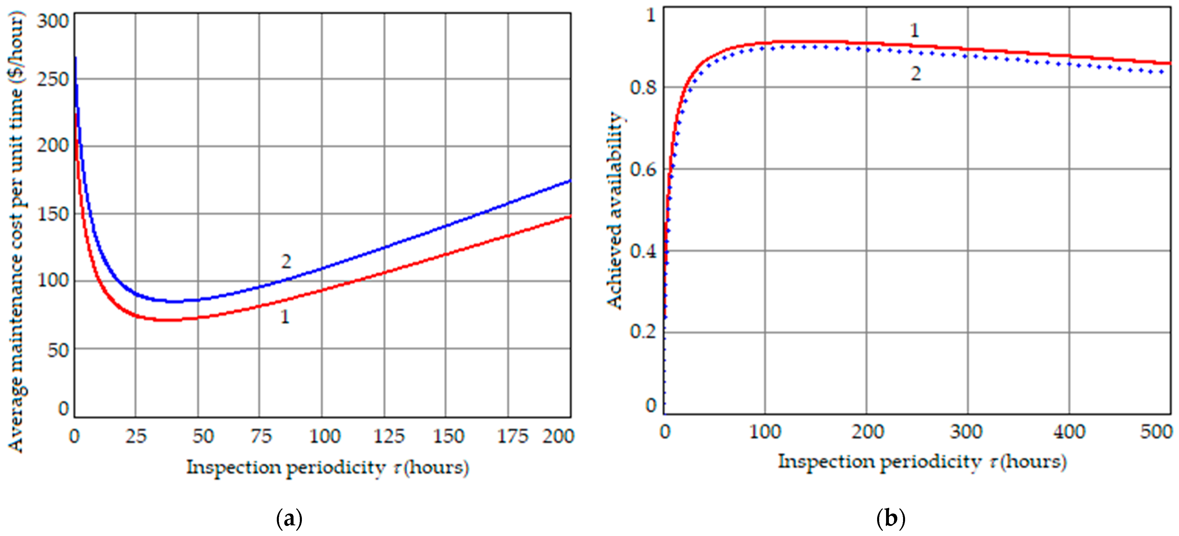
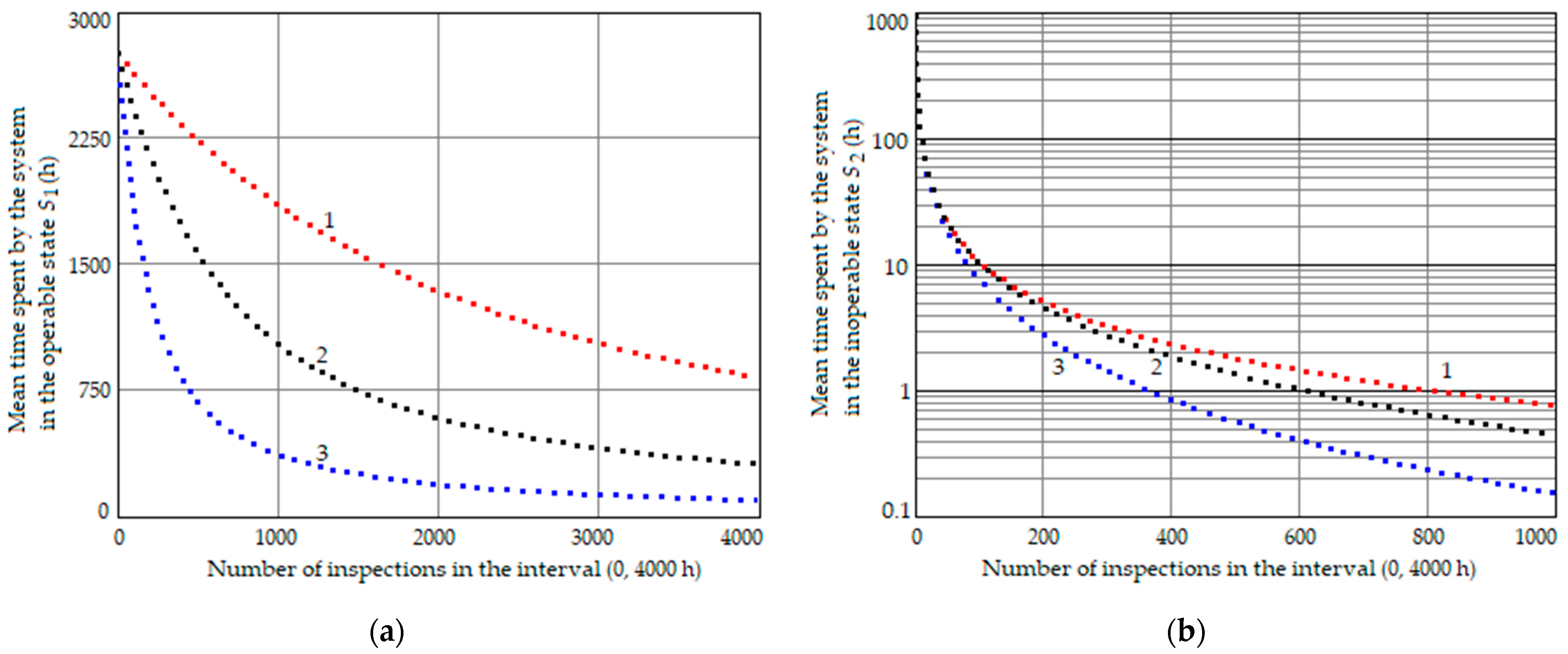
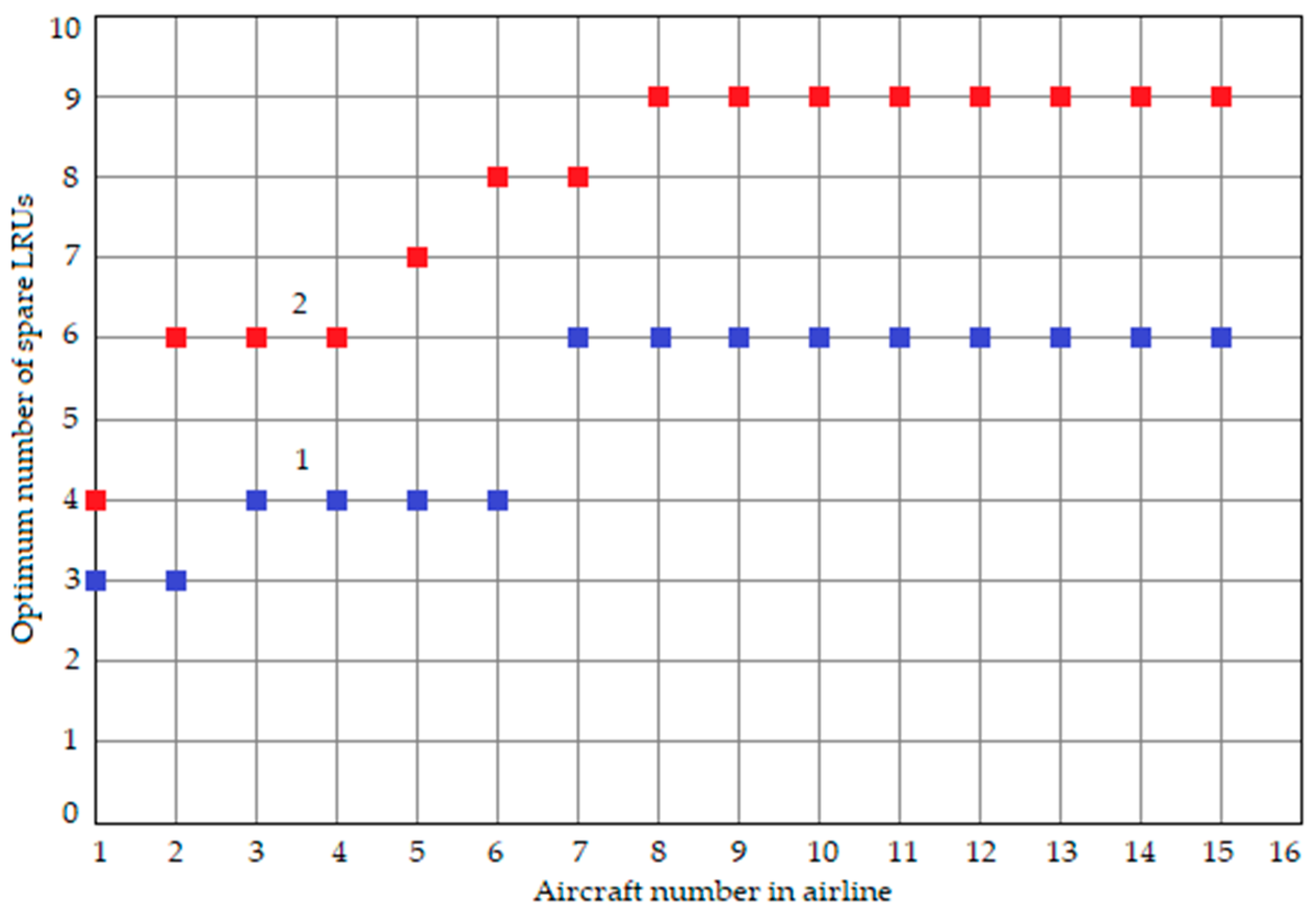3. Discussion

As outlined in Section 2, corrective and preventive maintenance models can be systematically classified into two categories contingent upon the conditional probabilities of false positives, true negatives, false negatives, and true positives: those characterized by constant probabilities and those marked by non-constant probabilities. When analyzing maintenance models with fixed and variable probabilities of correct and incorrect judgments, it is crucial to delve into the profound impact these probabilities exert on decision making processes. It is also essential to consider the validity of models to accurately predict system behavior and optimize maintenance strategies. Models with constant and nonconstant conditional probabilities of false positives and false negatives represent different approaches to capturing the uncertainties associated with maintenance decisions. Let us compare the validity of these models.

• Constant conditional probabilities of false positives and false negatives.

  1.1.

  Advantages.

  • Models with constant probabilities are often simpler to implement and analyze. They assume that the conditional probabilities of false positives and false negatives remain constant over time. Such maintenance models were analyzed in Section 2.1.
  • Constant probabilities of correct and incorrect decisions are relatively easy to estimate by simple Equations (136)–(139). It should be noted that these equations are utilized in most of the maintenance models with constant probabilities considered in Section 2.1.
  • Once the probabilities of errors are estimated, models remain stable and predictable, making it easier to plan maintenance activities.

  1.2.

  Disadvantages.

  • Constant error probabilities might not accurately reflect the complex nature of maintenance processes. In real-world scenarios, error rates can change due to various factors such as aging, usage patterns, and environmental conditions.
  • If error probabilities vary significantly over time (for instance, see Figure 6, Figure 9, Figure 10 and Figure 11), models with constant error probabilities can lead to inaccurate predictions and suboptimal maintenance decisions.
  • Constant probability models may result in either over-maintenance or under-maintenance, leading to inefficient resource utilization.

• Non-constant probabilities of false positives and false negatives.

  2.1.

  Advantages.

  • Non-constant error probabilities allow for a more realistic representation of maintenance processes. They can capture variations in error rates over time (see Figure 6, Figure 9, Figure 10 and Figure 11), accounting for factors like wear and tear, environmental changes, and operational conditions. Maintenance models with non-constant conditional probabilities of correct and incorrect decisions were considered in Section 2.2.
  • By incorporating changing error probabilities, these models can provide more accurate predictions, leading to better-informed maintenance decisions.
  • Non-constant error probabilities can adapt to different operating conditions, making models more versatile and applicable across diverse situations.
  • Non-constant probability models optimize resources by ensuring that maintenance activities are performed when needed, minimizing downtime, and reducing unnecessary maintenance costs.

  2.2.

  Disadvantage.

  • Models with non-constant error probabilities are generally more complex to develop and analyze. Estimating time-varying error probabilities might require appropriate modeling, statistical methods, and extensive data.

Let us now compare maintenance models where probabilities of false positives, true negatives, false negatives, and true positives are influenced solely by inspection timing versus models where these probabilities depend on both inspection timing and the moment of system failure.

• Maintenance models with probabilities of correct and incorrect decisions linked to inspection timing.

  1.1.

  Advantages.

  • Models based solely on inspection timing are often simpler to develop and implement. They rely on a straightforward relationship between inspection intervals and error probabilities. This class includes the maintenance models considered in [83,84,86,87,88,90,91,92,93,98].
  • Since error probabilities are primarily tied to inspection schedules, these models offer a degree of predictability, making it easier to plan maintenance activities.
  • Calculating error probabilities based on the time of inspections (periodic or sequential) is typically more straightforward and requires less complex data analysis.

  1.2.

  Disadvantages.

  • Ignoring the impact of system failures might lead to less accurate predictions of error probabilities. Real-world maintenance is influenced by both scheduled inspections and unexpected failures.
  • These maintenance models reveal that the probabilities of false positives, true negatives, false negatives, and true positives during multiple inspections are determined by multiplying the conditional probabilities of correct $(1-\alpha \left(t_i\right))$ and incorrect $(\alpha \left(t_{\nu }\right))$ decisions at different inspection times, as well as correct $(1-\beta \left(t_j\right))$ and incorrect $(\beta \left(t_n\right))$ decisions at other inspection times. Studies [27,29] have demonstrated that this multiplication approach is valid when the degradation stochastic process X(t) exhibits the property that, for a specific time to failure, there exists only one realization, denoted as x(t), of the random process X(t) that intersects with the failure threshold. Therefore, this class of maintenance models applies to a limited range of random degradation processes.

2.

Maintenance models with probabilities of correct and incorrect decisions that consider the time of inspections and the moment of system failure.

2.1.

Advantages.

• These models offer a more realistic representation of maintenance scenarios, considering the impact of scheduled inspections and unscheduled failures on the probability of errors. This class of maintenance models was considered in the studies [27,29,31,32,34,35,36,56,94,95,99,100,101,102,103,104].
• By considering a broader range of factors, these models can provide more accurate predictions, leading to better-informed maintenance strategies. Indeed, as illustrated in Figure 8 and Figure 10, the conditional probabilities of a true negative, false positive, true positive, and false negative depend not only on measurement accuracy and inspection time but also on the timing of the system failure. It is important to note that if the system fails immediately after the inspection time, each of the conditional probabilities of a true negative and a false positive at the time of the last inspection equals 0.5, assuming a symmetric PDF of error in estimating time to failure (refer to Figure 9a). Similarly, if the system fails just before the inspection time, each of the conditional probabilities of a true positive and a false negative at the time of the first inspection after failure equals 0.5 when using a symmetric PDF of error in estimating time to failure, as illustrated in Figure 9b. We also note that with a symmetric PDF of error in estimating time to failure, the maximum values of the conditional probabilities of a false positive and a false negative for a single inspection are equal to 0.5. It should also be noted that in the maintenance models considered in [27,29,31,32,34,35,36,56,101,102,104], the conditional probabilities of correct and incorrect decisions during multiple inspections consider both the moments of inspections and the moment of failure. Moreover, these probabilities also depend on the parameters of the degradation process.

2.2.

Disadvantages.

• Maintenance models incorporating multiple variables tend to be more complex. Estimating and analyzing the probabilities of correct and incorrect decisions considering inspection schedules, time of failure occurrence, and parameters of degradation processes in these models can be challenging, requiring sophisticated techniques and robust data.
• The accurate estimation of probabilities in these models may demand comprehensive data, both on the modeling of the degradation process and on historical failure patterns.

The choice between these maintenance models depends on the specific requirements applied to the maintenance planning and the available data. While models considering only inspection schedules in calculating error probabilities are simpler and more predictable, they may lack accuracy in capturing the complexities of real-world maintenance scenarios. Models considering both inspection timing and system failures in estimating error probabilities offer a more accurate and flexible approach, providing a closer representation of the actual maintenance process. However, these benefits come at the cost of increased complexity and data requirements. It is crucial to balance the trade-offs between simplicity and accuracy when selecting a maintenance model for a particular system.

4. Research Prospects in the Field of Maintenance Models with Non-Constant Probabilities of False Positives and False Negatives

The domain of maintenance models incorporating non-constant probabilities of false positives and false negatives encompasses probabilistic factors essential for predicting and overseeing the maintenance requirements of systems.

Future research can center on the advancement of dynamic modeling techniques capable of capturing variations in false positive and false negative probabilities over time. This could entail the integration of machine learning algorithms, Bayesian approaches, or other advanced statistical methods. Harnessing real-time or historical data to guide maintenance models holds significant promise. Through the analysis of large datasets by machine learning algorithms, patterns and trends in the probabilities of false positives and negatives can be identified, resulting in more adaptive and responsive maintenance strategies. The growing prevalence of Internet-of-Things devices and sensor technologies presents an opportunity to gather real-time data on system health. Research can concentrate on integrating such data into maintenance models, thereby enhancing the accuracy of probability estimates. Investigating the impact of human factors on maintenance decisions is another avenue of research. Understanding how human judgment and decision making interact with models that account for variable probabilities can lead to more effective implementation in real-world scenarios. The application of these models can extend beyond specific industries. Researchers may explore how maintenance models with non-constant probabilities can be adapted to various sectors such as manufacturing, transportation, nuclear stations, military equipment, and others.

5. Remarks

This survey aimed for a comprehensive scope. Nonetheless, any studies excluded were either deemed unrelated to the survey’s focus or unintentionally overlooked. We extend our apologies to both researchers and readers for any potential omission of relevant studies.