Article

Star-Identification System Based on Polygon Recognition

by
Gustavo E. Ramos-Alcaraz
1,
Miguel A. Alonso-Arévalo
1,* and
Juan M. Nuñez-Alfonso
2
1
Department of Electronics and Telecommunications, CICESE Research Center, Ensenada 22860, Mexico
2
UNAM Institute of Astronomy, Ensenada Campus, Ensenada 22860, Mexico
*
Author to whom correspondence should be addressed.
Aerospace 2023, 10(9), 748; https://doi.org/10.3390/aerospace10090748
Submission received: 30 June 2023 / Revised: 1 August 2023 / Accepted: 4 August 2023 / Published: 24 August 2023
(This article belongs to the Special Issue Advanced Small Satellite Technology)

Abstract

:
Accurate attitude determination is crucial for satellites and spacecraft. Among attitude determination devices, star sensors are the most accurate. Solving the lost-in-space problem is the most critical function of the star sensor. Our research introduces a novel star-identification system that utilizes a polygon-recognition algorithm to assign a unique complex number to polygons created by stars. This system aims to solve the lost-in-space problem. Our system includes a full solution with a lens, image sensor, processing unit, and algorithm implementation. To test the system’s performance, we analyzed 100 night sky images that resembled what a real star sensor in orbit would experience. We used a k-d tree algorithm to accelerate the search in the star catalog of complex numbers. We implemented various verification methods, including internal polygon verification and a voting mechanism, to ensure the system’s reliability. We obtained the star database used as a reference from the Gaia DR2 catalog, which we filtered, to eliminate irrelevant stars, and which we arranged by apparent magnitude. Despite manually introducing up to three false stars, the system successfully identified at least one star in 97% of the analyzed images.

1. Introduction

In ancient times, our ancestors identified patterns in the luminous objects of the night sky, which helped them to navigate and to move on land and sea. Due to the predictable nature of stellar motion, it has been possible to use this knowledge to consistently identify groups of known stars.
The tremendous increase in the launch of small and nanosatellites since 2020 [1] shows the great relevance of this type of technology, in regard to today’s immense challenges to sustainable development and human lifestyle. In 2022, companies and space agencies launched 2470 objects into space, compared to the 586 sent in 2019 [2]. These satellite launches represent an increase of 421% in just four years.
As for nanosatellites, despite the launches having decreased in number in 2019 and 2020, they have grown again in number since 2021. Over the past two years, 664 nanosatellites have been launched by organizations worldwide, which accounts for a 31% increase since the initial global launch [3].
In order for objects in Earth’s orbit, or traveling through space, to determine their location, they require a spatial reference. First, the attitude sensors help find the object’s orientation, also understood as where the object is pointing towards. Then, the attitude control subsystem manages and corrects the orientation, by using actuators, such as reaction wheels or magnetorquer [4].
Satellites rely on various sensors to accurately measure their attitude: the most commonly used are sun, horizon, magnetometer, and stars [5]. The star sensor shows a practical precision between 10–30 arcsecs in different implementations [6,7,8]. The fundamental limit of star sensor accuracy depends on the star distribution in our stellar neighborhood, star sensor dimensions, and exposure time. This theoretical precision can improve up to seven orders of magnitude or a few μ as (microarcseconds) [9].
There are two different types of problems that can be solved by a star sensor: lost-in-space and recursive algorithms [10]. The lost-in-space problem is of greater relevance, because it starts without any preliminary information on the object’s attitude. In the case of recursive algorithms, the algorithm may start working with information concerning some other type of attitude sensor or where the image sensor is pointing towards. This is why, in this case, the problem decreases a little in complexity. This paper deals with the development and actual testing of a lost-in-space algorithm that, like others of its kind, analyzes images over the entire sky vault without any initial orientation.
We can classify star-identification algorithms into two main types. The first variety uses isomorphisms of subgraphs. Here, the stars are considered vertices in a subgraph, with the angular distances between the stars as edge weights [11]. For the second variety, feature extraction and pattern search [12] are used. The stars are assigned a pattern, based on their position relative to neighboring stars, and they are then matched to the closest pattern in the database.
In 1997, Padgett et al. [11] proposed a pattern recognition method that assigned nearby stars within a certain radius for each pole star. The method then converted the pixel coordinates to larger binary regions and stored them in search vectors. This approach was novel, but needed to take advantage of search techniques.
The pyramidal identification technique developed by Mortari et al. [13] is a reference in subgraph isomorphisms. This method employs four stars as the vertices of a pyramid, then collects the interstar angles and stores them in a k-vector. The authors highlight the advantage of searching the created k-vector structure versus a binary search.
Li et al. [14] employ a technique that recursively searches for the identification of stars in a database by distances from the central star to its neighbors. For each iteration, they vote for any star if they find something, then verify and check the results. Thanks to their verification process, their technique exhibits robust and reliable performance.
Within the pole star algorithms, Wei et al. [15] present a novel technique aimed at enhancing the previous approaches of similar methods. They perform a radial search for each pole star, and they store the parameters of radius and distance from the pole star to each identified star inside the radius; they use this information to create search patterns with the neighboring stars. Then, they perform a verification phase, using a chain algorithm.
The methodology proposed in this article stems from the work conducted by Hernandez et al. [16] and Chavez et al. [17]. The method assigns stars as the vertices of polygons, and it employs a mapping function insensitive to similarity transformations. When tested with synthetic images, Hernandez et al.’s [16] algorithm demonstrated strong performance in simulations, thanks to its ability to withstand the rotation, scaling, and translation of the polygons formed by stars.
In this work, we present and evaluate a real-life implementation of a star-identification technique that solves the lost-in-space problem. The methodology is tested using catalogs generated with GAIA mission data in the DR2 release [18]. The star data has been filtered by apparent magnitude, variable stars, and stellar motion.
The proposed algorithm associates with a central star a number of polygons with a variable number of sides; neighboring stars are located at the vertices of the polygons. Our proposal uses a verification technique based on the use of several internal polygons and an overlapping FOV (field-of-view) voting scheme. In the presence of missing or false additional stars, our method is robust, in identifying changes in polygons of up to three vertices, by using more distant neighboring stars. We show a complete system with lenses, a camera (image sensor), a mini-processing machine, and software implementation.
The article has the following structure. In Section 2, we show the mathematical basis of the algorithm invariant to similarity transformations, binary searches, GAIA DR2 catalog generation, and star verifications. Section 3 presents algorithm performance evaluation techniques, such as synthetic catalog simulation with star generation, hardware and test bed, and image acquisition. In Section 4, we provide an analysis of the results and metrics. In Section 5, we provide some general conclusions about the work.

2. Description of Algorithm

Polygons are geometric figures constructed from a required number of line segments. One can assemble specific configurations of n-vertex polygons for each star pattern distinguished in an image of the night sky. These geometric figures allow us to extract data about the number of vertices, interior angles, exterior angles, and distance between vertices. It is possible to assign some of these characteristics or patterns to a unique value representing each constructed polygon, creating databases of polygons that can be searched or indexed more efficiently through a transformation function.

2.1. Creation of Star Catalog

The Hipparcos Catalog, named after the ancient Greek astronomer Hipparchus, is a high-precision star catalog from the European Space Agency’s Hipparcos satellite mission. It contains positions, parallaxes, and proper motions for over 118,218 stars [19]. The Tycho-2 Catalog, based on the same Hipparcos mission data, includes more than 2.5 million stars, offering a more extensive but slightly lower precision dataset [20]. The United States Naval Observatory (USNO) developed the USNO-B1.0 Catalog [21], which contains positions, proper motions, and magnitudes for over 1 billion stars, making it a valuable resource for astrometry and astrophysics research. The Gaia Archive, produced by another European Space Agency mission, aims to create the largest, most precise three-dimensional map of the Milky Way, by measuring the positions, distances, and motions of over 1 billion stars. The Gaia Archive DR2 (Data Release 2) data set contains 1.692 billion stars, of which 78.66% have the full astrometric solution. Some relevant parameters include positions in the sky ( α , δ ) , parallax, and proper motion (Gaia) [18].
In order to effectively manage our star catalog and optimize search results, we chose to utilize the GAIA DR2 data. This particular data set is currently recognized as the most precise, in terms of both coordinates and velocities. With the help of the “gaia archive” portal [22], we filtered the stars by relative magnitude, binary stars, variables, proper and radial motion, and parallax. As for relative magnitude, the main catalogs were created for magnitudes 5.5, 6, 6.5, and 7, as they are within the visual range of stars above the Earth’s surface. Binary and variable stars were eliminated from the catalog, so that they would not influence the identification process. We used the proper and radial motion and parallax to make an epoch change from the current epoch of the J2015.5 catalog to J2022.1. This process was carried out using the specialized software library Astropy [23]. The epoch change allowed us to correct and compensate for the displacement of some of the most-moving stars in the sky. We know from GAIA DR2 data that the average motion for stars with a magnitude less than 7 is 36 μ as (microarcseconds per year). However, some stars have 2–10 arcseconds per year: these cases can affect identification accuracy.
The position coordinates in GAIA DR2 are in the International Celestial Reference System (ICRS): this system originates in the solar system’s barycenter. The parameters are similar to those of equatorial coordinates. The RA coordinate represents the right ascension ( α ) , and the DEC coordinate shows the declination ( δ ) . These coordinates appear as points on a unit sphere with coordinates ( α , δ ) , as illustrated in Figure 1. The gnomonic projection is a method that maps the great circles of a sphere and translates the data of that half-sphere into a plane. Such projection is analogous to the result seen in a digitized image from a conventional CMOS (complementary metal—oxide–semiconductor) or CCD (charge-coupled-device) image sensor. Therefore, for each star in the catalog (central star with α 0 and δ 1 ) and those close to 180 , their coordinates ( α , δ ) are translated to a plane with coordinates ( x , y ) , as follows:
x = cos δ sin ( α α 0 ) cos c ,
y = cos δ 1 sin δ sin δ 1 cos δ cos ( α α 0 ) cos c ,
cos c = sin δ 1 sin δ + cos δ 1 cos δ cos ( α α 0 ) ,
where α 0 and δ 1 change in every iteration through the entire star catalog.

2.2. Invariant Algorithm

One of the usual problems when performing pattern recognition with real images is that the objects in search often change their scale, are rotated due to the position of the image sensor, or contain errors introduced by the acquisition hardware. For these reasons, it is often necessary to use an algorithm invariant to similarity transformations. The algorithm originally proposed by Chavez et al. [17] has been utilized in a star-identification algorithm tested using synthetic images [16]. The basis of this postulate is the following:
We are considering a fixed value for integers n 3 .
Definition 1. 
For any integer j = 1 , , ( n 1 ) / 2 , we consider the function φ j : C n C provided by:
φ j ( z 1 , , z n ) = k = 1 n λ j k z k k = 1 n λ j k z k ,
where λ = e 2 π 1 / n = e 2 ı π / n is an n-th root of unit, and ı is the unit imaginary number.
For each set of n-vertices with coordinates ( x , y ) in z k , we obtain a complex number φ j assigned to that specific polygon. The coefficients obtained in the numerator and denominator from Equation (4) are the Fourier descriptors or coefficients of the Discrete Fourier Transform: together with a basis of star-shaped polygons E k , it forms the linear combination of Z C n and is equal to k = 1 n x k E k . The work of Luque-Suarez et al. [24] gives full proof of the invariant algorithm and their original approach.
The nature of the invariant algorithm requires that the choice of the z k vertices follows sequential rules. The vertices of the polygons can support a cyclic shift or reverse order, as the outcome geometric figure would be precisely the same. However, we cannot guarantee the creation of the same invariant number φ j in case of a vertex permutation, rearrangement, or different choice selection. The rules are arbitrarily chosen, but should be followed consistently when creating the search catalog. For this work, they are as follows:
  • Choice of central star A;
  • Search for the nearest neighbor star to A, which is B.
  • Creation of a straight line between A and B, named AB.
  • Sorted from the smallest to the largest angle between the line AB and each of the other stars, measured counterclockwise.

2.3. Technique for Vertices Removal and Replacement

The elimination and substitution of stars (polygon vertices) allowed the algorithm to be robust to missing stars in the image to be analyzed. We created alternate catalogs containing extra information about neighboring stars.
The mathematical expression in Equation (5) describes the number of combinations of n objects taken r at a time without repetition [25]. For our purposes, this expression gives us the number of possible combinations of invariants. In this case, n is the number of elements removed in each combination, and r is the group of elements taken in each iteration. We observe that r = 5 1 = 4 , because the first component (1 or A) always remains fixed. In this work, we only show its operation with polygons of five vertices, this is illustrated in Figure 2. For polygons smaller than five vertices, it would not be possible to use the verification by internal polygons, because at least one triangle plus two vertices are needed. On the other hand, generating catalogs for vertices larger than five is possible; however, it increases the search time, because all invariants must be generated again for each catalog with different numbers of vertices. Therefore, using the expression (5), we obtain the total combination in Equation (6):
C n r = n r = n ! r ! n r !
C t o t a l = C 0 4 + C 1 4 + C 2 4 + C 3 4 = 1 + 4 + 6 + 4 = 15
The general star search involves a combination of invariants generated by different polygon configurations: each unique group of parameters is called a “set.” There are 15 invariants for each star, and four catalogs generated at different magnitudes (5.5, 6, 6.5, and 7). Thus, for each star, it is possible to find it in up to 60 different configurations.

2.4. Binary Search Method

To perform an efficient search, we applied the gnomonic projection and the invariant algorithm, and we selected appropriate vertices for each polygon or star in the catalog. From the point of view of a star-identification algorithm, we can simplify the problem to a similarity search between two catalogs: one with information from referential star databases (GAIA DR2, Hipparcos, or Tycho-2) C D , and the other catalog with data acquired through an imaging system, C I .
The C D and C I catalogs are constructed by the complex numbers φ , such that φ = a + b i . The imaginary and real parts can be represented in the complex plane, considering ( a , b ) as rectangular coordinates [ ( φ ) , ( φ ) ] . The structure of both catalogs is a matrix of size m × 2 , where m is the number of stars in each catalog. This structure can take advantage of the use of a binary search.
Among the binary search tree techniques, k-d tree is one of the dimensionality’s most widely implemented and versatile algorithms [26]. It creates clouds of points located at each node of the k-dimensional space, to search in each of its branches, subsequently. The method can achieve a search time of O ( log ( m ) ) if it does not have high dimensionality. In addition, it allows k-neighbor or radius searches. We can choose different search metrics: for the current matter, we describe a classical Euclidean distance metric d s t 2 in Equation (7), for the X and Y matrices between the vectors x s and y t , in the computational implementation of the k-d tree algorithm [27] in the MATLAB software:
d s t 2 = ( x s y t ) ( x s y t ) .

2.5. Verification Algorithm

The k-d tree search yields matching results that may contain false positives. This issue arises because noise-related variations in the star coordinates of the acquired images cause changes in the φ number. In addition, false and missing stars modify the creation of the polygons and generate a different φ number. Hence, we present a range of validation methods that, when coupled with the supplementary verification techniques, result in a robust and dependable implementation of the star-identification algorithm.

2.5.1. Verification by Internal Polygons

Our work involved creating five-vertex polygons that resembled the elements of P = A , B , C , D , E . Figure 3 illustrates this form, with A being the central star associated with the polygon. We ordered the elements in the same sequential form as P . To verify the polygon P , we ensured all its internal or inscribed polygons coincided between the C D and C I catalogs. The internal polygons, such as P 4 = A , B , C , D for polygons with four vertices and P 3 = A , B , D with three vertices, were included in this verification process.

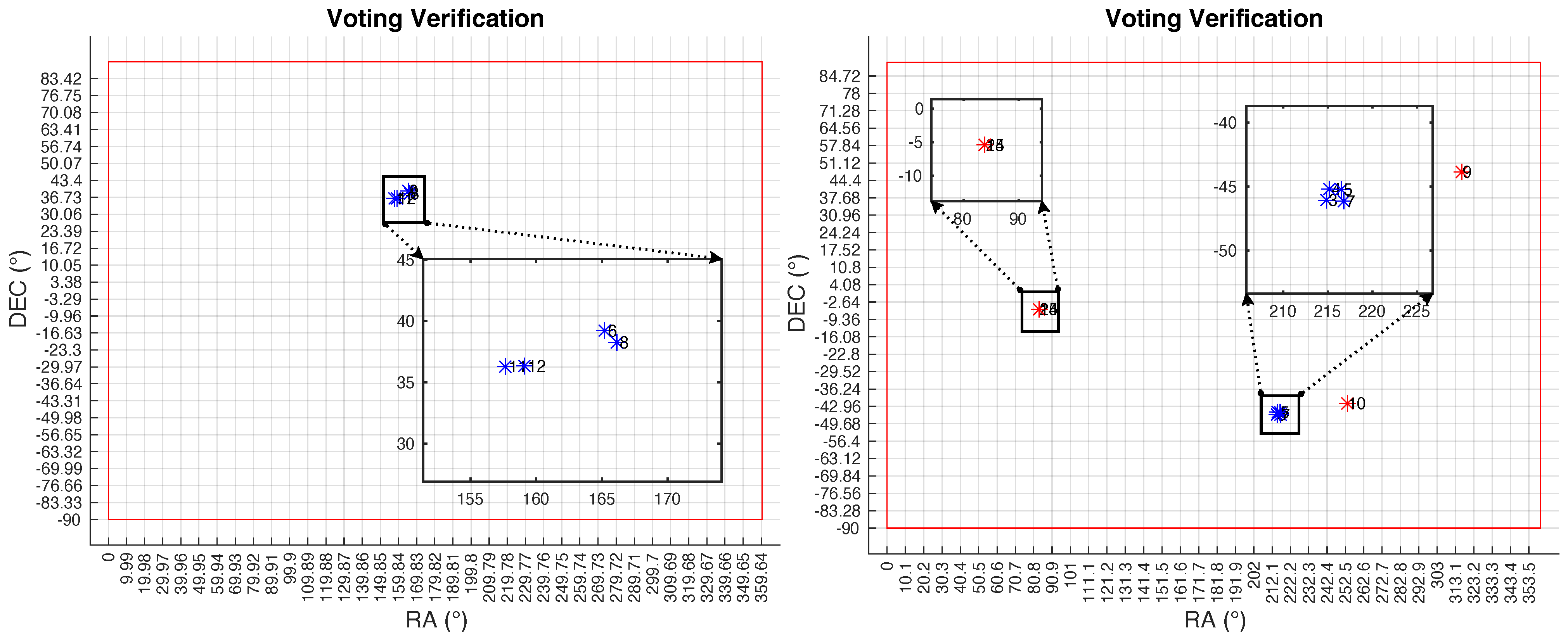
2.5.2. Voting Verification

In a star-identification algorithm, continuously encountering false positive results is one of the most critical problems to solve, affecting the star identification rate. This issue becomes crucial when working with real images of the night sky, as these contain more noise pixels than synthetic images generated by a computer. Due to this, we provide a star verification method based on regions of interest (ROI) and field of view (FOV). In this work, we show the ROIs as rectangles with red or blue lines according to the relevance of their enclosure region. Rectangles, known as regions of interest (ROIs), are used to surround each grouping of pixels that have enough brightness to be classified as a star. This method can process the data like data points instead of the entire image, making possible the highlighting of specific regions.
We have conceived a method that verifies and determines whether the matched regions of interest (ROIs) can be classified as identified stars. The method employs the field of view (FOV) of the captured images, and it implements a voting scheme that relies on the count of ROIs discovered within a designated sky region, to identify the image during the search. The procedure and rules are as follows:
  • For all stars found in the global search, the distance between their coordinates ( α , δ ) is obtained in a great circle.
  • They are grouped into regions with distances smaller than the FOV of the real image.
  • The method cannot decide, if it has found only one star.
  • If two stars are in the same region, the method verifies their identification; otherwise, it cancels both.
  • In groups with several stars in each, the group with the largest number is verified.

3. Implementation

This section shows the characteristics and specifications of the hardware devices we used to acquire and process the images and catalogs. In addition, we conducted an experimental procedure with the most crucial and necessary blocks, due to the implementation with real images.

3.1. Hardware and Test Bench Setup

Some commercial and professional star sensors—such as the T1 and T3 Star Tracker [6], Auriga-CP and Horus [7], and VST-68M and VST-41M [8]—have vast fields of view, ranging from 14 to 22 degrees. Commercial implementations of these systems cost approximately EUR 50–100,000; some are suitable for use in CubeSats or even small satellites. On the other hand, it is more complicated to find specific information about the optical sensors used, apart from the fact that most are CMOS. Based on the needs of each space mission, they select a suitable configuration that is energy-efficient and meets the requirements. Obtaining more stars with a larger FOV in the optical configuration is expected, making it possible to use smaller star catalogs [28]. However, striking a balance is necessary, as the pixel scale also depends on the image sensor used, and increasing this option can be challenging and costly. Another possibility involves changing the lens to one with different focal lengths; we discuss these options in Table 1.
The most straightforward optical system to implement a star identifier consists of two essential elements: lens and image sensor. For the lens, the main characteristics are focal length (F), diameter (or f-stop), and focusing range (in meters). The electronic imaging circuit technology for the image sensor can be CMOS- or CCD-type. Some crucial parameters are pixel size ( s p i x in μ m), resolution ( r x and r y coordinates in pixels), exposure time (in seconds), ADC (analog-to-digital converter resolution in bits), quantum efficiency (QE in % at the central wavelength λ c ), and full well (charge capacity per pixel in electrons, e ). Using Equation (8) [29], we can find the pixel scale θ p i x and, hence, the FOV for each lens and image sensor choice. The resulting FOV in the x axis will be F O V x = θ p i x × r x , and for the y axis, F O V y = θ p i x × r y . Choosing a longer focal length (F) lens makes the pixel scale ( θ p i x ) smaller, and the resulting image contains a smaller FOV of the sky. As for the image sensor, the resulting FOV grows in direct proportion to the pixel scale θ p i x :
θ p i x = 206265 × s p i x F [ arcsec / pix ] .
With this in mind, we analyzed the possibility of employing the ASI178MM [30] and ASI183MM [31] image sensors from the company ZWO. The company manufactures and distributes these devices as planetary cameras. However, their use in astrophotography is well known, due to the relation between quantum efficiency, full well capacity, and read noise against their quality and cost. Regarding the lens, we considered two options based on what was available in the laboratory where we were working: a Celestron AVX 6 inches Schmidt–Cassegrain telescope [32] of F = 1500 mm and a Kowa LM75HC lens [33] of F = 75 mm.
In the context of capturing images of the night sky in a city with some light noise, Table 1 presents the key specifications of a lens and camera, with a focus on their performance in low-light conditions. Although there are some similarities in certain parameters between these two cameras, such as full well and pixel size, it is important to consider their differences, with respect to other cameras. The full well capacity represents the amount of electrical charge each pixel can withstand until it becomes filled. When this happens, the information related to that pixel is lost and can cause blooming in adjacent pixels. In both cameras, the value is 15k e . The pixel size is also the same in both cameras, being 2.4 μ m. Therefore, the difference in FOV and pixel scale is directly related to the higher pixel count and sensor size of the ASI183MM and to the focal length of the lenses.
Another important factor to consider is the quantum efficiency of each sensor: the ASI183MM overall has a QE greater than 3% versus the ASI178MM. The manufacturer’s charts [30,31] show that their peak efficiency is located in the green band, at roughly 500 nm and 550 nm for ASI178MM and ASI183MM, respectively. It is important to note that our GAIA DR2 catalogs used the “PHOT_G_MEAN_FLUX” as a filter, based on magnitude. This value corresponded to the average flux in the green band (G) [34]. Due to the need for a larger FOV and better quantum efficiency, the system chosen for imaging was the one with the ASI183MM camera and LM75HC lens. Figure 4 displays the complete optical arrangement previously described.

3.2. Image Acquisition Process

We created a database of our images, to test the algorithm’s behavior and implementation. The primary goal was to replicate the specifications and conditions of a star sensor as accurately as possible. These conditions included using the imaging equipment in the field or out of the lab.
To accomplish this, we utilized an optical arrangement that linked the LM75HC lens to the image sensor identified as ASI183MM. As for the computer to acquire the images, we performed the tests using two machines: the first was a laptop with Windows 11 and i5-11400h processor, with which we could perform sessions of about 2–4 h of battery life; the second machine was a MiniPC, the Aero2Pro, with a Celeron N5105 processor. This MiniPC had the advantages of a small form factor, low power consumption, and low cost, which benefits a configuration for longer session duration. Different conditions can utilize each configuration.
We initially conducted multiple sessions for image acquisition testing, to fine-tune the optical system parameters. To capture a wide range of sky regions, we conducted multiple imaging sessions between October 2022 and June 2023, to compile our main catalog. We gathered a total of 100 pictures of the sky, taken from all directions, without any limitations. We conducted both sessions at the top of the hill, which is where CICESE, our research institution, is located. Figure 4 shows our setup. The precise coordinates are 31°52′21.5″ N 116°40′11.8″ W, in Ensenada, Baja California, Mexico. We selected this site because, despite its position on the outskirts of the city, it offered minimal interference from light pollution and noise, which could have negatively impacted the quality of our captured images. In this spot, the light from the city is obstructed on one side of the sky, resulting in a slight reduction in light pollution. However, the quality of the images was still affected by the city’s light pollution and the illumination of the Institute facilities.
Using ASI Studio software, we acquired the images at a full resolution of 5496 × 3672 pixels. Although the software allowed for it, no pixel binning was applied, because we wanted to obtain the highest-possible pixel resolution. The camera software was configured with an exposure time of 0.5 s and standard gain. To focus on a very distant point, we set the lens with a focus at infinity and an aperture with an f-number of f / 4 . In Figure 5, we can see one of these images with a logarithmic adjustment in the SAOImage DS9 software [35]. From here, we noticed not only a large amount of background noise appearing but also many regions that potentially were stars.
The first method we use to estimate the amount of noise in the image and to be able to discern between relevant and unnecessary information is a histogram of the raw data. In Figure 6, we see a typical example of histogram values: on the x-axis is the pixel value (16-bit, from 0 to 65,535) with a log 2 scale and “nbins” equal to the length of all possible values. On the y-axis, the histogram graph shows the number of repetitions for each data. From here, we can know the most frequent values in the image, which are usually the background noise we want to eliminate. Based on these values, we center the image noise on the maximum value of the histogram, H m a x .

3.3. Experimental Procedure

Regions of interest (ROIs) form rectangles around each contiguous blob or cluster of pixels that have enough illumination to be considered a star. This technique allows for highlighting a particular region and, thus, processing the data by sections and not the whole image. The importance of using a small region of interest is well known, due to pixel inhomogeneity and noise. Likewise, the size must ensure the star signal is within the window [36].
There are several algorithms for object identification by regions of interest. He et al. [37] mentions four basic types of algorithms that perform region identification by scans: double-scan; multiscan; hybrid; and tracking algorithms. Osuna [38] adds to the methods the single scan [39], compares its performance for a star sensor. considering the simplicity and computational cost, and concludes that the double scan is the best for this situation. The description of the double-scan algorithm is as follows [38]:
  • Each image pixel is analyzed from left to right and then from top to bottom.
  • For each pixel considered as an object (other than 0), the mask of Figure 7 is applied, and the labels already assigned are analyzed. The current pixel in work is represented by I ( x , y ) .
  • If a label already exists within the mask, it is replaced in the pixel, and if several labels are assigned, the smallest one is taken.
  • A second scanning assigns the labels to the neighbors.
Figure 8 shows the result after applying the double-scan algorithm to identify the ROIs. We established two minimum-threshold pixel values, to determine whether a region was important. The first one was the fixed threshold T f ( T f = 5 pixels): this pixel value was kept constant for all the analyzed images, since there would always be very faint or dim star values below it. We adjusted the second threshold value, a dynamic parameter, based on the background noise of each image ( H m a x of the histogram) and the iteration in which we were searching for a certain amount of ROIs: we called it the dynamic threshold T d , and we adjusted it using a bisection algorithm.
The bisection algorithm is a simple iterative procedure converging to a solution that is known to fall within an interval [ a , b ] [40]. In this situation, a and b were the number of ROIs identified in each iteration of the double-scan algorithm. Therefore, we initially set a value of ROIs that we wanted, e.g., 10–15 regions.
Consequently, evaluating the function at the midpoint,
x = a + b 2 .
Furthermore, we tested in which subintervals the solution lay:
a , a + b 2 , a + b 2 , b .
The identification algorithm iterated and searched in a finite cycle (30 cycles maximum), until it found sufficient ROIs. If it did not find enough regions, we aborted the image identification, considering there was too much noise in the image. Figure 9 shows a typical example of this method and how in seven iterations it managed to find a sufficient number of regions where 10 < ROIs < 15 .
A star in a real image manifests as a pixel blob; therefore, locating its center with the naked eye is impossible. The pixel illumination disperses around the star’s center, to resemble a Gaussian elliptical scattering source [41]. For this reason, it is necessary to find the centroid of the image pixel blob. Some of the most commonly used centroid calculation algorithms are center-of-gravity (CoG) [42], weighted-first-moment [43], and symmetric-Gaussian-fitting [44]. We decided to employ the center-of-gravity algorithm, due to its robustness and low computational complexity, which leads to little processing time. It can be applied directly to the two-dimensional array or to the margin of the obtained distribution [42].
Equations (11) and (12), which took the ROI to a centroid coordinate ( x c , y c ) depended on the positions of each pixel ( x i j , y i j ) ; the pixel luminosity was ( I i j ) ; n and m were the numbers of pixels on each axis of the ROI:
x c = i = 1 n j = 1 m x i j I i j i = 1 n j = 1 m I i j
y c = i = 1 n j = 1 m y i j I i j i = 1 n j = 1 m I i j
Following the polygon formation rules in the “Algorithm description” section, we created polygons associated with each star of the real image. The centroid coordinates ( x c , y c ) identified each star in the catalog and real image. In Figure 10, we worked out the case in a region with 10 stars in the real image, and we then generated the 10 unique polygons. The red star was the central star A, joined sequentially to the following four stars by a blue line.
Another critical step in creating invariant catalogs is to make the work robust against pixel position errors in real images. As already employed by [16] in synthetic catalogs, we introduced noise as uniformly distributed pseudorandom integers, U [ a , b ] , where [ a , b ] was the minimum and maximum pixel noise to each coordinate of the polygon vertices, and we iterated this process for 100 cycles. The goal was to include a margin of error in the invariant database C D , to match this with the real image invariant C I .
For a single ABCDE polygon, as in Figure 3, a noise catalog C N with 100 elements, as described in the set of Equation (13), was created. Equation (14) shows the process of selecting minima φ min and maxima φ max invariant bounds for each set of C N elements. Finally, Figure 11 demonstrates the distribution of these noise coordinates surrounding the invariant, where the blue dots display the dispersion of the invariant values with noise, and the red dots define the bounds of the new region assigned to the invariant. We repeated this process for each star in our GAIA DR2 catalogs. Although it could take some time for all the 5.5-, 6-, 6.5-, and 7-magnitude catalogs, it did not exceed 15 min on the previously described laptop, and it only needed to run once:
C N = P 1 ( x A , y A ) ± U , , ( x E , y E ) ± U , , , P 100
( φ min , φ max ) = min [ φ ( C N ) ] , max [ φ ( C N ) ]
We searched between the C I and C D invariant catalogs of complex numbers φ C I and φ C D using the k-d tree algorithm [27]. Some critical conditions for a fast search are that the number of columns must be less than 10, the input data must not be sparse, and the metric distance must be Euclidean. If any of these conditions are unmet, the algorithm is switched to an exhaustive search. In the basic configuration, the software assigns 50 data points per node in every bucket and, thus, generates all the necessary buckets. Algorithm 1 explains the steps that decide and identify the algorithm. A search tree is created with two columns, each with a complex number component and each row corresponding to each star. We performed a range search from a point to the box ( φ min , φ max ) . Then, we checked the identification with the inscribed polygons P 4 and P 3 .
Algorithm 1 Match invariants φ with the kd-tree search algorithm
  for each φ in C I  do
     if (RangeSearchkd-tree( φ C D ) in point φ C I ) ≠ 0 then
       match = φ C D matched invariants
       if (RangeSearchkd-tree(match( P 4 , P 3 )) in point φ C I ( P 4 , P 3 )) ≠ 0 then
          match = update matches
          print verified stars
       end if
     end if
end for

4. Experimental Results

This section shows the search results for invariants between the C I and C D catalogs, and the search methods and experimental verification with which we tested our catalog of 100 night sky images.

4.1. Matching Regions for Polygons with Three, Four, and Five Vertices

Once we had candidate invariants to identify a star, we needed to proceed to the verification process. As described in previous sections, we had several verification algorithms with which to filter and decide to match an ROI with a C D star. In Figure 12, we carried out this procedure for one of the real images in our catalog, starting the verification process from the image on the right and moving to the left. In the image on the right, we started by observing a case where the ROI invariant (blue asterisk) fell inside the red error box in search of the C D invariant: this was for polygons of five vertices. Then, the algorithm removed one of the vertices and searched again in the invariants catalog. In the central Figure, we see again how box number 16 surrounded ROI #2. Finally, in the left image, we confirmed that the three-vertice polygon had been identified with the same box and ROI. Therefore, we concluded that the verification method by internal polygons had corroborated the identification of region number 16 with ROI #2.

4.2. Voting Verification Results

Voting verification was the process that established the rules by which we decided whether or not to recognize each ROI as a star. Figure 13 shows two of our images (47 and 41 of Table A1 in Appendix A). On the left, we observed how the four ROIs, previously verified by the internal polygon algorithm, had been grouped according to their RA and DEC coordinates. We detected that the region where the ROIs were located was smaller than the FOV of the acquired images; therefore, we verified through this method that we had found the four stars to which ROIs 6, 8, 11, and 12 belonged. On the right, we see a situation where we had grouped ROIs 3, 4, 5, and 7, but where we had separated ROIs 2, 9, 10, 14, and 15 into different regions. This drawback arose due to the collision of the complex numbers of the invariants against other invariants, which can cause false positives in the identification. Our approach may result in overlapping invariant regions associated with two or more stars. In this work, we referred to this overlap as a collision between the invariant regions of two or more stars. However, we see how this voting method managed to eliminate these false ROIs and find the true ones based on our proposed rules.

4.3. Results of Identification in Our Catalogs

Below, we show the results of the star identification process in our catalog of the 100 night sky images we acquired. In Appendix A, Table A1 and Table A2 contain complete information on the ROIs, the verification algorithm by internal polygons, verification by voting, and manual validation. We present a summary of average values and standard deviations in Table 2. The number of identified stars present in every image was examined: in Table 2, this parameter is called “Identified Images”. Through experimentation and analysis of the images, we found that the results varied according to the number of identified ROIs. Thus, we display this comparison for three different threshold ranges of ROIs: these values were 15–20, 21–30, and 31–40 ROIs. We must remember that the algorithm solves this selection of ROIs iteratively between the configured parameters, so choosing the proper minimum and maximum values is crucial for better performance. If we reduced the number of ROIs below 15, the algorithm did not generate enough polygons, and the performance degraded significantly.
It was reasonable to assume that expanding the number of ROIs would result in a proportional increase in the identified ROIs. The important realization here was that even with the threshold between 21–30 ROIs, we could eliminate certain regions if they were within a short distance of one other: this was why the number of identified ROIs remained below the threshold or range, with 12.74, 17.5, and 23.49 being the respective average value for each group. The results of the star-identification algorithm in base form ranged between an average of 4.31, 7.61, and 10.5 ROIs identified per group. The voting verification method decreased the average number of identified ROIs by an average of 0.96–2.09, as it filtered out some regions. To safely guarantee the validity of our results, we added a “manual validation” where we could see the actual results. To realize this process, we uploaded the 100 images to the astronomical image calibration platform Astrometry.net [45]. Our image database is open to the public for research and academic purposes in the following online album [46]. From here, we extracted the image coordinates according to the new plate solving applied to it by this website, and we compared them to the FOV resulting from our algorithm. The results of the manual validation closely matched those obtained through the verification method, as demonstrated in Table 2 and Figure 14. For the group with even fewer ROIs, it was the same. However, the two larger groups were slightly separated by an average of 0.24–0.37, indicating that a minimal amount of stars were misidentified. Finally, we observed that the final result of the identification process grew with the more ROIs there were in the search group—starting at an accuracy of 71%, continuing at 88%, and achieving a notable 97% value. It is worth noting that the program’s running time increased as we consider a greater number of ROIs. An invariant search for a specific polygon configuration, using the Windows-based laptop mentioned above, took slightly below 50 ms under Matlab.

4.4. Performance and Results with Addition of False Stars

In order to test the performance of the algorithm in the specific case of false stars, we added up to three fake ROIs to one of our images (image 61 of Table A2). These false stars were placed at coordinates ( x , y ) for P 25 = ( 3000 , 2500 ) , P 26 = ( 2000 , 2000 ) , and P 27 = ( 1000 , 3000 ) . In Figure 15, we see the result of this test; the blue asterisks represent the ROIs potentially identified as stars, while the red ones represent those not identified. We can compare this result to using only the base algorithm without the voting verification. The location of these false stars was strategic, because we wanted them to be close to the regions we were identifying, so that they would be more likely to affect the identification of the real contiguous stars. However, the result shows that this was not the scenario, and that the algorithm managed to eliminate the three points correctly.

4.5. Relationship to Earlier Work

As previously mentioned, the methodology presented in this article originates from the work proposed by Hernandez et al. [16], using the polygon-recognition algorithm developed by Chavez et al. [17]. However, these works did not propose a real star-identification system like the one presented in this article. To be more specific, Hernandez et al.’s [16] research solely focused on simulated star images, and it did not account for the possibility of missing or false stars, making it less reliable. The present work is a major improvement, because it solves the limitations and proposes a complete star-identification system, including an optical subsystem, support hardware, and algorithm implementation. Furthermore, the identification system was evaluated, using authentic star images.

5. Conclusions

In this paper, we propose a star-identification system based on polygon recognition. We form polygons with stars at their vertices. For this purpose, we employ an algorithm that assigns a unique complex number to each polygon, by which these geometric figures can be identified in complex number catalogs. In order to solve the lost-in-space problem, we decided to obtain a bank of images of the night sky, trying to make them similar to those that a star sensor in space would find. Although the observing conditions were not the most suitable, we obtained a catalog of 100 good-quality images containing enough data to test the star-identification algorithm. We realized the need for a verification mechanism, so we added the verification methods by internal polygons and verification by voting. We obtained images, and we compared them to a star database obtained from the catalog Gaia DR2 and processed through epoch changes, filtered from non-relevant stars, and organized by apparent magnitude. Using the complete system, we could identify at least one star in up to 97% of the analyzed images.
The verification methods contribute significantly to the robustness of the algorithm against perturbations. The proposed system has been tested with up to three false stars; however, the algorithm was not affected by adding false stars, and it continued correctly identifying real stars in that same FOV.
A limitation of the current algorithm is establishing an adequate range of ROIs, through which sufficient polygons are formed to perform the invariant search between the image catalog and the star database. Increasing the FOV of the optical system would implicitly help obtain a larger number of more luminous stars and, thus, improve the system’s performance. The current code implementation has been an essential proof of concept, and we could obtain faster identification using an algorithm implemented in a lower-level language.

Author Contributions

Conceptualization, G.E.R.-A.; methodology, G.E.R.-A. and M.A.A.-A.; software, G.E.R.-A.; validation, G.E.R.-A.; formal analysis, M.A.A.-A. and J.M.N.-A.; investigation, G.E.R.-A.; resources, M.A.A.-A. and J.M.N.-A.; data curation, G.E.R.-A.; writing—original draft preparation, G.E.R.-A.; writing—review and editing, M.A.A.-A. and J.M.N.-A.; supervision, M.A.A.-A.; funding acquisition, M.A.A.-A. All authors have read and agreed to the published version of the manuscript.

Funding

The work of Gustavo E. Ramos-Alcaraz was supported by the Mexican National Council on Science and Technology (CONACYT) of Mexico through the scholarship under Grant 842163.

Data Availability Statement

The data presented in this study are available on request from the corresponding author.

Acknowledgments

The authors thank the anonymous reviewers for their valuable comments and suggestions that helped improve the manuscript’s quality and those who have directly or indirectly provided assistance to support this project.

Conflicts of Interest

The authors declare no conflict of interest.

Abbreviations

The following abbreviations and symbols are used in this manuscript:
FOVField of view for each optical setup
ROIRegion of interest
GAIA DR2Data Release version 2 of the space mission Gaia
α RA, barycentric right ascension in ICRS system
δ DEC, barycentric declination in ICRS system
φ j The invariant complex number associated with every polygon
C D Catalog of invariant complex numbers from GAIA Database polygons
C I Catalog of invariant complex numbers from our real-images polygons
P Polygons created with five, four, and three stars in the vertices
H max The maximum value of the histogram
T f Threshold fixed value for considering a region of pixels to be relevant
T d Threshold dynamic value that adjusts with bisection algorithm
C N Noise catalog with 100 invariants for each polygon
φ min and φ max Region or box with minimum and maximum of the C N

Appendix A

Appendix A.1. Tables of Results of the 100 Images Acquired

This appendix shows the identification results in each stage and the verifications for the 100 night sky images we acquired. The results and discussion analyze and complement the raw data shown here.
Table A1. Part 1 (1–52 images). Identification results. ROIs = recognized ROIs after the filter method by the nearest centroids. A.-Id. Stars = algorithm-identified stars after the internal polygons verification. V1 = verification of stars by voting method. V2 = manually validated stars. Id. (Yes/No) = final identification process after the verification steps. Every digit from the “XYZ” corresponds to the results from 15–20, 21–30, and 31–40 ROIs. 1 = Identified, and 0 = Not Identified.
15–20 ROIs21–30 ROIs31–40 ROIs
No. ImageROIsA.-Id. StarsV1V2ROIsA.-Id. StarsV1V2ROIsA.-Id. StarsV1V2Id.
(Yes/No)
1121101622121141010001
2137221453327131212111
3157442011111124141212111
4148881588824141313111
51311101017141313221298111
660001132213220010
795331352213522111
8106441064410644111
9130001711131131111001
10113332143321433111
111632220433261077111
12107551911101023141111111
13101102140040833001
14158771976625161414111
15144441912121223121212111
16104222215141428151313111
171465519128831171616111
18174331866623877111
19142212284422844011
20161112032227777011
21133222397723977111
22178772418151229161212111
231311101019141382716159111
241852218522311187101
25113221897622877111
26136551843318433111
2791112440124421001
281376617109923161111111
29118771598815988111
30141010103017151531181616111
31159992312111127121010111
32146662111111131201616111
33114441554425922111
34148881712111123151515111
35148881610101024181616111
36138661743324181313111
37112211614131323181616011
38139991811111124171515111
3970001343324988011
40124442012111120121111111
411100017944201066011
42127552212121222121212111
431144419121111291377111
44122221553319101010111
45110001486617966011
461000015107719866011
47124331544420855111
48114441876529141010111
4912665168772311109111
50125551544418333111
51113211566215993111
52104441377715777111
Table A2. Part 2 (53–100 images). Continuation of the identification results.
15–20 ROIs21–30 ROIs31–40 ROIs
No. ImageROIsA.-Id. StarsV1V2ROIsA.-Id. StarsV1V2ROIsA.-Id. StarsV1V2Id.
(Yes/No)
531142116131091712119111
5411763148722113135111
55143221432221632111
561200015533231188011
571211017300261199001
58159772012111127141111111
59114331453324444111
60125422295522995111
611565518118824111111111
62124221575523722010
63123221353316533111
6481111344421987011
651444416444231088111
66145331742124121111111
67143332113111124121212111
681686619131111271399111
691343318777241299111
701411016222291388011
7192111400020322001
72195211952219521111
73224222242222422111
741000015311231499001
75120002354423544011
76154221743324999111
771376616108824171313111
78125332220202022202020111
7914110171088301277011
80139881798821988111
81122221576625866111
82120001200018321000
83188771887731733111
84146551465525855111
85139991710991710109111
86110001721128555001
871555518877271188111
88112211562221755001
89163222484434171313111
90131002064125544001
91123012012121229201818011
92111001666626161515011
93132221776617766111
94118771486620322111
95111011775517755011
96154331543315433111
97101001952228633011
98179882215141426181515111
991343317555241299111
100146551465524955111

References

  1. Lavender, A. Satellites Orbiting the Earth in 2022. 2022. Available online: https://www.pixalytics.com/satellites-in-2022/ (accessed on 28 June 2023).
  2. UNOOSA. United Nations Office for Outer Space Affairs, Online Index of Objects Launched into Outer Space. 2023. Available online: https://www.unoosa.org/oosa/osoindex/search-ng.jspx?lf_id= (accessed on 28 June 2023).
  3. Kulu, E. World’s Largest Database of Nanosatellites, over 3600 Nanosats and CubeSats. 2023. Available online: https://www.nanosats.eu (accessed on 28 June 2023).
  4. Grøtte, M.E.; Gravdahl, J.T.; Johansen, T.A.; Larsen, J.A.; Vidal, E.M.; Surma, E. Spacecraft Attitude and Angular Rate Tracking using Reaction Wheels and Magnetorquers. IFAC-PapersOnLine 2020, 53, 14819–14826. [Google Scholar] [CrossRef]
  5. Liebe, C. Pattern recognition of star constellations for spacecraft applications. IEEE Aerosp. Electron. Syst. Mag. 1992, 7, 34–41. [Google Scholar] [CrossRef]
  6. Terma-Company. Star Trackers for Various Missions. 2022. Available online: https://www.terma.com/products/space/star-trackers/ (accessed on 28 June 2023).
  7. SODERN-Ariane-Group. World Leader in Star Trackers. 2023. Available online: https://sodern.com/en/viseurs-etoiles/ (accessed on 28 June 2023).
  8. VECTRONIC-Aerospace-GmbH. Star Trackers VST-68M, VST-41M. 2023. Available online: https://www.vectronic-aerospace.com/star-trackers/ (accessed on 28 June 2023).
  9. Fialho, M.A.A.; Mortari, D. Theoretical Limits of Star Sensor Accuracy. Sensors 2019, 19, 5355. [Google Scholar] [CrossRef]
  10. Spratling, B.; Mortari, D. A Survey on Star Identification Algorithms. Algorithms 2009, 2, 93–107. [Google Scholar] [CrossRef]
  11. Padgett, C.; Kreutz-Delgado, K. A grid algorithm for autonomous star identification. IEEE Trans. Aerosp. Electron. Syst. 1997, 33, 202–213. [Google Scholar] [CrossRef]
  12. Rijlaarsdam, D.; Yous, H.; Byrne, J.; Oddenino, D.; Furano, G.; Moloney, D. A Survey of Lost-in-Space Star Identification Algorithms Since 2009. Sensors 2020, 20, 2579. [Google Scholar] [CrossRef] [PubMed]
  13. Mortari, D.; Samaan, M.A.; Bruccoleri, C.; Junkins, J.L. The Pyramid Star Identification Technique. Navigation 2004, 51, 171–183. [Google Scholar] [CrossRef]
  14. Li, J.; Wei, X.; Zhang, G. Iterative algorithm for autonomous star identification. IEEE Trans. Aerosp. Electron. Syst. 2015, 51, 536–547. [Google Scholar] [CrossRef]
  15. Wei, X.; Wen, D.; Song, Z.; Xi, J.; Zhang, W.; Liu, G.; Li, Z. A star identification algorithm based on radial and dynamic cyclic features of star pattern. Adv. Space Res. 2019, 63, 2245–2259. [Google Scholar] [CrossRef]
  16. Hernández, E.A.; Alonso, M.A.; Chávez, E.; Covarrubias, D.H.; Conte, R. Robust polygon recognition method with similarity invariants applied to star identification. Adv. Space Res. 2017, 59, 1095–1111. [Google Scholar] [CrossRef]
  17. Chávez, E.; Chávez Cáliz, A.C.; López-López, J.L. Affine invariants of generalized polygons and matching under affine transformations. Comput. Geom. 2016, 58, 60–69. [Google Scholar] [CrossRef]
  18. ESA. European Space Agency. Gaia Data Release 2 (GAIA DR2). 2018. Available online: https://www.cosmos.esa.int/web/gaia/dr2 (accessed on 28 June 2023).
  19. Perryman, M.A.C.; Lindegren, L.; Kovalevsky, J.; Hoeg, E.; Bastian, U.; Bernacca, P.L.; Crézé, M.; Donati, F.; Grenon, M.; Grewing, M.; et al. The Hipparcos Catalogue. Astron. Astrophys. 1997, 323, L49–L52. [Google Scholar]
  20. Høg, E.; Fabricius, C.; Makarov, V.V.; Urban, S.; Corbin, T.; Wycoff, G.; Bastian, U.; Schwekendiek, P.; Wicenec, A. The Tycho-2 catalogue of the 2.5 million brightest stars. Astron. Astrophys. 2000, 355, L27–L30. [Google Scholar]
  21. Monet, D.G.; Levine, S.E.; Canzian, B.; Ables, H.D.; Bird, A.R.; Dahn, C.C.; Guetter, H.H.; Harris, H.C.; Henden, A.A.; Leggett, S.K.; et al. The USNO-B Catalog. Astron. J. 2003, 125, 984–993. [Google Scholar] [CrossRef]
  22. ESA. European Space Agency, Gaia Archive. 2023. Available online: https://gea.esac.esa.int/archive/ (accessed on 28 June 2023).
  23. Astropy Collaboration; Price-Whelan, A.M.; Lim, P.L.; Earl, N.; Starkman, N.; Bradley, L.; Shupe, D.L.; Patil, A.A.; Corrales, L.; Brasseur, C.E.; et al. The Astropy Project: Sustaining and Growing a Community-oriented Open-source Project and the Latest Major Release (v5.0) of the Core Package. Astrophys. J. 2022, 935, 167. [Google Scholar] [CrossRef]
  24. Luque-Suarez, F.; López-López, J.L.; Chavez, E. Indexed Polygon Matching Under Similarities. In Similarity Search and Applications; Reyes, N., Connor, R., Kriege, N., Kazempour, D., Bartolini, I., Schubert, E., Chen, J.J., Eds.; Series Title: Lecture Notes in Computer Science; Springer International Publishing: Cham, Swtizerland, 2021; Volume 13058, pp. 295–306. [Google Scholar] [CrossRef]
  25. Brualdi, R.A. Introductory Combinatorics, 5th ed.; Pearson/Prentice Hall: Upper Saddle River, NJ, USA, 2010. [Google Scholar]
  26. Bentley, J.L. Multidimensional binary search trees used for associative searching. Commun. ACM 1975, 18, 509–517. [Google Scholar] [CrossRef]
  27. Celestron-LLC. Classification Using Nearest Neighbors. 2023. Available online: https://www.mathworks.com/help/stats/classification-using-nearest-neighbors.html (accessed on 28 June 2023).
  28. Leake, C.; Arnas, D.; Mortari, D. Non-Dimensional Star-Identification. Sensors 2020, 20, 2697. [Google Scholar] [CrossRef]
  29. Berry, R.; Burnell, J. The Handbook of Astronomical Image Processing, 2nd ed.; Willmann-Bell: Richmond, VA, USA, 2005. [Google Scholar]
  30. ZWO-Company. ASI178MM (Mono). 2023. Available online: https://astronomy-imaging-camera.com/product/asi178mm-mono/ (accessed on 28 June 2023).
  31. ZWO-Company. ASI183MM (Mono). 2023. Available online: https://astronomy-imaging-camera.com/product/asi183mm-mono/ (accessed on 28 June 2023).
  32. Celestron-LLC. Advanced VX 6″ Schmidt-Cassegrain Telescope. 2023. Available online: https://www.celestron.com/products/advanced-vx-6-schmidt-cassegrain-telescope (accessed on 28 June 2023).
  33. Kowa-Optimed-Deutschland-GmbH. LM75HC 1″ 75 mm 5MP C-Mount Lens. 2023. Available online: https://www.kowa-lenses.com/en/lm75hc–5mp-industrial-lens-c-mount (accessed on 28 June 2023).
  34. ESA. European Space Agency, Gaia Data Release Documentation. 14.1.1 Gaia Source. 2021. Available online: https://gea.esac.esa.int/archive/documentation/GDR2/Gaia_archive/chap_datamodel/sec_dm_main_tables/ssec_dm_gaia_source.html (accessed on 28 June 2023).
  35. Joye, W.A.; Mandel, E. New Features of SAOImage DS9. In Proceedings of the Astronomical Data Analysis Software and Systems XII, Strasbourg, France, 12–15 October 2003; Volume 295, p. 489. [Google Scholar]
  36. Liebe, C. Accuracy performance of star trackers—A tutorial. IEEE Trans. Aerosp. Electron. Syst. 2002, 38, 587–599. [Google Scholar] [CrossRef]
  37. He, L.; Chao, Y.; Suzuki, K.; Wu, K. Fast connected-component labeling. Pattern Recognit. 2009, 42, 1977–1987. [Google Scholar] [CrossRef]
  38. Osuna, M.H. Image Processing Algorithms for Star Centroid Calculation: Small Satellite Application. Master’s Thesis, CICESE, Ensenada, México, 2017. [Google Scholar]
  39. AbuBaker, A.; Qahwaji, R.; Ipson, S.; Saleh, M. One Scan Connected Component Labeling Technique. In Proceedings of the 2007 IEEE International Conference on Signal Processing and Communications, Dubai, United Arab Emirates, 24–27 November 2007; IEEE: Dubai, United Arab Emirates, 2007; pp. 1283–1286. [Google Scholar] [CrossRef]
  40. Weisstein, E.W.; Bisection. From MathWorld–A Wolfram Web Resource. 2023. Available online: https://mathworld.wolfram.com/Bisection.html (accessed on 28 June 2023).
  41. Delabie, T.; Schutter, J.D.; Vandenbussche, B. An Accurate and Efficient Gaussian Fit Centroiding Algorithm for Star Trackers. J. Astronaut. Sci. 2014, 61, 60–84. [Google Scholar] [CrossRef]
  42. Samaan, M.A. Toward Faster and More Accurate Star Sensors Using Recursive Centroiding and Star Identification. Ph.D. Thesis, Texas A&M University, College Station, TX, USA, 2003. [Google Scholar]
  43. Nightingale, A.M.; Gordeyev, S. Shack-Hartmann wavefront sensor image analysis: A comparison of centroiding methods and image-processing techniques. Opt. Eng. 2013, 52, 071413. [Google Scholar] [CrossRef]
  44. Stone, R.C. A Comparison of Digital Centering Algorithms. Astron. J. 1989, 97, 1227. [Google Scholar] [CrossRef]
  45. Lang, D.; Hogg, D.W.; Mierle, K.; Blanton, M.; Roweis, S. Astrometry.net: Blind Astrometric Calibration of Arbitrary Astronomical Images. Astron. J. 2010, 139, 1782–1800. [Google Scholar] [CrossRef]
  46. Astrometry.net. Album of Images: GustavoRamosStarIDInvariant. 2023. Available online: https://nova.astrometry.net/albums/4273 (accessed on 28 June 2023).
Figure 1. Graphical representation of a gnomonic projection. This projection type moves points grouped on the hemisphere to their respective place on a plane. The yellow mini-spheres would be the stars in the sky, and the points on the plane would be the projection on the image sensor.
Aerospace 10 00748 g001
Figure 2. Vertices removal and replacement technique. We form the initial polygon with the stars at vertices A B C D E ; then, we replace these stars with the three extras. The symbol ★ indicates the positions of the stars in FOV.
Aerospace 10 00748 g002
Figure 3. Here is an example of how to form a polygon with five vertices. We place a star at each vertex and use the internal or inscribed polygons to confirm correctly identifying the initial polygon. We create polygon P 4 = A , B , C , D with the red and P 3 = A , B , D with the green dotted lines.
Aerospace 10 00748 g003
Figure 4. On the (left) are the LM75HC lens and ASI183MM camera. On the (right), we show the complete assembly of the optical system and the location where we set up the image acquisition session.
Aerospace 10 00748 g004
Figure 5. Image of the night sky captured using the mentioned configuration. The image has undergone minimal processing, with only a logarithmic adjustment made to the brightness values, in order to emphasize possible star regions.
Aerospace 10 00748 g005
Figure 6. In this raw night sky image histogram, we observe the location of the immense amount of background noise.
Aerospace 10 00748 g006
Figure 7. Utilized mask in the double-scan algorithm; the current pixel is I ( x , y ) .
Aerospace 10 00748 g007
Figure 8. In red are the ROIs that exceeded the T d , and in blue are those that exceeded the T f but fell below the T d . Finally, light spots did not meet even the minimum T f .
Aerospace 10 00748 g008
Figure 9. Timeline of ROIs found and iterations.
Aerospace 10 00748 g009
Figure 10. Examples of how the polygons assigned to each star are formed, with the first vertex being the red star. The measurements for both the horizontal and vertical units are in terms of pixel coordinates.
Aerospace 10 00748 g010
Figure 11. This plot shows a region of invariant’s noise with 100 iterations. The noise introduced at each real and imaginary coordinate is uniformly distributed pseudorandom integers.
Aerospace 10 00748 g011
Figure 12. Tracking matching regions in which an invariant can be identified through verification in matching boxes for three, four, and five vertices. The blue asterisks represent the invariants of the polygons formed with the stars present in the image. The red rectangles represent the boundary regions for each invariant in the catalog C D .
Aerospace 10 00748 g012
Figure 13. Images 47 and 41 of our image catalog in Table A1. Blue asterisks represent the ROIs that the internal-polygon verification algorithm approved. Red asterisks represent those ROIs located outside the FOV.
Aerospace 10 00748 g013
Figure 14. Comparison of the results in different stages of identification and verification. We observed growth in the number of ROIs and identification as soon as we used a threshold region with more ROIs.
Aerospace 10 00748 g014
Figure 15. Example of the star identification performance for image 61 of Table A2. Stars found by the base algorithm are in * blue, and those not identified are in red. On the right, we enclose three ROIs representing noise in red ovals.
Aerospace 10 00748 g015
Table 1. We analyzed four optical configurations of image sensors and lenses.
SettingsASI178 & 6 SCTASI178 & L75ASI183 & 6 SCTASI183 & L75
Sensor size (inches)1/1.81/1.811
Pixel size ( μ m)2.42.42.42.4
Resolution (pixels)3096 × 20803096 × 20805496 × 36725496 × 3672
ADC (bits)14141212
QE (%)81% at λ c = 500 nm81% at λ c = 500 nm84% at λ c = 550 nm84% at λ c = 550 nm
Focal length (mm)150075150075
Pixel scale (arcsec/pix)0.336.60.336.6
Radial FOV (degrees)0.1913.8130.3376.732
Table 2. Results of the identification process according to the various verification steps.
ROIsAlg.-Identified StarsVoting VerificationManual ValidationIdentified
Threshold in ROIsMean σ Mean σ Mean σ Mean σ Images
15–2012.742.484.312.953.352.833.352.8371
21–3017.53.317.614.036.214.145.974.1088
31–4023.294.8510.54.518.414.418.044.4797
σ = Standard deviation.
Disclaimer/Publisher’s Note: The statements, opinions and data contained in all publications are solely those of the individual author(s) and contributor(s) and not of MDPI and/or the editor(s). MDPI and/or the editor(s) disclaim responsibility for any injury to people or property resulting from any ideas, methods, instructions or products referred to in the content.

