A Study on Thermal Management Systems for Hybrid–Electric Aircraft

Abstract

The electrification of an aircraft’s propulsive system is identified as a potential solution towards a lower carbon footprint in the aviation industry. One of the effects of increased electrification is the generation of a large amount of waste heat that needs to be removed. As high-power systems must be cooled to avoid performance deterioration such as battery thermal runaway, a suitable thermal management system is required to regulate the temperature of the powertrain components. With this in mind, the main objective of this research is to identify promising heat transfer technologies to be integrated into a thermal management system (TMS) such that power, mass, and drag can be minimised for a parallel hybrid–electric regional aircraft in the context of the EU-funded FutPrInt50 project. Five different TMS architectures are modelled using the Matlab/Simulink environment based on thermodynamic principles, heat transfer fundamentals, and fluid flow equations. The systems are a combination of a closed-loop liquid cooling integrated with different heat dissipation components, namely ram air heat exchanger, skin heat exchanger, and fuel. Their cooling capacity and overall aircraft performance penalties under different flight conditions are estimated and compared to each other. Then, a parametric study is conducted, followed by a multi-objective optimisation analysis with the aim of minimising the TMS impact. As expected, none of the investigated architectures exhibit an ideal performance across the range of the studied metrics. The research revealed that, while planning the TMS for future hybrid–electric aircraft, alternative architectures will have to be developed and studied in light of the power requirements.

1. Introduction

The aviation sector is currently facing new challenges such as energy demand and environmental impact. The report Flightpath 2050 set several goals that must be accomplished by the year 2050 [1], including a reduction of 75% in terms of CO${}_2$ emissions. In this context, sustainable multidisciplinary design optimisation is rapidly becoming a key factor in the development of next-generation aircraft [2].

In this multidisciplinary analysis, the interaction of propulsion and energy fields is of particular interest. Even though using electric powertrains and cleaner energy sources as a propulsive system seems to be a promising solution, it still needs to surpass several technological hurdles [2,3,4,5,6,7]. One of these barriers is related to the fact that more electric aircraft have increased demands on engines for thrust and power generation, leading to hotter fluids, higher component temperatures, and increased heat generation [8]. Although electrical equipment is typically efficient, the large amount of electrical power needed (in the Megawatt range) will result in significant power losses [9]. Additionally, the heat created by the electric propulsion system cannot be taken through the engine nozzles and the use of ram air to cool electric systems is limited due to their greater integration into the fuselage [4]. There is also an increased risk of thermal runaway with some systems, especially batteries [10]. Thus, novel thermal management systems (TMSs) are required and should be considered from the conceptual design stages [11]. The TMS will be responsible for regulating the temperature of the aircraft subsystems/components by managing heat transfer between heat sources and heat sinks in order to optimise comfort, safety, and efficiency [12]. Therefore, the major design goal of a TMS is to minimise its impact on the aircraft in terms of important metrics such as weight, power consumption, and drag, while allowing for the diverse components and systems to run within a safe temperature range.

Within this framework, the FutPrint50 project stands out as a critical endeavour aimed at discovering and developing technologies and combinations that will help to speed up the entry-into-service to 2035/2040 of a commercial regional hybrid–electric aircraft (HEA) [13]. The main goal of this research work, as a FutPrInt50 collaboration, is to study new and existing heat dissipation systems and develop possible TMS architectures. This will help to understand the influence of a TMS on the power, weight, and drag as well as shed light on the feasibility of these architectures in future aircraft.

The remainder of this article is organised as follows: (i) first, a literature review on heat transfer technologies for TMS architectures is provided in Section 2; (ii) Section 3 builds upon it and five different architectures are proposed alongside each of their constituent components; (iii) then, a parametric study followed by a multi-objective optimisation process are presented in Section 4, where the architectures are compared; and (iv) finally, the main remarks on this work are drawn in Section 5.

2. Literature Review

2.1. Overview of Heat Transfer Technologies

The thermal management system acquires heat at the heat source, transports and rejects it at the heat sink [9]. Understanding the heat source behaviour is thus essential since it influences TMS requirements. Heat sources are any component or system that generates heat, either as a by-product or as its main function. Electrified propulsion systems are expected to generate additional heat loads besides conventional heat loads generated by combustion engines, mechanical power transmission, and the environment control system (ECS). Main electric powertrain heat sources may include electric motors/generators, batteries, fuel cells, and power converters/distributors. The thermal management system will be responsible for the heat transfer to the heat sink. Heat exchangers, liquid cooling loops, and refrigeration cooling loops, namely vapour compression systems (VCSs), can be used in this stage. Atmospheric air and fuel are the main terminal heat sinks in aircraft, and for this reason they are presented next.

2.1.1. Atmospheric Air

Ram air (RA), engine fan air (EFA), and skin heat exchanger (SHX) are technologies that use atmospheric air as a heat sink. RA systems use the dynamic pressure caused by the movement of the aircraft to ingest air into a duct that can be charged directly to cool down the devices or that can be transferred to ram air heat exchangers (RHXs) to cool down a coolant. In RA inlets, the air is brought to a halt relative to the aircraft which causes drag. An SHX system uses the aircraft surface as a thermal interface to the atmospheric air heat sink. This reduces air inlets, minimising RA system cooling drag [14].

2.1.2. Fuel

Aircraft fuel is easily transported, making it a possible heat sink. Moreover, hydrocarbon fuels have, in general, better heat transfer properties than air, making them a more effective cooling fluid [9]. At the same time, there is a thermodynamic advantage of preheating fuel before combustion, as it results in a more efficient thermal cycle. However, using fuel also has its drawbacks, including fuel thermal stability and fuel thermal endurance, which can affect aircraft safety. Thus, reducing the amount of heat load transferred to the fuel thermal management system (FTMS) itself and improving its thermal behaviour is of extreme importance to ensure flight safety and prevent accidents, such as the TWA Flight 800 [15], from happening. Nevertheless, in the ultimate case of a fully electric aeroplane, no fuel will be available on board.

2.2. Overview of TMS Architectures

Most of the technologies previously described are used in the current research on TMSs for electrified aircraft propulsion. The main design challenge to improve the overall TMS performance is how to create such a system wherein the heat loads are the mostly efficiently transported through cooling loops and dissipated at the existing heat sinks.

Table 1. Research TMS architectures.

Aircraft (PAX)	Cooling System	Refs.
ECO-150R (150)	RA and liquid	[16]
STARC-ABL (154)	EFA, RA, fuel, liquid (oil + PGW30/PSF-5), and SHX	[17,18]
PEGASUS (48)	RA, liquid (PGW30/PSF-5), and SHX	[17,18]
SUSAN (180)	RA, fuel, liquid (PGW30/PSF-5), and SHX	[19]
ULI (76)	RA, ECS air, and liquid	[20]
Short-range aircraft (180)	RA Fuel tank with internal heating and SHX	[21,22]
Notional aircraft	FTMS (single and dual tank topology)	[23,24]
N + 3 (180)	RA, liquid, and VCS	[25]

sums up some of the most important studies on the TMS integration conducted recently [16,17,18,19,20,21,22,23,24,25]. These studies suggest that liquid cooling, RA cooling, outer mould line cooling, heat exchangers, and the use of fuel as a heat sink are the most promising heat transfer systems, although VCS usage is also explored. Most of the TMS configurations studied were based on liquid–RA cooling loops. A coolant with a high thermal capacity is required. The use of sustainable aviation fuel (SAF) instead of Jet-A both in the powerplant and as a heat sink can also bring advantages. Firstly, since it is a “drop-in” fuel, i.e., it can be combined with conventional fuels, it only requires minor adjustments in the powerplant. Secondly, life cycle carbon emissions can be reduced [26].

The focus of this paper, developed under the scope of the FutPrInt50 project, was mainly two-fold: (i) to develop TMS models that can be incorporated into the conceptual design of the next generation of hybrid–electric regional airliners at a low computational cost to enable multidisciplinary design optimisation; and (ii) to provide a comparison between the different TMS architectures considered in the aforementioned project. These models were conceived and implemented from the scratch for regional hybrid–electric aircraft. To the best of our knowledge, no other work in the open literature was found covering these two aspects.

3. Methodology

This section is structured as follows: in Section 3.1, the reference aircraft and corresponding mission profile are established; Section 3.2 presents the TMS architectures alongside the assumptions taken to enable the parametric and optimisation studies; Section 3.3 provides the mathematical formulation for modelling each component of the TMS architectures to allow for repeatability; the verification of these models is shown in Section 3.4; in Section 3.5, the computational procedure to simulate the architectures is exemplified for architecture 5; and the multi-objective optimisation problem is formulated together with the implementation details in Section 3.6.

3.1. Reference Aircraft and Mission

The baseline propulsion architecture used to design and size the TMS is a parallel hybrid architecture with two turboprop engines running on SAF and coupled to an electric motor each, which can also be powered by battery packs [13]. Wingtip propellers driven by electric motors are also part of the powerplant. In this work, the main characteristics of the considered reference aircraft were the ones initially studied in the project, which are listed in

Table 2. Main characteristics of the reference aircraft alongside those of the ATR42-600 (data from [29]).

Parameter (Units)	Reference Aircraft	ATR42-600
Maximum Take-Off Mass (kg)	18,000	18,600
Cruise Speed (km/h)	520	556
Cruise Altitude (m)	7010	7010
Wing span (m)	27	24.57
Wing area (m${}^2$)	54.5	54.5
PAX (−)	50	48

alongside those of the ATR42-600 used in [27]. This latter aircraft was chosen as the category benchmark in the project [28].

A first estimation of some general aircraft dimensional parameters was conducted to obtain some reference measures for the fuel tank and ducts, components used in the TMS architectures. An overview of the aircraft outer mould line design is presented in Figure 1.

Figure 2 outlines the considered mission profile, which is a simplified one that accounts for a range of 400 km, a cruise speed of 520 km/h, and a cruise altitude of 7010 m.

The TMS should regulate the temperature of the different components in the described powerplant, namely batteries, electric motors, and power electronics. Other subsystems were disregarded since the computational models developed in this paper are focused on conceptual aircraft design. Nevertheless, in a later design stage, it would be important to consider coupling the TMS with the environmental control system (ECS), as pointed out in [30] to benefit from synergistic effects and mitigate the performance impact on the aircraft.

With this in mind, the total waste heat load generated by these components and their operating temperatures was estimated. An initial estimation showed a critical heat load value of 237 kW during take-off (TO). However, in a previous study by the authors [27], this value was found to be lower than 200 kW for the ATR42-600 with a parallel hybrid–electric propulsion system and the characteristics displayed in Table 2. This latter aircraft is slightly different, namely its propulsive system does not have the wingtip propeller-driven electric motors, albeit it includes two additional electric motors. Two of them act as generators to convert the power of each turboshaft into electricity that is used to power the two propeller-driven electric motors. In the cited work, even though the focus was on the propulsion system, its coupling with a TMS that accounted for different components (namely batteries, electric motors, generators, and power electronics) was also considered. For this reason, we assumed a maximum heat load of 200 kW. Since the TMS will be designed to manage half of the total heat load according to the symmetry of the hybrid–electric propulsion (HEP) architecture, an assumed value of 100 kW is considered as a representative heat load (${\dot{Q}}_{\mathrm{equip}}$). The operating temperature of the battery pack limits the heat load intake liquid temperature (control temperature). The battery working nominal temperature (305 K) is defined as the control temperature ($T_{\mathrm{control}}$).

3.2. TMS Architectures

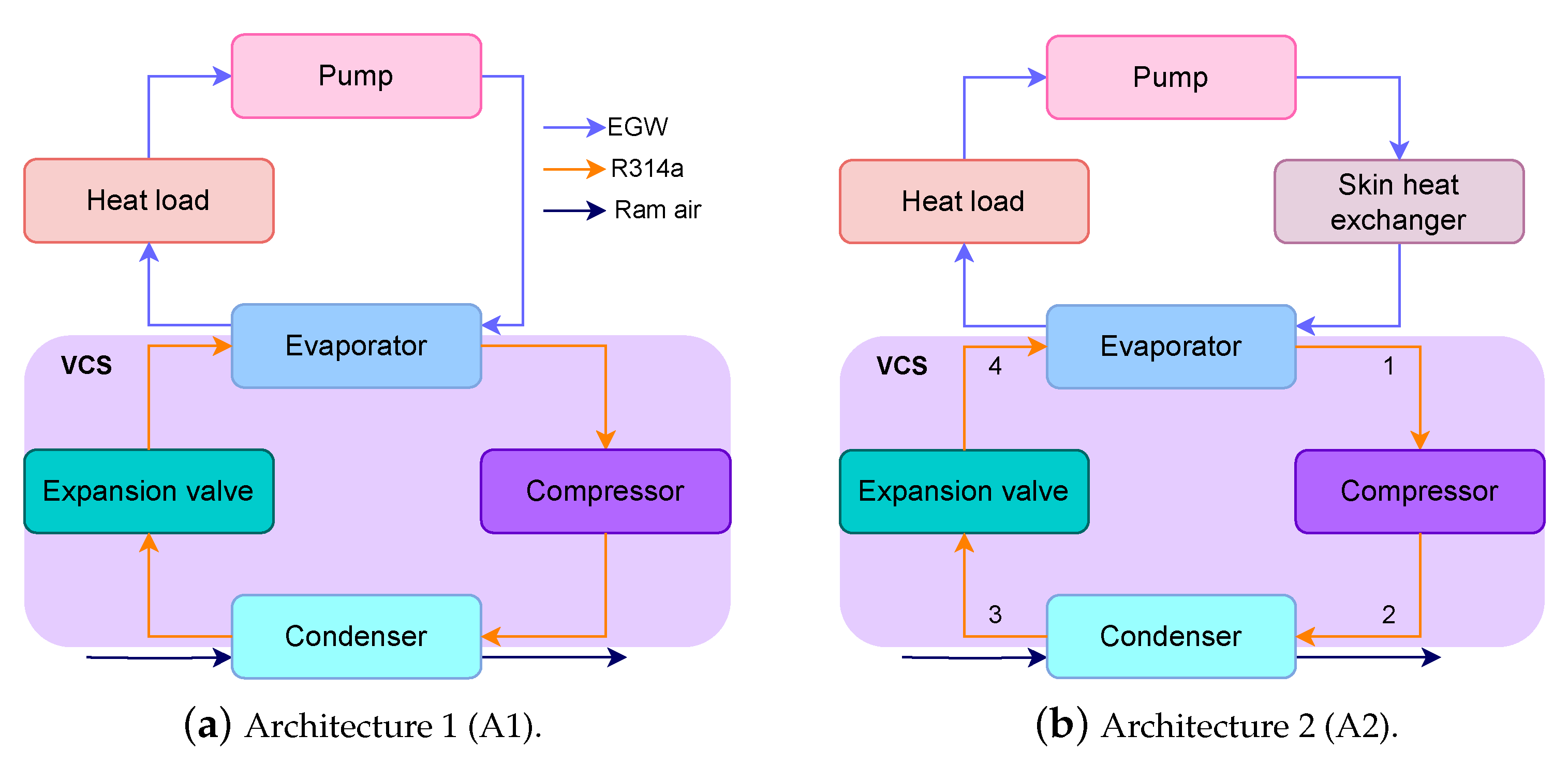
Five TMS architectures were formulated based on two factors: (i) a literature review conducted by the authors [30]; and (ii) an early architecture proposed by Embraer for the FutPrInt50 project [31], which corresponds to Architecture 2 in the current paper. SHX and fuel as heat sink, besides conventional liquid cooling loops, VCS, and ram air heat exchangers were identified in the cited work as the subsystems worth considering at a conceptual level given their higher technological readiness levels. With these systems in mind, we devised these five architectures. Architecture 1 (A1) and Architecture 2 (A2) both use a liquid cooling loop, a VCS, and an RA inlet to cool the equipment. The difference between the two is that, in A1, the heat is only removed via the evaporator to the VCS, while, in A2, before transferring heat to the VCS, the liquid rejects heat to the ambient air through an SHX. A1 and A2 layouts are presented in Figure 3.

Architecture 3 (A3) and Architecture 4 (A4) use a liquid cooling loop and RA inlet to cool the equipment. In A3, the liquid cooling loop only includes a liquid–ram air heat exchanger (RHX), while in Architecture 4, before rejecting heat to an RA mass flow, the liquid transfers heat to the ambient air through an SHX. A4 and A3 layouts are presented in Figure 4.

Architecture 5 (A5), depicted in Figure 5, differs from the others since it also uses fuel as a heat sink. To use liquid–fuel as a heat sink, an FTMS is developed and the fuel is heated via a fuel heat exchanger (FHX) and cooled using the SHX concept.

In this work, two main assumptions were made: (i) the heat load from the equipment is set constant to the peak load; and (ii) quasi-steady state simulations are considered in detriment to time-consuming unsteady ones. The former is a conservative approach as the peak load was never exceeded in a previous study by the authors [27] for a similar hybrid–electric aircraft with a parallel layout. Also, this allows for the observation of key features of the different components in the TMS architectures throughout the mission profile. Moreover, the model here described is possible to use with a variable heat load, as achieved in [27]. Regarding the usage of quasi-steady simulations instead of unsteady ones, despite affecting the results from our point of view, it does not negate the comparison between TMS architectures, one of the main focal points of the current work. Moreover, the difference from unsteady simulations can be mitigated by increasing the number of flight mission points. Furthermore, this latter assumption was one of the FutPrInt50 project assumptions since its integration in a full aircraft optimisation process [32] was needed at a smaller computational cost.

3.3. Component Model

The model equations for thermal balance and mass estimation were developed for each component that integrates the TMS architectures using Matlab/Simulink.

3.3.1. Heat Load

Heat load represents all the equipment to be cooled and it is provided to the system as a heat transfer rate ${\dot{Q}}_{\mathrm{equip}}$. The first law of thermodynamics (principle of conservation of energy) applied to a control volume with fluid crossing its boundary adapted to a simplified steady-flow thermal system may determine the coolant output temperature [33]:

$${\dot{Q}}_{\mathrm{equip}}={\dot{m}}_{\mathrm{liquid}}·c_p·(T_{\mathrm{liquid},\mathrm{o}}-T_{\mathrm{control}}),$$

(1)

where $c_p$ is the specific heat at constant pressure and T the liquid temperature. The i and o subscripts distinguish between fluid entry and exit, respectively. To compute the liquid mass flow rate (${\dot{m}}_{\mathrm{liquid}}$), a norm from a Society of Automotive Engineers report is used [34]. For liquid cooled avionics, flow rates range from 0.023 kg/s to 0.045 kg/s per kW and are usually considered for coolants such as ethylene–glycol water (EGW) mixtures.

3.3.2. Coolant and Fuel Pumps

EGW pumps and fuel pumps compensate for the circuit pressure drop ($\Delta p$) from the EGW and fuel passage through the ducts, heat loads, and heat sinks, respectively. Assuming a constant efficiency (${\eta }_{\mathrm{pump}}$) and knowing the fluid density (${\rho }_{\mathrm{liquid}}$), the pump power consumption $W_{\mathrm{pump}}$ may be estimated as follows:

$$W_{\mathrm{pump}}=\frac{{\dot{m}}_{\mathrm{liquid}}·\Delta p}{{\rho }_{\mathrm{liquid}}·{\eta }_{\mathrm{pump}}}.$$

(2)

3.3.3. Heat Exchangers

The primary variables in a heat exchanger (HEX) are its heat transfer rate ${\dot{Q}}_{\mathrm{HEX}}$ (W), surface exchange area $A_{\mathrm{HEX}}$ (m${}^2$), heat capacity rates $C\left(\dot{m}·c_p\right)$ (W/K), and total heat transfer coefficient U (W/Km${}^2$). To determine the heat transfer rate, the steady flow energy equation is applied on hot and cold fluid sides and combined to an extension of Newton’s law of cooling using the global heat transfer coefficient U and an adequate mean temperature difference $\Delta T_{\mathrm{lm}}$. The system of three equations is set as follows:

$$\left\{\begin{array}{l}\begin{array}{cc}\hfill {\dot{Q}}_{\mathrm{HEX}}& ={\dot{m}}_h·c_{p,h}·\left(T_{h,i}-T_{h,o}\right)\hfill \end{array}\hfill \\ {\dot{Q}}_{\mathrm{HEX}}={\dot{m}}_c·c_{p,c}·\left(T_{c,o}-T_{c,i}\right),\hfill \\ {\dot{Q}}_{\mathrm{HEX}}=U·A_{\mathrm{HEX}}·\Delta T_{lm}\end{array}\right.$$

(3)

where the subscripts h and c distinguish between hot and cold fluids, respectively, and $A_{\mathrm{HEX}}$ denotes the contact surface between a fluid and a wall. The appropriate average temperature difference is given by the log mean temperature difference (LMTD) method [33]:

$$\Delta T_{lm}=\frac{\Delta T_2-\Delta T_1}{ln\left(\Delta T_2/\Delta T_1\right)},$$

(4)

where $\Delta T_1$ and $\Delta T_2$ represent the terminal temperature differences between the two fluids. A counter-flow heat exchanger is chosen since it has a higher log mean temperature difference for identical intake and outtake temperatures than a parallel-flow HEX.

The FHX and RHX are designed using this approach with 10 K for $\Delta T1$ to guarantee a good heat transfer between the fluids. The total heat transfer surface area ($A_{\mathrm{HEX}}$) is essential for a conceptual heat exchanger mass estimate. The detailed calculation of the global heat transfer coefficient was not considered in this project and reference overall heat transfer coefficients for the different flows are used [33]. Using the result values of ($U{A}_{\mathrm{HEX}}$) and a reference U, the surface area can be estimated ($A_{\mathrm{HEX}}$). Assuming compact heat exchangers [35,36], their mass ($m_{\mathrm{HEX}}$) and volume ($V_{\mathrm{HEX}}$) are obtained according to the following equations, respectively:

$$m_{\mathrm{HEX}}={\rho }_{\mathrm{HEX}}·V_{\mathrm{HEX}}·\left(1-\sigma \right),$$

(5)

$$V_{\mathrm{HEX}}=\frac{A_{\mathrm{HEX}}}{\beta }.$$

(6)

In the above expressions, the porosity factor ($\sigma$) and surface density ($\beta$) values are estimated based on provided references [35].

3.3.4. RA Inlet/Outlet and Fan

The standard ideal isentropic relations are used to compute the RA pressure and temperatures [37]:

$$T_{\mathrm{ram},\mathrm{i}}=T_{\infty }·\left(1+\frac{\gamma -1}{2}·M_{\infty }^2\right),$$

(7)

$$p_{\mathrm{ram},\mathrm{i}}=p_{\infty }·{\left(1+\frac{\gamma -1}{2}·M_{\infty }^2\right)}^{\frac{\gamma }{\gamma -1}},$$

(8)

$$M_{\mathrm{ram},\mathrm{o}}=\sqrt{\frac{2}{\gamma -1}\left[{\left(\frac{p_{\mathrm{RHX},\mathrm{o}}}{p_{\infty }}\right)}^{\frac{\gamma -1}{\gamma }}-1\right]},$$

(9)

$$T_{\mathrm{ram},\mathrm{o}}=\frac{T_{\mathrm{RHX},\mathrm{o}}}{1+\frac{\gamma -1}{2}{M}_{\mathrm{ram},\mathrm{o}}^2},$$

(10)

$$v_{\mathrm{ram},\mathrm{o}}=M_{\mathrm{ram},\mathrm{o}}·\sqrt{T_{\mathrm{ram},\mathrm{o}}·\gamma ·R},$$

(11)

where $T_{\mathrm{RHX},\mathrm{o}}$ and $p_{\mathrm{RHX},\mathrm{o}}$ represent the air temperature and pressure, respectively, when exiting the RHX, $\gamma$ is the ratio of specific heat, R is the gas constant (287 J/kgK), and $M_{\infty }$ is the Mach number of the aeroplane. The ambient static temperature $T_{\infty }$ and pressure $p_{\infty }$ are obtained using the International Standard Atmosphere (ISA) model.

The drag penalty for this system is estimated using a low-fidelity and conservative model [36] as follows:

$$D={\dot{m}}_{\mathrm{ramair}}·\left({\eta }_n·v_{\mathrm{ram},\mathrm{o}}\right),$$

(12)

where ${\dot{m}}_{\mathrm{ramair}}$, ${\eta }_n$, and $v_{\mathrm{ram},\mathrm{o}}$ denote RA mass flow, nozzle efficiency coefficient, and RA outlet velocity, respectively.

To compensate for a lack of RA created by the aircraft during TO and L, the fan is activated. Taking into account the fan efficiency (${\eta }_{\mathrm{fan}}$), the power electric consumption is given by

$${\dot{W}}_{\mathrm{fan}}=\frac{{\dot{m}}_{\mathrm{ramair}}·\Delta p}{{\rho }_{\mathrm{ram},\mathrm{i}}·{\eta }_{\mathrm{fan}}},$$

(13)

Both fan and coolant pump mass are calculated using manufactures regression curve related to the power consumption required.

3.3.5. VCS

The VCS is used for cooling in A1 and A2. The cycle working refrigerant is R314a. As a common VCS, the system is composed of an evaporator, a compressor, a condenser and an expansion valve and each component is modelled by the principles introduced in [38].

Using a control volume surrounding the refrigerant side of the evaporator, the heat transfer rate to the flowing refrigerant (${\dot{Q}}_{\mathrm{evap}}$) is given by:

$${\dot{Q}}_{\mathrm{evap}}={\dot{m}}_{\mathrm{ref}}·\left({\mathrm{h}}_1-{\mathrm{h}}_4\right),$$

(14)

where ${\dot{m}}_{\mathrm{ref}}$ is the refrigerant mass flow and h is the enthalpy per unit mass at each stage. The numbered subscripts are related to the station presented in Figure 3b.

The refrigerant is compressed exiting the evaporator to a relatively high pressure and temperature, producing the following formula for compressor work ($W_{\mathrm{comp}}$):

$${\left(W_{\mathrm{comp}}\right)}_{\mathrm{isen}}={\dot{m}}_{\mathrm{ref}}·\left({\mathrm{h}}_{2\mathrm{isen}}-{\mathrm{h}}_1\right)$$

(15)

$${\eta }_{\mathrm{isen}}=\frac{{\left(W_{\mathrm{comp}}\right)}_{\mathrm{isen}}}{\left(W_{\mathrm{comp}}\right)}=\frac{{\mathrm{h}}_{2\mathrm{isen}}-{\mathrm{h}}_1}{{\mathrm{h}}_2-{\mathrm{h}}_1}$$

(16)

where the subscript isen represents the state obtained by an isentropic compression and ${\eta }_{\mathrm{isen}}$ the isentropic efficiency.

The refrigerant flows into the condenser, where the heat is transferred from the refrigerant to the RA. The rate of heat transfer (${\dot{Q}}_{\mathrm{cond}}$) is presented as

$${\dot{Q}}_{\mathrm{cond}}={\dot{W}}_{\mathrm{comp}}+{\dot{Q}}_{\mathrm{evap}}={\dot{m}}_{\mathrm{ref}}·\left({\mathrm{h}}_2-{\mathrm{h}}_3\right).$$

(17)

Finally, in state 3, the refrigerant enters the expansion valve and expands to the evaporator pressure through a throttling procedure where

$${\mathrm{h}}_3={\mathrm{h}}_4.$$

(18)

At state 4, the refrigerant leaves the valve as a mixture of liquid and vapour.

Regarding the compressor mass, it is estimated based on component regression curves. To calculate the mass of the evaporator and condenser, as for the heat exchangers, Equations (5) and (6) are again used.

3.3.6. SHX

The heat transferred through the SHX is modelled similarly to the approach followed for the HEX. The difference is that here the global heat transfer coefficient is calculated and the surface area is an input according to the available skin area of the aircraft ($A_{\mathrm{SHX}}$). The global heat transfer coefficient neglecting the wall thermal resistance, radiation effects, and fouling factors is defined in terms of convective individual heat transfer coefficients $h_{\mathrm{ext}}$ and $h_{\mathrm{int}}$:

$$U=\frac{1}{\frac{1}{h_{\mathrm{ext}}}+\frac{1}{h_{\mathrm{int}}}}.$$

(19)

To calculate the internal flow convective heat transfer coefficient, the following expression is used:

$$h_{\mathrm{int}}=\frac{\kappa ·\overline{Nu}}{D_h},$$

(20)

where $\overline{Nu}$ is the Nusselt number, $D_h$ is the tube diameter, and $\kappa$ is the thermal conductivity coefficient. For a given geometry, the Nusselt number is estimated as a function of Reynolds $R{e}_D$ and Prandtl $Pr$ numbers.

Considering a turbulent flow in circular tubes, Gnielinski provides a correlation for smooth tubes throughout a wide Reynolds number range, including the transition zone [33]:

$$N{u}_D=\frac{(f/8)·\left(R{e}_D-1000\right)·Pr}{1+12.7·{(f/8)}^{1/2}·\left(P_r^{2/3}-1\right)}.$$

(21)

This correlation is valid for $0.5\le Pr\le 2000$ and $3000\le R{e}_D\le 5\times {10}^6$. The Reynolds and Prandtl numbers are calculated in steady-state conditions using the usual relations. The friction factor f is calculated with a correlation introduced by Petukhov for a smooth surface that works for the same range of Reynolds numbers [33]:

$$f={\left(0.790·lnR{e}_D-1.64\right)}^{-2}.$$

(22)

To calculate the external flow convective heat transfer coefficient, some considerations are taken into account. During flight, ambient air adjacent to the outer surface of the aircraft increases temperature through ram effects [39]:

$$T_{aw}=T_{\infty }·\left(1+r·\frac{\gamma -1}{2}·M_{\infty }^2\right).$$

(23)

The recovery factor for the turbulent boundary layer (r) is given by $r=P{r}^{1/3}$, where $Pr$ is the Prandtl number for air. $T_{aw}$ represents the wall adiabatic temperature. Using a flat-plate analogy, the external heat transfer coefficient may be calculated at any location on the surface of the fuselage or wing, considering a Reynolds within ${10}^7<{Re}_X<{10}^9$ [39]:

$$h_{\mathrm{ext}}={\rho }_{\infty }·c_p·v_{\infty }·0.185·{\left(log10\left({Re}_X\right)\right)}^{-2.584}·{Pr}^{-2/3},$$

(24)

where $v_{\infty }$ is the aeroplane airspeed and the X in the Reynolds number denotes the distance along the fuselage/wing from its nose/leading edge to the point of interest. The aeroplane velocity can be estimated by the following expression:

$$v_{\infty }=M\sqrt{\gamma R{T}_{\infty }},$$

(25)

with ${\rho }_{\infty },v_{\infty },\mu$ being evaluated at $T_{\mathrm{eval}}$:

$$T_{\mathrm{eval}}=\frac{T_{aw}+T_{\infty }}{2}+0.22\left(T_{aw}-T_{\infty }\right).$$

(26)

The SHX mass is calculated according to the experiment setup structure carried by Pang et al. [40]. The SHX is considered to be an aluminium block with 7.6 mm of thickness with a face area equal to $A_{\mathrm{SHX}}$ and circular tubes with a diameter of 6 mm and a surface area equal to half of the SHX Area ($A_{\mathrm{SHX}}/2$). The total SHX volume is obtained by subtracting the volume of the channel from the block volume as

$$V_{SHX}=\left(A_{\mathrm{SHX}}·7.6\times {10}^{-3}\right)-\left(\frac{A_{\mathrm{SHX}}}{2}·\frac{6\times {10}^{-3}}{2}\right).$$

(27)

The mass of the SHX may be estimated as $m_{\mathrm{SHX}}={\rho }_{\mathrm{al}}·V_{\mathrm{SHX}}$, where ${\rho }_{al}$ is the aluminium density.

3.3.7. Fuel Tank

The fuel tank is modelled as a control volume with fuel recirculation [23,24]. The main governing equation of the fuel tank, following the nomenclature indicated in Figure 5, is given by

$$\frac{d{E}_{cv}}{dt}={\dot{Q}}_2-{\dot{Q}}_1-{\dot{Q}}_{\mathrm{loss}}.$$

(28)

The energy of the control volume may be represented using the following equation:

$$E_{cv}=m_T·c_p·\left(T_T-T^{\ast }\right),$$

(29)

where $T_T$ and $m_T$ represent the instantaneous temperature and mass, respectively, of the fuel in the tank. $T^{\ast }$ is a reference temperature and $c_p$ is again the constant-pressure specific heat of the fuel. At any given time, the temperature of the fuel coming out of the tank is the same temperature as the fuel inside the tank. The heat transfer rate ${\dot{Q}}_1$ is given by

$${\dot{Q}}_1={\dot{m}}_1·c_p·\left(T_T-T^{\ast }\right).$$

(30)

Additionally, ${\dot{m}}_1$ is the mass flow of fuel out of the fuel tank, whose value changes with the different flight phases.

After going through the wing SHX, the fuel enters the tank at a given temperature $T_c$. The heat transfer rate ${\dot{Q}}_2$ is given by

$${\dot{Q}}_2={\dot{m}}_r·c_p·\left(T_c-T^{\ast }\right),$$

(31)

where $m_r$ represents the recirculation fuel mass flow. Note that ${\dot{m}}_1={\dot{m}}_e+{\dot{m}}_r$ where ${\dot{m}}_e$ is the rate at which fuel is fed to the engine for propulsion purpose. ${\dot{m}}_e$ is related to the instantaneous fuel mass in the tank as follows:

$$\frac{d{m}_T}{dt}=-{\dot{m}}_e.$$

(32)

To calculate the heat loss of the fuel through the tank walls to the environment the following expression is used:

$${\dot{Q}}_{\mathrm{loss}}=U_{\mathrm{wall}}·A_{\mathrm{wall}}·\left(T_T-T_{aw}\right),$$

(33)

where $U_{\mathrm{wall}}$ measures the thermal resistance between the fuel all the way up to the ambient air. A reference design value for $U_{\mathrm{wall}}$ of 40 W/(m${}^2$K) is used in the project. $A_{\mathrm{wall}}$ represents the portion of the tank wall both exposed to external flow and the fuel in m${}^2$ and is estimated as follows:

$$A_{\mathrm{wall}}=\frac{m}{m_{0,max}}·A_s+A_b$$

(34)

The estimation of the side wall area of the tank $A_s$ and the tank bottom area $A_b$ is based on some of the initial FutPrInt50 aircraft design parameters [13]. The thermal properties of a SAF, Gevo, with Jet Propellant 8 are used [41].

3.4. Component Model Verification

Different verification methods were applied to each component to gain confidence in the simulation results. The VCS was benchmarked using the temperature–entropy diagram of an actual VCS [38]. The counter-flow heat exchanger described was compared and verified through the typical hot and cold fluid temperature distributions associated with this type of HEX [33]. Regarding the SHX, since the modelling approach is similar to the one followed in HEX, only the variation in the external convection coefficient, which has more impact on the heat transfer, is analysed. There is no public experimental data for the SHX external heat transfer coefficient. Therefore, the method to calculate the external heat transfer coefficient is compared to other semi-empirical equations based on different experimental data. The equations are introduced by Mao et al. [14] and Incropera et al. [33].

The results of the implemented model presented a root mean square error of 25 W/m${}^2$K and 14 W/m${}^2$K when compared to the models from [14,33], respectively, as shown in Figure 6. These root mean square errors are considerable when comparing to the heat transfer coefficient value (100 W/m${}^2$K), as expected given the different experimental data used to build these semi-empirical expressions. To determine which of these expressions is more adequate for the aircraft here considered, a computational fluid dynamics (CFD) model would be necessary, as recently carried out by Habermann et al. [42]. However, this is outside of the scope of this work as the aircraft is still being studied at its conceptual level.

Lastly, to validate the FTMS, the model introduced by Manna was replicated [24]. The results from the article (denoted by the subscript a) are compared to the results from this work model in Figure 7.

The method used for the calculation of the heat transfer coefficient is not completely detailed in the aforementioned article, namely missing data on the flow characteristic length. As such, the reference value of this work was used (18 m). Despite this fact, it is possible to highlight from Figure 7 the similarity between the shape of the curves.

3.5. Simulation Procedure

Each component previously described was modelled as a block in the Simulink environment. These blocks were then connected in series to form the corresponding architecture layout. For illustrative purposes, the complete flowchart of A5 is presented in Figure 8. Each architecture can be simulated through a custom-made Matlab script that initialises the model based on the aircraft data, including its propulsive system, component parameters, and run the mission with the provided external conditions. Even though not explored in this work, the code allows for changing the heat load due to the onboard equipment along the mission profile. As outputs, the Matlab script yields the TMS mass, its power consumption, and associated drag penalty.

3.6. Optimisation Model

During the TMS conception, several variable values were estimated. Since some of them have a considerable impact on the different performance metrics, a multi-objective optimisation study was carried out. The dimension of the optimisation problem is determined by the number of design variables (x) and the challenge is to set their lower and upper limits [43]. Depending on the TMS architecture, different design variables were considered, including the mass flow rate of liquid and recirculation fuel, the design HEX temperature difference, the SHX area, and the SHX position.

Table 3. Lower and upper boundaries of the design variables considered in the optimisation with the corresponding architecture.

Parameter (Units)	Lower Boundary	Upper Boundary	Architecture
Fuselage A${}_{\mathrm{SHX}}$ (m${}^2$)	2	7	A2, A4
X${}_{\mathrm{fuse}}$ (m)	5	18	A2, A4
t${}_{bd}$ (m)	0.005	0.05	A2, A4
${\dot{m}}_{\mathrm{liquid}}$ (kg/s)	0.023$·{\dot{Q}}_{\mathrm{equip}}$	0.045$·{\dot{Q}}_{\mathrm{equip}}$	A2, A4
HEX $\Delta T$ (K)	6	12	A2, A4

summarises the considered variables and corresponding lower and upper boundaries for the architectures chosen for this optimisation study: A2 and A4. The reason for selecting these architectures was based on the parametric study described in Section 4.2.

Given the purpose of this research, no constraints were imposed. The objective function $\mathrm{g}\left(x\right)$ is composed of three objectives: energy consumption, total mass, and drag penalty. Thus, the TMS optimisation problem can be mathematically stated as follows:

$$\begin{array}{c}\hfill \mathrm{minimise}:\mathrm{g}\left(x\right)=\left[\mathrm{Energy}\left(x\right),\mathrm{Mass}\left(x\right),\mathrm{Drag}\left(x\right)\right]\\ \hfill \mathrm{with}\mathrm{respect}\mathrm{to}:x\end{array}.$$

(35)

In this context, the elitist non-dominated sorting genetic algorithm (NSGA-II) [44], as provided in [45], is used to solve this problem given the low computational cost of running the TMS models. NSGA-II is a gradient-free optimiser that requires the definition of the population size and maximum number of generations to obtain an optimal Pareto front. These two parameters were defined after evaluating their impact on the optimisation outcome and ability to reach a non-dominated optimal Pareto front. Ultimately, 200 individuals and 100 generations were considered as adequate for this work as a compromise between computational cost and non-dominated optimal Pareto front. Even though no significant differences were noticed in the generated Pareto fronts when varying the optimiser parameters, given the randomness associated to the NSGA-II algorithm, a statistical testing [46] could be conducted. This poses a limitation to the resulting Pareto fronts.

The optimisation study continued by adding uncertainty in some variables, namely the take-off ambient temperature and the external boundary layer thickness. First, the take-off temperature was considered as ranging around ISA ± 10 K. Secondly, the thickness of the external flow boundary layer was set to carry uncertainty due to the not well-known behaviour of the boundary layer in flight. A variation of 5% with respect to the reference value was accounted for this latter parameter. In this work, an in-house robust design optimisation (RDO) code with the Sigma-Point (SP) method [47] was adapted for solving the optimisation problems under uncertainty in an multi-objective environment. NSGA-II with the same settings was employed for this latter task.

4. Results

4.1. Baseline Results

The baseline simulation scenario is defined in

Table 4. Conditions for the baseline scenario.

Parameter (Units)	Value	Architecture
Temperature deviation from ISA model $\Delta T_{\mathrm{ISA}}$ (K)	0	All
Equipment waste heat load ${\dot{Q}}_{\mathrm{equip}}$ (kW)	100	All
Equipment inlet temperature $T_{\mathrm{control}}$ (K)	305	All
Mass flow rate of liquid ${\dot{m}}_{\mathrm{liquid}}$ (kg/s)	0.045$·{\dot{Q}}_{\mathrm{equip}}$	All
Pump/Fan efficiency $\eta$ (%)	50/40	All
HEX $\Delta T_1$ (K)	10	All
Condensation temperature $T_{\mathrm{cond}}$ (K)	325.3	A1, A2
Evaporation temperature $T_{\mathrm{evap}}$ (K)	278	A1, A2
SHX Area $A_{\mathrm{SHX}}$ (m${}^2$)	5	A2, A4, A5
Compressor efficiency ${\eta }_{\mathrm{comp}}$/${\eta }_{\mathrm{isen}}$ (%)	80/80	A1, A2
Boundary layer thickness $t_{bd}$ (m)	0.01	A2, A4, A5
Distance to SHX X${}_{\mathrm{fuse}}$ (m)	18	A2, A4
Distance to SHX X${}_{\mathrm{wing}}$ (m)	0.5750	A5
Initial tank fuel temperature $T_{T0}$ (K)	288	A5
Initial tank fuel mass $m_{T0}$ (kg)	721	A5
Cruise mass flow of fuel ${\dot{m}}_e$ (kg/s)	0.0639	A5
Mass flow rate of recirculation fuel ${\dot{m}}_r$ (kg/s)	0.15	A5

, where the parameters needed to run each component of the TMS architectures are listed. Regarding the reference mission and aircraft main dimensions, please see Section 3.1.

4.1.1. Architectures 1 and 2

The results of the variation of the EGW temperature in different points of the liquid cooling loop are presented in Figure 9. In both cases, the equipment heat waste (100 kW) warms the EGW mixture approximately from 305 K to 312 K. In architecture 1, the evaporator will be responsible for rejecting all the heat load (green line in Figure 10) and cooling down the liquid again from 312 K until 305 K. To guarantee the VCS energy equilibrium, the heat load exchanged in the condenser is the sum of the evaporator heat transfer rate with the compressor work. In A1, the condenser heat transfer rate exchange to the RA is constant and equal to 128 kW.

In A2, the heat transfer rates in the different stations will vary since the system behaviour depends on the ambient temperature and aircraft velocity used to cool the liquid in SHX. The SHX cooling capacity is higher during cruise, with 25% of the heat being rejected through it in this phase, as confirmed by the purple curve in Figure 10. This is due to the lower ambient air temperature. Thus, the SHX liquid outlet temperature is also lower in cruise (yellow curve in Figure 9). The variation in the heat transferred to the VCS through the evaporator (red curve in Figure 10) is the opposite of the variation in the heat transfer rate across SHX since the sum of both results is the total heat load that enters the system. This way, the heat rejected to VCS is at its minimum during cruise as well as the required compressor work and the heat rejected at the condenser.

Due to the favourable cooling properties of RA during cruise, less mass flow is required, setting take-off and landing as the critical points in terms of ram inlet flow in both cases, as displayed in Figure 11. A similar behaviour is observed for drag due to its linear dependency in ram air mass flow (Equation (12)). It is worth mentioning that the largest drag coefficient penalty among all the considered architectures is two orders of magnitude lower than the estimated one for the aircraft. The RA mass flow required is higher in case 1 (green line) because more heat is transferred at the condenser level. Regarding the fan, this device is only used during take-off and landing to ensure that the required mass flow of RA enters the aircraft. The fan work is 2 kW higher in case 1 (15 kW) when compared to case 2 (13 kW) since more RA mass flow needs to be pulled. Regarding the electric consumption of the coolant pump, the pressure drop through the liquid cooling loop is roughly estimated so the value is only indicative and used for comparisons. In this case, the required pump work is higher in case 2 (approximately 0.5 kW) due to the fact that more heat transfer stations are considered, namely the SHX, resulting in a greater pressure drop.

4.1.2. Architectures 3 and 4

Using the same operating conditions, the SHX in A4 will have the same behaviour and effect in the system as in A2. This way, both ${\dot{Q}}_{\mathrm{SHX}}$ and the evolution in EGW temperature in the circuit are the same as portrayed in Figure 9 and Figure 10. Also, the variation in the RHX heat transfer rate for both A3 and A4 is the same as described at the evaporator level for A1 and A2, respectively. The difference is that, instead of having an evaporator rejecting heat to a refrigerant and, only then, a condenser rejecting heat to RA, in A3 and A4, the heat is rejected directly to the RA.

The RA mass flow required during take-off and landing for A3 and A4 is approximately 11 kg/s. Since the heat exchangers were designed to guarantee a 10 K difference between the outlet air temperature and the inlet fluid temperature, the hotter the inlet fluid is, the hotter the RA can exit the RHX. Besides the larger heat transfer rate transferred to the RA in A1 and A2, the higher air outlet temperature, due to the large R314a condensation temperature (325.3 K), leads to a lower mass flow rate required when compared to A3 and A4. The fan in A3 and A4 also has a similar response as described for A1 and A2 but with greater magnitudes of work required.

4.1.3. Architecture 5

Since the equipment heats the EGW mixture from 305 K until 312 K, the heated fuel temperature is approximately 302 K according to $\Delta T_1$ = 10 K (orange line in Figure 12). After passing through the FHX, the recirculation fuel is cooled through an SHX. Again, as in the previous cases, since the outside air temperature is lower at the cruise phase, the SHX cooling capacity is at its maximum during cruise and the temperature of the cooled fuel will be lower in cruise (yellow line in Figure 12). ${\dot{Q}}_{\mathrm{SHX}}$ is lower in A5 (3 kW in take-off and 12 kW in cruise), first, because the SHX fuel inlet temperature is lower than the SHX EGW inlet temperature, and second, due to the fact that the fuel specific heat at constant pressure and mass flow rate are smaller when compared to the EGW scenario.

The recirculation fuel temperature will decrease until the cruise phase is reached, so the fuel temperature in the tank (blue line in Figure 12) is also expected to decrease. The first initial increase described by the blue line can be attributed to two factors. Despite the fact that the ambient temperature is higher than the fuel temperature, the temperature of the fuel after passing through the SHX is superior to the initial temperature of the fuel in the tank. After the cruise and with the altitude decrease, the outside air temperature increases, which has an effect on both tank heat losses and SHX heat transfer rate and leads to an increase in the fuel tank temperature until the end of the flight.

Since the inlet temperature and the mass flow rate of the EGW mixture through the FHX is constant, the heat transferred in this section only depends on the fuel temperature in the tank and the fuel mass flow. The decrease in the fuel temperature in the tank until the end of cruise potentiates the heat transfer, and although when passing to the cruise phase the mass flow rate of the fuel decreases, the heat transfer rate continues to increase. Then, the fuel temperature in the tank starts to increase during the descent phase and there is a significant reduction in the fuel mass flow, which causes the FHX heat transfer rate to decrease, as highlighted in Figure 13a at approximately 35 min after take-off.

To dissipate all the heat load and reach the control temperature of the equipment, the heat exchange in the RHX exhibits the reverse behaviour of the FHX with a minimum peak of around 84 kW at 35 min of flight, as shown in Figure 13b. It is also worth noting that the heat transfer rate in the RHX is decreasing at cruise, the same phase wherein the ambient air conditions are favourable to the heat transfer given the low ambient air temperature. This way, the RA mass flow required to cool the liquid mixture is lower during cruise (2 kg/s). The fan consumes approximately 48 kW during take-off and landing. The fuel pump consumption value is also estimated to be around 3 kW throughout the whole flight.

4.1.4. Impact of the Baseline Results

Table 5. Total mass, drag and power consumption of each TMS.

Results (Units)	A1	A2	A3	A4	A5
Mass (kg)	388	537	397	557	596
Energy consumption (MJ)	262	208	9	9	33
Cruise drag penalty (N)	255	191	298	231	263
Take-off drag penalty (N)	298	265	871	844	857

presents the total mass, drag, and power consumption impacts of each architecture. The total mass of each architecture is estimated by summing each contributing component mass. The heat exchangers’ mass values obtained for the baseline operating conditions range from 5 kg to 20 kg depending on their heat transfer rate and on the type of heat exchanger considered. Regarding the SHX mass, its value of 81 kg could be reduced because it was not considered as embedded in the aircraft frame, i.e., as being part of the structure [14]. As far as the power consumption elements are concerned, the fan used to pull the RA has the largest penalty impact (approximately 90 kg). From Table 5, the final mass values indicate that Architecture 5 is the heaviest one (596 kg), because it adds the fuel recirculation pump and has three heat exchangers (FHX, SHX, and RHX). The difference between the mass of A1 and A2 is justified by the SHX addition, and the same applies to the difference between A3 and A4.

Regarding the electric energy consumption, A1 and A2 have the highest energy impact (above 200 MJ) since they have three duplicated electric components: the compressor, the fan, and the coolant pump. A5 also has a considerable energy consumption (33 MJ) due to the fuel recirculation pump.

In this work context, the drag penalty is directly related to the RA required at the RHX level. As during take-off and landing the mass flow is higher, the expected drag is also superior during take-off and landing when compared to the cruise phase. The larger drag penalty values are associated with superior RA mass flow estimations.

4.2. Parametric Study

A parametric study was conducted to investigate the sensitivity of TMS architectures with a selection of different operating conditions including the liquid mass flow rate, the SHX area, the SHX position, the designed temperature difference for the HEX, the recirculation mass flow rate of fuel, and the tank parameters. Some relevant results are presented in

Table 6. Summary of the most important results from the parametric study. Down and up arrows denote decrease and increase, respectively.

Variable	Total Mass	Energy Consumption	Max. Drag Penalty
↓ EGW mass flow rate (A2)	↓ 14%	↓ 4%	↓ 4%
↑ SHX area (A4)	↑ 12%	↓ 0.6%	↓ 12%
↓ SHX fuselage/wing position (A4)	↓ 0.3%	↓ 0.3%	↓ 0.6%
↓ HEX temperature difference (A5)	↓ 9%	↓ 6%	↓ 30%
↓ Recirculation fuel mass flow (A5)	↑ 0.54%	↑ 23%	↓ 2%

. The most important conclusion from this parametric study is that only the SHX area had the reverse effect on the analysed metrics: by increasing the SHX area, the mass would increase, but both drag and energy consumption would decrease. With that said, all the design variables except the $A_{\mathrm{SHX}}$ tend to be one of the limits of the range considered. Consequently, Pareto fronts presented in Section 4.3 are mostly influenced by $A_{\mathrm{SHX}}$.

4.3. Optimisation Results

Based on the parametric study outcome, the optimisation study considered architectures A2 and A4. To help visualise the results, the 3D Pareto fronts are shown as 2D slices. Although the Pareto fronts followed the expected trends, in some situations, such as in A2, there are some designs that are not in the non-dominated Pareto front.

Looking at Figure 14a, and according to Table 5, A2 (identified by the red colour) can reach lower values of drag penalty for some design layouts, but has a much superior energy consumption. The mass-drag 2D Pareto front detailed that A4 can be lighter but with a higher drag penalty when compared to A2. The Pareto front in terms of mass and energy consumption, illustrated in Figure 14b, also validated the previous results by showing that, in terms of mass, A4 can reach lower values for much lower energy consumption. Therefore, the use of A4 to dissipate the heat from HEP waste heat seems to be advantageous in terms of mass and energy consumption but creates a larger RA drag.

Then, uncertainty was added to the air temperature at take-off and external boundary layer thickness for the same objective function. For the sake of clarity, here only A4 is considered as an illustrative example since similar conclusions can be drawn from the other architectures. As predicted and presented in Figure 15, since the design is more robust, i.e., less sensitive to inherent variability, the maximum values obtained in the three domains were higher when compared to the deterministic results. This more effective strategy takes into account the unpredictability of operational conditions and optimises the predicted performance over a wide range of scenarios. The robust TMS design achieves a good performance even with uncertainty in the outside temperature and in the boundary layer thickness of the external flow.

5. Concluding Remarks

As electric propulsion becomes more common, thermal management is expected to become a major design concern for next-generation aircraft. In this work, five distinct TMSs were developed, all of which make use of the two primary heat sinks that were found in the literature (the atmospheric air and the fuel). The systems were analysed according to the heat transfer rate potential and the temperatures of the managed fluids at each heat sink. A TMS will be preferable if it has a higher cooling capacity with lower mass, drag, and power consumption impacts.

As highlighted earlier, this study has two major assumptions: (i) a constant equipment heat load is considered throughout the mission; and (ii) quasi-steady state simulations. Even though both assumptions impact the results, from our point of view these do not negate the comparison between TMS architectures. The first is a conservative approach valid for the conceptual design at which the aircraft should be sized for the critical heat load and allows for a better understanding of each component in the studied architectures. The second was considered to reduce the cost of the computational simulations and make it possible to explore a wider design space.

Some comments about the primary heat transfer technologies are worth considering. Fuel is one of the primary heat sinks, although its cooling capacity is limited by the volume of the tank. It will be challenging to achieve cooling needs since the trend toward less on-board fuel and higher thermal loads raise various safety concerns. Furthermore, its temperature must be very carefully controlled to ensure flight safety. RA has a considerable cooling capability. Depending on the thermal loads being dissipated, it will impose an extra drag penalty. The evaluated air mass flow needed to cool the load discussed in this work is considerable for the current generation of RHXs. Thus, a more efficient RHX must be explored in order to increase efficiency and decrease drag and weight. An SHX is an adequate solution to decrease the drag impact; however, the size and weight of this equipment can be challenging due to the fuselage or wing area needed for installation. At the same time, the introduction of composite materials in aircraft structures has decreased the likelihood of removing excess heat through the aeroplane skin since composites have lower heat conductivities than metallic materials.

A parametric study was also implemented, which gave a sensitivity analysis of the design factors to improve each architecture performance. With the insights from the parametric study, a multi-objective optimisation to minimise TMS drag, weight, and energy consumption using a genetic algorithm was also formulated.

Finally, even though all the architectures were able to dissipate the heat load and maintain the control temperature, none of them, as expected, stood out from the three analysed performance metrics simultaneously. Thus, when designing the TMS for future HEA, different architectures must be analysed and the different objective functions must be evaluated so they can be prioritised according to the different power requirements and design needs. The direct integration in early design phases of the TMS and HEP system is thus of extreme importance to study the feasibility of this aircraft concept. Moreover, multidisciplinary analyses also addressing aerodynamics and structures in a synergistic way should be conducted to decrease fuel dependency without losing performance.

References

- European Commission. Flightpath 2050 Vision for European Aviation; Publications Office of the European Union: Luxembourg, 2011; ISBN 978-992-79-19724-6. [Google Scholar]
- Afonso, F.; Sohst, M.; Diogo, C.M.; Rodrigues, S.S.; Ferreira, A.; Ribeiro, I.; Marques, R.; Rego, F.F.; Sohouli, A.; Portugal-Pereira, J.; et al. Strategies towards a more sustainable aviation: A systematic review. Prog. Aerosp. Sci. 2023, 137, 100878. [Google Scholar] [CrossRef]
- Pornet, C.; Isikveren, A. Conceptual design of hybrid-electric transport aircraft. Prog. Aerosp. Sci. 2015, 79, 114–135. [Google Scholar] [CrossRef]
- Brelje, B.J.; Martins, J.R. Electric, hybrid, and turboelectric fixed-wing aircraft: A review of concepts, models, and design approaches. Prog. Aerosp. Sci. 2019, 104, 1–19. [Google Scholar] [CrossRef]
- Sahoo, S.; Zhao, X.; Kyprianidis, K. A Review of Concepts, Benefits, and Challenges for Future Electrical Propulsion-Based Aircraft. Aerospace 2020, 7, 44. [Google Scholar] [CrossRef]
- Xie, Y.; Savvarisal, A.; Tsourdos, A.; Zhang, D.; Gu, J. Review of hybrid electric powered aircraft, its conceptual design and energy management methodologies. Chin. J. Aeronaut. 2021, 34, 432–450. [Google Scholar] [CrossRef]
- Su-ungkavatin, P.; Tiruta-Barna, L.; Hamelin, L. Biofuels, electrofuels, electric or hydrogen? A review of current and emerging sustainable aviation systems. Prog. Energy Combust. Sci. 2023, 96, 101073. [Google Scholar] [CrossRef]
- Jafari, S.; Nikolaidis, T. Thermal Management Systems for Civil Aircraft Engines: Review, Challenges and Exploring the Future. Appl. Sci. 2018, 8, 2044. [Google Scholar] [CrossRef]
- van Heerden, A.; Judt, D.; Jafari, S.; Lawson, C.; Nikolaidis, T.; Bosak, D. Aircraft thermal management: Practices, technology, system architectures, future challenges, and opportunities. Prog. Aerosp. Sci. 2022, 128, 100767. [Google Scholar] [CrossRef]
- Ma, S.; Jiang, M.; Tao, P.; Song, C.; Wu, J.; Wang, J.; Deng, T.; Shang, W. Temperature effect and thermal impact in lithium-ion batteries: A review. Prog. Nat. Sci. Mater. Int. 2018, 28, 653–666. [Google Scholar] [CrossRef]
- Sanchez, F.; Huzaifa, A.M.; Liscouët-Hanke, S. Ventilation considerations for an enhanced thermal risk prediction in aircraft conceptual design. Aerosp. Sci. Technol. 2021, 108, 106401. [Google Scholar] [CrossRef]
- Affonso, W.; Gandolfi, R.; dos Reis, R.J.N.; da Silva, C.R.I.; Rodio, N.; Kipouros, T.; Laskaridis, P.; Chekin, A.; Ravikovich, Y.; Ivanov, N.; et al. Thermal Management challenges for HEA—FUTPRINT 50. IOP Conf. Ser. Mater. Sci. Eng. 2021, 1024, 012075. [Google Scholar] [CrossRef]
- Moebs, N.; Eisenhut, D.; Windels, E.; van der Pols, J.; Strohmayer, A. Adaptive Initial Sizing Method and Safety Assessment for Hybrid-Electric Regional Aircraft. Aerospace 2022, 9, 150. [Google Scholar] [CrossRef]
- Mao, Y.F.; Li, Y.Z.; Wang, J.X.; Xiong, K.; Li, J.X. Cooling Ability/Capacity and Exergy Penalty Analysis of Each Heat Sink of Modern Supersonic Aircraft. Entropy 2019, 21, 223. [Google Scholar] [CrossRef] [PubMed]
- National Transportation Safety Board. In-Flight Breakup over the Atlantic Ocean, Trans World Airlines Flight 800 Boeing 747-131, N93119, Near East Moriches, New York, 17 July 1996; Technical Report NTSB/AAR-00/03; National Transportation Safety Board: Washington, DC, USA, 2000.
- Schiltgen, B.T.; Freeman, J. Aeropropulsive Interaction and Thermal System Integration within the ECO-150: A Turboelectric Distributed Propulsion Airliner with Conventional Electric Machines. In Proceedings of the 16th AIAA Aviation Technology, Integration, and Operations Conference, Washington, DC, USA, 13–17 June 2016. [Google Scholar] [CrossRef]
- Chapman, J.W.; Hasseeb, H.; Schnulo, S.L. Thermal Management System Design for Electrified Aircraft Propulsion Concepts. In Proceedings of the AIAA Propulsion and Energy 2020 Forum, Virtual Online, 24–28 August 2020. [Google Scholar] [CrossRef]
- Sozer, E.; Maldonado, D.; Bhamidapati, K.; Schnulo, S.L. Computational Evaluation of an OML-Based Heat Exchanger Concept for HEATheR. In Proceedings of the AIAA Propulsion and Energy 2020 Forum, Virtual Online, 24–28 August 2020. [Google Scholar] [CrossRef]
- Heersema, N.; Jansen, R. Thermal Management System Trade Study for SUSAN Electrofan Aircraft. In Proceedings of the AIAA SCITECH 2022 Forum, San Diego, CA, USA, 3–7 January 2022. [Google Scholar] [CrossRef]
- Shi, M.; Sanders, M.; Alahmad, A.; Perullo, C.; Cina, G.; Mavris, D.N. Design and Analysis of the Thermal Management System of a Hybrid Turboelectric Regional Jet for the NASA ULI Program. In Proceedings of the AIAA Propulsion and Energy 2020 Forum, Virtual Online, 24–28 August 2020. [Google Scholar] [CrossRef]
- Kellermann, H.; Lüdemann, M.; Pohl, M.; Hornung, M. Design and Optimization of Ram Air—Based Thermal Management Systems for Hybrid-Electric Aircraft. Aerospace 2021, 8, 3. [Google Scholar] [CrossRef]
- Kellermann, H.; Habermann, A.; Vratny, P.; Hornung, M. Assessment of fuel as alternative heat sink for future aircraft. Appl. Therm. Eng. 2020, 170, 114985. [Google Scholar] [CrossRef]
- Pang, L.; Li, S.; Liu, M.; A, R.; Li, A.; Meng, F. Influence of the Design Parameters of a Fuel Thermal Management System on Its Thermal Endurance. Energies 2018, 11, 1677. [Google Scholar] [CrossRef]
- Manna, R.; Ravikumar, N.; Harrison, S.; Goni Boulama, K. Aircraft Fuel Thermal Management System and Flight Thermal Endurance. Trans. Can. Soc. Mech. Eng. 2022, 46, 308–328. [Google Scholar] [CrossRef]
- Adler, E.J.; Brelje, B.J.; Martins, J.R.R.A. Thermal Management System Optimization for a Parallel Hybrid Aircraft Considering Mission Fuel Burn. Aerospace 2022, 9, 243. [Google Scholar] [CrossRef]
- Abrantes, I.; Ferreira, A.F.; Silva, A.; Costa, M. Sustainable aviation fuels and imminent technologies—CO2 emissions evolution towards 2050. J. Clean. Prod. 2021, 313, 127937. [Google Scholar] [CrossRef]
- Figueiras, I.; Coutinho, M.; Afonso, F.; Suleman, A. On the Study of Thermal-Propulsive Systems for Regional Aircraft. Aerospace 2023, 10, 113. [Google Scholar] [CrossRef]
- Eisenhut, D.; Moebs, N.; Windels, E.; Bergmann, D.; Geiß, I.; Reis, R.; Strohmayer, A. Aircraft Requirements for Sustainable Regional Aviation. Aerospace 2021, 8, 61. [Google Scholar] [CrossRef]
- ATR 42-600. Available online: https://www.atr-aircraft.com/wp-content/uploads/2020/07/Factsheets_-_ATR_42-600.pdf (accessed on 16 November 2022).
- Coutinho, M.; Bento, D.; Souza, A.; Cruz, R.; Afonso, F.; Lau, F.; Suleman, A.; Barbosa, F.R.; Gandolfi, R.; Affonso, W.; et al. A review on the recent developments in thermal management systems for hybrid-electric aircraft. Appl. Therm. Eng. 2023, 227, 120427. [Google Scholar] [CrossRef]
- Affonso, W.; Tavares, R.; Barbosa, F.R.; Gandolfi, R.; dos Reis, R.J.N.; da Silva, C.R.I.; Kipouros, T.; Laskaridis, P.; Enalou, H.B.; Chekin, A.; et al. System architectures for thermal management of hybrid-electric aircraft—FutPrInt50. IOP Conf. Ser. Mater. Sci. Eng. 2022, 1226, 012062. [Google Scholar] [CrossRef]
- Mangold, J.; Eisenhut, D.; Brenner, F.; Moebs, N.; Strohmayer, A. Preliminary hybrid-electric aircraft design with advancements on the open-source tool SUAVE. J. Phys. Conf. Ser. 2023, 2526, 012022. [Google Scholar] [CrossRef]
- Incropera, F.P.; DeWitt, D.P. Fundamentals of Heat and Mass Transfer, 7th ed.; John Wiley & Sons: Hoboken, NJ, USA, 2011. [Google Scholar]
- AC-9 Aircraft Environmental Systems Committee. Heat Sinks for Airborne Vehicles; SAE International: Warrendale, PA, USA, 2021. [Google Scholar] [CrossRef]
- Hesselgreaves, J.E.; Law, R.; Reay, D.A. Chapter 4—Surface Comparisons, Size, Shape and Weight Relationships. In Compact Heat Exchangers, 2nd ed.; Hesselgreaves, J.E., Law, R., Reay, D.A., Eds.; Butterworth-Heinemann: Oxford, UK, 2017; pp. 129–155. [Google Scholar] [CrossRef]
- Larkens, R. A Coupled Propulsion and Thermal Management System for Hybrid Electric Aircraft Design: A Case Study. Master’s Thesis, Delft University of Technology, Delft, The Netherlands, 2020. [Google Scholar]
- Hill, P.G.; Peterson, C.R. Mechanics and Thermodynamics of Propulsion, 2nd ed.; Addison-Wesley Publishing Company: Reading, MA, USA, 1992. [Google Scholar]
- Moran, M.; Shapiro, H.; Boettner, D.; Bailey, M. Fundamentals of Engineering Thermodynamics; Wiley: Hoboken, NJ, USA, 2010. [Google Scholar]
- American Society of Heating Refrigerating and Air-Conditioning Engineers. ASHRAE Handbook: Heating Ventilating and Air-Conditioning Applications, SI edition; American Society of Heating Refrigerating and Air-Conditioning Engineers: Peachtree Corners, GA, USA, 2015. [Google Scholar]
- Pang, L.; Dang, X.; Cheng, J. Study on Heat Transfer Performance of Skin Heat Exchanger. Exp. Heat Transf. 2015, 28, 317–327. [Google Scholar] [CrossRef]
- US Air Force Research Laboratory. Research for the Aerospace Systems Directorate (R4RQ), Delivery Order 0006: Airbreathing Propulsion Fuels and Energy; Technical Report; US Air Force Research Laboratory: Wright-Patterson AFB, OH, USA, 2017.
- Habermann, A.L.; Khot, A.; Lampl, D.E.; Perren, C. Aerodynamic Effects of a Wing Surface Heat Exchanger. Aerospace 2023, 10, 407. [Google Scholar] [CrossRef]
- Martins, J.R.R.A.; Ning, A. Engineering Design Optimization; Cambridge University Press: Cambridge, UK, 2021. [Google Scholar] [CrossRef]
- Deb, K.; Pratap, A.; Agarwal, S.; Meyarivan, T. A fast and elitist multiobjective genetic algorithm: NSGA-II. IEEE Trans. Evol. Comput. 2002, 6, 182–197. [Google Scholar] [CrossRef]
- Seshadri, A. NSGA—II: A Multi-Objective Optimization Algorithm. 2022. Available online: https://tinyurl.com/3y5avp9h (accessed on 15 July 2022).
- Coello Coello, C.A.; Lamont, G.B.; Van Veldhuizen, D.A. MOEA Testing and Analysis. In Evolutionary Algorithms for Solving Multi-Objective Problems, 2nd ed.; Springer: Boston, MA, USA, 2007; pp. 233–282. [Google Scholar] [CrossRef]
- Paiva, R.M.; Crawford, C.; Suleman, A. Robust and Reliability-Based Design Optimization Framework for Wing Design. AIAA J. 2014, 52, 711–724. [Google Scholar] [CrossRef]
Figure 1.
FutPrInt50 reference aircraft.
Figure 2.
Simplified mission profile.
Figure 3.
Proposed TMS Architecture 1 (A1) and Architecture 2 (A2). Numbers 1 to 4 in A2 correspond to the conditions at the entrance of the compressor, condenser, expansion valve, and evaporator, respectively.
Figure 4.
Proposed TMS Architecture 3 (A3) and Architecture 4 (A4).
Figure 5.
Proposed TMS Architecture 5.
Figure 6.
SHX external coefficient verification with semi-empirical expressions from Incropera et al. [
33] and Mao et al. [
14].
Figure 7.
FTMS verification. The following subscript nomenclature is considered: c is cold, h stands for hot, T refers to tank, and a denotes the values from [
24].
Figure 8.
Architecture 5 flowchart.
Figure 9.
EGW temperature at cooling circuit points.
Figure 10.
SHX, evaporator, condenser, and RHX heat transfer rates.
Figure 11.
RA mass flow rate.
Figure 12.
Fuel temperature at different circuit points.
Figure 13.
Heat transfer rate results (A5). (a) FHX heat transfer rate. (b) RHX heat transfer rate.
Figure 14.
Pareto fronts for architectures A2 and A4. (a) Pareto fronts for drag penalty and energy consumption. (b) Pareto fronts for TMS mass and energy consumption.
Figure 15.
Pareto fronts for architecture A4 without and with uncertainty in the optimisation (this latter denoted with RDO in the graphs). (a) Pareto fronts for drag penalty and energy consumption. (b) Pareto fronts for TMS mass and energy consumption.