Article

Electric Sail Mission Expeditor, ESME: Software Architecture and Initial ESTCube Lunar Cubesat E-Sail Experiment Design

by
Mario F. Palos
1,*,
Pekka Janhunen
2,
Petri Toivanen
2,
Martin Tajmar
3,
Iaroslav Iakubivskyi
1,4,
Aldo Micciani
5,
Nicola Orsini
5,
Johan Kütt
1,
Agnes Rohtsalu
1,
Janis Dalbins
1,
Hans Teras
1,
Kristo Allaje
1,
Mihkel Pajusalu
1,
Lorenzo Niccolai
5,
Marco Bassetto
5,
Giovanni Mengali
5,
Alessandro A. Quarta
5,
Nickolay Ivchenko
6,
Joan Stude
6,
Andris Vaivads
6,7,
Antti Tamm
1 and
Andris Slavinskis
1
add Show full author list remove Hide full author list
1
Tartu Observatory, University of Tartu, 61602 Tõravere, Estonia
2
Finnish Meteorological Institute, Erik Palménin Aukio 1, 00560 Helsinki, Finland
3
Institute of Aerospace Engineering, Technische Universität Dresden, Marschnerstraße 32, 01307 Dresden, Germany
4
Department of Earth, Atmospheric and Planetary Sciences, Massachusetts Institute of Technology, Cambridge, MA 02139, USA
5
Department of Civil and Industrial Engineering, University of Pisa, 56122 Pisa, Italy
6
Space and Plasma Physics, KTH Royal Institute of Technology, 114 28 Stockholm, Sweden
7
Ventspils University of Applied Sciences, 3601 Ventspils, Latvia
*
Author to whom correspondence should be addressed.
Aerospace 2023, 10(8), 694; https://doi.org/10.3390/aerospace10080694
Submission received: 12 June 2023 / Revised: 12 July 2023 / Accepted: 12 July 2023 / Published: 5 August 2023
(This article belongs to the Special Issue Advances in CubeSat Sails and Tethers)

Abstract

:
The electric solar wind sail, or E-sail, is a novel deep space propulsion concept which has not been demonstrated in space yet. While the solar wind is the authentic operational environment of the electric sail, its fundamentals can be demonstrated in the ionosphere where the E-sail can be used as a plasma brake for deorbiting. Two missions to be launched in 2023, Foresail-1p and ESTCube-2, will attempt to demonstrate Coulomb drag propulsion (an umbrella term for the E-sail and plasma brake) in low Earth orbit. This paper presents the next step of bringing the E-sail to deep space—we provide the initial modelling and trajectory analysis of demonstrating the E-sail in solar wind. The preliminary analysis assumes a six-unit cubesat being inserted in the lunar orbit where it deploys several hundred meters of the E-sail tether and charges the tether at 10–20 kV. The spacecraft will experience acceleration due to the solar wind particles being deflected by the electrostatic sheath around the charged tether. The paper includes two new concepts: the software architecture of a new mission design tool, the Electric Sail Mission Expeditor (ESME), and the initial E-sail experiment design for the lunar orbit. Our solar-wind simulation places the Electric Sail Test Cube (ESTCube) lunar cubesat with the E-sail tether in average solar wind conditions and we estimate a force of 1.51 × 10 4 N produced by the Coulomb drag on a 2 km tether charged to 20 kV. Our trajectory analysis takes the 15 kg cubesat from the lunar back to the Earth orbit in under three years assuming a 2 km long tether and 20 kV. The results of this paper are used to set scientific requirements for the conceptional ESTCube lunar nanospacecraft mission design to be published subsequently in the Special Issue “Advances in CubeSat Sails and Tethers”.

1. Introduction

The present paper is one of the first building blocks for demonstrating the electric sail, or E-sail, in its authentic environment—the solar wind. Invented in 2004 by Dr. Pekka Janhunen, it has since been subject to multiple theoretical studies about its working principles, expected performance, possible designs and suitable missions, and E-sail tethers have been built and tested in laboratory conditions [1]. With so much groundwork completed, the next logical step needs to happen in space.
The E-sail’s working principle is to create an electric sheath around one or multiple tethers, deployed centrifugally (or with a gravity gradient if the mission allows for it) from a spacecraft. Different tether designs have been proposed: they can be made out of a single wire or multiple wires, creating a redundant structure for micro-meteoroid resistance [2]. A passive end mass for centrifugal deployment or an active remote unit for individual tether control can be added to the end of the tethers.
When placed in the solar wind, the E-sail is expected to deflect some of its charged particles and extract momentum in the process. Although the force obtained by this method is minuscule, it is constant and comes from a sustainable source—the Sun. As electric propulsion has shown what a small propulsive force over a long period of time can do, the E-sail can offer similar capabilities in terms of interplanetary travel without the need for a propellant. Figure 1 compares the conventional chemical and electric propulsion systems with solar sails.
The constant acceleration, without mass lost to spent propellant, and a propulsive direction that depends on the geometry between the sail, spacecraft, and the Sun, makes the E-sail a particularly unique technology among propulsion systems that no off-the-shelf tool can model. These peculiarities call for developing new simulation tools that can be used in E-sail mission planning. Several groups of the Finnish Meteorological Institute, University of Pisa and Aurora Propulsion Technologies, to name a few, have developed internal E-sail mission design tools [4]. However, these tools have not been published, making the E-sail learning curve incredibly steep due to the space plasma physics fundamentals [5]. We aim to create a new simulation suite that encompasses all the necessary tools for E-sail mission planning and release it as an open-source code. We use the Electric Sail Test Cube (ESTCube) lunar nanospacecraft as a detailed case study for modelling the E-sail solar wind propulsion experiment and for trajectory design using the E-sail for propelling from the lunar orbit to the Earthly one.

1.1. E-Sail Fundamentals

When a thin metallic tether is biased at a high positive or negative voltage and placed in a plasma stream, a propulsive Coulomb drag effect results [6,7]. The reason is that the electrostatic field of the charged tether disturbs the motion of the charged ions of the plasma, deflecting them off their original course. The ions then lose momentum in their original flow direction, which is transferred to the charged tether, thus creating a propellantless propulsive effect. An E-sail device consumes electric power to maintain the biasing because the tether collects a thermal current from the plasma which must be compensated. Thus, the E-sail device uses electric power to produce thrust. Coulomb drag can be produced using different natural plasma flows, thus making it usable both in low Earth orbit for deorbiting (ionospheric plasma brake) and interplanetary space travel (electric solar wind sail).
Solar wind fills the entire heliosphere, so it is a freely available momentum source everywhere outside the Earth’s magnetosphere (inside the magnetosphere, there is no solar wind). The solar wind speed is 300–1100 km/s radially outward from the Sun, so it is always much faster than a typical spacecraft. The thrust direction is in principle the same as that of the solar wind, but E-sail vectoring is possible by using a spinning tether rig which is tilted with respect to the wind. Tilting is achieved by modulating the voltage of each tether in sync with its rotation, using an algorithm similar to that for helicopter flight. These ideas result in the electric solar wind sail [5,6,8]. We need a voltage of ∼10–20 kV, which is much larger than the solar wind ion energy of 1–4 keV. A negative voltage would lead to complications due to a risk of electron field emission and electron photo-emission from the tether surfaces [7]. Hence, positive tether polarity is used to achieve solar wind thrust. This requires an electron emitter that compensates for the electron current gathered by the tethers by continuously pumping out negative charge from the spacecraft.

1.2. E-Sail Modelling and Mission Analysis Tools

The E-sail’s fundamental characteristics of thrust per unit of tether length have been analysed using particle-in-cell (PIC) simulations of plasma stream interaction with a charged wire [5,9]. Running PIC simulations for a multi-tether system would be computationally (and financially) expensive. Also, it is uncertain whether this kind of approach could correctly model the formation and maintenance of trapped electron populations, even if processing power was not an issue. The thrust per unit of tether length is instead used to estimate the performance of a practical E-sail device working in varying plasma conditions, with varying tether length, number of tethers and voltage, as well as achieving different goals, such as interplanetary propulsion and even deorbiting.
The solar wind itself has multiple parameters which influence the performance of the electric sail. The solar wind plasma density and speed are the most important ones. Charged particles with a higher speed have more momentum to transfer to the E-sail, and a higher density of charges provides a higher E-sail thrust. Less obvious is the effect caused by the density change depending on the distance r from the Sun: as the plasma density decreases when the spacecraft travels away from the Sun, the effective area of the E-sail increases. As a result, the E-sail thrust decays at a rate of ≈ 1 / r [8]. This is an important improvement over light sails and electric propulsion, whose thrust decays at a rate of 1 / r 2 .
While conventional propulsion systems rely on propellant mass expulsion from chemical or electric thrusters, propellantless systems, such as light and electric sails, rely on the natural flow of photons and protons. The application of propellantless systems, therefore, is not modelled by ‘classical’ orbital mechanics. For instance, the first approximation of a chemical system’s performance can be modelled using manoeuvres like the Hohmann transfer, which can be calculated analytically. Modelling of low-thrust propulsion (i.e., electric propulsion or propellantless propulsion) usually requires a numerical approach and the orbits are typically spiral-shaped. In addition, propellantless systems require the modelling of the relevant surrounding environment. Since E-sail itself is affecting the surrounding environment, we must consider how the space plasma interacts with high-voltage charge and emitted electrons by the electric sail.
The E-sail effectiveness depends on the direction, speed and density of the solar wind. While the average values of speed and density are well known to be 400 km/s and 3 to 10 particles per cm 3 , they can vary locally by an order of magnitude. This means the performance of the E-sail can vary by an order of magnitude in ways that are not predictable in advance; (they depend on local solar events). On top of that, solar wind direction is not optimal for trajectory control. Chemical and electric propulsion systems are typically used in the direction along the orbital trajectory, which is the most optimal way to change the altitude. However, solar wind direction is not aligned with the orbital tangent in most cases, and in order to point the E-sail thrust in the optimal direction, the orientation of the sail with respect to the wind and/or the voltage of the individual tethers must be actively controlled. Because of these fundamental differences from conventional propulsion systems, propellantless systems are not included in typical space mission design tools like STK (Ansys Systems Tool Kit) and GMAT (General Mission Analysis Tool).
The fundamental difference between the ESME and the aforementioned space mission design tools is precisely the lack of options for the simulation of the E-sail effect. The primary objective of the ESME is to be able to simulate the specifics of the Coulomb drag and to integrate the result with other mission analysis tools and orbit propagators. A further objective would be extending the capabilities of the tool so that it provides similar capabilities and use cases to the currently existing mission design tools. It would provide a complete suite for design and analysis of only E-sail equipped space missions, built and optimised for their needs.
Since the solar wind environment can vary by orders of magnitude in speed and density, careful modelling of the electric sail itself is required. The thrust per unit of tether length is applied along the charged tether(s). The shape of the resulting electric field (i.e., sheath) determines the thrust performance of a single tether. The E-sail’s overall performance is modelled by accounting for the accumulative effect of all charged tethers. This leads to the question of differential voltage modulation of the tethers (see, for example, references [10,11]) which is used for E-sail control.

1.3. E-Sail In-Orbit Demonstration Missions

The development of the first in-orbit demonstration missions required a practical application of previously developed concepts which were assuming a large-scale E-sail with tens of tethers of hundreds of kilometres long [8]. The first step into building an actual E-sail system was taken by the ESTCube-1 team. The E-sail can be easily miniaturised—the first 10 m of the ESTCube-1 tether [12] and the first 100 m of the Aalto-1 tether [13] fit in less than half a cubesat unit. These two student-built cost-efficient missions (the first ones of Estonia and Finland) took the first steps into demonstrating first-generation E-sail technology in orbit. Both missions carried E-sail payloads with piezoelectric motors and tethers, which were ultrasonically bonded [14]. While neither ESTCube-1 [15] nor Aalto-1 [16] managed to deploy an E-sail successfully, both teams learned to develop and prepare for operations of plasma brake and E-sail experiments [17,18,19,20].
The second generation of E-sail demonstration experiments has been developed for Foresail-1 and ESTCube-2 LEO missions [17,21,22]. While both missions are prepared to demonstrate the plasma brake for deorbiting, the ESTCube-2 payload also includes electron emitters which are necessary for the electric solar wind sail. Foresail-1 was launched in May 2022, but contact was lost after two weeks, before any E-sail-related experiment could be performed. The Foresail-1p team is currently building a duplicate. The ESTCube-2 launch window is scheduled for 2023. Both missions will operate other payloads first before deploying and charging the tether. While the FORESAIL consortium is considering their upcoming missions in highly elliptical Earth orbits, where the Coulomb drag can be measured in varying plasma conditions, we are designing the ESTCube lunar nanospacecraft mission concept to demonstrate the electric sail in authentic solar wind conditions.

1.4. Paper Structure

This paper is the first one in a series on E-sail simulation tools and mission designs. We present our original plans and initial results. Section 2 describes E-sail development methods, including trajectory modelling, hardware development, operations and surrounding space plasma characterisation—important background aspects we considered when designing a new E-sail mission tool. Section 3 presents the requirements and software architecture for the Electric Sail Mission Expeditor (ESME) inspired by our previous work on the Space Imaging Simulator for Proximity Operations (SISPO) [23,24] and Tradespace Analysis Tool for Constellations (TAT-C) [25]. With the ESME, our goal is to provide an open-source E-sail mission design tool that accommodates multiple levels of fidelity. Section 4 introduces the ESME’s notable features in terms of programming language and paradigm as well as the user interface and modelling approach. Section 5 describes the next step in demonstrating the E-sail—an experiment design to measure the E-sail effect in the lunar orbit’s solar wind. Section 6 analyses the initial simulation results on executing the E-sail experiments on board the ESTCube lunar nanospacecraft. Section 7 details a bonus objective for the lunar mission: escaping from lunar orbit using the E-sail. Section 8 contains the paper’s conclusions.

2. E-Sail Development Methods

The E-sail as a new propulsion system concept has required several advancements in thrust and trajectory modelling and dynamics, hardware development, operations and overall space science and technology development. This section briefly introduces our practical background work used as the basis for defining the ESME requirements and software architecture (Section 3).

2.1. E-Sail Modelling Methods

The electric solar wind sail has been extensively modelled using a range of methods. The force per unit of tether length formulas have been derived from the Particle-In-Cell (PIC) simulations of the space plasma flow creating the Coulomb drag effect upon charge particle deflection in the artificial electrostatic sheath around the charged E-sail tether [5,9]. The E-sail force per unit of tether length empirical formula has been used to derive a wide variety of E-sail models and to develop mission design tools. We started the ESME development by implementing the E-sail force per unit of tether length model and by considering trajectory modelling work performed at the University of Pisa which has published several models and trajectory results in Special Issue “Advances in CubeSat Sails and Tethers”. Here, we present the joint modelling and orbital dynamics work which does not yet function as a single software tool. Based on the results of this paper, we propose a solution on how the ESME can expand into an orbit propagation and trajectory analysis tool.
The ESME features a physical model of a tether. It is divided into multiple elements, with a certain resolution chosen by the user. Each of the elements can be affected differently by the Coulomb drag and centrifugal forces. A physical constraint is applied at every step of the simulation, ensuring that the elements maintain the correct distance between each other, and that the flex of the tether is compatible with the stiffness value of the material.
As mentioned in Section 1.2, the ESME uses previous simulations from Janhunen et al. [5,9] in order to calculate the thrust per unit of tether length for a given solar wind environment, electric charge of the tether, and material. Currently, the model from [5] is used, but an update to the iterative model presented in [9] is planned.
From [5] we take that the Coulomb drag per unit length of tether can be calculated as
d F d z = K m p n 0 v 2 r s .
where m p is the proton mass, n 0 is the undisturbed solar wind electron density, v is the solar wind velocity, and r s is the stopping distance of protons. Constant K is derived using a Monte Carlo simulation by measuring the momentum change after the interaction between simulated solar wind protons and the E-sail potential. Its value is approximately equal to 3.09.
The stopping distance of protons, also coming from [5], can be calculated as
r s = r 0 exp m p v 2 e V ln ( r 0 / r w ) 1 .
where r 0 represents the distance where the potential is required to vanish, e is the electron charge, V 0 is the wire potential, and r w is the wire radius.
Equation (1) is used to calculate the Coulomb drag for each of the elements of the simulated sail. This force and the centrifugal force dictate if and how much the element will move, and after all elements are in place, the magnitude and direction of the net thrust of the spacecraft is obtained. The thrust vector is the output of the simulation that is passed down the pipeline to be used for ESME orbital propagation.
Figure 2 shows the output of the Coulomb drag simulation based on Equation (1), considering a solar wind density of 7.3 cm−3 and a velocity of 4.0 × 10 5   m s −1.
The thrust models provided by Equations (1) and (2) have been used to simulate the trajectory of the ESTCube lunar cubesat E-sail experiment. Currently, the trajectories are simulated in MATLAB, while the next step is to include numerical propagators in the ESME to perform a functionally similar trajectory design. In this context, a suitable control law is used for orbital manoeuvres employing the simplified approach described in [26]. However, since the thrust model of [26] refers to a multi-tether configuration, the single-tether arrangement has been described by using two half-length (straight) tethers positioned 180° apart. Note that the two-tether system of equal lengths is not practical because a stable spin plane is not possible. Furthermore, the spacecraft’s distance from the Sun was assumed to be approximately constant and equal to about one astronomical unit. This assumption was based on the fact that both the Earth–Moon and the Moon–spacecraft distances are at least two orders of magnitude smaller than the (mean) Earth–Sun distance.
Consider a body reference frame T B ( S ; x B , y B , z B ) , with its origin S located at the spacecraft centre of mass, and unit vectors { i ^ B , j ^ B , k ^ B } . In particular, i ^ B is aligned with the tether direction, k ^ B is aligned with the spacecraft spin axis direction, and j ^ B = k ^ B × i ^ B . From [26], we know that the E-sail propulsive acceleration a T , averaged over one spin period, can be expressed in a vectorial form as
a T = τ σ u L 2 m r ^ + r ^ · k ^ B k ^ B
with
σ = 0.18 ( V V w ) ε 0 m p n ,
where τ { 0 , 1 } is the switching parameter (which models the activation or deactivation of the electron emitter), u 400 km/s is the solar wind speed at a distance of one astronomical unit from the Sun [4], L is the total tether length, r ^ is the Sun–spacecraft unit vector, m is the spacecraft mass, V is on the order of 10–20 kV, V w is the electric potential corresponding to the kinetic energy of the solar wind ions (a value of 1 kV is considered according to [27]), ε 0 is the vacuum permittivity, m p 1.67 × 10 27 kg is the solar wind ion (proton) mass, n 7.3 × 10 6 m 3 is the local solar wind number density [4]. The parameter that depends on the distance from the Sun is n, which scales at 1 / r 2 . However, since the distance from the Sun is approximately constant in the analysed mission scenario, the value of n is also assumed to be constant.
From Equation (3), it can be observed that the average propulsive acceleration vector lies on the plane defined by r ^ and k ^ B , as illustrated in Figure 3. The angle between k ^ B and r ^ is the classical sail cone angle α [ 0 , π ) rad, while the angle between i ^ B and the projection of r ^ on the sail spin plane is the clock angle δ [ 0 , 2 π ) rad.

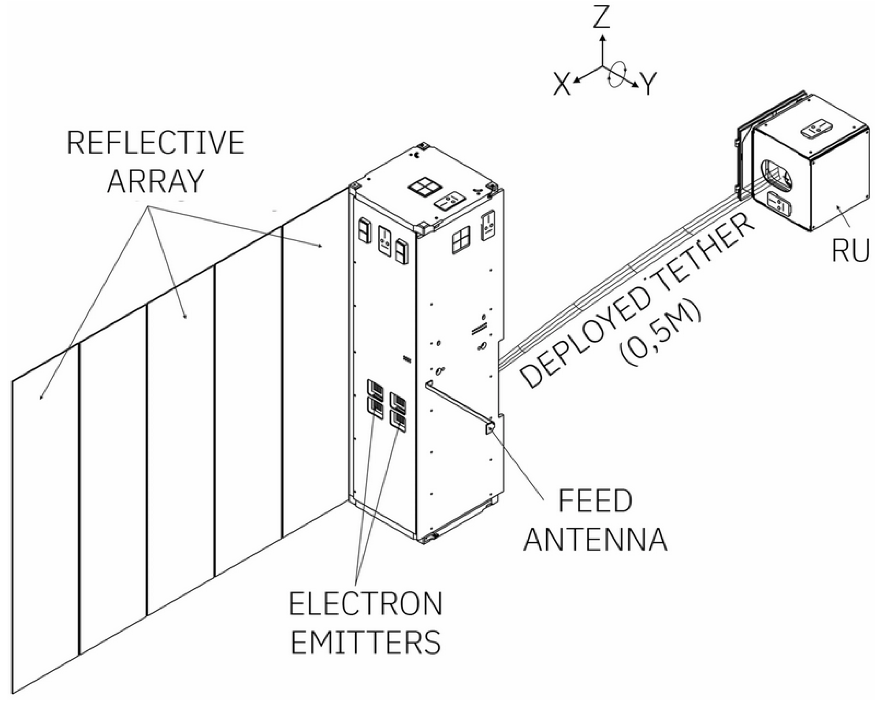
2.2. E-Sail Hardware Components

E-sail hardware consists of the following components: a tether on a motorised reel, a high-voltage source, an electron emitter, control electronics, mechanical locks, structure, enclosure and end-mass or remote unit (RU); see Figure 4 as an example of the Multi-Asteroid Touring (MAT) concept. E-sail’s early operations start with spinning up a spacecraft and deploying the tether centrifugally. The motor is used to control and measure the deployment rate. While the system’s angular momentum remains the same, the spin rate decreases as more tether is deployed. For in-orbit demonstration missions, the tether has an end mass that keeps it stretched. For more advanced E-sail missions, the end mass can be replaced by a remote unit. This results in an increase in mass and complexity, but in exchange it introduces new options, such as spin rate and plane control using an increasing arm length. Placing the spin control unit far from the spacecraft–remote unit centre of mass helps to minimise the propellant used to control the spin rate and plane orientation. When the whole tether is deployed, the E-sail can start its proper operations (more details in Section 2.3).
The tether is connected to the high-voltage source via a slip ring which ensures the electrical connection. The E-sail is operated by charging the tether and running the electron emitter. The charging can be synchronised with the spacecraft spin in order to affect the resulting thrust direction. How much to charge depends on the local solar wind conditions which are constantly monitored by measuring the tether current. In addition, tether deployment can be monitored using a camera.
The electron emitter pumps out negative charge from the spacecraft–tether system so that the tether can be maintained at a high positive potential with respect to the surrounding solar wind plasma. The emitter must produce a current which cancels the thermal electron current that the positively biased tethers gather from the plasma. The magnitude of the gathered electron current can be predicted by analytic formulas of the so-called orbital motion limited (OML) theory, initially developed in the context of Langmuir probes. We are using a cold cathode emitter which is a spin-in technology from the FEEP thruster development work [30].

2.3. E-Sail Deployment and Operations

A system consisting of several evenly spaced tethers produces a thrust vector that can be oriented by changing the spin plane alignment. This can be achieved by alternately charging the tethers in sync with the spin rate to reach a moment that will precess the spin plane. The E-sail attitude can be controlled and attitude manoeuvres are possible by tether voltage modulation synchronous with sail rotation. In particular, the sail can be inclined with respect to solar wind direction to obtain transverse thrust to change the osculating orbit angular momentum [10]. Given voltage modulation, the thrust vectoring is possible in the radial and transverse thrust vector components [11].
Our in-orbit demonstration missions thus far have a single tether and we are considering single-tether E-sail concepts in the scope of ESTCube lunar cubesat and Multi-Asteroid Touring (MAT) [29,31]. The ESTCube concept is the simplest case where the main spacecraft hosts the spin control propulsion system and there is a simple end mass keeping the tether stretched. The MAT concept, represented in Figure 5, hosts the propulsion and control system on board a remote unit that is attached to the end of the tether instead of the end mass. As the remote unit has to be a complete self-sufficient system, this solution is considerably more complex. However, having a remote unit at the end of the tether helps to minimise the spin control propellant consumption and may also improve single-tether controllability.
For the ESTCube lunar cubesat, the planned tether length is several kilometres, which requires the total angular momentum of a few 100 N ms (more trade-off details will be provided in the upcoming mission design paper). With an undeployed tether, this would require an extremely high spin rate (in the order of 1 × 10 6 deg/s) which the power production, communication and attitude control systems and the spacecraft structure would not be able to handle. This would most likely lead to a break up or a complete loss of control of the spacecraft. Therefore, the deployment must be executed in steps. The exact sizes of the steps need to be determined by a detailed analysis of the spacecraft spin dynamics.
Miniature cubesat electric propulsion thrusters will be used to spin up the spacecraft, while reaction wheels will provide precise control of the attitude and spin plane. To avoid tangling or damaging the tether, each of the spin-up steps must be carefully analysed and planned. The orbital manoeuvres, as described previously, also require spin plane control; this and other practical solutions will be presented in the upcoming ESTCube lunar nanospacecraft mission design article of the Special Issue.

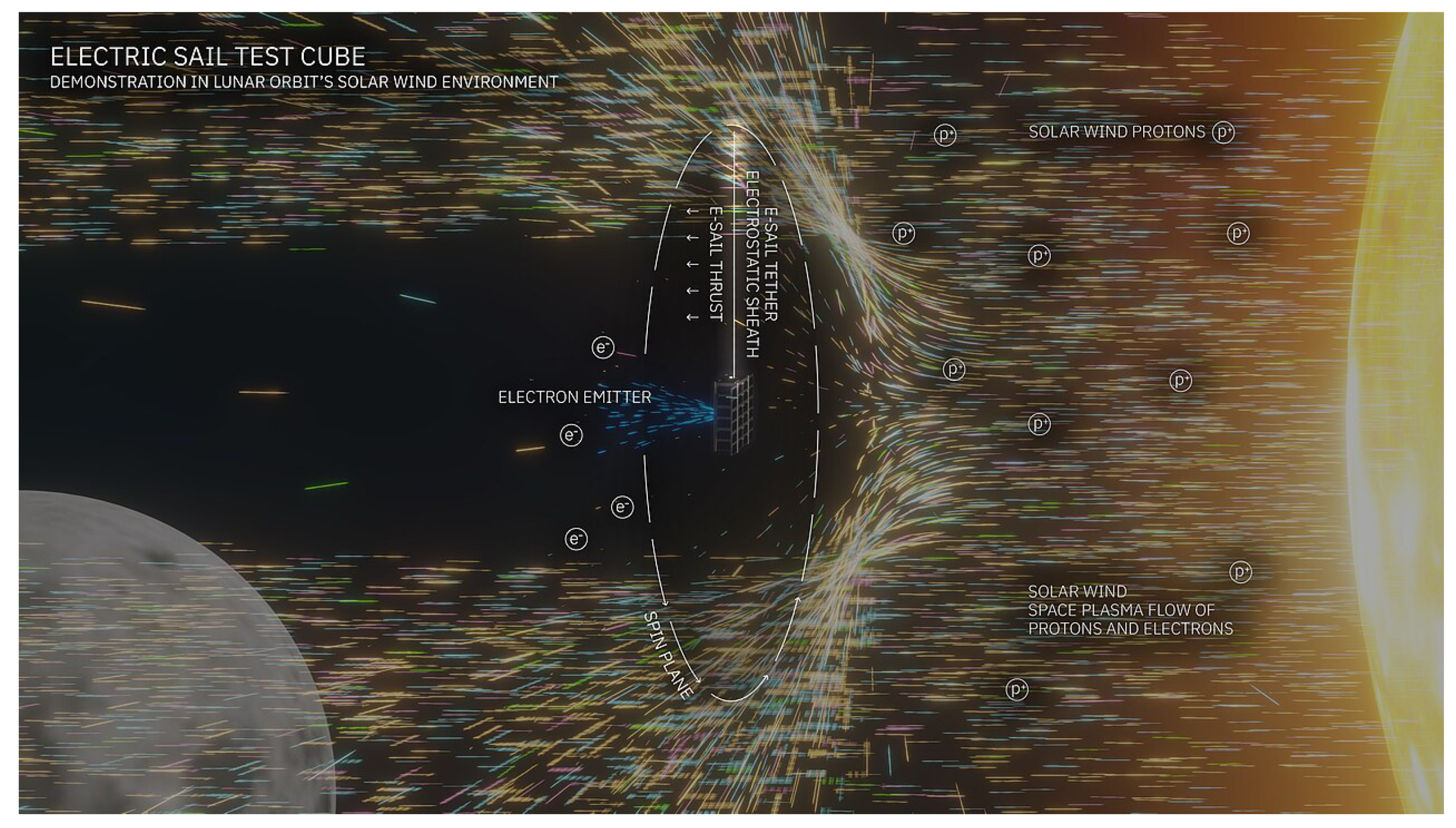
2.4. E-Sail Surrounding Space Plasma Environment

A spacecraft with a tether biased to a high positive potential interacts with the surrounding plasma in non-trivial ways. The tether reflects essentially all of the impinging ions while attracting electrons. The current balance would require the spacecraft body to become negative with respect to plasma, thus repelling the electrons and collecting more of the positive ions. However, the ion current collected by the spacecraft is not sufficient to balance the electron current collected by the tether, and an electron emitter must be used to maintain the neutrality of the platform. Yet, the interaction is by far not trivial.
A unique experiment of relevance for interaction of high-voltage positive electrodes with plasma was the Tethered Satellite System programme, with the TSS-1R experiment performed in 1996 [32]. Among the unexpected findings from the experiment were the enhanced (compared to classical theory) electron current collection by strongly positively biased surfaces, and the onset of plasma instabilities and generation of suprathermal electron and ion population when the positive potential exceeded the ram potential—that is, when the reflected ions create a counterstreaming population with the ram ions. This indicates the presence of a range of plasma physical phenomena adding extra complexity to the interaction of the tethered system. While the operation regime of the solar wind E-sail is expected to be quite different from a tethered satellite in low Earth orbit, with considerably less dense and hotter plasma and much weaker magnetic field, the general characteristics of mesosonic plasma flow suggest that some of the processes would indeed be of relevance for the E-sail conditions. To understand the interaction, it is important that the E-sail is modelled and operationally tested across a wide range of bias voltages, electron emitter currents, and ambient solar wind parameters. Additional plasma probe measurements in the vicinity of spacecraft can be instrumental in revealing some of the processes important for plasma interaction.

3. ESME: Electric Sail Mission Expeditor

The Electric Sail Mission Expeditor, or ESME, is a software package for developing and analysing Coulomb drag propulsion missions. The core functionality of the ESME is the propagation of E-sail and plasma brake orbits in varying fidelity levels, starting from Coulomb drag interaction between an E-sail tether and a space plasma flow and ending with rough-and-ready orbital propagators and trajectory browsers for a continuous expedition of the electric sail mission tradespace.
In this section, we present the initial plan of ESME development leading up to high-level functions, which will take several years to develop. Our goal is to introduce the complexity level of E-sail analysis and mission design: ESME requirements are assembled from a range of internal and public documents, such as proposals, spacecraft designs, in-orbit results and project reports. The E-sail component-level and modelling architecture in detail such as below is presented publicly in one place for the first time.
The novelty of the proposed propulsion system calls for the development of ad hoc systems for simulation and validation of its working principles, as none of the tools available for space mission design are a good fit for all the specific purposes of such a mission. Simulations of the Coulomb drag effect on tethers exist and will be used for ESME development [5,9], but their results must be expanded for the current purpose and harmonised with the rest of the ESME framework.

3.1. Software Requirements

There are several fields where the ESME needs to excel to be useful as an E-sail analysis and mission design tool. We define the initial set of ESME requirements and highlight which functions are implemented for this paper.
  • Simulate a space plasma flow on multiple scenarios:
    (a)
    on multiple solar wind regimes:
    • solar wind moving relative to the spacecraft (implemented in this paper);
    • satellite moving with respect to nearly stationary plasma in the ionosphere.
    (b)
    taking into account eclipses, magnetospheres, and solar activity;
    (c)
    with different precision levels:
    • average values for solar wind density and velocity;
    • simulated time-varying data for density and velocity;
    • user-provided datasets.
  • Simulate physical–mechanical and control models of the E-sail in multiple regimes:
    (a)
    varying levels of detail in the tether structure:
    • idealistic single-wire structure of the tether (implemented in this paper);
    • scaled effective electric radius for simulation of multi-component wires [5];
    • redundant multi-component tether [22].
    (b)
    different number of tethers per spacecraft:
    • single-tether system (implemented in this paper);
    • four-tether system;
    • generalised multi-tether system.
    (c)
    different tether deployment and E-sail control methods, accounting for changes in the moment of inertia and the centre of mass as well as propulsion required for tether deployment and navigation required for operations:
    • idealistic centrifugal tether deployment (implemented in this paper);
    • idealistic gravity gradient tether deployment;
    • realistic closed-loop electric sail deployment scheme between spin thrusters or actuators, attitude control algorithms and the tether deployment system;
    • realistic closed-loop electric sail operations and control scheme between on-board sensors, cameras, navigation and control algorithms.
  • Simulate the charging of tether, creating an electrostatic sheath that forms a virtual electric sail in negative and positive modes:
    (a)
    positive polarity for the solar wind environment which requires an electron emitter (implemented in this paper);
    (b)
    electron beam with specified current/voltage and beam divergence;
    (c)
    negative polarity for the ionospheric environment.
  • Simulate the Coulomb drag interaction between the tether and the space plasma flow—the particles are deflected creating the propulsive Coulomb drag thrust effect (implemented in this paper: one of the main E-sail experiment results presented below).
  • Calculate the E-sail trajectory by integrating classical Keplerian orbits with the Coulomb drag thrust.
  • Implement multiple orbital fidelity regimes of the E-sail:
    (a)
    Coulomb drag trajectory: represents the physical phenomena but is extremely computationally expensive; therefore, it cannot be used for full E-sail mission design (implemented in this paper);
    (b)
    Thrust per unit of tether length trajectory: physically accurate approximation which can be used to model the operations of a practical E-sail and to design high-fidelity missions;
    (c)
    Thrust vector trajectory: orbital accurate approximation which can be used to design high-fidelity orbits but does not account for the E-sail’s operational specifics;
    (d)
    Precalculated trajectory: a browser of realistic E-sail trajectories which can be used for rough-and-ready mission sketches without propagating orbits.
  • Implement an E-sail control abstraction and Application Programming Interface (API) module which would simplify the mission design process for non-experts and allow them to connect with mission and spacecraft design software that cannot model the E-sail natively:
    (a)
    Attitude and spin plane control abstraction;
    (b)
    Tether charge abstraction;
    (c)
    Trajectory output for default or user-defined abstraction parameters (i.e., how the E-sail control and charging yields the trajectory);
    (d)
    Abstraction of other control methods necessary for E-sail operations (see the proposed closed-loop control schemes above). With a future sensor implementation, the user would have an option to specify sensors and their performance or consider the E-sail as a black box that “just works” using default simplified algorithms and sensors (equivalent of the Hohmann transfer in chemical propulsion);
    (e)
    Interface with other spacecraft subsystems (could be emulated by other software or hardware tools), such as electrical power, navigation and attitude determination [33].
  • Provide the following outputs:
    (a)
    Raw data of the simulations over time where available:
    • Solar wind simulations;
    • Magnitude and direction of the generated thrust;
    • Corresponding changes in orbital parameters;
    • Changes in spacecraft attitude.
    (b)
    Graphs and plots of the results;
    (c)
    2D/3D representation of the spacecraft state, solar wind, and thrust;
    (d)
    Graphical representation of the orbital trajectory.

3.2. Initial Architecture

An overview of the planned software architecture for the ESME can be seen in Figure 6. It shows that the input data provided by the user is sent to all the necessary simulations in order to output the trajectory of the spacecraft after the Coulomb drag interaction along with all the raw data of the intermediate steps.
The input from the user of the ESME will be gathered through a graphical user interface (GUI, for short). It will require details about the spacecraft, its position and velocity in the Solar System or low Earth orbit, and the relative orientation between the spinning plane of the tether and the wind. As new values become added, the graphical representation of the spacecraft and its environment will be updated.
The ESME requires certain information about the spacecraft, namely the body mass and the tether material density, the number of tethers, their structure (if they have end masses or remote units and how the tether is deployed), the maximum length, etc.
The position and velocity of the spacecraft are required to calculate the unpowered orbit to be compared with the resulting orbit after the Coulomb interaction takes place. Initially, the system of reference for these variables corresponds to the lunar mission that the ESME is being built to support, meaning a geocentric or lunar-centric system of coordinates. However, multiple reference systems should be included in the future, and the user should be allowed to decide.
The position of the spacecraft in the solar system can also be used to determine the normal conditions of the solar wind at that distance from its source, although the user can overrule the calculation and input a different density and charge of the wind in order to simulate scenarios like exceptional solar weather events or the environment around a different star.
After all the data is introduced, several simulations can take place. Firstly, a physical model of a tether is created. It must be able to simulate a tether divided into several sections that can each be affected by the Coulomb drag and the centrifugal forces with different intensities, but constrained into a tether shape with the stiffness corresponding to the material. The resolution of the tether model can be adjusted in order to change the balance between good spatial resolution and fast performance, allowing even to use extra resolution for specific phases, like the unreeling process, for example.
Alongside the physical model of the tether, the charging process must be simulated. The electrical repulsion between charged tethers affects their shape, which affects the charging process in a feedback loop that can complicate the simulation development. Luckily, the effect is negligible, and it can be safely ignored. Both positive and negative modes are to be represented, up to the maximum voltages expected for propulsion purposes. The end result is a distribution of charges along the length of the tether and the resulting fields around it.
The combination of the physical model of the tether, its charge, and the conditions of the solar wind environment are fed into the Coulomb drag simulation. It reproduces the interaction between the charges in the wind and in the tether, producing reaction forces and a redistribution of the surface charges. The redistribution of charges eventually negates the voltage on the tether unless compensated by an electron emitter or by the ionosphere of the Earth, so the Coulomb drag and charging simulations depend on each other when simulating for periods of time.
Once the results of the Coulomb interaction are known, the total thrust produced by the system at a given point in time can be calculated. If the spacecraft has multiple deployed tethers, the ESME takes them all into account and adds up their effects. At this stage, some extra phenomena must be considered, like the slight delay of the E-sail thrust when a tether is charged, as some energy is used by the deformation of the tethers into their equilibrium shape, or how sudden changes in the solar wind conditions can also cause oscillations in the tether shape. Active charge modulation on individual tethers can solve the oscillation problems [34].
Different tethers must be capable of being charged at different voltage levels for attitude control purposes. Spacecraft orientation with respect to the wind direction plays a role in the calculation because the thrust is generated in the perpendicular direction to the spinning plane, and the orientation of the plane can be purposefully modified in order to induce changes in the orbit.
The orbit propagator will be the final step of the pipeline. Using the spacecraft position and velocity in the given system of reference, the expected free-flying trajectory will be computed, and by adding the thrust provided by the sail during the manoeuvre, the new trajectory will be obtained. This will not only allow the user to plan specific orbital manoeuvres, but also provide information on the expected effects of the E-sail, which will be useful for the validation of the sail on its first missions.
The end results from the ESME consist of the data from all the simulations involved: Coulomb drag interaction between the tether and solar wind, thrust expected for the spacecraft under study, and the expected changes in its orbital path. Even though the results will be presented to the user as plots, the raw data will always be available for external analysis.
As presented above, the ESME will provide mission design functionality for engineers and scientists with a background on the fundamentals of E-sail propulsion. The multiple pieces that compose the ESME, shown in Figure 6, comprise a full simulation of the behaviour of a E-sail propelled spacecraft which can be used for all phases of the mission planning, development, and operations. A spacecraft with any number of tethers, with any choice of length and voltage, and for any solar weather conditions, can be modelled with ease, and all the necessary data will be available as output. Once an orbit propagator is integrated into the ESME or developed from scratch, the effect of the E-sail will be reflected in its orbital changes, extending the functionality of the ESME to orbit planning and numerical trajectory design. Integration with known mission analysis tools like STK or GMAT will be available as well, for users who prefer to use those tools for overall mission design.

3.3. Current State of Development

At the time of publication, the basic building blocks of the ESME have been developed. The system can receive user input from the mouse and keyboard, and it outputs real-time graphical output in 3D. Some variables can be changed from the GUI using sliders or input boxes; the rest are only accessible from code for now.
Cubesat body, E-sail elements, and end mass are represented, both graphically (Figure 7) and as physical entities in the simulation. The solar wind is present as a vector with a given velocity, but has no graphical representation for now.
The E-sail is simulated as a series of individual points that are subjected to forces independently of each other. The total length of the tether and the density of points per meter can be changed by the user through modification of the code. The simulation of the effect of the forces on the E-sail elements is performed using the Verlet integration without velocities. In order to keep the elements from drifting apart, a distance constraint is applied iteratively to all elements of the E-sail, right after the Verlet integration has been performed.
The E-sail can be deployed by the user, element by element, and charged positively or negatively. Once an element is deployed, it suffers and reacts to the centrifugal force and, if the E-sail is charged, to a Coulomb drag force in the direction of the solar wind.
The resulting force of the interaction between the charged E-sail segments and the solar wind is compatible with the results in [5]. The simulation must be updated to the new iterative method shown in [8].
ESME is available as an open source (https://github.com/marioferpa/ESME, accessed on 11 June 2023).

4. ESME Development Toolkit

We developed the initial functions of the ESME from scratch, which allowed us to consider the fundamental computer science questions in how a modern scientific modelling tool could be developed. This section introduces the notable features of the ESME in terms of the programming language and paradigm, GUI, the modelling of physics and the treatment of physical units.

4.1. The Rust Programming Language

The ESME is being written in the Rust programming language [35]. It is a compiled language designed, from the ground up, to have good performance, memory safety, and simple access to parallel computing—characteristics that are very welcome for a realistic simulator. It provides access to low-level programming methods, along with high-level programming, building on the legacy of other older, bulkier languages like C++.
It is rapidly rising in popularity, meaning that more libraries (called crates in Rust) and resources are being added to its ecosystem every year, and that a very large and active community is available for solving problems.
Several crates are being developed in the field of simulation, like Rapier for physics simulations and Salva for fluid simulations. As they market themselves as good resources for programming physics for video games, which could mean that they sacrifice realism in exchange for real-time results, the crates results will have to be validated, and custom tools be created where necessary. There are also multiple crates available for algebra and numerical analysis (nalgebra and Peroxide, for example), and for Finite Element Analysis (like Fenris). In the case of the ESME, all physics-related computations are being developed from the ground up.
Rust also has a Foreign Function Interface (FFI) that makes it capable to load and use functions written in the C programming language, expanding its toolset even more. It is technically possible to use C++ functions as well, although this is not natively supported and must be performed using external crates.

4.2. Strategic Use of a Game Engine

Some aspects of the ESME are being developed using an open-source game engine called Bevy [36] written in Rust. The benefit of using such a tool for the ESME is that there is some overlap between a scientific simulation with good user input and graphical output and a video game, and therefore, many of the tools that have been developed for gaming can be useful for scientific visualisation, GUI and software architecture. Although it is possible to gather the tools necessary for every need of the simulation one by one, it can be more convenient to obtain a video game engine and simply pick what is useful and leave out what is not, especially those parts that could interfere with the scientific results.
The main features from Bevy that are being used in the ESME are:
  • User interface (Text boxes, Sliders, Camera control with mouse).
  • Graphical output (3D graphics, Camera, Illumination).
  • Entity–Component–System architecture, detailed below.
However, there are some aspects in which the goals of scientists and game designers stop overlapping. In particular, game engines stop being useful when any physics-related calculation is required. Game designers do not usually need to perform realistic simulations, but rather simulations that look realistic enough while also running in real time in a specific device, sometimes leading to quantitatively and qualitatively different results depending on the hardware performance. They usually choose performance over realism and perform several tricks and approximations behind the scenes that would make the results inviable for science. For this reason, the code for the Coulomb drag interaction, and every other physical simulation, is being written from scratch.

4.3. Entity–Component–System

Entity–Component–System (ECS) is a software architecture pattern that is seen as an improvement over the more widely known Object-oriented programming (OOP) paradigm. The fundamental structural element of OOP is the concept of the class, a template that encapsulates both data and behaviour. Objects can be created from those classes and be used to represent all the physical elements that need to be modelled in the simulation. In order to avoid repetition of code when multiple classes share similar functionality, the concept of inheritance can be used, in which a class inherits all the properties and functions from a parent class and adds new properties, or overwrites some properties in order to better suit its needs.
A common pitfall with OOP programming is that inheritance trees can become very deep and complex, making improvement and maintenance really complicated. A change in parent class can have cascading effects that require lots of extra work, and the abstraction that was helpful at first can quickly become an obstacle.
ECS was born in the video game world, but it seems as a convenient evolution from OOP for every purpose. In this architecture, there are three distinct components:
  • Entities: An Entity can be created for every distinct element that is present in the simulation. Internally, an Entity is nothing more than an ID number that uniquely identifies it among all other entities in existence.
  • Components: Components are reusable pieces of code that model specific behaviours for the Entities. Ideally, they only contain data, plus methods for modifying said data.
  • Systems: Systems are functions that operate at run time, gathering the Entities that have specific sets of Components, and act on them.
A beneficial side effect of ECS is that parallel computing becomes very accessible. If two systems try to run in the same time step and do not require mutable access to the same entities, they can be run in parallel.
Systems can add or remove components from entities at run time. For example, a voltage component can be added or removed depending on the situation. This further separates this method from OOP, where class contents can not be modified while the system is running.

4.4. UOM (Units of Measurement) Package

The ESME is being built from the start with dimensional analysis in mind, specifically with the use of the uom crate [37]. What this means is that every physical unit that is managed in the code is not saved as a numerical type without units, but as a type corresponding to the physical unit in question that keeps track of the units. Variables are created specifying the type, the magnitude, and the unit, and they are saved internally as the base unit of the International System of units regardless of the original input. Operations between uom types are automatically performed in the base unit, preventing conversion errors or inputs in different systems of units to alter important results. If a dimensionally incorrect operation is attempted, an error is raised.
The inclusion of a dimensional analysis package increases code complexity, but totally prevents the possibility of human errors in regard to units from affecting the result. Also, it plays well with the philosophy of the Rust programming language of preventing the user from writing unsafe code and catching errors at compile time instead of at run time: if a dimensionally incorrect operation will be performed, compilation will be halted.

5. E-Sail Experiment Design for Lunar Orbit

As the initial case study of the ESME, we consider an E-sail demonstration mission. Two main scenarios have been considered for the mission: a highly elliptical orbit (HEO) around the Earth and a lunar orbit. Table 1 summarises the most important mission aspects of GTO versus the lunar orbit in terms of characterising the Coulomb drag effect and demonstrating the E-sail technology.

5.1. Highly Elliptical Orbit

A highly elliptical orbit (HEO) would be easier to reach from Earth than a lunar orbit: for example, launches to geostationary transfer orbit (GTO) are common; therefore, a small mission could share a rocket with a satellite travelling to the geostationary orbit, and later rise its apogee to the required 30 Earth radii. Moreover, it would provide opportunities to test the Coulomb drag effect in varying plasma densities ranging from the ionosphere near the perigee to the radiation belt. The Foresail-2 mission is designed to characterise the Coulomb drag effect and to study the radiation belt with cubesats.
The major challenge of a HEO mission is that the satellite would have to cross the Van Allen belt twice per round, posing a threat to its electronic components and requiring novel cubesat-compatible radiation hardening solutions. Compared with the LEO missions, new operational and communication solutions are necessary in order to accommodate the constantly changing environmental and orbital parameters. For example, the plasma densities differ by orders of magnitude between the perigee and the apogee and so do orbital parameters as the satellite changes its altitude from hundreds to tens of thousands of kilometers. These changes require the Coulomb drag experiment to run in harmony with the attitude and orbit determination system while also finding a suitable orientation for data downlink.
Another challenge is that the orbital plane maintains its orientation during Earth’s travel around the Sun. This means that it is not possible to choose the apsides to be in beneficial positions during the whole year, with an alignment between solar wind direction and orbital velocity in the apogee, for example, or one that minimises the time spent in eclipse.

5.2. Lunar Orbit

A lunar orbit would provide the spacecraft with frequent access to undisturbed solar wind, excellent conditions for demonstrating the E-sail. The spacecraft would spend about two thirds of the mission lifetime in the solar wind and about one third in the lunar wake and in the Earth’s magnetosphere which blocks the solar wind. The solar wind would be blocked when the Moon crosses the Earth’s magnetotail (about a fourth of its orbital period [38]), and when the spacecraft is eclipsed behind the Moon. In the latter situation, the E-sail experiment would not be performed in any case, as there is no access to solar power. In total, the spacecraft would have access to solar wind for two thirds of the time, sufficient for its purposes.
An important fact to consider is that lunar orbits decay very rapidly due to tidal interactions and the mass concentrations (or mascons) present on the Moon. Lunar mascons affect lunar orbits under 750 km, and for orbits of 100 km or less, their effect dominates so much that third-body interactions can be neglected [39]. Orbits affected by mascons suffer from eccentricity and argument of periapsis drift, and soon intersect with the lunar surface.
Although the mission will probably not proceed to a low lunar orbit where mascon influence is greatest, it could be helpful to avoid their interference as much as possible, considering that the more stable the orbit, the better the extracted effect of the solar sail on propulsion. For this purpose, it could be interesting to launch into a so-called frozen orbit, at an inclination of 27°, 50°, 76°, or 86° [39]. Again, this depends on the rocket launchers available, or on the capabilities of the vehicle that will be used for orbit insertion.
Assuming a suitable lunar launch, we consider the communications and operations to be less complex than in the HEO case, although a large parabolic antenna is necessary to communicate with the spacecraft.
In order to fulfil the goal of designing an E-sail demonstration mission, we are proceeding with the lunar orbit case. As shown in Figure 8 on E-sail experiment design, the lunar orbit provides pristine E-sail measurement conditions in the solar wind for roughly two thirds of the mission time, a good compromise for a mission in the cis-lunar environment. Moreover, the FORESAIL consortium is already designing a mission for the HEO scenario.

6. ESTCube Lunar Nanospacecraft E-Sail Experiment Simulation

The first objective was to verify the results from Janhunen et al. [5]. They show that a small sat of 287 kg, carrying 100 radial tethers of 21 km in length each, accelerating out of the solar system from 1 AU would accelerate at 4.2 mm/s 2 and reach a final velocity of 82 km/s. This setup is very different from that of the first lunar mission presented in this paper, with a 6 U cubesat of 15 kg deploying a tether of approximately 1 km. However, the force per unit length simulated by the ESME is compatible with these results, giving the cubesat an estimated acceleration of 5.01 × 10 6 ms−2.
Table 2 shows the resulting force for different combinations of charging voltage and tether length, simulated by ESME. The calculation considers a solar wind density of 7.3 cm−3 and a velocity of 4.0 × 10 5 ms−1.

7. ESTCube Lunar CubeSat Orbit Escape Control Law and Trajectory Design

7.1. E-Sail Orbital Dynamics

To illustrate the E-sail orbital dynamics, consider an ESTCube lunar cubesat escape mission scenario, which is consistent with the E-sail experiment design in lunar orbit illustrated in Section 5. In this context, the spacecraft is modelled as a point mass in a selenocentric orbit, subject to the Moon’s gravitational force, the E-sail thrust, the Earth’s (third-body) gravitational attraction, and the perturbative force due to the Moon’s oblateness. The perturbation caused by the Sun’s gravitational attraction can be neglected within the lunar sphere of influence, as it is at least two orders of magnitude smaller than that of the Earth.
The spacecraft equations of motion have been numerically integrated using a classical built-in MATLAB routine and, to facilitate the inclusion of Earth, Moon, and Sun ephemerides, which are typically expressed in the International Celestial Reference Frame (ICRF), the equations of motion are formulated in a Moon-centred reference frame T ( O ; x , y , z ) whose axes are parallel to the ICRF ones. In particular, the x axis is directed towards the Aries point ⥾, the z axis points towards the Celestial North Pole, and the principal plane ( x , y ) coincides with the true celestial equator. The perturbative acceleration due to the Earth’s gravitational attraction is expressed as
a = μ r S r S 3 r r 3 ,
where μ 3.986 × 10 5 km 3 /s 2 is Earth’s gravitational parameter, r S is the Earth–spacecraft vector, and r is the Moon–Earth vector. The perturbative acceleration vector a J 2 due to the Moon’s oblateness has been calculated considering only the influence of the second zonal harmonic J 2 = 202.43 × 10 6 . In particular, vector a J 2 can be conveniently expressed in a reference frame T ( O ; x , y , z ) , with origin O at the Moon’s center of mass and unit vectors { i ^ , j ^ , k ^ } , where the x axis is directed towards ⥾, the z axis is aligned with the Moon’s North Pole, and the principal plane ( x , y ) coincides with the lunar equatorial plane. Reference frame T can be obtained by rotating reference frame T around the x-axis by an angle of γ = 21.92 deg; see Figure 9.
The perturbative acceleration caused by the lunar J 2 can be expressed in T as
a J 2 T = U J 2 = U J 2 r [ i ^ R ] T + U J 2 z [ k ^ ] T ,
where i ^ R is the radial outward unit vector, r is the distance of the spacecraft from the Moon’s center of mass, and U J 2 is the perturbative part of the gravitational potential caused by J 2 . The partial derivatives appearing in the equation are
U J 2 r = μ J 2 R 2 r 4 3 2 15 2 z 2 r 2 , U J 2 z = 3 μ r 5 J 2 z R 2 ,
where μ = 4.902 × 10 3 km 3 / s 2 is the Moon’s gravitational parameter, and R = 1737.4 km is the Moon’s mean equatorial radius. The perturbative acceleration a J 2 , obtained through Equations (6) and (7), can be expressed in T as
a J 2 T = T γ · a J 2 T ,
where
T γ = 1 0 0 0 cos γ sin γ 0 sin γ cos γ .
Accordingly, the spacecraft equations of motion are
{ r ˙ = v v ˙ = μ r 3 r a + a J 2 + a T ,
where r = [ x , y , z ] T (or v = [ v x , v y , v z ] T ) is the spacecraft position (or velocity) vector. The spacecraft equations of motion can be rewritten in a dimensionless form by introducing the Distance Unit ( D U = R ) and the Time Unit ( T U = D U 3 / μ 1034.3 s) so that one has
r ˜ = r D U v ˜ = v T U D U a ˜ = a T U 2 D U a ˜ J 2 = a J 2 T U 2 D U a ˜ T = a T T U 2 D U μ ˜ = μ T U 2 D U 3 .
The dimensionless equations of motion are therefore
{ r ˜ ˙ = v ˜ v ˜ ˙ = μ ˜ r 3 r ˜ a ˜ + a ˜ J 2 + a ˜ T .

7.2. Orbit Escape Control Law and Trajectory Design

Consider an orbital (right-handed) reference frame T O ( S ; x O , y O , z O ) with unit vectors { i ^ r , i ^ t , i ^ n } in which the x O axis is directed along the outward radial direction and the z O axis is aligned with the spacecraft angular momentum vector. The sail orientation is defined by the two control angles, η [ 0 , π ) rad and ξ [ 0 , 2 π ) rad, where η is the angle between the direction of a T and that of i ^ n , and ξ is measured counterclockwise from i ^ t to the projection of a T on the orbital plane ( i ^ r , i ^ t ) ; see Figure 10. Note that τ is the third control parameter in the E-sail-based trajectory design [41,42].
The spacecraft uses a locally optimal control law aimed at instantly maximising a linear combination of the time derivatives of osculating orbit semi-major axis a and eccentricity e. The approach is consistent with the method proposed in the recent literature [43] to achieve the escape condition, which corresponds to an osculating orbit with zero specific mechanical energy [44,45].
In particular, that linear combination must allow a fast escape manoeuvre while avoiding excessive reduction in the orbit pericenter radius r p , which could lead to an impact on the lunar surface. Instead of minimising a functional given by a linear combination of the orbital parameters, the propulsive acceleration direction that maximises the value of a ˙ and e ˙ , without taking into account perturbative accelerations, is analytically computed so that the computational time is significatively reduced when compared with a (complete) numerical approach. Consequently, the optimal direction of the propulsive acceleration vector is obtained in a closed form. Finally, the values of the two control angles { η , ξ } are obtained by maximising the component of the propulsive acceleration vector a ˜ T along the desired direction.
Bearing in mind Equation (3), it can be verified that the direction of the spin axis (i.e., the direction of the unit vector k ^ B ) that maximises the projection of the thrust vector along a given direction w ^ coincides with the bisector of the unit vectors r ^ and w ^ . The directions of the propulsive acceleration that maximise a ˙ and e ˙ are, respectively, the velocity unit vector v ^ and k ^ e , which is given by
k ^ e = 4 μ / r 2 v 2 r · v r ^ + 4 v 2 r 2 4 r μ 2 r · v 2 v ^ 4 μ / r 2 v 2 r · v r ^ + 4 v 2 r 2 4 r μ 2 r · v 2 v ^ .
The time derivative of the pericenter radius,
r ˙ p = a ˙ ( 1 e ) e a ˙ ,
can be maximised by aligning the propulsive acceleration vector along unit vector k ^ p defined as
k ^ p = 4 μ / r 2 v 2 r · v r ^ + 4 v 2 r 2 4 r μ 2 r · v 2 4 μ 1 e e a v ^ 4 μ / r 2 v 2 r · v r ^ + 4 v 2 r 2 4 r μ 2 r · v 2 4 μ 1 e e a v ^ .
Accordingly, the locally optimal control law can be summarised as follows: if pericenter radius r p of the osculating orbit is below a given threshold value r p min , k ^ B is oriented to maximise the acceleration projection along k ^ p and avoid collision; otherwise, unit vector k ^ B is oriented to maximise the projection of the propulsive acceleration along k ^ e in order to achieve escape conditions as rapidly as possible. This specific strategy is chosen after observing that maximising e ˙ provides a faster escape strategy compared to maximising a ˙ or linear combinations of a ˙ and e ˙ . However, such strategy also increased the risk of impact with the lunar surface. Finally, the switching parameter control law is selected as follows: the E-sail charge is turned off (i.e., τ = 0 ) when the spacecraft is in eclipse conditions, or the Moon passes through the Earth’s magnetosphere, or the projection of the propulsive acceleration along k ^ p (or v ^ ) is negative.
Indeed, when the spacecraft is in eclipse conditions, the solar wind is shielded by the Moon and cannot reach the E-sail. In this case, a cylindrical shadow model has been considered; therefore, the condition that corresponds to the spacecraft being in the Moon’s shadow is
r ^ · r ˜ > 0 r ˜ r ^ · r ˜ r ^ < 1 D U ,
where r ^ is the Sun–Moon unit vector.
On the other hand, when the Moon passes through the Earth’s magnetosphere, it is preferable to turn off the E-sail charge because the solar wind is shielded by the Earth’s magnetosphere. In this case, the Earth’s magnetosphere has been approximated as a cylinder extending in the anti-Sunward direction from the Earth, in which the Moon spends about a quarter of its orbital period. That sort of right circular cylinder has a radius R mag of approximately 30 Earth’s radii [46], so that the condition that corresponds to spacecraft being in the magnetosphere can be expressed as
r ˜ · r ^ > 0 r ˜ r ˜ · r ^ r ^ < R ˜ mag ,
where r ˜ is the dimensionless Earth–Moon position vector, r ^ is the Sun–Earth unit vector, and
R ˜ mag = R mag D U
is the dimensionless version of R mag .
Finally, τ = 0 when the projection of the propulsive acceleration of the E-sail along the direction of k ^ p (or the direction of v ^ ) is negative because (i) in the first case, there would be an undesired reduction in the pericenter radius, (ii) in the second case, there would be a reduction in the semi-major axis, which would hinder the spacecraft from reaching an escape condition.

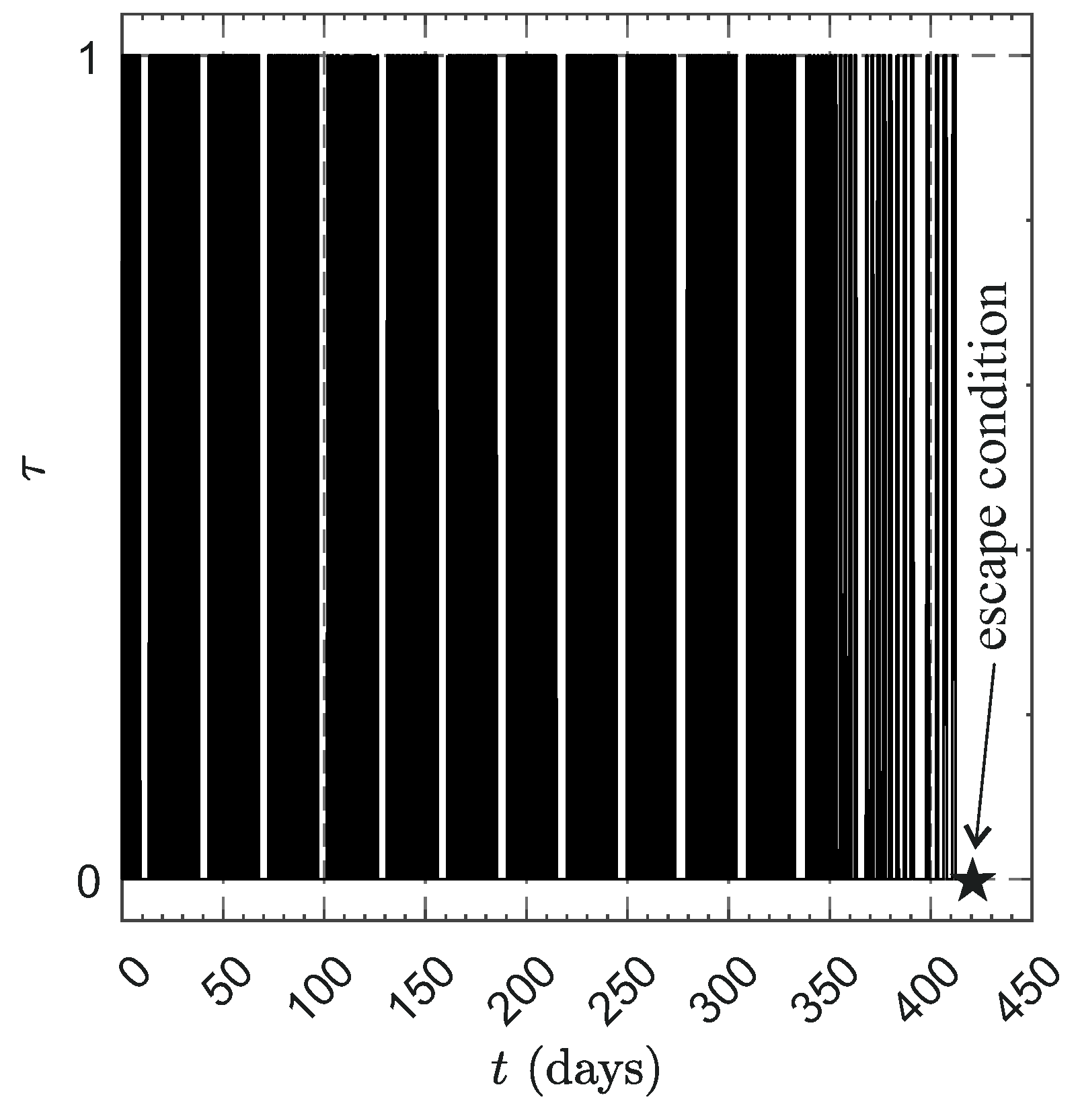
7.3. Numerical Results

This section presents simulation results for a set of representative cases, exploring variations in both initial conditions and tether characteristics. In particular, the simulations focused on circular selenocentric parking orbits along the lunar equatorial plane with initial altitude h { 100 , 500 , 1000 } km and a spacecraft mass of 15 kg. The tether voltage was set at V = 20 kV while different tether lengths were considered, that is, L { 1 , 2 , 4 } km. The minimum threshold value of the pericenter radius was set to three times the lunar mean radius (i.e., r p min = 3 DU), and the manoeuvre’s starting date was 1 January 2028. The results are summarised in Table 3, including the characteristic acceleration values, denoted as a c , representing the maximum magnitude of the propulsive acceleration vector when the Sun’s distance is one astronomical unit, viz.,
a c = σ u L m .
In the case of the parking orbit with an initial altitude of 1000 km and a tether of 4 km, the E-sail charge is turned on for approximately 26.6% of the total flight time. In this case, the time variation of the switching parameter τ is illustrated in Figure 11, which shows the low-frequency changes attributed to the influence of the Earth’s magnetosphere. On the other hand, the high-frequency variations are a consequence of the other control law constraints, and exhibit a period equal to that of the osculating orbit. As expected, this period increases during the maneuver. Examining the graph sketched in Figure 12, it is evident that the spacecraft’s average altitude gradually rises over time, as expected. The black star represents the point in which the spacecraft reaches the escape conditions. Finally, the three-dimensional escape trajectory is reported in Figure 13.

8. Conclusions

This paper shows the first steps towards the creation of the ESME—the Electric Sail Mission Expeditor, the much needed simulation suite for E-sail mission planning. The specifics of the possible E-sail missions in the near future have been laid out, and from them, the requirements for the ESME have been inferred. Two types of simulations are presented: the solar wind experiment to demonstrate the E-sail acceleration and the trajectory experiment in the lunar orbit to demonstrate the E-sail propulsion in escaping the lunar orbit. This paper is bridging the gap between computationally expensive numerical simulations and computationally lightweight analytical solutions which are solved and optimised numerically. For the first time, we have presented both solutions side by side in order to take the next steps in ESTCube lunar nanospacecraft mission design and in numerical propagation of E-sail orbits. The ESTCube lunar nanospacecraft concept will be published subsequently in Special Issue “Advances in CubeSat Sails and Tethers”. The next step in the ESME development is integration with an orbit propagator for which the minuscule E-sail force can be added as a perturbation on a classical trajectory.
We have gathered the necessary literature, set the requirements and provided a novel case study of demonstrating the electric sail in the solar wind. The development of the ESME is underway, following the planned structure, and its most basic components are already built or are in the process of being finished. Basic Coulomb drag calculations are being performed in the elements of the E-sail and are compatible with the original simulation results. The development will continue from here until all the requirements listed in this paper have been met. The simulation of the Coulomb drag combined with an orbit propagator can turn the ESME into a complete trajectory analysis tool for E-sail missions. With the planned improvements on the simulation of the tether, the value of the Coulomb drag for multiple geometries and situations will be available; the ESME has the potential to be the main mission design tool of the future E-sail lunar cubesat and other missions.

Author Contributions

Conceptualisation: M.F.P., P.J., G.M., A.A.Q. and A.S.; methodology: M.F.P., P.J., P.T., M.T., I.I., A.M., N.O., J.K., A.R., J.D., H.T., K.A., M.P., L.N., M.B., G.M., A.A.Q., N.I., J.S., A.V., A.T. and A.S.; software: M.F.P., A.M. and N.O.; validation: M.F.P., P.J., P.T., M.T., I.I., A.M., N.O., J.K., A.R., J.D., H.T., K.A., M.P., L.N., M.B., G.M., A.A.Q., N.I., J.S., A.V., A.T. and A.S.; investigation: M.F.P., P.J., A.M., N.O., G.M., A.A.Q. and A.S.; data curation: M.F.P., A.M. and N.O.; writing—original draft preparation, M.F.P., A.M., N.O. and A.S.; writing—review and editing: M.F.P., P.J., I.I., J.D., J.K., A.A.Q., N.I. and A.S.; visualisation: M.F.P. and artists referenced in captions; supervision: P.J., G.M. and A.A.Q.; project administration: A.S. and A.R.; funding acquisition: M.F.P., P.J., M.P., G.M., A.A.Q., N.I., A.V., A.T. and A.S. All authors have read and agreed to the published version of the manuscript.

Funding

The Tartu Observatory, the University of Tartu, the European Regional Development Fund supported the research and development for this article. The European Union supports the ESTCube-2 launch in LEO on board Arianespace’s Vega-C rocket in cooperation with the European Space Agency via the In-Orbit Demonstration and Validation (IOD/IOV) initiative.

Data Availability Statement

The ESME is available as an open source at https://github.com/marioferpa/ESME (accessed on 11 June 2023), under MIT license.

Acknowledgments

We thank the hundreds of people who have supported the Electric Sail Test Cube Programme since 2008.

Conflicts of Interest

The authors declare no conflict of interest.

Abbreviations

The following abbreviations are used in this manuscript:
AUAstronomical Unit
ECSEntity–Component–System
ESTCubeElectric Solar Sail Test Cube
ESMEElectric Sail Mission Expeditor
GTOGeostationary Transfer Orbit
GUIGraphical User Interface
HEOHighly Elliptical Orbit
LEOLow Earth Orbit
OOPObject-oriented Programming
PICParticle-in-cell
SISPOSpace Imaging Simulator for Proximity Operations

References

  1. Electric Sailing. Papers, Press Releases and Workshop Material. Available online: https://www.electric-sailing.fi/publications.html (accessed on 11 June 2023).
  2. Hoyt, R.P.; Forward, R.L. Alternate Interconnection Hoytether Failure Resistant Multiline Tether. U.S. Patent No. 6,286,788, 11 September 2001. [Google Scholar]
  3. Electric Solar Wind Sail. Available online: https://space-travel.blog/esail542-4028fa60700e (accessed on 11 June 2023).
  4. Bassetto, M.; Niccolai, L.; Quarta, A.; Mengali, G. A comprehensive review of Electric Solar Wind Sail concept and its applications. Prog. Aerosp. Sci. 2022, 128, 100768. [Google Scholar] [CrossRef]
  5. Janhunen, P.; Sandroos, A. Simulation study of solar wind push on a charged wire: Basis of solar wind electric sail propulsion. Ann. Geophys. 2007, 25, 755–767. [Google Scholar] [CrossRef] [Green Version]
  6. Janhunen, P. Electric Sail for Spacecraft Propulsion. AIAA J. Propuls. Power 2004, 20, 763–764. [Google Scholar] [CrossRef]
  7. Janhunen, P. On the feasibility of a negative polarity electric sail. Ann. Geophys. 2009, 27, 1439–1447. [Google Scholar] [CrossRef] [Green Version]
  8. Janhunen, P.; Toivanen, P.K.; Polkko, J.; Merikallio, S.; Salminen, P.; Haeggström, E.; Seppänen, H.; Kurppa, R.; Ukkonen, J.; Kiprich, S.; et al. Invited Article: Electric solar wind sail: Toward test missions. Rev. Sci. Instrum. 2010, 81, 111301. [Google Scholar] [CrossRef]
  9. Janhunen, P. Simulation study of the plasma-brake effect. Ann. Geophys. 2014, 32, 1207–1216. [Google Scholar] [CrossRef] [Green Version]
  10. Toivanen, P.; Janhunen, P.; Envall, J. Electric sail control mode for amplified transverse thrust. Acta Astronaut. 2015, 106, 111–119. [Google Scholar] [CrossRef] [Green Version]
  11. Toivanen, P.; Janhunen, P. Thrust vectoring of an electric solar wind sail with a realistic sail shape. Acta Astronaut. 2017, 131, 145–151. [Google Scholar] [CrossRef] [Green Version]
  12. Envall, J.; Janhunen, P.; Toivanen, P.; Pajusalu, M.; Ilbis, E.; Kalde, J.; Averin, M.; Kuuste, H.; Laizans, K.; Allik, V.; et al. E-sail test payload of ESTCube-1 nanosatellite. arXiv 2014, arXiv:1404.6961. [Google Scholar] [CrossRef]
  13. Praks, J.; Mughal, M.R.; Vainio, R.; Janhunen, P.; Envall, J.; Oleynik, P.; Näsilä, A.; Leppinen, H.; Niemelä, P.; Slavinskis, A.; et al. Aalto-1, multi-payload CubeSat: Design, integration and launch. Acta Astronaut. 2021, 187, 370–383. [Google Scholar] [CrossRef]
  14. Seppänen, H.; Rauhala, T.; Kiprich, S.; Ukkonen, J.; Simonsson, M.; Kurppa, R.; Janhunen, P.; Hæggström, E. One kilometer (1 km) electric solar wind sail tether produced automatically. Rev. Sci. Instrum. 2013, 84, 095102. [Google Scholar] [CrossRef] [PubMed]
  15. Slavinskis, A.; Pajusalu, M.; Kuuste, H.; Ilbis, E.; Eenmäe, T.; Sünter, I.; Laizans, K.; Ehrpais, H.; Liias, P.; Kulu, E.; et al. ESTCube-1 In-Orbit Experience and Lessons Learned. IEEE Aerosp. Electron. Syst. Mag. 2015, 30, 12–22. [Google Scholar] [CrossRef]
  16. Mughal, M.R.; Praks, J.; Vainio, R.; Janhunen, P.; Envall, J.; Näsilä, A.; Oleynik, P.; Niemelä, P.; Nyman, S.; Slavinskis, A.; et al. Aalto-1, multi-payload CubeSat: In-orbit results and lessons learned. Acta Astronaut. 2021, 187, 557–568. [Google Scholar] [CrossRef]
  17. Dalbins, J.; Allaje, K.; Iakubivskyi, I.; Kivastik, J.; Komarovskis, R.O.; Plans, M.; Sünter, I.; Teras, H.; Ehrpais, H.; Ilbis, E.; et al. ESTCube-2: The Experience of Developing a Highly Integrated CubeSat Platform. In Proceedings of the 2022 IEEE Aerospace Conference (AERO), Big Sky, MT, USA, 5–12 March 2022; pp. 1–16. [Google Scholar] [CrossRef]
  18. Sakamoto, H.; Mughal, M.R.; Slavinskis, A.; Praks, J.; Toivanen, P.; Janhunen, P.; Palmroth, M.; Kilpua, E.; Vainio, R. Verification of Tether Deployment System aboard CubeSat through Dynamics Simulations and Tests. In Proceedings of the 2021 IEEE Aerospace Conference (50100), Big Sky, MT, USA, 6–13 March 2021; pp. 1–7. [Google Scholar] [CrossRef]
  19. Ofodile, I.; Ofodile-Keku, N.; Jemitola, P.; Anbarjafari, G.; Slavinskis, A. Integrated Anti-Windup Fault-Tolerant Control Architecture for Optimized Satellite Attitude Stabilization. IEEE J. Miniat. Air Space Syst. 2021, 2, 189–198. [Google Scholar] [CrossRef]
  20. Kalnina, K.; Bussov, K.; Ehrpais, H.; Teppo, T.; Kask, S.K.; Jauk, M.; Slavinskis, A.; Envall, J.; Ehrpais, H.; Slavinskis, A. Crowdfunding for satellite development: ESTCube-2 case. In Proceedings of the 2018 IEEE Aerospace Conference, Big Sky, MT, USA, 3–10 March 2018; pp. 1–14. [Google Scholar] [CrossRef]
  21. Iakubivskyi, I.; Janhunen, P.; Praks, J.; Allik, V.; Bussov, K.; Clayhills, B.; Dalbins, J.; Eenmäe, T.; Ehrpais, H.; Envall, J.; et al. Coulomb drag propulsion experiments of ESTCube-2 and FORESAIL-1. Acta Astronaut. 2020, 177, 771–783. [Google Scholar] [CrossRef]
  22. Dalbins, J.; Allaje, K.; Ehrpais, H.; Iakubivskyi, I.; Ilbis, E.; Janhunen, P.; Kivastik, J.; Merisalu, M.; Noorma, M.; Pajusalu, M.; et al. Interplanetary Student Nanospacecraft: Development of the LEO Demonstrator ESTCube-2. Aerospace 2023, 10, 503. [Google Scholar] [CrossRef]
  23. Pajusalu, M.; Slavinskis, A. Characterization of Asteroids Using Nanospacecraft Flybys and Simultaneous Localization and Mapping. In Proceedings of the 2019 IEEE Aerospace Conference, Big Sky, MT, USA, 2–9 March 2019; pp. 1–9. [Google Scholar] [CrossRef]
  24. Pajusalu, M.; Iakubivskyi, I.; Schwarzkopf, G.J.; Knuuttila, O.; Väisänen, T.; Bührer, M.; Palos, M.F.; Teras, H.; Le Bonhomme, G.; Praks, J.; et al. SISPO: Space Imaging Simulator for Proximity Operations. PLoS ONE 2022, 17, e0263882. [Google Scholar] [CrossRef]
  25. Slavinskis, A.; Nag, S.; Observatory, T.; Mueting, J. An Initial Analysis of the Stationkeeping Tradespace for Constellations. In Proceedings of the 2019 IEEE Aerospace Conference, Big Sky, MT, USA, 2–9 March 2019; pp. 1–11. [Google Scholar] [CrossRef]
  26. Huo, M.; Mengali, G.; Quarta, A. Electric Sail Thrust Model from a Geometrical Perspective. J. Guid. Control. Dyn. 2017, 41, 735–741. [Google Scholar] [CrossRef]
  27. Bassetto, M.; Mengali, G.; Quarta, A.A. Thrust and torque vector characteristics of axially-symmetric E-sail. Acta Astronaut. 2018, 146, 134–143. [Google Scholar] [CrossRef]
  28. Multi-Asteroid Touring Mission Concept for Studying Hundreds of Asteroids. Available online: https://space-travel.blog/mat-101d13b76f9b (accessed on 11 June 2023).
  29. Iakubivskyi, I.; Mačiulis, L.; Janhunen, P.; Dalbins, J.; Noorma, M.; Slavinskis, A. Aspects of nanospacecraft design for main-belt sailing voyage. Adv. Space Res. 2021, 67, 2957–2980. [Google Scholar] [CrossRef]
  30. Bock, D.; Tajmar, M. Highly miniaturized FEEP propulsion system (NanoFEEP) for attitude and orbit control of CubeSats. Acta Astronaut. 2018, 144, 422–428. [Google Scholar] [CrossRef]
  31. Slavinskis, A.; Janhunen, P.; Toivanen, P.; Muinonen, K.; Penttilä, A.; Granvik, M.; Kohout, T.; Gritsevich, M.; Slavinskis, A.; Pajusalu, M.; et al. Nanospacecraft fleet for multi-asteroid touring with electric solar wind sails. In Proceedings of the 2018 IEEE Aerospace Conference, Big Sky, MT, USA, 3–10 March 2018; pp. 1–20. [Google Scholar] [CrossRef]
  32. Stone, N.; Raitt, W.; Wright, K. The TSS-1R electrodynamic tether experiment: Scientific and technological results. Adv. Space Res. 1999, 24, 1037–1045. [Google Scholar] [CrossRef] [Green Version]
  33. Slavinskis, A.; Kvell, U.; Kulu, E.; Sünter, I.; Kuuste, H.; Lätt, S.; Voormansik, K.; Noorma, M. High spin rate magnetic controller for nanosatellites. Acta Astronaut. 2014, 95, 218–226. [Google Scholar] [CrossRef]
  34. Janhunen, P.; Toivanen, P. A scheme for controlling the E-sail’s spin rate by the E-sail effect itself. In Proceedings of the Space Propulsion 2018 Conference, Seville, Spain, 13–18 May 2018. [Google Scholar]
  35. Matsakis, N.D.; Klock II, F.S. The rust language. ACM SIGAda Ada Lett. 2014, 34, 103–104. [Google Scholar] [CrossRef]
  36. Bevy. A Data-Driven Game Engine. Available online: https://bevyengine.org/ (accessed on 12 May 2023).
  37. UOM. (Units of Measurement) Crate. Available online: https://crates.io/crates/uom (accessed on 12 May 2023).
  38. Kallio, E.; Dyadechkin, S.; Wurz, P.; Khodachenko, M. Space weathering on the Moon: Farside-nearside solar wind precipitation asymmetry. Planet. Space Sci. 2019, 166, 9–22. [Google Scholar] [CrossRef]
  39. Folta, D.; Quinn, D. Lunar Frozen Orbits. In Proceedings of the AIAA/AAS Astrodynamics Specialist Conference and Exhibit, Honolulu, HI, USA, 21–24 August 2006. [Google Scholar] [CrossRef]
  40. Lang, K.R. The Cambridge Guide to the Solar System; Cambridge University Press: Cambridge, UK, 2011. [Google Scholar]
  41. Mengali, G.; Quarta, A.A.; Janhunen, P. Electric sail performance analysis. J. Spacecr. Rocket. 2008, 45, 122–129. [Google Scholar] [CrossRef]
  42. Bassetto, M.; Mengali, G.; Quarta, A.A. E-sail Attitude Control with Tether Voltage Modulation. Acta Astronaut. 2020, 166, 350–357. [Google Scholar] [CrossRef]
  43. Bassetto, M.; Quarta, A.A.; Mengali, G. Locally-optimal electric sail transfer. Proc. Inst. Mech. Eng. Part G J. Aerosp. Eng. 2019, 233, 166–179. [Google Scholar] [CrossRef]
  44. Mengali, G.; Quarta, A.A.; Janhunen, P. Considerations of electric sailcraft trajectory design. JBIS J. Br. Interplanet. Soc. 2008, 61, 326–329. [Google Scholar]
  45. Quarta, A.A.; Mengali, G. Electric Sail Mission Analysis for Outer Solar System Exploration. J. Guid. Control. Dyn. 2010, 33, 740–755. [Google Scholar] [CrossRef]
  46. Tsyganenko, N. Modeling the Earth’s magnetospheric magnetic field confined within a realistic magnetopause. J. Geophys. Res. Space Phys. 1995, 100, 5599–5612. [Google Scholar] [CrossRef]
Figure 1. Propulsion systems differ in their overall volume and dimensions [3]. NASA Cassini’s (Launch Mass: 5.8 t) chemical propulsion tank takes up more than half of the spacecraft’s mass when full and serves as a structural element around which the probe is built. ESA Rosetta’s (LM: 3 t) electric propulsion tank takes up less than half of the spacecraft’s mass, but the propulsion system requires large solar panels. JAXA IKAROS’ (LM: 0.3 t) lightsail is 14 m × 14 m in size and requires no propulsion tanks. The E-sail can be deployed kilometres in length from a <10 kg cubesat. Artwork credit: Rute Marta Jansone.
Aerospace 10 00694 g001
Figure 2. Output of the Coulomb drag simulation in ESME for tether voltage values in the expected operational range.
Aerospace 10 00694 g002
Figure 3. Sketch of the body reference frame, the propulsive acceleration vector and the E-sail control angles { α , δ } .
Aerospace 10 00694 g003
Figure 4. The internal structure of the Multi-Asteroid Touring nanospacecraft with a single-tether E-sail [28]. The Remote Unit (RU) controls tether deployment and the spin plane (see figure below) [29].
Aerospace 10 00694 g004
Figure 5. The Multi-Asteroid Touring concept of a single 20 km long E-sail tether bringing a nanospacecraft to the main belt [28]. Artwork credit: Anna Maskava and Rute Marta Jansone.
Aerospace 10 00694 g005
Figure 6. The preliminary flowchart represents the operations that will be performed at each step of the simulation and showcases the minimum software architecture that is necessary for this paper. A detailed architecture and implementation will be presented in a dedicated future ESME paper.
Aerospace 10 00694 g006
Figure 7. Current graphical interface of the ESME. On the left, the interface for user interaction is shown. On the right, a standard 3U cubesat model, a deployed E-sail, and an end mass are shown.
Aerospace 10 00694 g007
Figure 8. Electric Sail Test Cube (ESTCube) experiment design in lunar orbit. Artwork credit: Mario F. Palos, Anna Maskava and Rute Marta Jansone.
Aerospace 10 00694 g008
Figure 9. Sketch of Earth’s and Moon’s equatorial plane inclinations. Image adapted from [40].
Aerospace 10 00694 g009
Figure 10. Sail control angles { η , ξ } and orbital reference frame.
Aerospace 10 00694 g010
Figure 11. Time variation of the dimensionless switching parameter τ when h = 1000 km and L = 4 km.
Aerospace 10 00694 g011
Figure 12. Time variation of the spacecraft altitude (with respect to the Moon’s surface) when h = 1000 km and L = 4 km.
Aerospace 10 00694 g012
Figure 13. Spacecraft three-dimensional escape trajectory when h = 1000 km and L = 4 km.
Aerospace 10 00694 g013
Table 1. Considerations for designing Coulomb drag missions to GTO and Moon orbit.
GTOLunar Orbit
Coulomb drag capabilitiesVarying plasma density conditions from ionosphere to radiation belt: great for Coulomb drag science, but access to solar wind is limitedSolar wind blows continuously except for the lunar wake and except when the Moon is in the magnetosphere: perfect for E-sail demonstration
LaunchCommercial launches are available but not common for cubesats; requires apogee raise to 30 Earth radiiLaunch opportunities are very limited but this might change due to the Artemis program
Radiation environmentFly via Van Allen belt twice per orbitInterplanetary
CommunicationsMoves fast near the LEO-level perigee, and the near-apogee communications require beyond-LEO communicationsDeep space approach is necessary: can be achieved with a modest radio telescope
OperationsThe approach changes through one orbit (twice a day) because the environmental and orbital parameters change by an order of magnitudeThe relative geometry is rather simple given the Moon is visible by the ground station and the spacecraft is not on the far side
Table 2. Coulomb force over E-sail with different lengths and voltages.
Tether Length (km)Voltage (kV)Force ( 10 5 N)
0.5101.80
13.60
27.20
414.42
0.5203.76
17.51
215.03
430.05
Table 3. Simulation results in terms of escape time for a set of mission scenarios.
h (km) a c (mm/s 2 )L (km)Escape DayFlight Time (Days)
1000.031>3.5 years
0.06226 December 20301090
0.12420 June 2029536
5000.031>3.5 years
0.06221 August 2030963
0.12425 April 2029480
10000.031>3.5 years
0.06221 April 2030841
0.12425 February 2029421
Disclaimer/Publisher’s Note: The statements, opinions and data contained in all publications are solely those of the individual author(s) and contributor(s) and not of MDPI and/or the editor(s). MDPI and/or the editor(s) disclaim responsibility for any injury to people or property resulting from any ideas, methods, instructions or products referred to in the content.

