Article

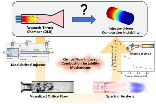
Orifice Flow Dynamics in a Rocket Injector as an Excitation Source of Injector-Driven Combustion Instabilities

Institute of Space Propulsion, German Aerospace Center (DLR), D-74239 Lampoldshausen, Germany
*
Author to whom correspondence should be addressed.
Current affiliation: Institut für Thermodynamik, Fakultät für Luft- und Raumfahrttechnik, Universität der Bundeswehr München, D-85577 Neubiberg, Germany.
Aerospace 2023, 10(5), 452; https://doi.org/10.3390/aerospace10050452
Submission received: 24 March 2023 / Revised: 8 May 2023 / Accepted: 10 May 2023 / Published: 15 May 2023
(This article belongs to the Special Issue Liquid Rocket Engines)

Abstract

:
To investigate a hypothesis of the orifice flow-induced instability in rocket engine thrust chambers, a single liquid oxygen (LOX) injector with an optically accessible orifice module was used for experiments, with water as a simulant for LOX. The unsteady pressure downstream of the orifice was measured using high-speed piezoelectric sensors under cavitating and non-cavitating intra-injector flow conditions. The cavitating orifice flows were directly visualized via backlight imaging with a high-speed camera through the optically accessible orifice module. Cavitation initiated at the cavitation number of 2.05, and the downstream bubble cloud formation started below 1.91. The unsteady pressure spectrum arising from cavitation comprises multiple peaks over a broad frequency range, which can cause low- and high-frequency instabilities. The dominant frequencies from cavitation decrease with increasing pressure drop, while the frequencies during non-cavitating flow increase. The non-cavitating orifice flow excites the second longitudinal acoustic mode of the injector tube. The acoustic mode excited by the non-cavitating flow becomes stronger when the pressure peak in the range of whistling phenomenon is close to the first longitudinal acoustic mode. In conclusion, the excitation mechanisms of the orifice-induced instability for the cavitating and non-cavitating flows were well identified, despite the limitations of water as a simulant for LOX.

Graphical Abstract

1. Introduction

Combustion instabilities in liquid rocket engines have been studied for a long time, but they are still one of the most critical design issues due to the variety of potential driving mechanisms [1]. In previous studies, the flow dynamics inside injector elements with orifices have been reported as the excitation source of the combustion instability under certain conditions. High-frequency (HF) instabilities of liquid oxygen/hydrogen (LOX/H 2 ) combustion were observed when the resonance mode of the LOX-post matched the first transverse acoustic mode (1T) in the combustion chamber of the research thrust chamber model ‘D’ (or “BKD”) [2,3,4] as shown in Figure 1. Armbruster et al. [3] concluded that the orifice whistling phenomenon at a Strouhal number of approximately 0.35 caused the excitation of the acoustic eigenmodes in the LOX injectors, which modulated the heat release rate, leading to an excitation of the 1T mode of the combustion chamber. However, because it was not possible to access the intra-injector flow during hot-fire tests with 42 injector elements, the conclusion was deduced via indirect observations, and confirmation of whistling in the LOX post is outstanding. A numerical study by Tsohas and Heister [5] suggested that hydrodynamic processes in the injector could potentially interact with and intensify acoustic oscillations, or result in modulated injection rates, influencing high-frequency combustion instabilities.
In addition, low-frequency (LF) instabilities were observed during tests with the same thrust chamber utilising liquid oxygen and liquefied natural gas (LOX/LNG) [6], which also seem to be related to the intra-injector flow. Strong LF instabilities arose during the start-up transient, as shown in Figure 2, corresponding to the time when the LOX flow across the injector orifice experienced a phase change with dropping LOX injection temperature and increasing pressure. Klein et al. [7] have also reported combustion instability of a LOX/GCH 4 combustor during the start-up related to the two-phase flow in the LOX orifice. Coupling of injector and chamber acoustic frequencies could be established by adopting the model of the speed of sound in a bubbly flow. However, these were again indirect observations used to analyze the two-phase flow induced combustion instability due to the lack of measurements within the injector.
From the previous hot-firing experiments, it can be deduced that the intra-injector flow dynamics play a significant role in combustion instabilities, but direct observation of the intra-injector flow is rare in the literature. Consequently, direct flow visualization of the orifice-induced resonance in the LOX injector is essential. There have been experimental [8,9,10,11,12,13] and numerical [14,15,16] studies focusing on the visualization of cavitation bubbles at orifices.
Hitt et al. [8] experimentally investigated the cavitation-induced instability across the orifice in the supply line of a cryogenic medium. They used liquid nitrogen as the simulant for LOX. During the experiments, fluctuations from 153 to 275 Hz were observed, and the researchers concluded that the cavitation at an orifice could potentially trigger LF instabilities, also known as ’chugging’. Sato and Saito [9] visualized cavitation bubbles in a circular orifice and classified unsteady behaviors of the cavitation during the growth, coalescence, shedding and collapse phases. Sugimoto and Sato [10] tried to find periodical characteristics with streak records of bubbles. Since the bubbles can visualize the flow, cavitation bubbles have been analyzed both experimentally [11,12,13] and numerically [15,16] using spectral analysis methods to detect periodic fluctuating characteristics. Esposito et al. [11] obtained periodic modes from the images using the proper orthogonal decomposition method, finding dominant modes at Strouhal numbers of 0.4 and 0.9 The Strouhal number ( S t ) is defined as shown in Equation (1), where f is the frequency, δ is the orifice thickness and U d is the bulk velocity at the orifice.
S t = f δ U d
Flow-induced noise, known as ‘pipe-tone’ [17] or ‘whistling phenomenon’ [18], can also cause the unstable response downstream of an orifice without cavitation. The whistling across orifices is observed at Strouhal numbers in the range of 0.2 to 0.4 [18,19]. Numerical simulations also have been conducted and have illustrated the periodical fluctuation from the flow separation at the orifice wall [19,20]. In a recent study, Son et al. [21] showed evidence of the flow-induced resonance of the LOX post by using large-eddy simulation (LES) of the LOX post. Even though the simulation was conducted without any external modulation, the longitudinal mode of the LOX post was excited by the orifice flow. In addition, the pressure mode at the Strouhal number of 0.38 presented very strong 1L-like fluctuation, and this Strouhal number is in the range of whistling. The orifice-induced flow-acoustic resonance was also reproduced through acoustic analysis. Brokof et al. [22] developed a modeling approach based on the linearization of the compressible Navier–Stokes equations for the orifice length-to-diameter range of 1.5–3.0, demonstrating that medium-sized holes whistle at higher Strouhal numbers than short holes, and highlighting the importance of accurately modeling vorticity growth at the orifice in the semi-analytical model.
Even though several experimental studies on flow-induced fluctuation have been conducted [8,11,17,18,23,24,25,26], resonance effects with the LOX post volume downstream of the orifice have not been addressed. Moreover, even though numerical studies showed evidence of the whistling-related flow excitation, experimental validation of intra-injector flow dynamics is largely lacking.
In this work, an experimental study is conducted with a single injector tube and water as a simulant for LOX to directly observe the intra-injector flow dynamics. Using high-speed imaging, periodical bubble behaviours were observed at high cavitation numbers. Through spectral analyses of the high-speed images and the unsteady pressure records, fluctuations are analyzed at various flow conditions to understand the modal characteristics of the cavitating and non-cavitating flows in the injector tube.

2. Experimental Setup and Methods

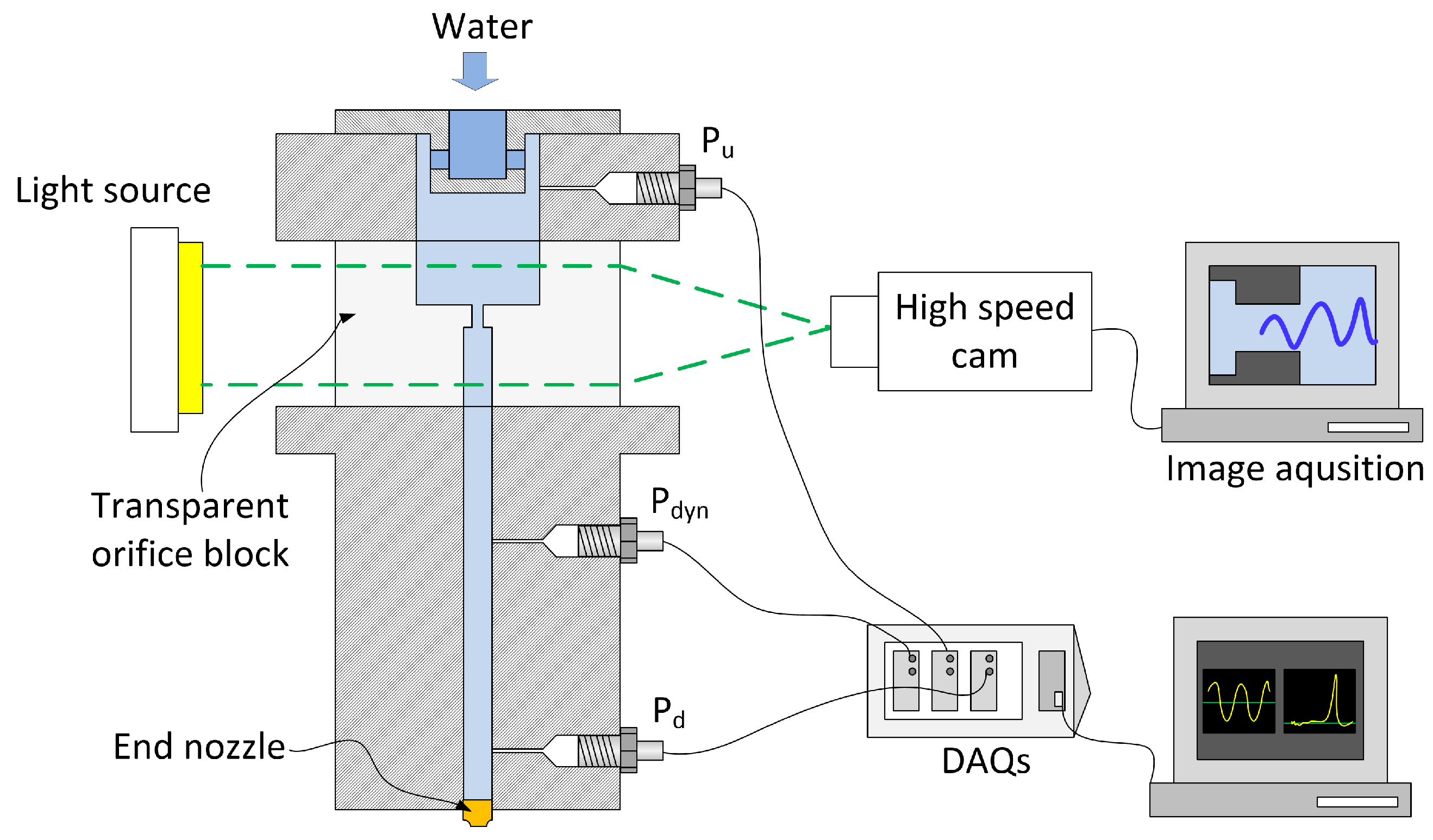
2.1. Experimental Setup and Modular Injector Tube

The experimental setup is configured as shown in Figure 3. The modular injector consists of three parts: the supply manifold, the optically accessible part, and the downstream part with pressure taps and a nozzle which defines the pressure loss at the outlet of the injector. Detailed geometries and dimensions are illustrated in Figure 4. Two different flow conditions at the orifice are considered: Cavitating flow and non-cavitating flow. This is achieved by using different nozzles at the end of the injector tube. The nozzle element N035 has a 3.5- m m hydraulic diameter, which is close to the 3.6- m m tube diameter, whereas N015 has a 1.5- m m hydraulic diameter.
The transparent block which includes the orifice is manufactured from acrylic glass (Polymethyl methacrylate; PMMA). The dimensions of the orifice are the same as in the actual LOX post of the reference injector of the hot-fire experiment (BKD) [3], as shown in Figure 4a. A BKD injector is a shear-coaxial type injector, which injects LOX through the central cylindrical tube and H 2 through the annular gap. The length of the LOX post is 68 mm, and the inner diameter of the LOX posts is 3.6 mm. The injector is internally recessed by 2-mm. The LOX injector features a plain orifice-shaped throttle with a 45-degree chamfer at the inlet, which maintains an appropriate pressure drop to increase the instability margin [1].
The LOX injector model in this study was designed as shown in Figure 4b, preserving the original dimensions of the orifice and the diameter of the LOX tube. A chamfer on the orifice inlet edge of 0.5 m m was realized at 45 degrees. The tube downstream of the nozzle is 204 m m long, which is three times longer than the original LOX injector in BKD, reducing the longitudinal mode frequency of the tube with water simulant, as shown in Table 1. This scaling is required to simulate the orifice flow condition of the hot-firing test. The nth-order longitudinal mode ( f L , n ) can be calculated using Equation (2), assuming an open–open tube [2]. c represents the speed of sound and L e f f is the effective length, which contains the downstream tube length, the orifice thickness, and the end nozzle length.
f L , n = n c 2 L e f f
The downstream unsteady pressure, P d y n , was measured with 100 k S / s using a piezoelectric sensor (Kistler A601) to detect the fluctuation from the flow after the orifice. Upstream and downstream static pressures— P u and P d , respectively—were measured using static pressure sensors (Kistler 4043). The sensors were distantly mounted with 1 m m -diameter measuring passages because the LOX tube was narrow compared to the sensor tip diameter. The estimated Helmholtz frequency from the pressure tap is approximately 9.3 k Hz . Because this frequency is far from the range of interest, the resonance effect from the pressure tap was negligible, as described in the following sections. Water was supplied by a pressurized tank, and the flow rate was measured using a turbine flow meter (Vision 2006 2F66). The pressure signals were collected via a data acquisition system (NI PXIe-1071).
A Photron UX100 camera and a diffusive flat LED panel were used for high-speed backlight imaging of the cavitating flow. The camera was synchronized by the data acquisition system. The frame rate of 40,000 f / s and the exposure time of 1 μs was used. The imaging was only performed for the cavitating flow, as the seeding method was not used for the non-cavitating flow to prevent acoustic disturbance from seeding particles.

2.2. Experimental Conditions

In this study, two flow conditions were considered to simulate two types of the injector-driven combustion instability scenarios; a cavitating flow for the LF combustion instability and a non-cavitating flow for the HF combustion instability. Downstream pressure was adapted using the two exit nozzle types (N015 or N035) to control the cavitation inception. The occurrence of cavitation is estimated by the definition of the cavitation number σ , as shown in Equation (3) [27], where P u represents the upstream pressure, P d is the downstream pressure, and P v is the saturation pressure. In this study, a P v of 2.34 k Pa for the water at 293 K is used to calculate the cavitation number, and the temperature sensitivity of the cavitation number is less than ±1% within ±5 K .
σ = P u P v P u P d
Cavitation inception is expected to occur at cavitation numbers from 1.8 to 2.2, according to the diameter ratio of the orifice to the downstream tube [28]. When the N015 nozzle is used, the global cavitation numbers at all pressure drop conditions are much higher than 2.0, as shown in Figure 5, whereas the global cavitation numbers with the N035 enter the potentially cavitating ranges below 2.0.

3. Results and Discussion

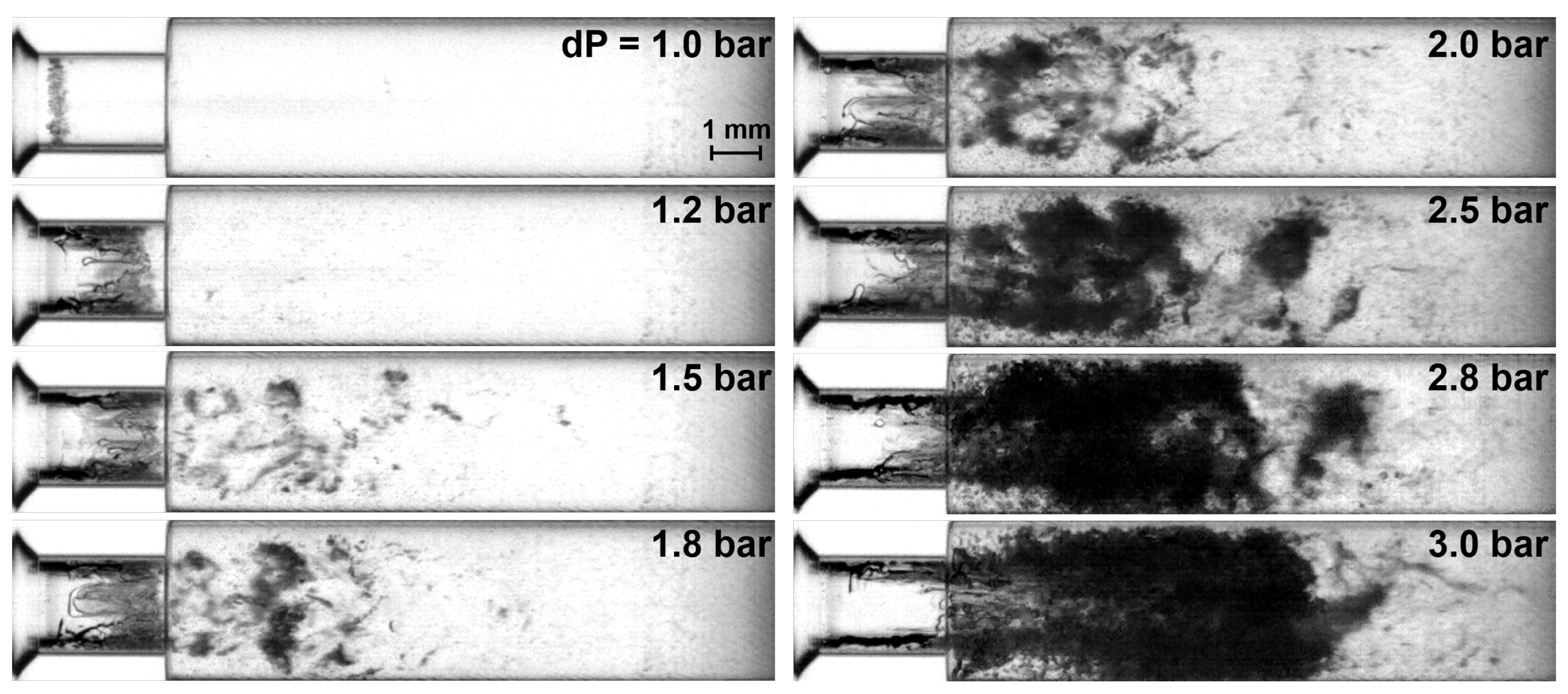
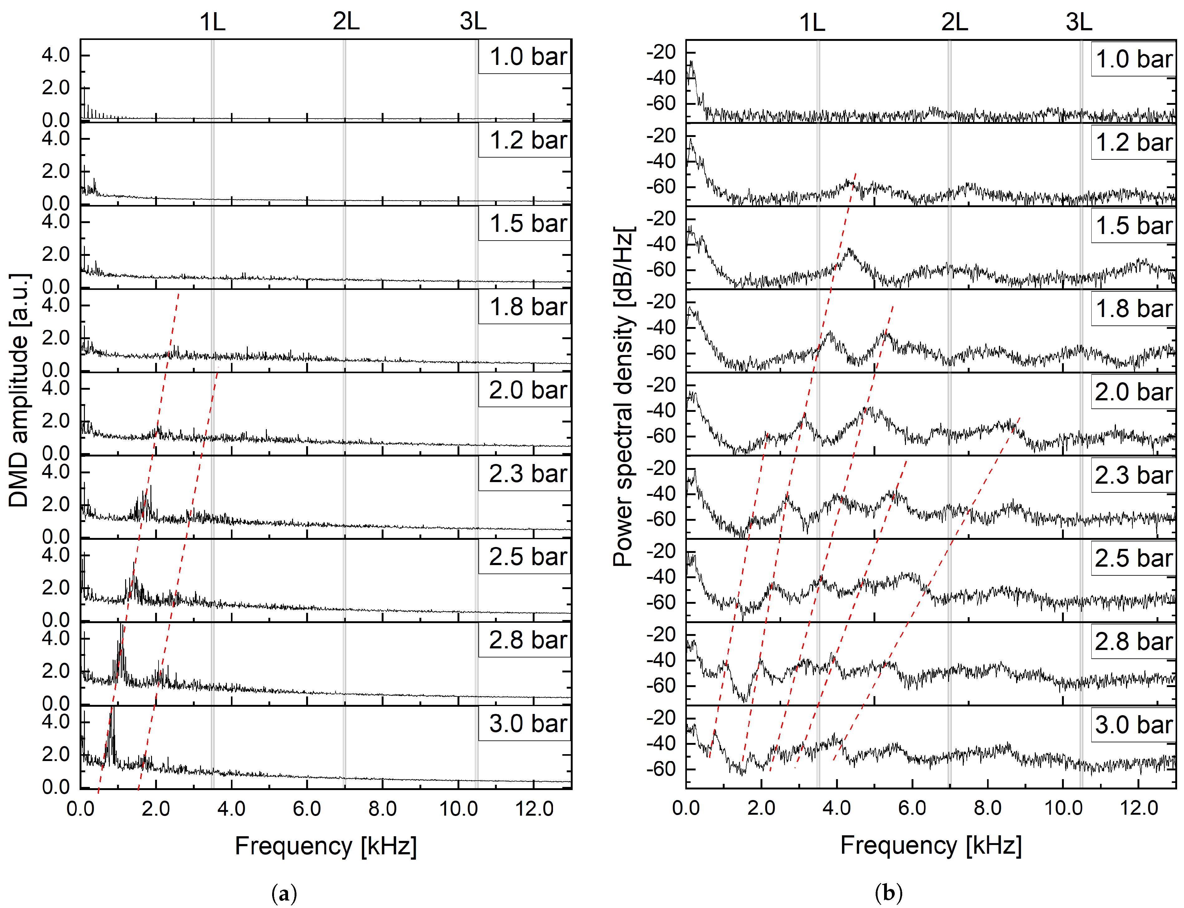
3.1. Periodic Fluctuation of Cavitating Flow

When the pressure drop increases from zero bar with the N035 nozzle, the cavitation is initiated quickly at 0.8–0.9 bar, and then the stable bubbly flow is maintained with a 1.0-bar pressure drop at the edge of the orifice inlet with small nucleation bubbles, as shown in Figure 6. At a 1.0-bar pressure drop the cavitation number is 2.07, which is similar to the cavitation limit of 2.05 in the study by Yan and Thorpe [28] for an orifice diameter ratio of 0.56. The bubble length grows with the increasing pressure drop up to 1.2 bar, corresponding to a cavitation number of 1.91, but the bubbles vanish before reaching the orifice outlet. When the pressure drop is higher than 1.2 bar, the cavitation bubbles are released into the injector tube across the orifice outlet, which generates the bubble clouds.
To analyze the periodicity of the bubbly flows, power spectral densities (PSD) of the acoustic pressures in the injector tube were obtained from the unsteady pressure sensor, and spectral modes of bubble clouds captured by the high-speed camera were analyzed by a dynamic mode decomposition (DMD) [29,30]. Because the description of the DMD is only briefly presented here, a more detailed description can be found in the references provided.
In order to reconstruct the flow field at specific mode frequencies later, the collected data X ( t ) have the mean data X ¯ subtracted at first, and then the resulting fluctuation data X ( t ) are used for DMD analysis. The size of X is m × n , where m is the number of snapshot pixels rearranged in a single column and n is the number of sequential images, which represents temporal evolution t. The fluctuation data are divided into two datasets: The current state X n 1 , which contains the snapshots from 1 to n 1 time steps, and the future state X n from 2 to n time steps. From DMD analysis, it is assumed that X n 1 and X n have a linear relation, as shown in Equation (4), where A is a linear dynamical system.
X n = A X n 1
X n 1 can be decomposed using singular value decomposition (SVD), as follows: X n 1 = U Σ V * . However, the spatial resolution m is usually much larger than the number of images n. Therefore, a reduced SVD can be applied [31], as shown in Equation (5), where Σ r is an n × n matrix.
X n 1 = U r Σ r V r *
From the relation of = A X n 1 X n , the pseudo-inverse of X n can be calculated by SVD as Equation (6).
X n = V r Σ r U r *
Then, the reduced linear dynamical system A ˜ can be calculated using Equation (7), where A ˜ = U r * A U r .
A ˜ = U r * X n V r Σ r 1
The spatial DMD mode, denoted as Φ , is calculated using Equation (8) and is based on the eigenvalue decomposition, as presented in Equation (9). W corresponds to the set of eigenvectors, while Λ represents the set of eigenvalues.
Φ = X n V r Σ r 1 W
A ˜ W = W Λ
The original fluctuation data X ( t ) can be reconstructed using Equation (10), where Ω = log Λ , b is the mode amplitude, and the original dataset is X ( t ) + X ¯ .
X ( t ) = Φ e Ω t b
For each DMD mode, the DMD mode frequency ( f D M D ) in Hz and the amplitude (b) can be derived as follows, where ν is the frame rate of the high-speed camera and Φ is pseudo-inverse of Φ .
f D M D = | ν Ω | 2 ϕ
b = Φ X ( 1 )
By comparing mode frequencies and amplitudes, we can obtain the DMD spectra and identify a specific mode μ with a high amplitude, which contains the dominant fluctuating mode. Furthermore, X ( t ) μ can be obtained using Equation (13), which represents the reconstructed sequential flow images with the fluctuation at the specific frequency. To clearly observe the effect of the specific fluctuation on the mean flow, a weighting factor C w can be applied; the factor of 10 was applied in this study.
X μ ( t ) = X ¯ + C w Φ μ e Ω μ t b μ
According to the DMD analysis, the peak frequencies can be captured from the flow, which are compared with power spectral densities of pressure measured at the end of the injector tube downstream. As shown in Figure 7a, strong peaks appear in the dynamics of the visualized bubble field at near 1 to 2 k Hz and weak harmonic peaks are also observed. Similar peaks are observed in the pressure spectra in Figure 7b, with more harmonic peaks appearing than in the DMD results. Therefore, it is clear that the cavitating flow generates a strong pressure oscillation in the downstream part of the injector tube.
There are two meaningful characteristics to be observed in Figure 7. First, the major peak frequency decreases as the pressure drop increases. This results from the increase in the bubble-cloud length as the pressure drop increases. It can be identified by comparing the trends of bubble length and peak frequencies according to the change in the pressure drop. Based on the mean flow images, the pixel intensity along the axis can be obtained, as shown in Figure 8. Because the bubble clouds emerge from the orifice when the pressure drop is above 1.5 bar, the images at lower pressure drops were excluded. The bubble-cloud length L b was defined as the inflection point of the intensity profiles, marked with hollow squares in Figure 8. The inflection points were derived from 5th-order polynomial fits. Comparing the bubble-cloud lengths and the secondary peak frequencies from Figure 7b at various pressure drops, it is clear that both are linearly related to the pressure drop, and the length is inversely proportional to the frequency, as shown in Figure 9. Thus, this result shows that the LOX-post excitation from the cavitation is related to the bubble length or the bubble lifetime from the orifice.
Second, the pressure peaks have multiple harmonics. This characteristic can be also observed from the hot-fire test records, as shown in Figure 2. The presence of multiple harmonics over a wide range of frequencies increases the chances of coupling with resonance of other components, such as combustion chamber acoustic modes. The red dashed lines in Figure 7a are matched with the first two lines in Figure 7b. The secondary pressure peak marked by the second red dashed line in Figure 7b is already excited at the pressure drop of 1.2 bar, though the bubble clouds do not yet extend past the orifice outlet (Figure 6). This means that the secondary peaks do not originate from the bubble clouds. In contrast, the primary pressure peak arises later than the DMD peak when the pressure drop reaches 2.3 bar. This means that the primary peak is more likely related to the bubble clouds exhausted from the orifice. This characteristic can be analyzed further using the DMD spatial modes.
From spatial modes of the cloud cavitation fluctuation, we can understand how the fluctuation occurs at specific frequencies. The pressure and DMD spectra for the 3.0-bar pressure drop, for example, are shown in Figure 10. The primary and secondary peaks from both results are well matched, as previously mentioned. At this condition, the spatial modes at these two frequencies, 880 and 1680 Hz , can be derived from the DMD, as shown in Figure 11. Left-side figures denote the DMD spatial modes from Equation (8) and right-side figures are the reconstructed flow images at corresponding frequencies via Equation (13). Both are arranged as sequential phases ϕ in a single period.
The bubble clouds fluctuate in the longitudinal direction, which can deliver the pressure oscillation downstream. The 880- Hz fluctuation is strongest, including the inner orifice flow, as shown in Figure 11a. When we see the spatial mode in the orifice, the entire flow resonates with the injected bubble clouds, and the position of the recirculation zone at the step after the orifice is also modulated. Because of the early detached flow at the orifice wall, lots of bubbles are generated inside the orifice, and they make the image blur at Φ = 0 . Afterwards, the bubbles are strongly injected into the shear layer of the bubble jet, as the arrow designates. Then, the bubbles return back to the orifice side due to the recirculation at ϕ = π / 2 , while the main bubble jet starts to stretch. Simultaneously, the detached boundary layer inside the orifice becomes stable. At ϕ = π , the bubble clouds still stretch and the boundary layer at the orifice wall becomes unstable from the orifice outlet. The bubble cloud stretches to the maximum extent at ϕ = 3 π / 2 , and begins the collapsing phase due to the pressure recovery escaping the vena contracta as the boundary layer detaches further. This mode has the lowest frequency because the flow resonates along the whole length of the bubble clouds.
The mode of the secondary peak at 1680 Hz shows different behaviour. This mode also shows the fluctuation originated from the boundary layer inside the orifice, but it is more likely related to smaller fluctuations in the boundary layer. As the arrow in Figure 11b designates, the thick boundary layer in the reconstructed flow is more clear to observe than in the 880- Hz flow and it pumps out separated bubble lumps to downstream. In this mode, the boundary layer is not fully detached but partially attached and it fluctuates as wrinkling curtains. It has very small movements but strongly affects the downstream flow. Because the wrinkling is faster than the pumping flow in the orifice at 880 Hz , the frequency is higher and the wavelength of the bubble clouds is shorter. It is similar to the flow fluctuation in the CFD results for the high-pressure LOX flow studied by Son et al. [21], and we can hypothesize that the whistling mechanism works in a similar way. However, note that the cavitating flow differs to non-cavitating flow because the pressure waves delivered downstream affect the local growth and collapse of bubble clouds. This allows strong multiple harmonics of pressure peaks, as shown in Figure 10. In addition, since this mode is caused by the flapping boundary, this mode can appear earlier than the primary mode, as shown in Figure 7a even though the bubble clouds downstream are not yet formed.

3.2. Periodic Fluctuation of Non-Cavitating Flow

To observe the pure hydrodynamic effects from the unsteady pressure records, the N015 end nozzle was used to increase the downstream pressure and avoid cavitation. Spectra of the unsteady pressure were analysed under various flow conditions, which are displayed in Figure 12a. Two strong peaks appear; the primary peak below 3 k Hz and the secondary peak near 7 k Hz . Because the frequency of the primary peak increases with increasing pressure drop, and thus flow velocity, it is likely that this primary peak is originating from the orifice flow. However, the most noticeable difference between cavitating and non-cavitating flows is in the trend of the primary peak frequencies. The peak frequencies increase according to increasing pressure drop, as seen in Figure 12a, whereas the peak frequencies of the cavitating flow decrease. This means that the dynamics of the non-cavitating flow have a different mechanism to the cavitating flow.
Whereas the bubble cloud length affects the excitation frequency in the cavitating flow, as described before, it seems the orifice flow velocity is the more relevant factor for the excitation from the non-cavitating flow, as shown in Figure 13. The orifice flow velocity is calculated based on the measured flow rates, the assumed water density, 1000 k g   m 3 , and the orifice area. The primary peak frequency is directly proportional to the orifice flow velocity. According to the CFD results presented by Son et al. [21], the boundary flow inside the orifice exhibited flapping behavior under non-cavitating flow conditions. This indicates that as the flow velocity through the orifice increases, the flapping speed of the boundary flow at the orifice wall also increases. As shown in Figure 12b, this characteristic can be normalized by the definition of the Strouhal number, which is defined as Equation (14), where the frequency from Equation (1) is replaced by the flow spectral frequency f f l o w from the pressure spectra. As a result, the primary peaks are observed in the range of typical whistling Strouhal numbers (0.2–0.4) [18,19].
S t f = f f l o w δ U d
The other significant observation is that the secondary peak near 7 k Hz starts to appear at 2.5-bar pressure drop, which is close to the second longitudinal mode (2L) of the LOX post resonance of 7.2 k Hz . This is an interesting phenomenon because the 2L injector mode is excited while only the primary peak is in the range of whistling. This finding strongly supports the claim made by Armbruster et al. [3] that the instability in BKD is caused by whistling from the orifice, which excites the resonance mode in the injector tube.
We can define the frequency difference Δ f between the 1L injector mode frequency f 1 L , p o s t and the primary peak frequency f p as Δ f = f 1 L , p o s t f p . We can compare Δ f and the deviation of the filtered pressure signal in the range of 6.0–8.0 k Hz , as shown in Figure 14. The deviation indicates the oscillation amplitude of the injector 2L mode. When the primary peak is close to the 1L mode frequency, the amplitude of the 2L mode becomes stronger. It can be expected that the strongest 2L mode can be obtained when both peaks are matched. This can explain why the BKD campaign had a strong 2L LOX injector mode; BKD had a strong peak at the 1L LOX injector mode, and this peak was in the range of whistling [3]. Based on the asymptotic assumption for the change in the 1L mode Strouhal number, both peaks can be matched at a Strouhal number of 0.4, whereas the BKD had the Strouhal number of 0.35.
In conclusion, we can determine the conditions required for the orifice-induced 2L resonance of the injector tube, which can cause HF combustion instability when the 2L injector mode matches the chamber mode. The injector should have an orifice that can create a whistling effect. The pressure drop across the orifice should be appropriate to generate a whistling pressure peak. Additionally, this peak should be close to the first longitudinal resonance mode downstream. This will cause the second longitudinal mode to occur, which could lead to the injector-induced combustion instability when the injector mode is matched with the combustion chamber mode.

3.3. Discussion

Adopting cavitating flow characteristics in water to simulate tests with LOX has limitations due to thermodynamic effects during bubble growth [32]. However, it seems that this mainly affects the bubble lifetime and the frequency estimation. Therefore, the accuracy can be affected but the mechanism will be valid.
Because water at room temperature has very low compressibility compared to LOX at 110 K and high pressure, the behaviour of the boundary layer at the orifice may differ, as will the acoustic damping of the medium. This might explain the Strouhal number of 0.4 for the maximum resonance observed in this work, which is higher than the value of 0.35 obtained in the original BKD experiments. Furthermore, the acoustic impedance of inlet and outlet conditions cannot be same as the actual LOX injector. However, indirect measurements of the LOX temperature and the injector tube pressure from the BKD could also affect the accuracy of the experimental results.
The results in this study are consistent with the observations in BKD, particularly the excitation of the 2L injector mode from whistling matched with the 1L injector mode. However, it was not clearly revealed in this study why the 2L injector mode was excited instead of the 1L mode. This could be explained by further studies, such as acoustic analysis.

4. Conclusions

In this study, we targeted mimicking two different combustion instability phenomena, which are potentially caused by the liquid oxygen (LOX) injectors in liquid propellant rocket combustors. Because only indirect measurements were possible in previous hot-fire tests, this study focused on direct measurements in the injector tube. The results showed similar behaviour as in the hot-fire tests and explained the mechanisms of the injector-related combustion instability in hot-fire tests.
To investigate the intra-injector flow characteristics of LOX injectors, a simplified modular injector with optical access was tested using water as a simulant under two different conditions: cavitating and non-cavitating flow conditions. For the cavitating flow, cavitation bubbles were captured using high-speed backlight imaging, and the captured images were analyzed using a dynamic mode decomposition (DMD) method. Primary and secondary frequency peaks from unsteady pressure spectra were observed in the DMD results. The primary peak was related to the cavitation bubble clouds downstream, whereas the secondary peak originated from flapping boundary layers inside the orifice. The cavitating flow showed a decrease in peak frequency with increasing pressure drop and multiple harmonics, which can easily match the resonance modes of other parts, such as a combustion chamber. This can explain the low-frequency combustion instability with multiple pressure peaks from the LUMEN campaign.
On the other hand, the non-cavitating flow showed an increase in peak frequency along with the pressure drop, and the peaks were observed in the range of whistling frequencies. The frequency increase was proportional to the flow velocity across the orifice. This indicates a hydrodynamic origin of the first peak frequency for the non-cavitating flow. The primary peak of the unsteady pressure from the non-cavitating flow was in the range of the whistling phenomenon. It was concluded that the second injector acoustic mode was excited when the whistling frequency peak was close to the first longitudinal acoustic injector mode. This finding is consistent with the hypothesized mechanism driving the high-frequency combustion instability observed during the BKD hot-fire tests.
The use of water as a LOX-simulant limited the comparability to observed phenomena during hot-run tests. Nevertheless, the results in this study successfully described the flow conditions in which combustion instabilities can be caused by cavitation and whistling of the LOX injector.

Author Contributions

Conceptualization, M.S. and J.S.H.; methodology, M.S.; software, M.S.; validation, W.A. and J.S.H.; formal analysis, M.S., M.B. and W.A.; investigation, M.S. and M.B.; resources, M.B.; data curation, M.S.; writing—original draft preparation, M.S.; writing—review and editing, M.S., M.B., W.A. and J.S.H.; visualization, M.S.; supervision, J.S.H.; project administration, J.S.H. All authors have read and agreed to the published version of the manuscript.

Funding

This activity was performed in the frame of the DLR internal project LUMEN.

Data Availability Statement

The data presented in this study are available on request from the corresponding author.

Acknowledgments

Authors thank Arthur Walz-Steinbach, Jonas Vogel, Markus Dengler and Michael Zepmeisel for the technical support.

Conflicts of Interest

The authors declare no conflict of interest.

References

  1. Sutton, G.P.; Biblarz, O. Rocket Propulsion Elements; John Wiley & Sons: Hoboken, NJ, USA, 2016. [Google Scholar]
  2. Gröning, S.; Hardi, J.S.; Suslov, D.; Oschwald, M. Injector-driven combustion instabilities in a hydrogen/oxygen rocket combustor. J. Propuls. Power 2016, 32, 560–573. [Google Scholar] [CrossRef]
  3. Armbruster, W.; Hardi, J.S.; Suslov, D.; Oschwald, M. Injector-Driven Flame Dynamics in a High-Pressure Multi-Element Oxygen–Hydrogen Rocket Thrust Chamber. J. Propuls. Power 2019, 35, 632–644. [Google Scholar] [CrossRef]
  4. Armbruster, W.; Hardi, J.; Oschwald, M. Impact of shear-coaxial injector hydrodynamics on high-frequency combustion instabilities in a representative cryogenic rocket engine. Int. J. Spray Combust. Dyn. 2022, 14, 118–130. [Google Scholar] [CrossRef]
  5. Tsohas, J.; Heister, S. Cfd simulations of liquid rocket coaxial injector hydrodynamics. In Proceedings of the 45th AIAA/ASME/SAE/ASEE Joint Propulsion Conference & Exhibit, Denver, CO, USA, 2–5 August 2009; p. 5387. [Google Scholar]
  6. Hardi, J.; Martin, J.; Son, M.; Armbruster, W.; Deeken, J.C.; Suslov, D.; Oschwald, M. Combustion Stability Characteristics of a sub-scale LOX/LNG Rocket Thrust Chamber. In Proceedings of the Aerospace Europe Conference 2020, Bordeaux, France, 25–28 February 2020. [Google Scholar]
  7. Klein, S.; Börner, M.; Hardi, J.S.; Suslov, D.; Oschwald, M. Injector-coupled thermoacoustic instabilities in an experimental LOX-methane rocket combustor during start-up. Ceas Space J. 2020, 12, 267–279. [Google Scholar] [CrossRef]
  8. Hitt, M.; Lineberry, D.; Ahuja, V.; Frederick, R. Experimental investigation of cavitation induced feedline instability from an orifice. In Proceedings of the 48th AIAA/ASME/SAE/ASEE Joint Propulsion Conference & Exhibit, Atlanta, GA, USA, 30 July–1 August 2012; p. 4029. [Google Scholar]
  9. Sato, K.; Saito, Y. Unstable cavitation behavior in a circular-cylindrical orifice flow. JSME Int. J. Ser. Fluids Therm. Eng. 2002, 45, 638–645. [Google Scholar] [CrossRef]
  10. Sugimoto, Y.; Sato, K. Visualization of unsteady behavior of cavitation in circular cylindrical orifice with abruptly expanding part. In Proceedings of the 13th International Topical Meeting on Nuclear Reactor Thermal Hydraulics, Kanazawa, Japan, 27 September–2 October 2009; Volume 13. [Google Scholar]
  11. Esposito, C.; Mendez, M.; Steelant, J.; Vetrano, M.R. Spectral and modal analysis of a cavitating flow through an orifice. Exp. Therm. Fluid Sci. 2021, 121, 110251. [Google Scholar] [CrossRef]
  12. Ge, M.; Petkovšek, M.; Zhang, G.; Jacobs, D.; Coutier-Delgosha, O. Cavitation dynamics and thermodynamic effects at elevated temperatures in a small Venturi channel. Int. J. Heat Mass Transf. 2021, 170, 120970. [Google Scholar] [CrossRef]
  13. Ge, M.; Manikkam, P.; Ghossein, J.; Subramanian, R.K.; Coutier-Delgosha, O.; Zhang, G. Dynamic mode decomposition to classify cavitating flow regimes induced by thermodynamic effects. Energy 2022, 254, 124426. [Google Scholar] [CrossRef]
  14. Egerer, C.P.; Hickel, S.; Schmidt, S.J.; Adams, N.A. Large-eddy simulation of turbulent cavitating flow in a micro channel. Phys. Fluids 2014, 26, 085102. [Google Scholar] [CrossRef]
  15. Brandao, F.L.; Bhatt, M.; Mahesh, K. Numerical study of cavitation regimes in flow over a circular cylinder. J. Fluid Mech. 2020, 885, A19. [Google Scholar] [CrossRef]
  16. Sadri, M.; Kadivar, E. Numerical investigation of the cavitating flow and the cavitation-induced noise around one and two circular cylinders. Ocean. Eng. 2023, 277, 114178. [Google Scholar] [CrossRef]
  17. Anderson, A. Dependence of Pfeifenton (pipe tone) frequency on pipe length, orifice diameter, and gas discharge pressure. J. Acoust. Soc. Am. 1952, 24, 675–681. [Google Scholar] [CrossRef]
  18. Testud, P.; Moussou, P.; Hirschberg, A.; Aurégan, Y. Noise generated by cavitating single-hole and multi-hole orifices in a water pipe. J. Fluids Struct. 2007, 23, 163–189. [Google Scholar] [CrossRef]
  19. Alenius, E.; Åbom, M.; Fuchs, L. Large eddy simulations of acoustic-flow interaction at an orifice plate. J. Sound Vib. 2015, 345, 162–177. [Google Scholar] [CrossRef]
  20. Lacombe, R.; Föller, S.; Jasor, G.; Polifke, W.; Aurégan, Y.; Moussou, P. Identification of aero-acoustic scattering matrices from large eddy simulation: Application to whistling orifices in duct. J. Sound Vib. 2013, 332, 5059–5067. [Google Scholar] [CrossRef]
  21. Son, M.; Armbruster, W.; Tonti, F.; Hardi, J. Numerical study of acoustic resonance in a LOX injector post induced by orifice flow. In Proceedings of the AIAA Propulsion and Energy 2021 Forum, Virtual Event, 9–11 August 2021; p. 3568. [Google Scholar]
  22. Brokof, P.; Guzmán-Iñigo, J.; Yang, D.; Morgans, A.S. The acoustics of short circular holes with reattached bias flow. J. Sound Vib. 2023, 546, 117435. [Google Scholar] [CrossRef]
  23. Abom, M.; Allam, S.; Boij, S. Aero-acoustics of flow duct singularities at low mach numbers. In Proceedings of the 12th AIAA/CEAS Aeroacoustics Conference (27th AIAA Aeroacoustics Conference), Cambridge, MA, USA, 8–10 May 2006; p. 2687. [Google Scholar]
  24. Moussou, P.; Testud, P.; Aure´gan, Y.; Hirschberg, A. An acoustic criterion for the whistling of orifices in pipes. In Proceedings of the ASME Pressure Vessels and Piping Conference, San Antonio, TX, USA, 22–26 July 2007; Volume 42827, pp. 345–353. [Google Scholar]
  25. Testud, P.; Aurégan, Y.; Moussou, P.; Hirschberg, A. The whistling potentiality of an orifice in a confined flow using an energetic criterion. J. Sound Vib. 2009, 325, 769–780. [Google Scholar] [CrossRef]
  26. Lacombe, R.; Moussou, P.; Aurégan, Y. Whistling of an orifice in a reverberating duct at low Mach number. J. Acoust. Soc. Am. 2011, 130, 2662–2672. [Google Scholar] [CrossRef] [PubMed]
  27. Kiesbauer, J. Control valves for critical applications. Hydrocarb. Process. 2001, 80, 89–100. [Google Scholar]
  28. Yan, Y.; Thorpe, R. Flow regime transitions due to cavitation in the flow through an orifice. Int. J. Multiph. Flow 1990, 16, 1023–1045. [Google Scholar] [CrossRef]
  29. Schmid, P.J. Dynamic mode decomposition of numerical and experimental data. J. Fluid Mech. 2010, 656, 5–28. [Google Scholar] [CrossRef]
  30. Kutz, J.N.; Brunton, S.L.; Brunton, B.W.; Proctor, J.L. Dynamic Mode Decomposition: Data-Driven Modeling of Complex Systems; Society for Industrial & Applied Mathematics: New York, NY, USA, 2016. [Google Scholar]
  31. Demmel, J. Singular value decomposition. In Templates for the Solution of Algebraic Eigenvalue Problems: A Practical Guide; Society for Industrial & Applied Mathematics: New York, NY, USA, 2000; pp. 135–147. [Google Scholar]
  32. Franc, J.P. The Rayleigh-Plesset equation: A simple and powerful tool to understand various aspects of cavitation. In Fluid Dynamics of Cavitation and Cavitating Turbopumps; Springer: Berlin/Heidelberg, Germany, 2007; pp. 1–41. [Google Scholar]
Figure 1. Spectrogram of unsteady pressure records and sequence diagram of BKD campaign; a gray region denotes the unstable condition. Modified and reprinted with permission from [3] © 2019 by Wolfgang Armbruster, Justin S. Hardi, Dmitry Suslov, and Michael Oschwald.
Aerospace 10 00452 g001
Figure 2. Spectrogram of unsteady pressure records and test sequence diagram of LUMEN campaign; a gray region denotes the unstable condition. Modified and reprinted with permission from [6] © 2020 by Justin S. Hardi, Jan Martin, Min Son, Wolfgang Armbruster, Jan Deeken, Dmitry Suslov, and Michael Oschwald.
Aerospace 10 00452 g002
Figure 3. Experimental setup for flow visualization and data acquisition.
Aerospace 10 00452 g003
Figure 4. Dimensions of original and model injectors. (a) BKD injector. Reprinted with permission from [3] © 2019 by Wolfgang Armbruster, Justin S. Hardi, Dmitry Suslov, and Michael Oschwald. (b) Model LOX injector tube and measurement positions.
Aerospace 10 00452 g004
Figure 5. Cavitation number vs. pressure drops.
Aerospace 10 00452 g005
Figure 6. Visualized cloud cavitation as increase of pressure drop.
Aerospace 10 00452 g006
Figure 7. DMD and pressure spectra of cavitating flow at various pressure drops. The red dashed lines indicate the trend of changing peak frequencies corresponding to variations in pressure drop. (a) DMD spectra of bubble clouds. (b) Power spectra of unsteady pressures.
Aerospace 10 00452 g007
Figure 8. Intensities of mean flow images along the axis at various pressure drops and bubble-cloud lengths ( L b ).
Aerospace 10 00452 g008
Figure 9. Comparison of bubble-cloud lengths and peak frequencies of unsteady pressures at pressure drops.
Aerospace 10 00452 g009
Figure 10. Spectra of unsteady pressure and DMD mode at d P = 3.0 bar.
Aerospace 10 00452 g010
Figure 11. DMD results at d P = 3.0 bar; (left) spatial modes and (right) reconstructed flow fields at a specific frequency. (a) Spatial modes at 880 Hz. The arrows designate the movements of cavitation bubbles within the recirculation zone at the corner. (b) Spatial modes at 1680 Hz. The arrow designates the location of the fluctuating bubble boundary layer at the orifice wall.
Aerospace 10 00452 g011
Figure 12. Spectra of unsteady pressures of non-cavitating flow. The red dashed lines indicate the trend of changing peak frequencies within the whistling range. (a) Power spectral density vs. frequency. (b) Power spectral density vs. Strouhal number.
Aerospace 10 00452 g012
Figure 13. Relation between primary peak frequencies and orifice flow velocities.
Aerospace 10 00452 g013
Figure 14. Standard deviations of filtered pressures at 6.0–8.0 k Hz according to differences between 1L mode frequencies and primary frequencies.
Aerospace 10 00452 g014
Table 1. Comparison of longitudinal mode (L) frequencies for a LOX injector tube.
CampaignBKD [3]Present
MediumLOXWater
Temperature ( K )112Room temperature
First longitudinal mode, 1 L ( k Hz )5.23.5
Second longitudinal mode, 2 L ( k Hz )10.47.0
Disclaimer/Publisher’s Note: The statements, opinions and data contained in all publications are solely those of the individual author(s) and contributor(s) and not of MDPI and/or the editor(s). MDPI and/or the editor(s) disclaim responsibility for any injury to people or property resulting from any ideas, methods, instructions or products referred to in the content.

