Article

Prediction of Aircraft Surface Noise in Supersonic Cruise State

1
School of Aeronautics, Northwestern Polytechnical University, Xi’an 710072, China
2
School of Civil Engineering, Chang’an University, Xi’an 710061, China
*
Author to whom correspondence should be addressed.
Aerospace 2023, 10(5), 439; https://doi.org/10.3390/aerospace10050439
Submission received: 2 March 2023 / Revised: 28 April 2023 / Accepted: 4 May 2023 / Published: 8 May 2023
(This article belongs to the Special Issue Aeroacoustics and Noise Mitigation)

Abstract

:
The aerodynamic noise of an aircraft leads to vibration fatigue damage to structures. Herein, a prediction method for aircraft surface noise under the comprehensive effect of mixed acoustic sources during flight, primarily surface aerodynamic, air intake, and tail nozzle jet noises, was studied. In the supersonic cruising state, the internal and external flow fields of the aircraft were solved using the Reynolds-averaged Navier–Stokes equations to obtain the statistical average solution of the initial turbulence. The non-linear disturbance equation was used to obtain the surface acoustic load of the aircraft. The calculation results revealed that the main source of aircraft surface noise is aerodynamic noise. The sound pressure level on the fuselage increases gradually from front to rear along the aircraft, and the OASPL at the air intake and tail nozzle is relatively large. The jet noise has little effect on the sound pressure level at the front of the fuselage and only contributes to the OASPL at the tail nozzle of the fuselage. The intensity of pressure pulsations from the engine exhaust in the tail section is 93.3% of the total intensity of pressure pulsations.

1. Introduction

Aircraft are subjected to severe dynamic loads during supersonic cruise and maneuvering flights [1]. To ensure the reliability of aircraft, it is necessary to perform acoustic and vibration environmental tests and determine the corresponding dynamic environmental conditions [2]. Using the traditional standard spectrum design method may incur unnecessary weight costs to the aircraft owing to the conservative design conditions, affect the performance of the aircraft, and lead to insufficient evaluation of airborne equipment owing to the untrue load environment, which results in serious hidden dangers to the aircraft [3]. The scientific and reasonable formulation of dynamic environmental conditions is highly significant for the development of aircrafts.
Since the 1970s, several experimental studies have been conducted on the aerodynamic noise of airframes. Through the analysis of large amounts of experimental data, empirical formulas between the aerodynamic noise of the airframe and aerodynamic shape, flight state, and flight conditions have been proposed and applied in engineering practises. For the aerodynamic noise of the entire aircraft, the main method still depends on semi-empirical methods of experimental measurement, which include aircraft flight and wind tunnel model measurements. For instance, the measurement of the G550 aircraft by Khorrami and Lockard [4] at the NASA Langley Research Centre confirmed that the aerodynamic noise of the airframe is the main source of an aircraft’s noise in the landing state. The wind tunnel model experiment was also improved. Stoker et al. [5] measured the noise of the Boeing 737 half model in the National Transonic Facility wind tunnel successfully, which was the first measurement of airframe noise in medium- and low-temperature environments. With the support of new experimental data, new semi-empirical methods are being developed. Blacodon [6] proposed a spectral estimation method (SEM) based on phased array measurement. Scarselli et al. [7] used a semi-empirical method based on the Engineering Sciences Data Unit (ESDU) database to calculate the airframe noise of civil transport aircraft.
By the 1990s, using powerful computational fluid dynamics (CFD) tools, researchers gradually found the distribution and changes of the flow field around the key structural components that produce aircraft noise and could systematically understand its generation and control mechanism; thus, aircraft noise prediction technology, which originally depended on experiments and empirical formulas, has developed to a higher level. NASA in the United States, DLR in Germany, and ONERA in France, in addition to various famous university research institutions and major aviation industry companies (such as Boeing and Airbus), have conducted extensive and in-depth research concerning aerodynamic noise. Through theoretical analysis, experimental research, and numerical calculation, a large number of research achievements have been made in aerodynamic noise prediction and calculation methods, generation mechanisms, tests and measurement technologies, and control technologies [8,9,10,11,12]. Currently, there is little research on numerical simulation methods to calculate the surface noise of the entire aircraft, and most of it is simulation research on single acoustic sources of the aircraft, such as the high-lift system [13], landing gear, jet of the nozzle [14], air intake, and the cavity of the internal weapon bay. The main numerical simulation methods include the direct calculation method and the acoustic analogy numerical simulation method. For the calculation of near-field noise, the direct numerical simulation method is often used. This method calculates the generation of the sound source and the radiation of the sound field by directly solving the unsteady N–S equations (DNS), large eddy simulation (LES), detached eddy simulation (DES), and the RANS equation.
One of the outstanding advantages of the direct calculation method is its high efficiency in dealing with near-field noise while taking into account the reflection, interference, and other physical phenomena of sound waves, which can help better understand the mechanism of noise generation and propagation. For mid- and far-field noise solving problems, in addition to the direct calculation method, according to Lighthill acoustic analogy theory, the flow field information at the near-field sound source can also be calculated by solving LES, DES, or unsteady Reynolds-averaged Navier–Stokes (URANS) equations [15,16,17,18,19], and then the acoustic wave equation can be used to solve the far-field noise problem. For instance, Pham et al. [20] studied the aerodynamic noise of the 2D high-lift wing configuration consisting of three components: the main wing, slat, and flap. He used a RANS steady-state solver for the mesh convergence study and verification of aerodynamic quantities and an LES unsteady-state solver for the aeroacoustic simulation problem. Lockard et al. [21] studied the slat noise source of a general high-lift configuration using the kω SST turbulence model and the Ffowcs Williams–Hawkings (FW–H) method. Daniel et al. [22] calculated leading-edge slat noise using the LES combined with acoustic perturbation equations. Ricciardi et al. [23] studied the noise predictions of realistic landing gear configurations combining high-fidelity CFD simulations and the FW–H acoustic analogy. Redonnet et al. [24] simulated the nose landing gear (NLG) noise physics through an advanced hybrid approach, which relies on CFD and Computational AeroAcoustics (CAA) calculations first. Then, the outputs coming from such CFD–CAA hybrid calculations are processed through both traditional and advanced post-processing techniques, thus offering to further investigate the NLG’s noise source mechanisms. Prasad et al. [25] used high-fidelity numerical simulations and experimental measurements in tandem to determine the amplitude and location of noise sources in heated supersonic jets. Good agreement was seen between the noise source locations using both LES and experimental data for the baseline jet. Shen et al. [26] analysed the broadband shock-associated noise using the simulation data of a heated, under-expanded supersonic jet from a high-order compressible LES solver. Yen et al. [27] achieved the resolution of the large-scale eddies of the cavity shear layer using a turbulence modeling method of Implicit Large Eddy Simulation (ILES) in which the numerical dissipations, including truncation errors and solution gradient-adaptive damping of the CESE method, take the place of an explicit sub-grid scale model, typically applied in an LES. Rodriquez et al. [28] studied the hypersonic cavity flow numerically using LES, DES, and IDDES approaches. Based on the primary results, it is anticipated that the IDDES will provide results comparable with LES at lower computational costs. The L/D ratio plays a key role in the boundary layer and shock development.
Based on the published literature the authors collected, it can be observed that there is no detailed simulation or research on the entire aircraft surface noise in the cruise process. The noise in the cruise state of the aircraft primarily includes surface aerodynamics, air intake, and tail nozzle jet noises. At present, designers mainly calculate noise according to different flow types of noise sources, which makes it difficult for them to accurately calculate the acoustic load of each subdivision position of the aircraft; therefore, the requirements of fine acoustic and vibration analysis of various parts of modern aircrafts cannot be met. Moreover, it is necessary to simulate the internal and external flow of the aircraft, which are different under different flight conditions. There are attached, separated, and vortex flows on the aircraft surface. Shock wave oscillations occur during supersonic flights [29,30]. Multi-flow coupling puts forward higher requirements for the calculation of the dynamic load.
The purpose of this study is to examine the entire aircraft’s surface noise in a supersonic cruise state under mixed acoustic sources. In Section 2, the numerical calculation methods are introduced, including the non-linear acoustics solver (NLAS) and its numerical solution. In Section 3, the M219 cavity and ARN2 nozzle are used to calculate the near-wall and jet noises, respectively, to verify the accuracy of the calculation method. In Section 4, the surface acoustic field of the aircraft’s flight at supersonic speed under mixed acoustic sources is calculated using the non-linear acoustics equation, and the accurate solution of the acoustic field at each position of the aircraft surface is obtained. In Section 5, the main conclusions of this work are summarised.

2. Non-Linear Acoustics Solver and Its Numerical Solution

The basic principle of the NLAS method is that the noise generated by large-scale vortices can be directly obtained by solving the non-linear disturbance equation (NLDE), whereas the small-scale turbulence that contributes to the sound source should be modelled to a certain extent. Unlike the DES method, the modelling of sub-grid scale turbulence is not based on the traditional effective eddy viscosity but on the calculation results of the RANS equation based on the statistical average, which is used for the synthesis of the sub-grid scale turbulence. The noise caused by the initial statistical average turbulence can be solved using RANS, and the non-linear acoustic solver is primarily used to simulate the generation and propagation of noise. The statistical average solution not only provides the basic characteristics of the average flow field but also presents a statistical description of the forced turbulence pulsation. Based on this statistical result, the non-linear acoustic solver reconstructed the acoustic source and simulated the propagation of pressure pulsation with high accuracy.
Solving aeroacoustic problems using the NLAS method can be divided into the following three steps: (1) solving the RANS equation to obtain the steady flow field; (2) synthesising the sub-grid scale turbulence based on the calculation results of the RANS equation; and (3) solving the NLDE and obtaining the sound field. Therefore, there are two key steps in the NLAS method: the establishment of the NLDE and the synthesis of sub-grid-scale turbulence based on the results of the RANS equation.
The NLAS method has low dissipation and can calculate the generation of noise at the sub-grid scale. The basic idea is that in the three-dimensional Cartesian coordinate system, assuming that a disturbance is added to the Navier–Stokes equations, each original variable is decomposed into statistical average and random disturbance variables, that is, φ = φ + φ’. The non-linear disturbance equation can be obtained by substituting it into the N–S equation and reorganising the N–S equation [31]:
q t + F i x i F i V x i = q ¯ t F ¯ i x i + F ¯ i V x i
where q is the transient disturbance, q ¯ is the transient average, F i is the linear inviscid perturbation, F ¯ i is the inviscid average (i = 1, 2, and 3, representing the x-, y-, and z-axis directions, respectively), F i V is the viscous disturbance, F ¯ i V is the viscous average, and xi is the distance in the direction of three coordinate axes: the x-axis, the y-axis, and the z-axis. The solution method for each item is shown in Equations (2)–(7).
q = ρ ρ ¯ u j + ρ u ¯ j + ρ u j e
F i V = 0 τ i j θ i + u k τ ¯ k i + u ¯ k τ k i
F i = ρ ¯ u i + ρ u ¯ i ρ u ¯ i u ¯ j + ρ ¯ u ¯ i u j + ρ ¯ u i u ¯ j + p δ i j u i e ¯ + p ¯ + u ¯ i e + p + ρ u i ρ ¯ u i u j + ρ u i u ¯ j + ρ u ¯ i u j + ρ u i u j u i e + p
q ¯ = ρ ¯ ρ ¯ u ¯ j e ¯ T
F ¯ i = ρ ¯ u ¯ i ρ ¯ u ¯ i u ¯ j + p ¯ δ i j u ¯ i e ¯ + p ¯
F ¯ i V = 0 τ i j θ ¯ i + u ¯ k τ ¯ k i
where the values of i, j, and k are 1, 2, and 3, respectively (1, 2, and 3 represent the x-axis, y-axis, and z-axis directions, respectively); ρ is the incoming flow density; u i ( u j , u k ) is the velocity of the disturbance along the x-axis (y-axis, z-axis); p is the pressure; e is the unit volume energy; δ i j is the Kronecker function; τ i j is the shear stress term; and θ is the heat conduction term. Omit density fluctuation and time-averaged Equation (1):
L H S ¯ = R H S ¯ = R i x i ,
with
R i = 0 ρ ¯ u i u j ¯ C p ρ Τ u i ¯ + ρ ¯ u i u k ¯ u ¯ k + 1 2 ρ ¯ u k u k u i ¯ + u k τ k i ¯ ,
where LHS and RHS represent the left and right terms of Formula (1), respectively; R i is the correlation between the standard Reynolds stress tensor and turbulent heat flux; C p is the pressure coefficient; T is the temperature; and * denotes averaging * .
To solve the NLDE, the values of these unknowns must be obtained, which can typically be acquired by solving the RANS equation. A small size that cannot be solved can be obtained by the artificial reconstruction method of turbulence and used to generate the sub-grid source term. After calculating the average statistical variable, the non-linear disturbance equation can be advanced. Kraichnan [32] proposed the earliest synthetic turbulence method in 1969; however, it is only applicable to isotropic turbulence. In 2001, Smirnov et al. [33] proposed a method based on the tensor scale so that the synthetic turbulence method could be applied to non-isotropic turbulence. Batten et al. [34] proposed a variant of the Smironv method in 2002, where the reconstruction formula for turbulent fluctuating velocity is as follows:
u i x j , t = a i k 2 N n = 1 N P k n cos d ^ j n x ^ j + ω n t ^ + q k n sin d ^ j n x ^ j + ω n t ^ ,
with
x ^ j = 2 π x j l , t ^ = 2 π t τ , d ^ j n = d j n l τ c n , p i n = ε i j k η j n d k n , q i n = ε i j k ξ j n d k n , η i n , ξ i n ~ N 0 , 1 , ω n ~ N 1 , 1 , d j n ~ N 0 , 0.5 ,
where l is the turbulence length, τ is the time scale, ε i j k is the permutation tensor of the vector product operation, C n is the velocity scale of the n-order mode, N α ,   β is the Gaussian normal distribution function with average α and standard deviation β and a i j is the Cholesky decomposition of the Reynolds stress tensor. For the symmetric positive definite Reynolds stress tensor u i u j ¯ , a i j can be solved using Equation (11):
a i j = u 1 u 1 ¯ 0 0 u 1 u 2 ¯ a 11 u 2 u 2 ¯ a 21 2 0 u 1 u 3 ¯ a 11 u 2 u 3 ¯ a 21 a 31 a 22 u 3 u 3 ¯ a 31 2 a 32 2 .
The solvable-scale vortex structure can be solved directly; the synthetic turbulence only provides non-solvable-scale information, so the large-scale vortex can be omitted; that is, Equation (10) should be filtered once. The filtering method ignores these modes that meet the conditions of L > d n L Δ ( L Δ . is the scale of the Nyquist grid), which also reduces the amount of calculation required to solve Equation (10) and saves computing resources.
In the unsteady calculation, the dual time step method was used; that is, the virtual time term was introduced into the control equation, and the physical time step was set according to the accuracy to solve the real solution. In each physical time step, convergence was achieved through iteration in virtual time, and multi-grid technology was applied to accelerate the convergence of the internal iteration step. The convection flux adopted the second-order accuracy Roe scheme, and the modified Venkata Krishnan limiter was selected to ensure second-order accuracy interpolation, which has the total variation diminishing property and small numerical dissipation. The diffusion flux was solved using a central difference scheme.

3. Method Verification

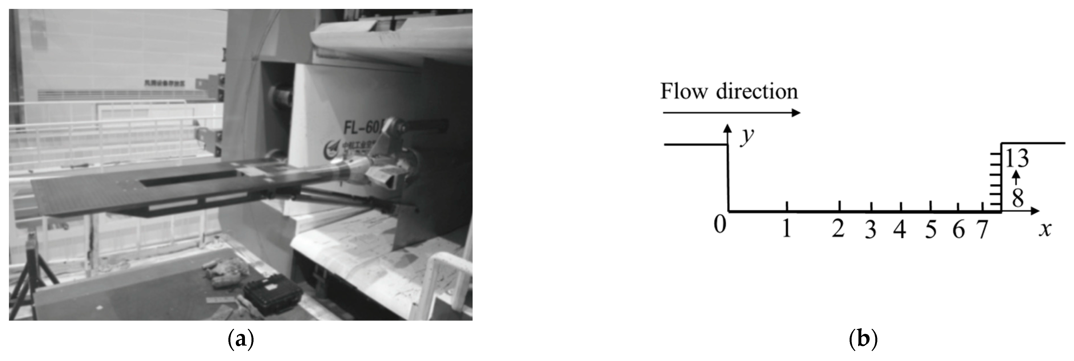
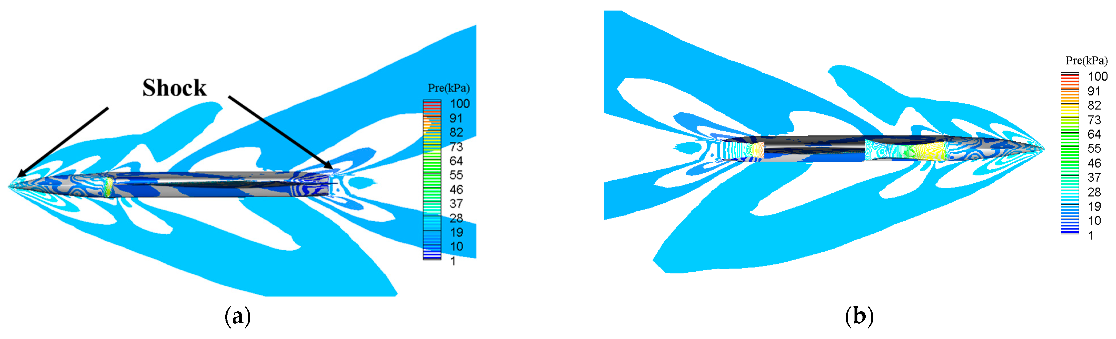
3.1. Verification of Near-Wall Noise Calculation

The calculation of aircraft surface noise is a near-wall noise calculation. The M219 cavity [35] was used to verify the near-wall noise calculated using the NLAS method. The 0.6 m × 0.6 m transonic/supersonic wind tunnel (FL-23) of the China Aerodynamics Research and Development Center was used for cavity noise measurement. The cavity for the wind tunnel test is an all-metal flat model, and the specific size is L × W × D: 508 mm × 101.6 mm × 101.6 mm, and the length–depth ratio of the cavity is five. Several pulsating pressure sensors were arranged at the bottom and rear walls of the cavity. The cavity experimental model and sensor position are shown in Figure 1, and the longitudinal and vertical positions of the relative cavity length and depth are listed in Table 1.
The experimental research primarily includes the flow characteristics of the cavity when Ma = 0.85 and Ma = 3.0. In this experiment, the sampling frequency of the fluctuating pressure acquisition system was 40 kHz, the sampling time was 5 s, the sampling was performed twice, the sample length was 4096, the number of samples was 48, the frequency resolution was 9.766 Hz, and the upper limit frequency was 20 kHz. The data signal acquisition system obtained the time domain information from the wind tunnel test and performed the Fourier transformation after the Hanning window correction to obtain the frequency domain information of the noise signal.
The cavity calculation domain and structured grid model are shown in Figure 2. The cavity noise was calculated under Ma = 0.85 and Ma = 3.0. The NLAS method is required to obtain the statistical average value of the flow volume by solving the RANS equation; therefore, the mesh division must meet the requirements of solving the RANS equation, and the thickness of the first layer of the mesh was 0.002 mm. The scale of the first layer of the grid on the wall of the IDDES method was 0.001 mm, making y+ approximately equal to 1.The CFD++ solver was used to compute. In the calculation of the IDDES method, the cavity wall was set as the adiabatic and non-slip wall. The farfield was set as the farfield Riemann invariant condition. The SST k–ω turbulence model was used for steady-state calculations. After the flow field was established and tended to stabilise, the IDDES method was used for unsteady calculations. According to the grid scale, the calculation time step was 2.5 × 10⁻⁶ s. The boundary condition settings of the NLAS method were the same as those of the IDDES method. The statistical average value of the flow variable was obtained by solving the RANS equation. When the flow field was stable, the calculation stopped, and the results were interpolated to the new acoustic calculation mesh. Subsequently, the NLAS method was applied to the new acoustic mesh for unsteady calculations; the unsteady calculation time step was 5 × 10⁻⁶ s.
The overall sound pressure level (OASPL) of the monitoring points in the cavity with Ma = 0.85 is shown in Figure 3. It can be observed from the figure that the OASPL calculated using the NLAS and IDDES methods is consistent with the experimental results, and the error is within 2 dB. Compared with the calculation results in other literature [36,37], the calculation accuracy of the NLAS and IDDES methods is similar to the DES method and slightly higher than the LES method. Figure 4 shows the experimental and simulation results for Ma = 3.0. The NLAS method accurately calculated the sound pressure level of the cavity noise within 5000 Hz. The peak value of the SPL and the frequency corresponding to the peak value were consistent with the experimental results, indicating the effectiveness of the NLAS method in the calculation of supersonic near-wall noise. The SPL calculated by the IDDES method decayed with an increase in frequency. The frequency corresponding to the peak value of SPL was consistent with the test results, but the peak values of SPL were not consistent with the test data.
Both the IDDES and NLAS methods can predict near-wall noise. At subsonic speed, the calculation errors of both of the two methods are within an acceptable range. At supersonic speed, the IDDES method introduces excessive dissipation in the process of information transmission at the junction of the LES and RANS, which leads to excessive dissipation in the process of sound wave propagation, resulting in a low predicted sound pressure level amplitude. In the NLAS method, the unsolvable scale turbulence is directly obtained using artificial synthesis, which avoids the additional dissipation brought by the transmission algorithm and gives it the characteristics of low dissipation. Consequently, the calculation of the noise propagation process is more accurate, and the obtained noise amplitude is closer to the actual physical value. In addition, the NLAS method has lower requirements for computational grids and physics time steps, which can save more computational resources and improve computational efficiency (as shown in Table 2). Accordingly, to predict aircraft surface noise by combining the advantages and disadvantages of the two methods, this study adopted the NLAS method in the cruise state.

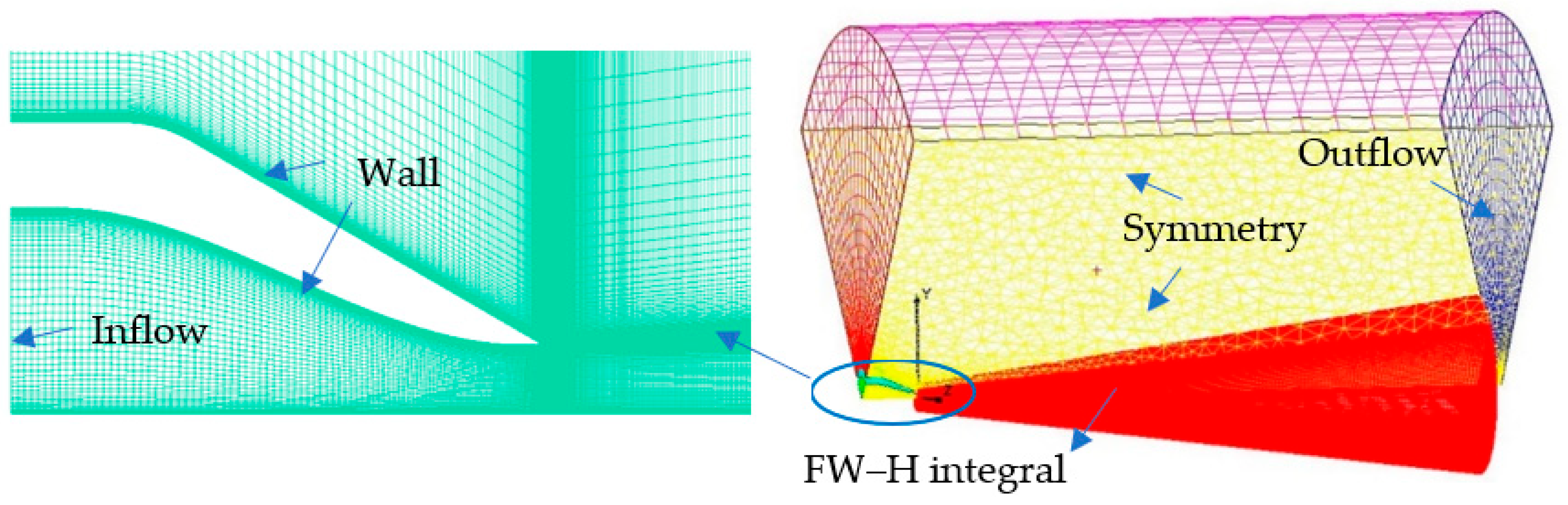
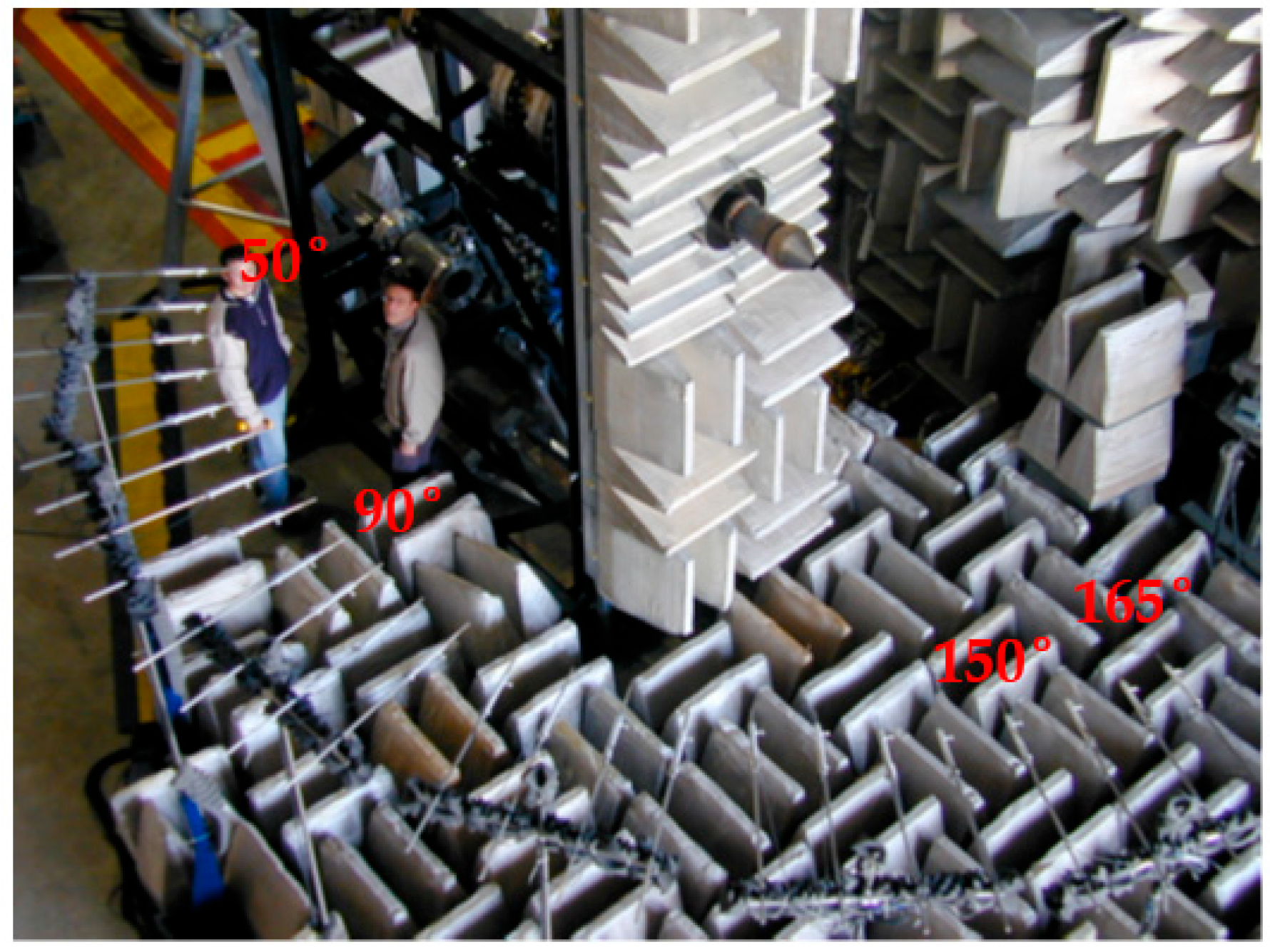
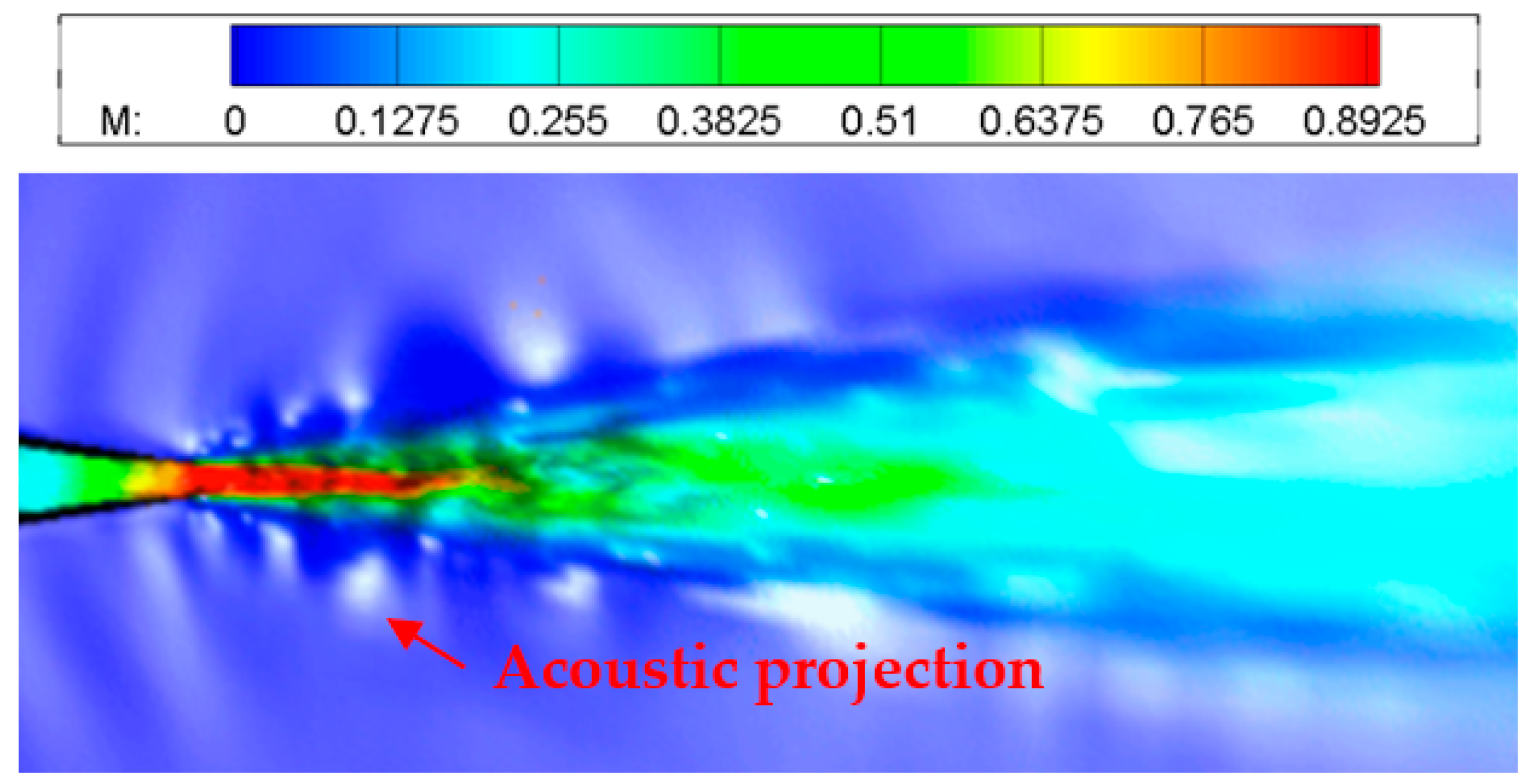
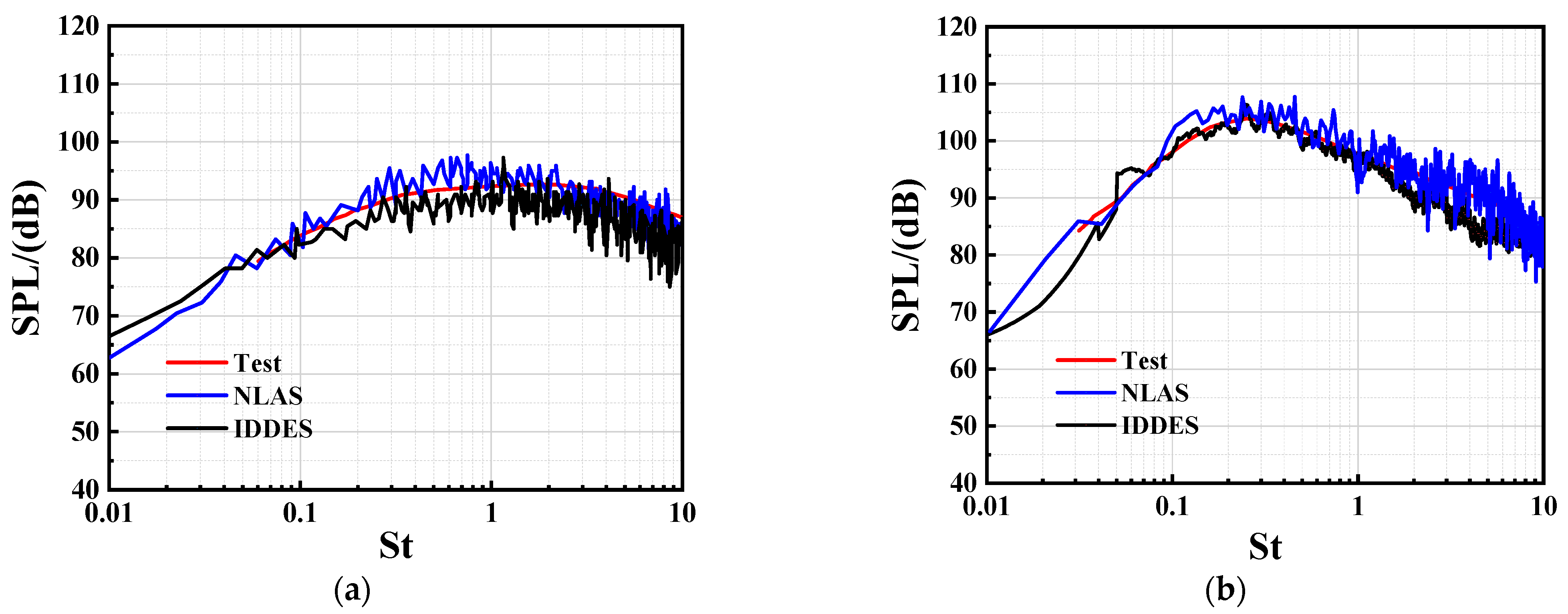
3.2. Verification of Jet Noise Calculation

The ARN2 acoustic reference nozzle developed by the NASA Glenn Research Centre [38] was used to verify the jet noise. It is an axisymmetric convergent nozzle with an outlet diameter of 2 inches. The 1/4 mesh model of the calculation domain and the nozzle mesh model are shown in Figure 5. The height of the first layer of the grid on the wall was 0.005 mm, making y+ approximately equal to one. When calculating the flow field, the inlet was the pressure inlet boundary, the outlet was the pressure outlet boundary, and the wall was adiabatic and non-slip. The near-field jet noise was solved using the NLAS and IDDES methods separately. When the NLAS method was used, the inlet and outlet were changed to the NLAS inlet/outlet boundary, and three absorption layers were added. The far-field noise was solved using the FW–H integral surface method. The mesh is refined in the direction normal to the wall, and the FW–H integral surface is refined compared to its surrounding space mesh.
The calculation conditions referred to relevant experiments on jet noise conducted by the NASA Glenn Research Centre. The experimental site and microphone monitoring points are shown in Figure 6 [38]. The microphone installation position angle was 50°–165°, a microphone was installed every 5°, and the distance was 40 times the nozzle outlet diameter. The Mach number at the outlet of the simulation calculation model was 0.9, the jet exit static-to-chamber static temperature ratio was Tr = 0.835, and the Reynolds number at the outlet of the nozzle was 2 × 10⁵.
The cloud diagram of the axial velocity of the nozzle calculated by the simulation is shown in Figure 7. The air velocity near the nozzle was the highest, and that away from the nozzle decreased. The acoustic projection surface is shown in Figure 7, which shows that the simulation methods can calculate the sound propagation process. The experimental and simulation data of the far-field noise at 90° and 150° are shown in Figure 8, and the simulation results are consistent with the experimental results.

4. Calculation of Aircraft Surface Noise in Cruise State

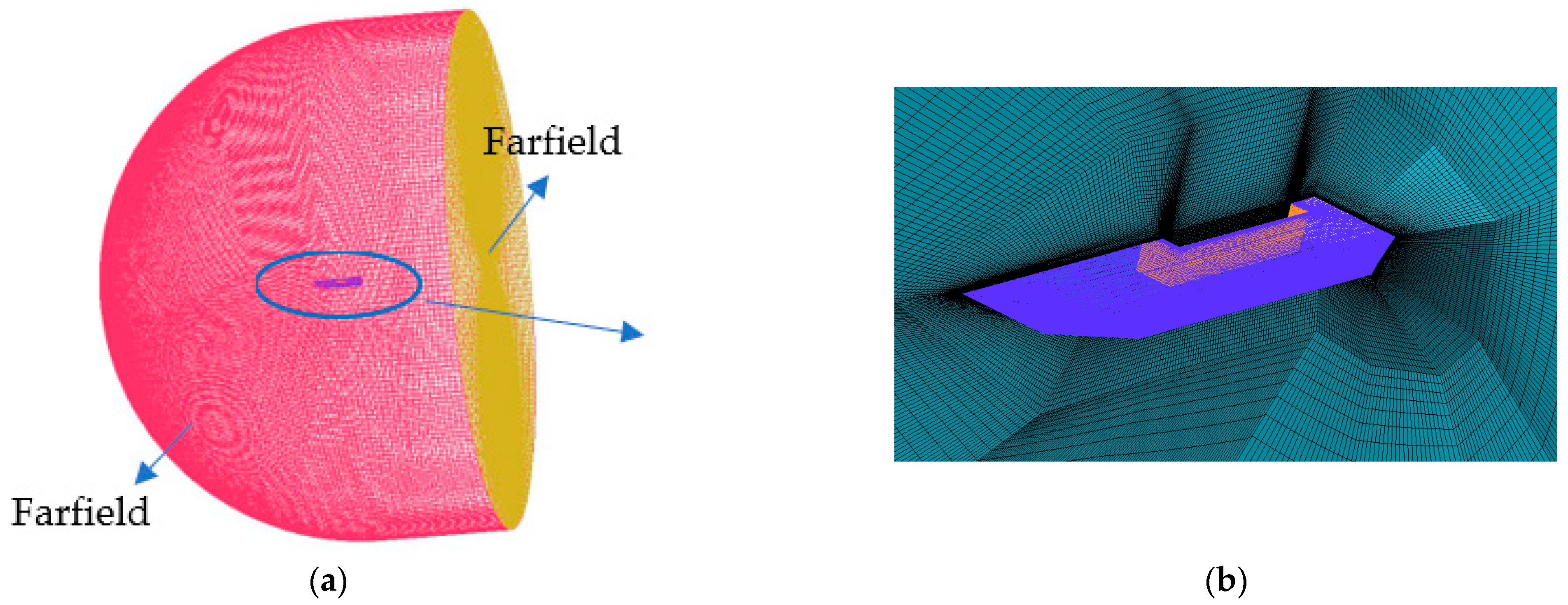
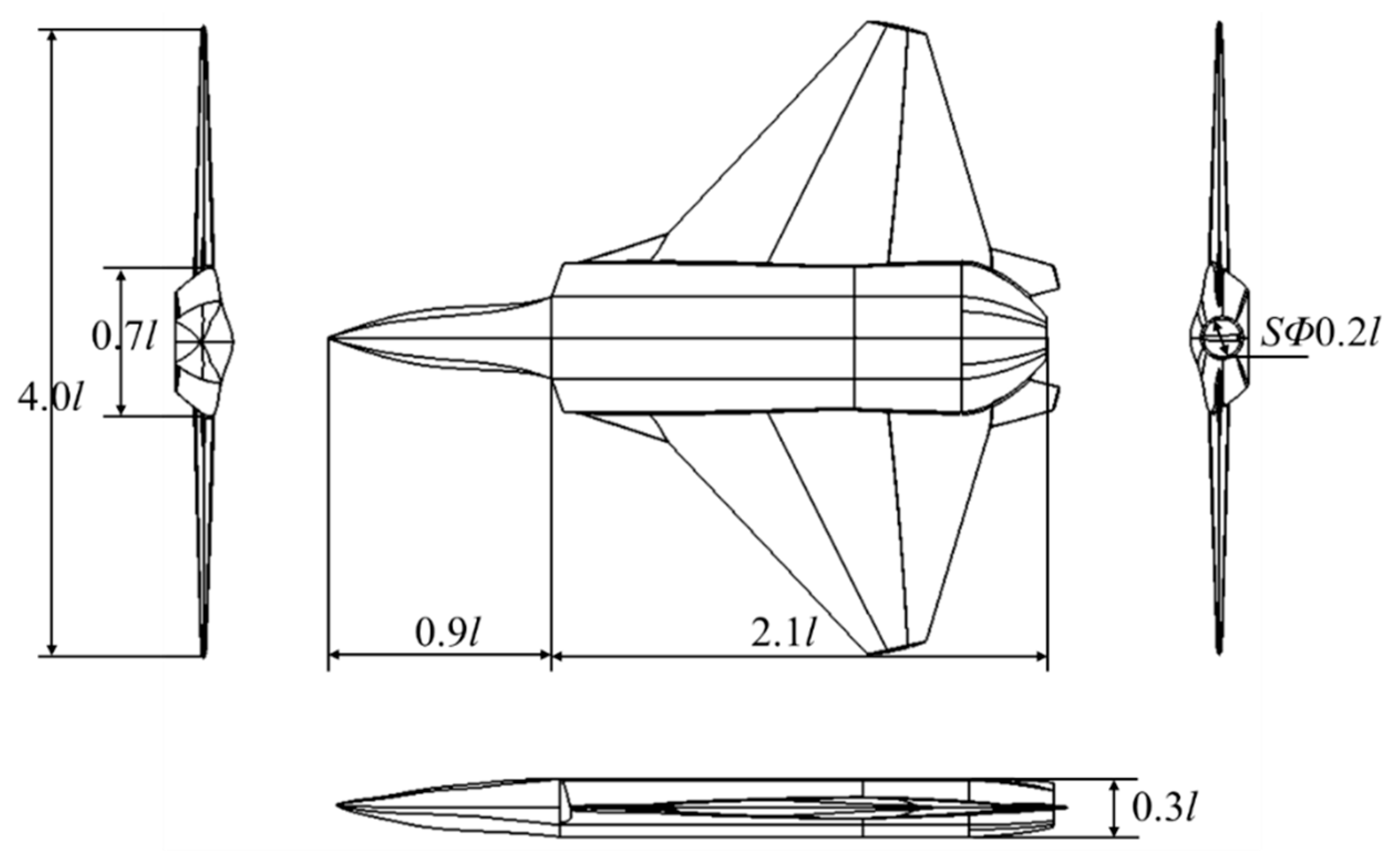
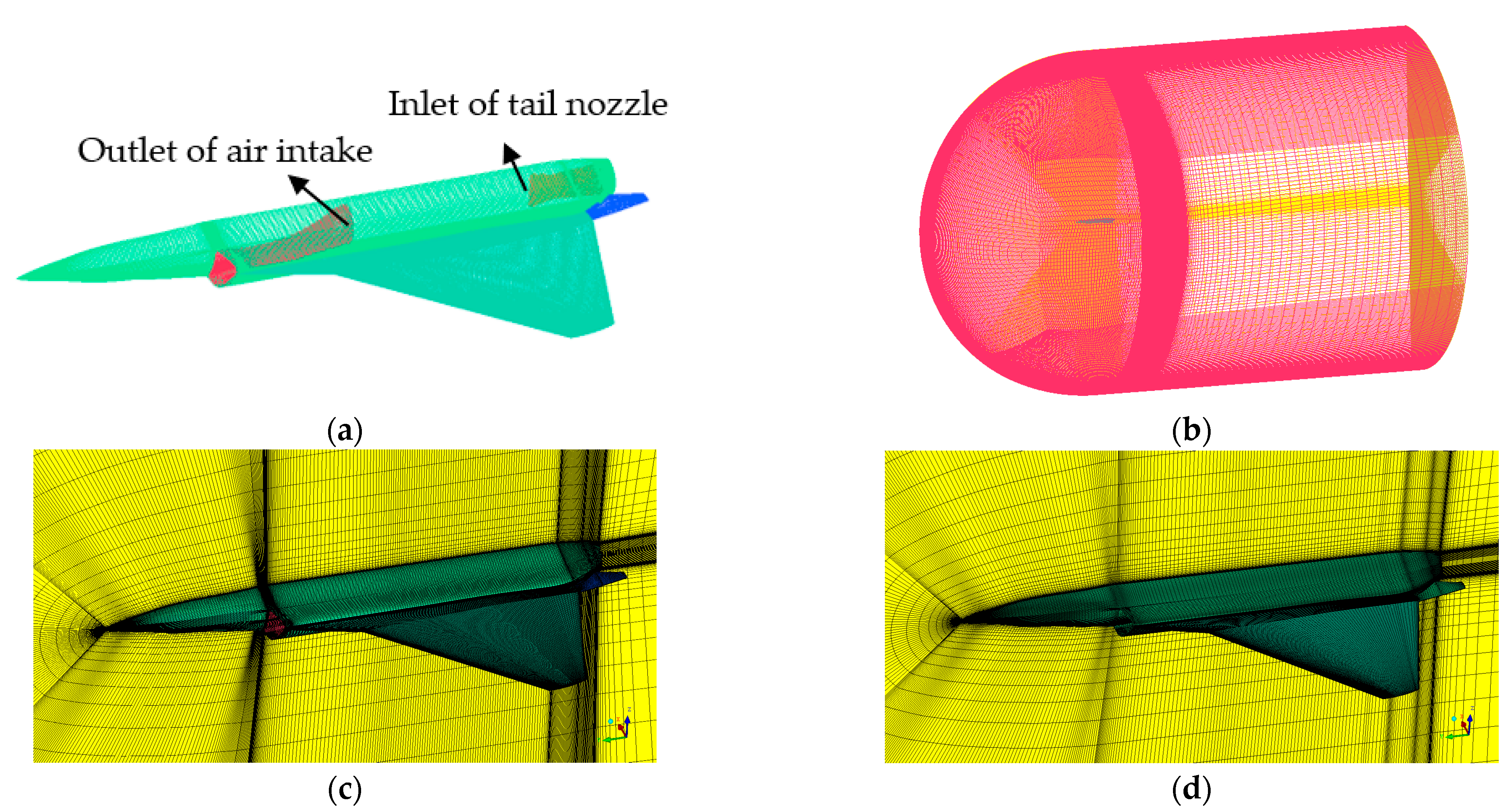
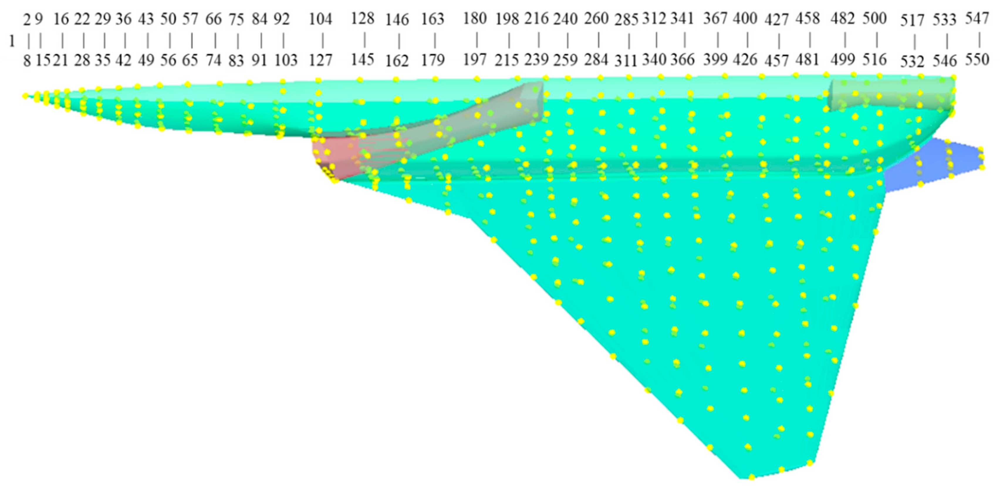
4.1. Geometry and Mesh Model

Considering a certain aircraft as the research object (as shown in Figure 9), this study established a geometric model of the aircraft, including the air intake and tail nozzle, and divided it into structured grids. The engine is a single-tail nozzle model with twin inlets, and the mesh model of the aircraft noise calculation is shown in Figure 10. The aircraft mesh model is shown in Figure 10a, and the computational domain mesh model is shown in Figure 10b. Using the NLAS method to calculate aircraft surface noise, the RANS mesh can be used to simulate the propagation of pressure pulsation, or the data can be interpolated on an independent acoustic mesh. By interpolating the RANS statistical data into a separate acoustic mesh, noise can be solved using more isotropic elements. Owing to the relaxation of the near-wall grid requirements, the y+ value can be much greater than one. Therefore, in the direction perpendicular to the wall, the fine boundary layer grid is no longer required, and the total number of grids and calculation time are significantly reduced, which is also an advantage of the NLAS method. Two sets of calculation meshes were used herein. Figure 10c shows the RANS mesh with 24.4 million elements, and Figure 10d shows the acoustic mesh with 9.1 million elements.
In the RANS calculation, the inflow Mach number was 1.6, the flight altitude was 11 km, and the angle of attack was 2.3°. The outlet of the air intake was the mass flow boundary condition, and the inlet of the nozzle was a characteristic-based boundary condition. According to the isentropic flow relation of aerodynamics, the mass flow rate at the outlet of the air intake was 42.59 kg/s. The static pressure and temperature at the nozzle inlet were 201,025 Pa and 1845.2 K, respectively, to simulate the air pressurisation process in an actual engine. The wall of the aircraft was non-slip. The cubic kε turbulence model was used for the calculation. After the statistical average values of the stress tensor and heat flux were obtained, they were interpolated into the acoustic mesh, and the turbulence was manually reconstructed according to the statistical average results. During the noise calculation, the unsteady calculation was started, the time step was 5 × 10⁻⁵ s, the flow solution time was 1.5 s, the maximum number of iterations in each time step was 10, and a new boundary was set as the absorption layer boundary. The monitoring points were set on the surface of the aircraft; the locations of the monitoring points are shown in Figure 11.

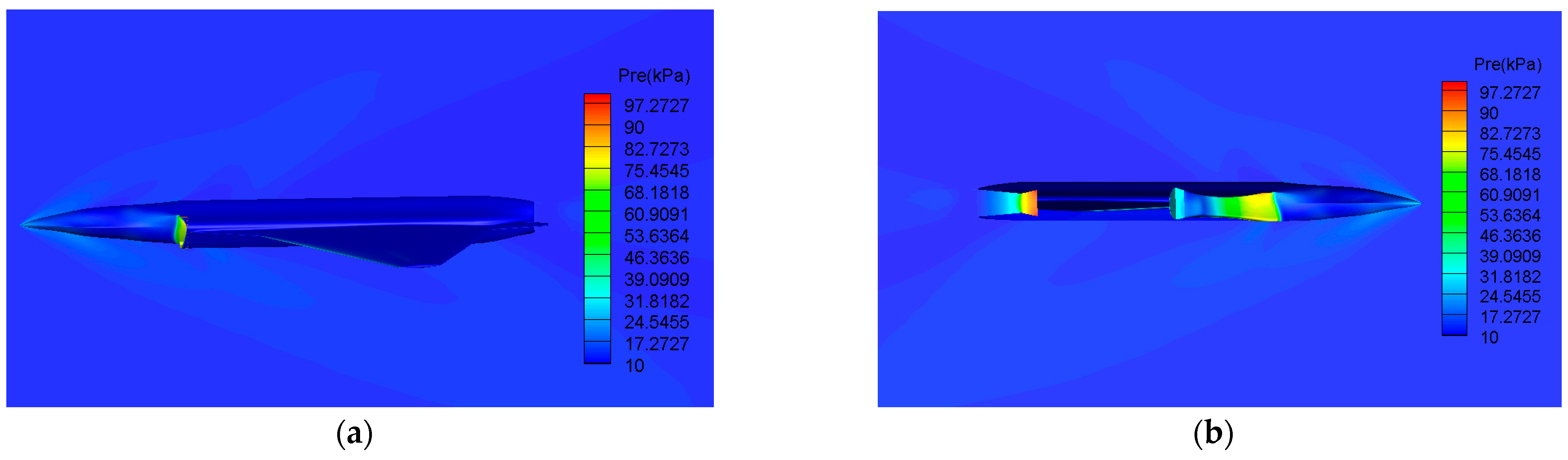
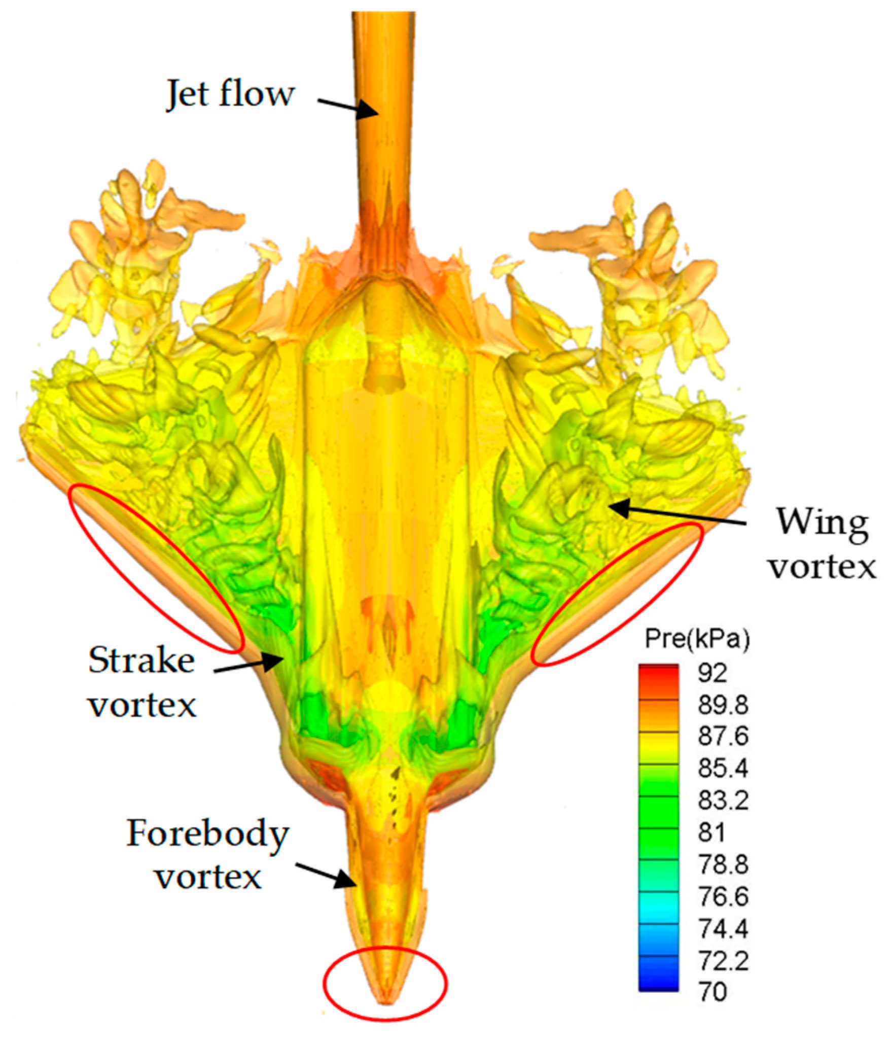
4.2. Numerical Results and Discussion

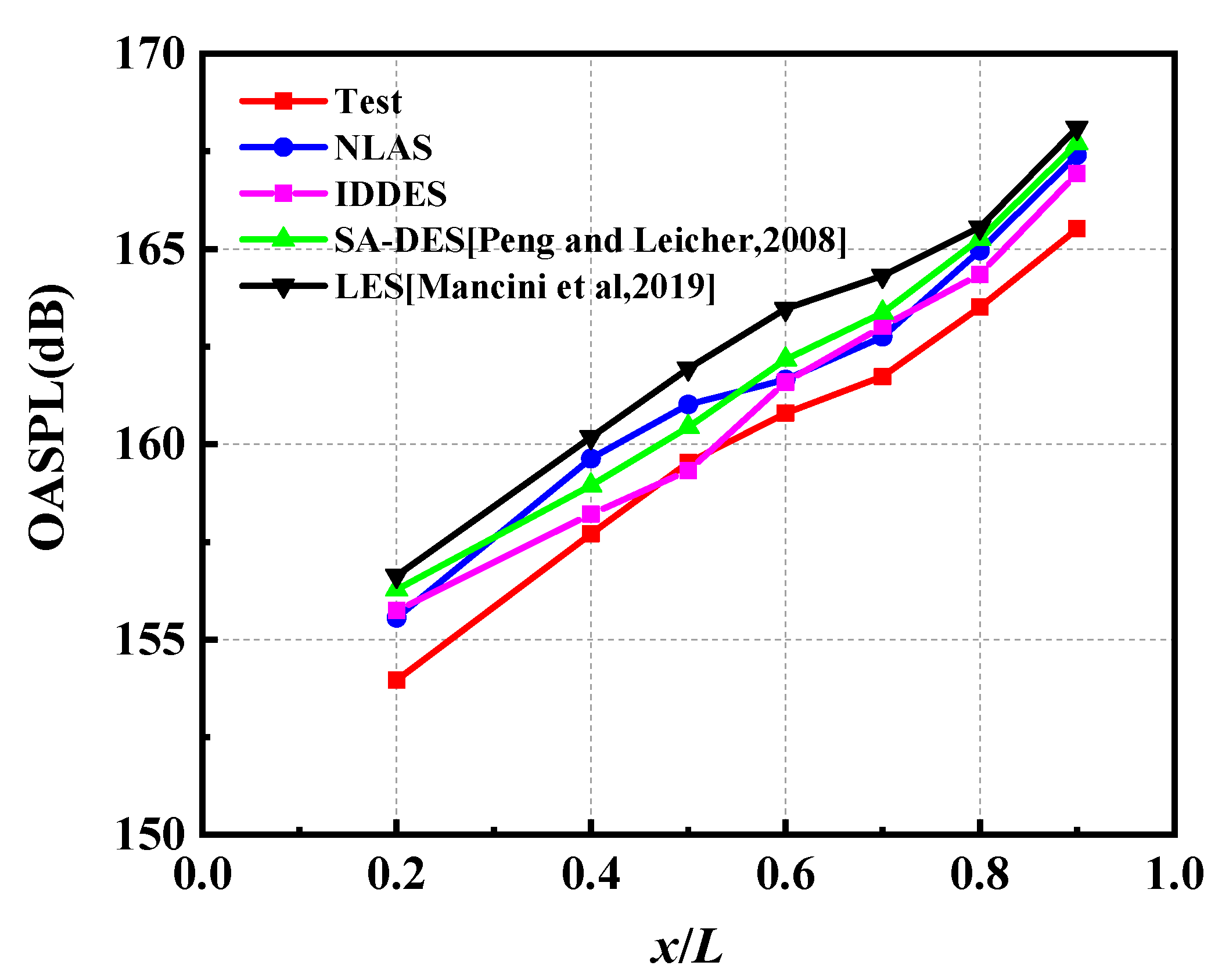
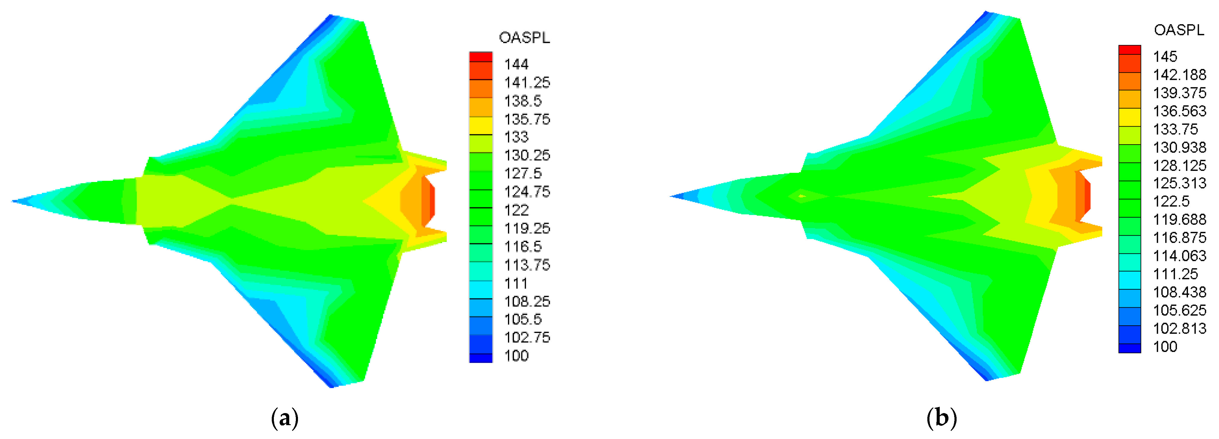
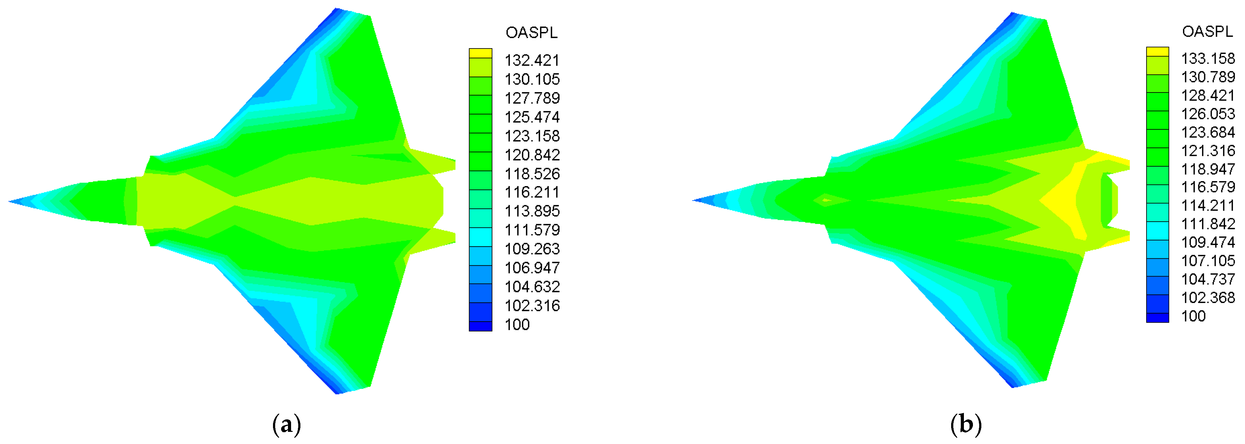
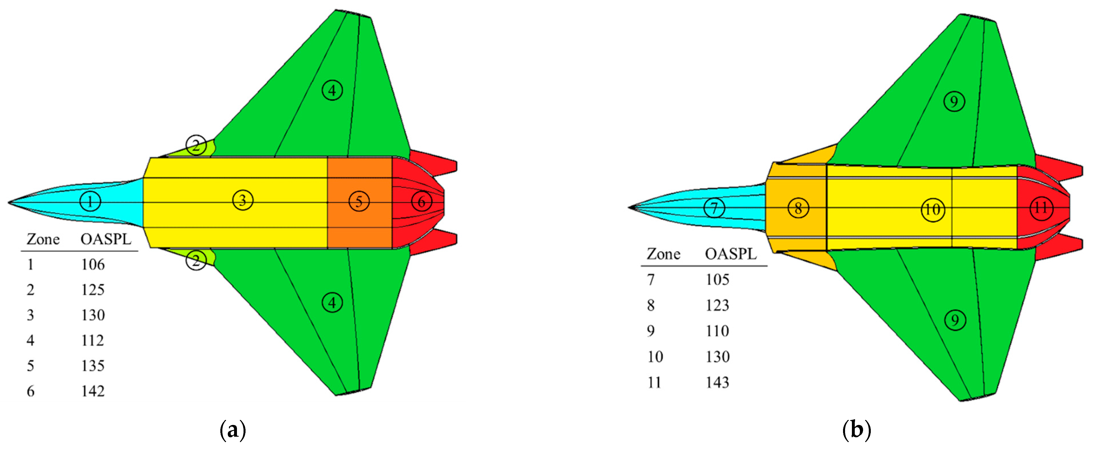
4.2.1. OASPL on Aircraft Surface

Figure 12 shows the pressure of the aircraft during supersonic flight. On the surface of the aircraft, the pressure at the nose and leading edge of the wing is high. Inside the fuselage, the pressure at the entrance of the air intake and the nozzle is high. The inlet of the air intake is greatly impacted by the pulsation of the airflow, and its characteristics need to be analysed later. The shock waves at the nose and tail can be seen in Figure 13: attachment shock wave at the nose and expansion wave at the tail.
The pressure fluctuation curves at the monitoring points can be obtained by calculations, and the sound pressure level spectrum curves at the monitoring points can be obtained by the Fourier transform. According to the formula:
OASPL = 10 lg f min f max 10 0.1 S P L f
The OASPL at each monitoring point can be calculated. Figure 14 is the cloud chart of the OASPL on the upper and lower surfaces of the aircraft made by the program. It can be observed from the figure that the OASPL at the nose and leading edge of the wing was relatively small and that the air intake and tail nozzle was relatively large. During the flight, the airflow on the aircraft surface gradually transitioned from attached to separated flow, the airflow pulsation increased, and the OASPL of the fuselage gradually increased from front to rear. Owing to the existence of supersonic jet noise at the tail nozzle, the OASPL was the largest, reaching 145 dB. Figure 15 is the cloud chart of the OASPL on the aircraft surface without jet noise. Compared with that with jet noise (Figure 14), the OASPL at the front of the fuselage was almost unchanged, the OASPL decreased only at the tail nozzle, and the maximum value became 133 dB. This shows that the surface aerodynamic noise is the main acoustic source when the aircraft is in a supersonic cruise state, and the jet noise has little effect on the sound pressure level at the front of the fuselage but only contributes to the OASPL at the tail nozzle of the fuselage. The intensity of pressure pulsations from the engine exhaust in the tail section is 93.3% of the total intensity of pressure pulsations.
Figure 16 shows the isosurface of the instantaneous Q = 300 criterion of the aircraft in cruise states. The isosurface’s instantaneous Q = 300, related to the vortex structure, was coloured by the absolute pressure. The Q isosurface can significantly express the vortex structure of the flow field. It can be seen that the forebody vortex bent outwards near the strake vortex along the front of the nose and finally met the strake vortex near the wing body fusion, which was also the location of vortex breakdown. After the vortex broke, it continued to move backward. Therefore, the pressure change on the upper surface of the fuselage was mainly caused by the change in the vortex structure. In actual flight, the vortex structure is helpful to increase the negative pressure on the upper surface of the fuselage and increase the lift. The aircraft in this study has no vertical tail, and the pitching balance and control are completed by the wing’s trailing edge aileron. There is no vertical tail buffeting problem, which further enhances the stealth and safety performance of the aircraft.
In Figure 16, the elliptical region is the nose and the leading edge of the wing. The region is subject to large pressure, but the turbulence fluctuation is small, so the sound pressure level in the elliptical region is small, as shown in Figure 14. Extract the pressure fluctuation curves of monitoring points 60, 268, and 520, as shown in Figure 17. It can be observed that the pressure of the fuselage decreases gradually from front to back along the fuselage, while the pulsating pressure ΔP increases gradually and the corresponding OASPL increases gradually. It can be seen that the SPL is independent of the pressure but relates to the pressure fluctuation.

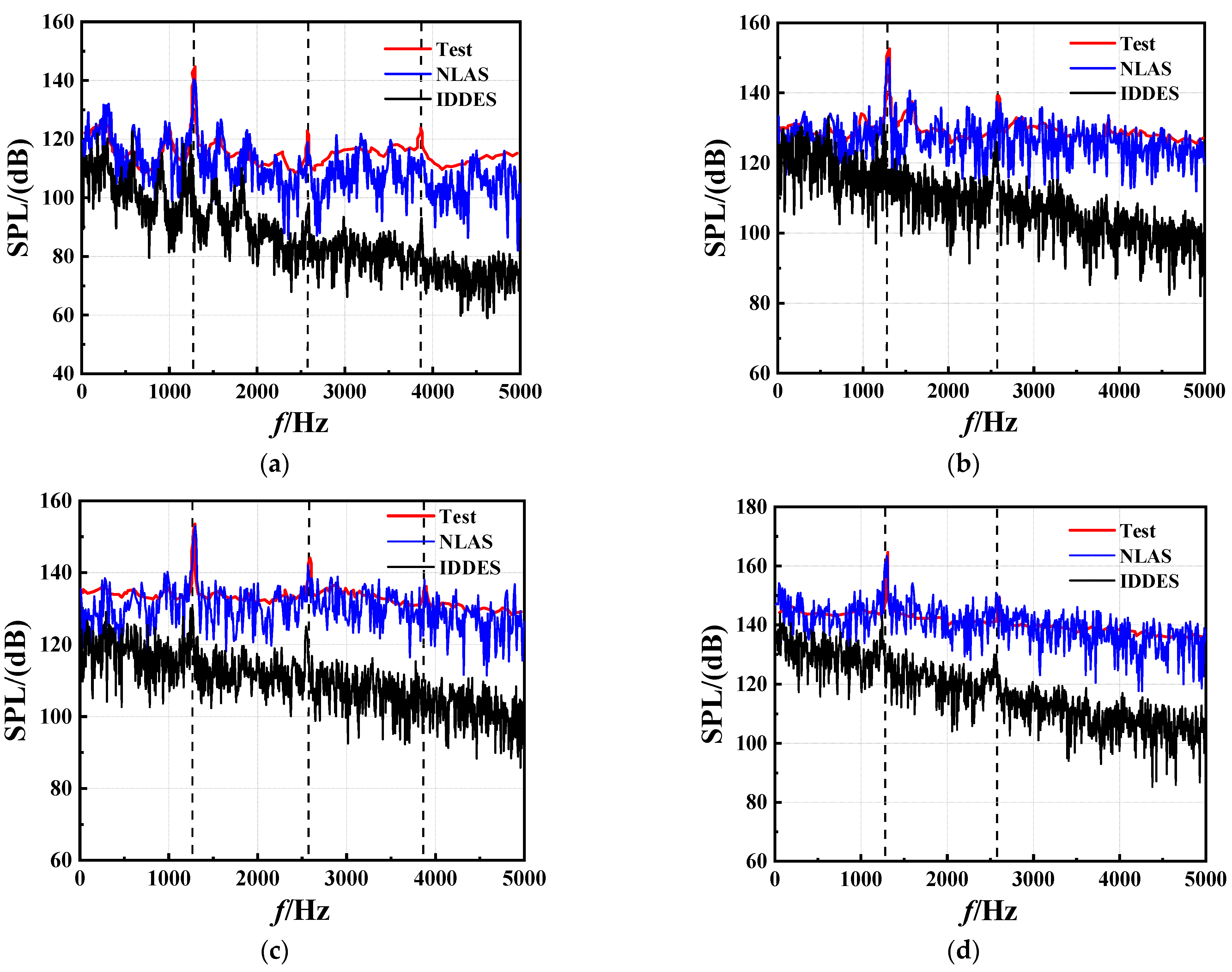
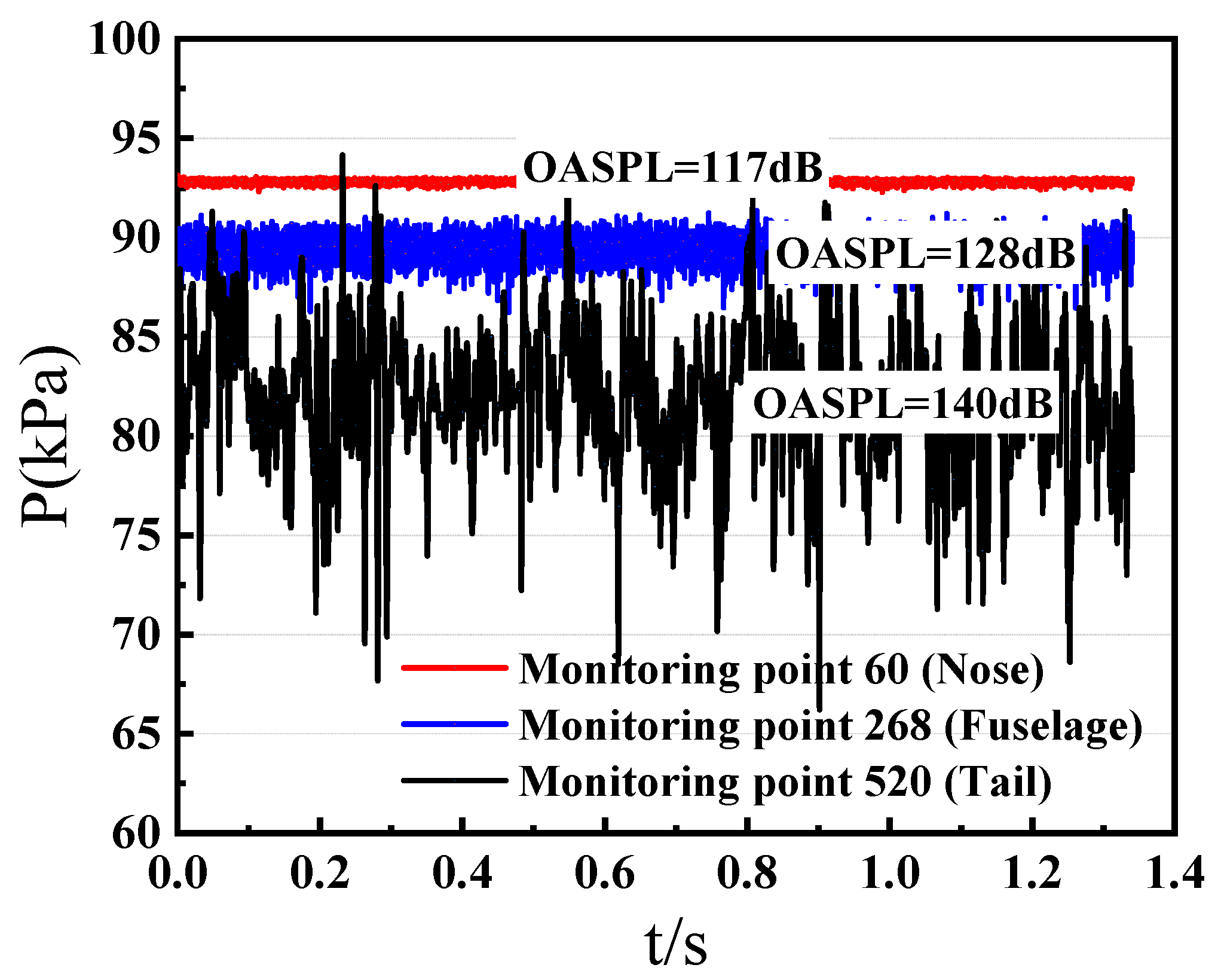
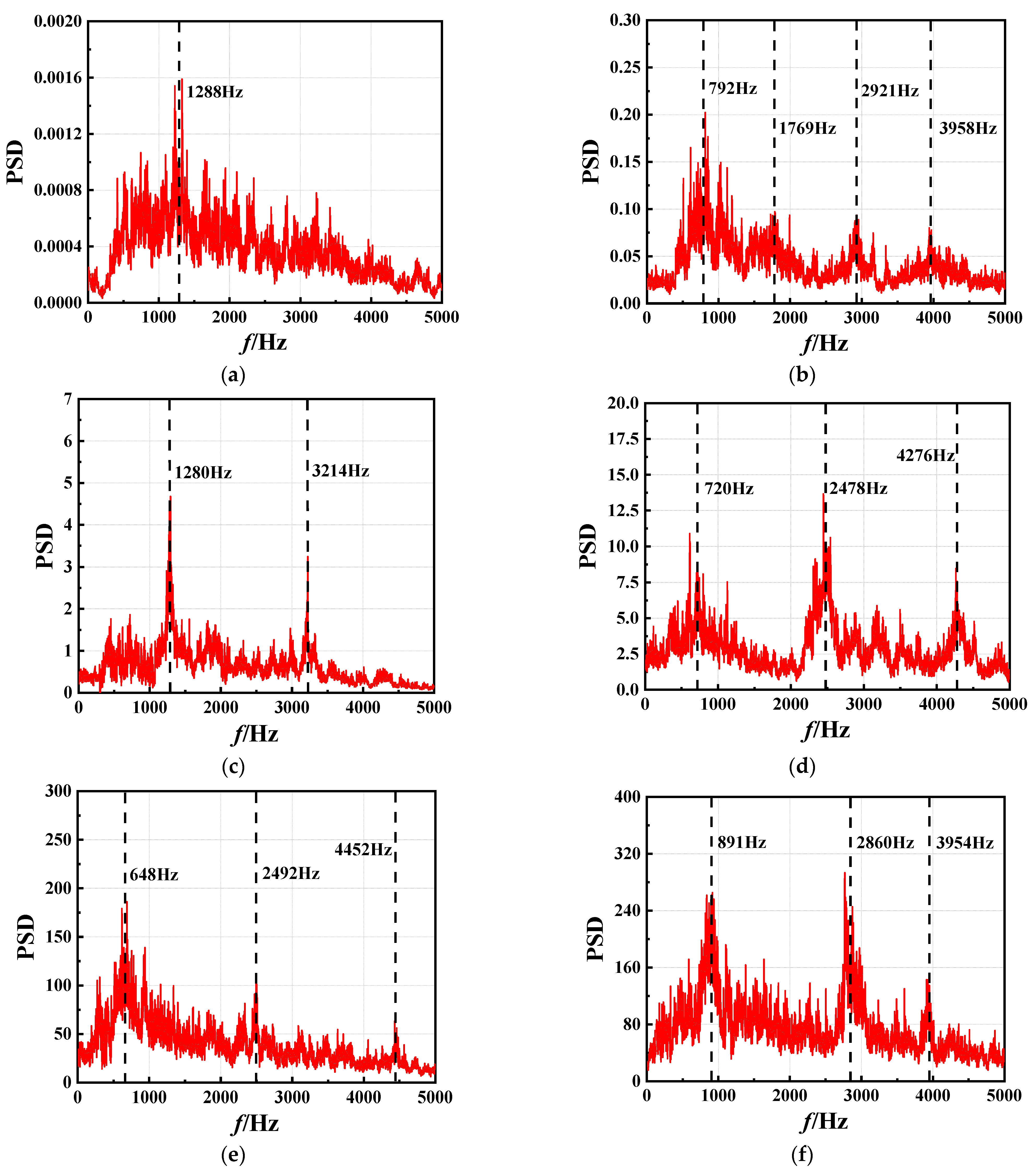
4.2.2. Power Spectral Density of Pressure Fluctuation

The pressure fluctuation power spectral density (PSD) of each monitoring point can be calculated using the NLAS method. The PSD of the monitoring points in the focus area is shown in Figure 18. Monitoring point 3 is located at the front of the nose. Compared with the other monitoring points, the PSD value of monitoring point 3 was very small. Although the front of the nose was subjected to a large aerodynamic pressure, the airflow pulsation was extremely small; therefore, the PSD value of the pressure pulsation was very small. As air flowed along the fuselage, the aircraft wall was accompanied by complex transitions and turbulence. The airflow produced complex flows such as separation, reattachment, and shock oscillation in the boundary layer. The PSD values of monitoring points 60, 200, and 520 on the fuselage surface gradually increased. From the PSD curve, it can be observed that the airflow pulsation energy on the aircraft surface was relatively evenly distributed over a wide frequency range. The PSD value of the airflow pulsation in the air intake (monitoring point 556) and tail nozzle (monitoring point 593) was relatively large, and the energy had a peak value in the low, medium, and high frequency ranges, which also reminded designers to check the strength of key components such as the air intake during aircraft design.

4.3. Calculation with Empirical Formulas

The following describes the process used to define external aero-acoustic loads using semi-empirical methods. The definition starts with a general vehicle arrangement. Features that may contribute to acoustic loads and determine appropriate empirical models for the region and flow conditions of interest were identified. The air intake, nozzle, leading edges, and surface bumps contributed to the loads. Semi-empirical models were applied to the flight trajectory, and critical acoustic design load conditions were determined for different types of flows, including the attached/turbulent boundary layer (A/TBL) and the separated/turbulent boundary layer (S/TBL). The CFD results were used to identify areas and conditions where turbulent, vortical, and/or shock-induced separated flow conditions existed. Semi-empirical methods were applied to determine acoustic levels and spectra based on the trajectory. Some of these semi-empirical methods are described in [39,40,41,42,43,44]. Finally, the vehicle was mapped into regions of similar flow types and levels, and all the load and design factors were applied. For this analysis, an acoustic model was used for different flow conditions [43]:
A / TBL OASPL = 16.153 × Ln M + 150 Alt × 0.0004 ,
S / TBL OASPL = 20 × Log q + 20 × Log 0.0078 / P ref + 20 × Log 1 + Ca / θ 0.5 ,
where M is the Mach number; Alt is the altitude in ft; Pref is the reference pressure, and it is 2.9 × 10⁻⁹ psi herein; q is the dynamic pressure in psf; Ca is the leading-edge cone angle; θ is the angle of attack.
Acoustic zone maps were developed based on streamlined acoustic load predictions, CFD analysis, and empirical models. Figure 19 shows maps of the upper and lower acoustic zones. Regions of similar flow types and acoustic levels are colour-coded. The acoustic levels were not specifically predicted for the exhaust region in this study, but approximate estimates of the acoustic levels were developed based on the effective nozzle area and exit flow velocity. The variation ranges of the OASPL on the aircraft surface calculated by the empirical formula are 105 dB~143 dB, and the overall distribution law is consistent with the simulation results. However, the empirical formula method can only calculate the OASPL in areas with similar flows. At present, there are few flow types in the empirical formulas that cannot accurately characterise the distribution of acoustic load on the aircraft surface.

5. Conclusions

The non-linear acoustics solver method avoids the additional dissipation of turbulent kinetic energy by artificially synthesising sub-grid-scale turbulence. At the same time, the NLAS method is based on the pulsation equations, which gives it a high accuracy in calculating supersonic aerodynamic noise.
In a supersonic cruise state, the external flow field of the aircraft and the internal flow field of the engine were solved simultaneously, followed by the internal and external acoustic fields, to obtain the distribution of the noise on the entire aircraft surface under the coupling acoustic sources. The PSD of the pressure pulsation in the key parts of the aircraft was analysed. The air intake and tail nozzle are subject to large low- and intermediate-frequency pulsations, so structural strength needs to be verified.
In a supersonic cruise state, the OASPL at the nose and leading edge of the wing are relatively small, and that at the air intake and tail nozzle is relatively large. The jet noise cannot propagate forward, and its contribution to aircraft surface noise is small; it only contributes to the OASPL at the tail nozzle of the fuselage. The intensity of pressure pulsations from the engine exhaust in the tail section is 93.3% of the total intensity of pressure pulsations. The research methods and results of this study can provide references for the development of new aircraft and the acoustic fatigue design of aircraft.

Author Contributions

Conceptualization, B.L.; methodology, H.D.; software, X.Z.; validation, X.Z.; formal analysis, X.Z.; investigation, H.D.; resources, B.L.; data curation, X.Z.; writing—original draft preparation, X.Z.; writing—review and editing, H.D. and B.L.; project administration, B.L.; funding acquisition, B.L. All authors have read and agreed to the published version of the manuscript.

Funding

This research was funded by the Innovation Foundation for Doctoral Dissertation of Northwestern Polytechnical University, grant number CX2022002. The National Natural Science Foundation of China, grant number 11872312, and the Natural Science Basic Research Plan in Shaanxi Province of China, grant number 2020JM-233.

Data Availability Statement

Sample data is available on request.

Acknowledgments

The authors thank the editor and reviewers for their valuable suggestions.

Conflicts of Interest

The authors declare no conflict of interest.

References

  1. Filippone, A. Aircraft noise prediction. Prog. Aerosp. Sci. 2014, 68, 27–63. [Google Scholar] [CrossRef]
  2. Li, Y.; Wang, X.; Zhang, D. Control strategies for aircraft airframe noise reduction. Chin. J. Aeronaut. 2013, 26, 249–260. [Google Scholar] [CrossRef]
  3. Thawre, M.; Pandey, K.; Dubey, A.; Verma, K.; Peshwe, D.; Paretkar, R.; Jagannathan, N.; Manjunatha, C. Fatigue life of a carbon fiber composite T-joint under a standard fighter aircraft spectrum load sequence. Compos. Struct. 2015, 127, 260–266. [Google Scholar] [CrossRef]
  4. Khorrami, M.; Lockard, D.; Humphreys, W.; Choudhari, M.; Van de Ven, T. Preliminary analysis of acoustic measurements from the NASA-Gulfstream airframe noise flight test. In Proceedings of the 14th AIAA/CEAS Aeroacoustics Conference (29th AIAA Aeroacoustics Conference), Vancouver, BC, Canada, 5–7 May 2008. [Google Scholar] [CrossRef]
  5. Stoker, R.; Gutierrez, R.; Larssen, J.; Underbrink, J.; Gatlin, G.; Spells, C. High Reynolds number aeroacoustics testing in NASA’s national transonic facility (NTF). In Proceedings of the 46th AIAA Aerospace Sciences Meeting and Exhibit, Reno, NV, USA, 7–10 January 2008; p. 838. [Google Scholar]
  6. Blacodon, D. Analysis of the Airframe Noise of an A320/A321 with a Parametric Method. J. Aircr. 2007, 44, 26–34. [Google Scholar] [CrossRef]
  7. Scarselli, G.; Amoroso, F.; Lecce, L.; Janssens, K.; Vecchio, A. Numerical simulation, experimental comparison with noise measurments and sound synthesis of airframe noise. In Proceedings of the 13th AIAA/CEAS Aeroacoustics Conference (28th AIAA Aeroacoustics Conference), Rome, Italy, 21–23 May 2007; p. 3460. [Google Scholar] [CrossRef]
  8. Sanders, M.P.J.; Koenjer, C.F.J.; Botero-Bolivar, L.; dos Santos, F.L.; Venner, C.H.; de Santana, L.D. Trailing-Edge Noise Comparability in Open, Closed, and Hybrid Wind Tunnel Test Sections. AIAA J. 2022, 60, 4053–4067. [Google Scholar] [CrossRef]
  9. Kuo, C.W.; Veltin, J.; McLaughlin, D.K. Acoustic measurements of models of military style supersonic nozzle jets. Chin. J. Aeronaut. 2014, 27, 23–33. [Google Scholar] [CrossRef]
  10. Chen, B.; Yang, X.; Chen, G.; Tang, X.; Ding, J.; Weng, P. Numerical study on the flow and noise control mechanism of wavy cylinder. Phys. Fluids 2022, 34, 036108. [Google Scholar] [CrossRef]
  11. Yu, P.; Peng, J.; Bai, J.; Han, X.; Song, X. Aeroacoustic and aerodynamic optimization of propeller blades. Chin. J. Aeronaut. 2020, 33, 826–839. [Google Scholar] [CrossRef]
  12. Liu, H.; Zhang, S.; Chen, R.; Zhou, S.; Zhao, Y. Numerical study on aerodynamic drag and noise of circular cylinders with a porous plate. Aerosp. Sci. Technol. 2022, 123, 107460. [Google Scholar] [CrossRef]
  13. Tao, J.; Sun, G. An artificial neural network approach for aerodynamic performance retention in airframe noise reduction design of a 3D swept wing model. Chin. J. Aeronaut. 2016, 29, 1213–1225. [Google Scholar] [CrossRef]
  14. Incheol, L.E.E.; Zhang, Y.; Dakai, L.I.N. A model-scale test on noise from single-stream nozzle exhaust geometries in static conditions. Chin. J. Aeronaut. 2018, 31, 2206–2220. [Google Scholar] [CrossRef]
  15. Bu, Y.; Song, W.; Han, Z.; Zhang, Y.; Zhang, L. Aerodynamic/aeroacoustic variable-fidelity optimization of helicopter rotor based on hierarchical Kriging model. Chin. J. Aeronaut. 2020, 33, 476–492. [Google Scholar] [CrossRef]
  16. Cavalieri, A.V.G.; Jordan, P.; Colonius, T.; Gervais, Y. Axisymmetric superdirectivity in subsonic jets. J. Fluid Mech. 2012, 704, 388–420. [Google Scholar] [CrossRef]
  17. Reba, R.; Narayanan, S.; Colonius, T. Wave-packet models for large-scale mixing noise. Int. J. Aeroacoust. 2010, 9, 533–557. [Google Scholar] [CrossRef]
  18. Abalakin, I.; Dervieux, A.; Kozubskaya, T. High accuracy finite volume method for solving nonlinear aeroacoustics problems on unstructured meshes. Chin. J. Aeronaut. 2006, 19, 97–104. [Google Scholar] [CrossRef]
  19. Legendre, C.; Ficat-Andrieu, V.; Poulos, A.; Kitano, Y.; Nakashima, Y.; Kobayashi, W.; Minorikawa, G. A machine learning-based methodology for computational aeroacoustics predictions of multi-propeller drones. In Proceedings of the INTER-NOISE and NOISE-CON Congress and Conference Proceedings, Washington, DC, USA, 11–13 August 2021; Institute of Noise Control Engineering: Reston, VA, USA; Volume 263, pp. 3467–3478. [Google Scholar]
  20. Pham, N.K.; Nguyen, P.K.; Duong, N.T. Computational Simulation of Aerodynamic Noise Generation on High-Lift Configuration. J. Aeronaut. Astronaut. Aviat. 2022, 54, 393–403. [Google Scholar] [CrossRef]
  21. Lockard, D.; Choudhari, M. Noise radiation from a leading-edge slat. In Proceedings of the 15th AIAA/CEAS Aeroacoustics Conference (30th AIAA Aeroacoustics Conference), Miami, FL, USA, 11–13 May 2009; p. 3101. [Google Scholar] [CrossRef]
  22. König, D.; Koh, S.; Schröder, W.; Meinke, M. Slat noise source identification. In Proceedings of the 15th AIAA/CEAS Aeroacoustics Conference (30th AIAA Aeroacoustics Conference), Miami, FL, USA, 11–13 May 2009; p. 3100. [Google Scholar] [CrossRef]
  23. Ricciardi, T.R.; Wolf, W.R.; Moffitt, N.J.; Kreitzman, J.R.; Bent, P. Numerical noise prediction and source identification of a realistic landing gear. J. Sound Vib. 2021, 496, 115933. [Google Scholar] [CrossRef]
  24. Redonnet, S.; Ben Khelil, S.; Bulté, J.; Cunha, G. Numerical characterization of landing gear aeroacoustics using advanced simulation and analysis techniques. J. Sound Vib. 2017, 403, 214–233. [Google Scholar] [CrossRef]
  25. Prasad, C.; Hromisin, S. Coupled LES-experimental noise source imaging and fluid-thermodynamic mode decomposition of supersonic jets with fluid inserts. In Proceedings of the AIAA Scitech 2020 Forum, Orlando, FL, USA, 6–10 January 2020; p. 1000. [Google Scholar]
  26. Shen, W.; Patel, T.K.; Miller, S.A. Extraction of large-scale coherent structures from large eddy simulation of supersonic jets for shock-associated noise prediction. In Proceedings of the AIAA Scitech 2020 Forum, Orlando, FL, USA, 6–10 January 2020; p. 0742. [Google Scholar]
  27. Yen, J.; Kimbrell, A.; Connor, C. Study of WICS data using an emerging lower-order CAA method. In Proceedings of the US Air Force T&E Days 2010, Nashville, TN, USA, 2–4 February 2010; p. 1742. [Google Scholar] [CrossRef]
  28. Rodriquez, G.; Velez, C.; Ilie, M. Numerical studies of high-speed cavity flows using LES, DDES and IDDES. In Proceedings of the 51st AIAA Aerospace Sciences Meeting, Grapevine, TX, USA, 7–10 January 2013. [Google Scholar]
  29. André, B.; Castelain, T.; Bailly, C. Shock oscillations in a supersonic jet exhibiting antisymmetrical screech. AIAA J. 2012, 50, 2017–2020. [Google Scholar] [CrossRef]
  30. Yao, C.; Zhang, G.H.; Liu, Z.S. Forced shock oscillation control in supersonic intake using fluid–structure interaction. AIAA J. 2017, 55, 2580–2596. [Google Scholar] [CrossRef]
  31. Batten, P.; Ribaldone, E.; Casella, M.; Chakravarthy, S. Towards a generalized non-Linear acoustics solver. In Proceedings of the 10th AIAA/CEAS Aeroacoustics Conference, Manchester, UK, 10–12 May 2004. [Google Scholar] [CrossRef]
  32. Kraichnan, R.H. Diffusion by a random velocity field. Phys. Fluids 1969, 13, 22–31. [Google Scholar] [CrossRef]
  33. Smirnov, A.; Shi, S.; Celik, I. Random flow generation technique for large eddy simulations and particle-dynamics modeling. J. Fluid. Engin. 2001, 123, 359–371. [Google Scholar] [CrossRef]
  34. Batten, P.; Goldberg, U.; Chakravarthy, S. Reconstructed sub-grid methods for acoustics predictions at all Reynolds numbers. In Proceedings of the 8th AIAA/CEAS Aeroacoustics Conference, Breckenridge, CO, USA, 17–19 June 2002. [Google Scholar] [CrossRef]
  35. Henshaw, M.J. M219 cavity case. In Verification and Validation Data for Computational Unsteady Aerodynamics; Techology Report RTO-TR-26, AC/323(AVT)TP/19; QinetiQ: Farnborough, UK, 2002; pp. 453–472. [Google Scholar]
  36. Peng, S.H.; Leicher, S. DES and Hybrid RANS-LES Modelling of Unsteady Pressure Oscillations and Flow Features in a Rectangular Cavity. Advances in Hybrid RANS-LES Modelling; Springer: Berlin/Heidelberg, Germany, 2008; pp. 132–141. [Google Scholar]
  37. Mancini, S.; Kolb, A.; Gonzalez-Martino, I.; Casalino, D. Very-large eddy simulations of the m219 cavity at high-subsonic and supersonic conditions. In Proceedings of the AIAA Scitech 2019 Forum, San Diego, CA, USA, 5–7 January 2019; p. 1833. [Google Scholar] [CrossRef]
  38. Bridges, J.; Brown, C. Validation of the small hot jet acoustic rig for aeroacoustic research. In Proceedings of the 11th AIAA/CEAS Aeroacoustics Conference, Monterey, CA, USA, 23–25 May 2005; p. 2846. [Google Scholar] [CrossRef]
  39. Ungar, E.E.; Wilby, J.F.; Bliss, D.B.; Pinkel, B.; Galaitsis, A. A Guide for Estimation of Aeroacoustic Loads on Flight Vehicle Surfaces; Bolt Beranek and Newman Inc.: Cambridge, MA, USA, 1977. [Google Scholar]
  40. Coe, C.F.; Chyu, W.J. Pressure-Fluctuation Inputs and Response of Panels Underlying Attached and Separated Supersonic Turbulent Boundary Layers; NASA-TM-X-62189; NASA: Washington, DC, USA, 1972.
  41. Lowson, M.V. Prediction of Boundary Layer Pressure Fluctuations; Wyle Labs Inc.: Huntsville, AL, USA, 1968. [Google Scholar]
  42. Lew, H.G.; Laganelli, A.L. Fluctuating Pressure Loads for Hypersonic Vehicle Structures. Phase 1; Techquest Inc.: Huntsville, AL, USA, 1991. [Google Scholar]
  43. Laganelli, A.L. Prediction of the Pressure Fluctuations Associated with Maneuvering Reentry Weapons; Flight Dynamics Laboratory, Air Force Wright Aeronautical Laboratories, United States Air Force: Dayton, OH, USA, 1984.
  44. Wiley, D.R.; Seidl, M.G. Aerodynamic Noise Tests on X-20 Scale Models. Volume 2. Summary and Analysis Report; Boeing Aerospace Co.: Seattle, WA, USA, 1965. [Google Scholar]
Figure 1. (a) Cavity experimental model; (b) Position of sensors.
Aerospace 10 00439 g001
Figure 2. Cavity simulation mesh model: (a) Computational domain mesh; (b) Section of the cavity structured grid.
Aerospace 10 00439 g002
Figure 3. Comparison between the numerical simulation results and test results at Ma = 0.85 [36,37].
Aerospace 10 00439 g003
Figure 4. Comparison between the numerical simulation results and test results at Ma = 3.0: (a) Monitoring point 1; (b) Monitoring point 7; (c) Monitoring point 10; (d) Monitoring point 13.
Aerospace 10 00439 g004
Figure 5. Mesh model of the nozzle computational domain and boundary conditions.
Aerospace 10 00439 g005
Figure 6. Experimental device [38].
Aerospace 10 00439 g006
Figure 7. Axial velocity field.
Aerospace 10 00439 g007
Figure 8. Experiment and simulation data for the ARN2 nozzle at the 90° (top) and 150° (bottom) microphone locations. The data is scaled to a distance of 40 × (jet diameter) in a lossless condition: (a) 90°; (b) 150°.
Aerospace 10 00439 g008
Figure 9. Aircraft geometric model.
Aerospace 10 00439 g009
Figure 10. Computational mesh model: (a) Aircraft mesh model; (b) Computational domain mesh model; (c) RANS mesh; (d) Acoustic mesh.
Aerospace 10 00439 g010
Figure 11. Monitoring points on the aircraft surface.
Aerospace 10 00439 g011
Figure 12. Pressure of aircraft in supersonic flight: (a) Fuselage surface; (b) Fuselage interior.
Aerospace 10 00439 g012
Figure 13. Shock waves on the fuselage: (a) Fuselage surface; (b) Fuselage interior.
Aerospace 10 00439 g013
Figure 14. OASPL on aircraft surfaces: (a) Upper surface; (b) Lower surface.
Aerospace 10 00439 g014
Figure 15. OASPL on aircraft surfaces without jet noise: (a) Upper surface; (b) Lower surface.
Aerospace 10 00439 g015
Figure 16. The criterion of the isosurface of instantaneous Q = 300 is coloured by the local pressure and the distribution of pressure on the surface in motion.
Aerospace 10 00439 g016
Figure 17. Pressure pulsation of the monitoring points.
Aerospace 10 00439 g017
Figure 18. Power spectral density of pressure fluctuation at monitoring points: (a) Monitoring point 3; (b) Monitoring point 60; (c) Monitoring point 200; (d) Monitoring point 520; (e) Monitoring point 556; (f) Monitoring point 593.
Aerospace 10 00439 g018
Figure 19. The OASPL on the surface of aircraft is calculated by empirical formulas: (a) Upper surface; (b) Lower surface.
Aerospace 10 00439 g019
Table 1. Relative position of sensors.
PointLongitudinal x/LVertical y/D
10.2
20.4
30.5
40.6
50.7
60.8
70.9
8 0.143
9 0.286
10 0.429
11 0.571
12 0.714
13 0.857
Table 2. Efficiency (at Ma = 3.0), advantages, and disadvantages of different calculation methods.
Number of CPU CoresTime StepNumber of Grid CellsCalculation TimeAdvantagesDisadvantages
IDDES642.5 × 10−6 s7.5 million25 daysHigh accuracy of subsonic calculation. Unsteady state conditions can be calculated.Low accuracy of supersonic calculation. Low efficiency.
NLAS645 × 10−6 s3.2 million6 daysHigh accuracy of subsonic and supersonic calculations. High efficiency, suitable for engineering applications.Calculating based on the RANS equation and dynamic unsteady conditions cannot be done.
Disclaimer/Publisher’s Note: The statements, opinions and data contained in all publications are solely those of the individual author(s) and contributor(s) and not of MDPI and/or the editor(s). MDPI and/or the editor(s) disclaim responsibility for any injury to people or property resulting from any ideas, methods, instructions or products referred to in the content.

