Article

In-Plane Libration Suppression of a Two-Segment Tethered Towing System

State Key Laboratory of Mechanics and Control for Aerospace Structures, Nanjing University of Aeronautics and Astronautics, Nanjing 210016, China
*
Author to whom correspondence should be addressed.
Aerospace 2023, 10(3), 286; https://doi.org/10.3390/aerospace10030286
Submission received: 8 February 2023 / Revised: 8 March 2023 / Accepted: 9 March 2023 / Published: 13 March 2023
(This article belongs to the Special Issue Advanced Motion Planning and Control in Aerospace Applications)

Abstract

:
A tethered towing system provides an effective method for capturing pieces of space debris and dragging them out of orbit. This paper focuses on the in-plane stability analysis and libration control of a two-segment tethered towing system. The first segment is the same as the traditional single-tether towing system. The second segment is similar to a simplified space tether net. The dynamic equations are established in the orbit frame. Considering the elasticity of the tethers, the equilibrium solutions are obtained and the stability of equilibrium solutions is proved. An in-plane libration controller based on the sliding mode control scheme is designed to ensure the safety of the towing mission and save fuel. The controller suppressed the librations of the in-plane angles in the desired state by applying two external torques. Finally, simulation results are provided to validate the effectiveness of the proposed controller.

1. Introduction

According to European Space Agency (ESA)’s Space Environment Report 2022, more than 30,000 pieces of space debris have been spotted so far. Active debris removal technology becomes particularly necessary to ensure the safety of human assets in orbit [1]. Scholars have proposed dozens of schemes for removing debris. The use of a space net is an effective technique to remove debris. This method stabilizes the attitude of the captured debris by limiting its degrees of freedom [2]. Botta evaluated the effect of different mechanical models on the simulation of capturing the target using a net from the perspective of dynamic calculation [3]. Simulations have been performed to study target capturing using a space net [4,5]. Sharf et al. presented a space net closing mechanism. Experiments demonstrated the practicality of the net closing system [6]. Yue established the dynamic model of a rectangular space net and validated its accuracy by comparing it with on-ground experiments [7]. For active debris removal technology, Lv et al. proposed an integrated platform scheme [8].
A tethered towing system (TTS) is an active space debris removal technology derived from the tethered satellite system (TSS). TTS has become another one of the most likely solutions to the large debris deorbit due to its simple structure, light weight, low cost, variable system structural parameters, and large capture distance [9]. Stadnyk proposed a new tether model using s spring-damper element to simulate the target capture process [10]. Many studies have been carried out on the system dynamic analysis [11,12]. Abouelmagd studied the dynamic problem considering the effect of the zonal harmonic parameter [13]. Pang et al. studied the nonlinear dynamics of a TSS in the orbital plane and obtained the analytical solutions of internal resonance [14]. Aslanov and Ledkov studied the dynamic influence of the atmosphere on a TTS [15]. Later, Aslanov and Yudintsev studied the coupling dynamics between tether vibration and flexible attachment vibration when a TTS towed space debris with flexible attachments [16]. Then, they took the target with fuel residue as the research object and studied the influence of attitude motion of such objects on the safety of the towing process [17]. Aslanov et al. analyzed the balanced configuration and stability of the system and proposed guidelines for selecting appropriate thrust, tug mass, and tether length to avoid chaotic motion [18]. Aslanov and Yudintsev found that if the tether was connected off-center to the debris, shifting the orbit by changing the thrust would increase the pitch oscillations of the tether, ultimately leading to the chaotic motion of the system [19]. Aslanov also studied the stability of pendulum systems with moving mass blocks near the equilibrium position [20]. By considering the large deformation of a tether, Lim calculated the dynamic responses of a TTS for the variations of the capture angles and capture velocities of the debris, and the effects of varying system parameters were analyzed [21]. Shan performed modal analysis for a TTS and derived an analytical solution of the system’s natural frequency. The influence of the initial angular velocity of the target on the chaser satellite was analyzed [22].
Regarding the tether structures, Qi proposed a double-tether TTS, in which the tethers were connected to the edge of the debris [23]. Hovell proposed a bifurcated TTS and studied the system stability when capturing a non-cooperative failed spacecraft in the orbital environment [24,25,26]. Then the planar experiments were carried out. The results showed that the proposed system better exploited tether damping and improved despinning performance as compared to the single-tether configuration [27]. Yang et al. proposed a sub-tether configuration of a TTS and performed some simulations to demonstrate the effectiveness of the proposed system [28]. Shan compared the single-tether configuration and the sub-tether configuration based on three models, namely the modified dumbbell model, the lumped-mass model, and the ANCF model [22]. The sub-tether configuration provides a new way for active debris removal technology, which acquires the advantages of the space net and the TTS. However, it may exhibit more different dynamics behavior than the traditional single-tether configuration.
In terms of stability analysis, Abouelmagd et al. studied the positions of the equilibria points and their stability for a dumbbell satellite when the central body is an oblate spheroid [29]. Qi studied the equilibrium solutions and their stability for a TTS and proposed two feedback control schemes to stabilize the debris attitude [23]. Considering the debris as a flexible beam, Hu found that the mass ratio between the tug and the debris determines the equilibrium solutions and the reach time [30]. Lian et al. studied the chaotic motion and control problems using Melnikov’s method and proposed a chaotic control method based on an inertia damper [31]. Liu found that by increasing tether damping, the system motion could be stabilized near the equilibrium points and the quasi-periodic motion could be changed into periodic motion [32]. Sun and Zhao found that the mass of the main satellite had a significant influence on the stability and libration characteristics [33].
In terms of system control, Jin and Hu converted the optimal control problem into a linear programming problem by truncating the Chebyshev series and using the quasi-linearization method [34]. For the variable mass of the satellite, Sun et al. proposed a thrust control law using double-switching-type constant thrust [35]. Wen et al. proposed a tension control law based on potential energy shaping and damping injection with only the feedback of the tether length [36]. Zhang et al. designed an algorithm to stabilize TTS with a rotating target by controlling the position of the tug and the tether tension [37]. In order to enhance the robustness of the system, Yang et al. established a three-dimensional dynamic model. When the failed spacecraft had an initial angular velocity, the system could be stabilized by the tether connection point bias control method and tether length control [38]. Kang et al. proposed three control strategies to control a rotating uncooperative target with bounded stability. The effectiveness was validated experimentally using a microgravity platform with two tethered free-floating air-bearing satellite simulators [39].
Sliding mode control, which can overcome uncertainty and has strong robustness to interference, is especially suitable for nonlinear systems, and TTS is a typical nonlinear system. Razzaghi applied an adaptive sliding mode and the state-dependent Riccati equation control method on a TSS [40]. Chu added a time-varying control tension using a hierarchical sliding mode controller to implement the hybrid control of the in-plane angle and the relative distance [41]. Xu et al. developed a novel fractional-order fuzzy sliding mode control strategy and derived a fuzzy control law in analytical form, which could perform a faster and smoother deployment [42,43]. Kang et al. proposed a fractional order sliding mode control for the deployment, which consisted of two sub-sliding manifolds that were defined separately for the actuated and unactuated states [44]. Li presented a novel discrete-time pure-tension sliding mode predictive control scheme, which inherited the property of explicitly handling constraints from model predictive control and the remarkable robustness of sliding mode control [45]. Li developed a novel fractional-order nonsingular terminal sliding mode control scheme to stabilize an underactuated deployment mission with only tension regulation [46]. Then he investigated a super-twisting sliding mode controller to accelerate the convergence speed of system states and an adaptive law to handle the adverse effect of uncertainty and external disturbance [47]. Liu proposed a robust adaptive control strategy to solve the problem of attitude tracking control for a clean platform, and this control strategy is based on the coupling of the fuzzy logic system with sliding mode control [48]. Researchers have designed many sliding mode control schemes to realize the deployment of TSSs. However, works about suppressing a TTS’s in-plane libration are few.
This paper aims to solve the equilibrium configurations of a two-segment tethered towing system and design a controller to suppress the librations of in-plane angles by referring to previous studies. In contrast with the available literature, the contributions of the paper are as follows:
(1)
With the elasticity of the tethers, the equilibrium configurations of a two-segment tethered towing system with constant thrust are obtained and the stabilities of equilibria are proved.
(2)
An in-plane sliding mode controller is designed to suppress the librations of the in-plane angles of the system.
The rest of the paper is organized as follows: Section 2 describes the system composition and gives the dynamic formulations. In Section 3, the three-dimensional dynamic equations are simplified, and the equilibria and stability of the simplified model are studied. In Section 4, a libration controller is designed with the equilibrium solutions as the desired state. In Section 5, the system dynamic characteristics and the effectiveness of the designed controller are simulated. Conclusions are drawn in Section 6.

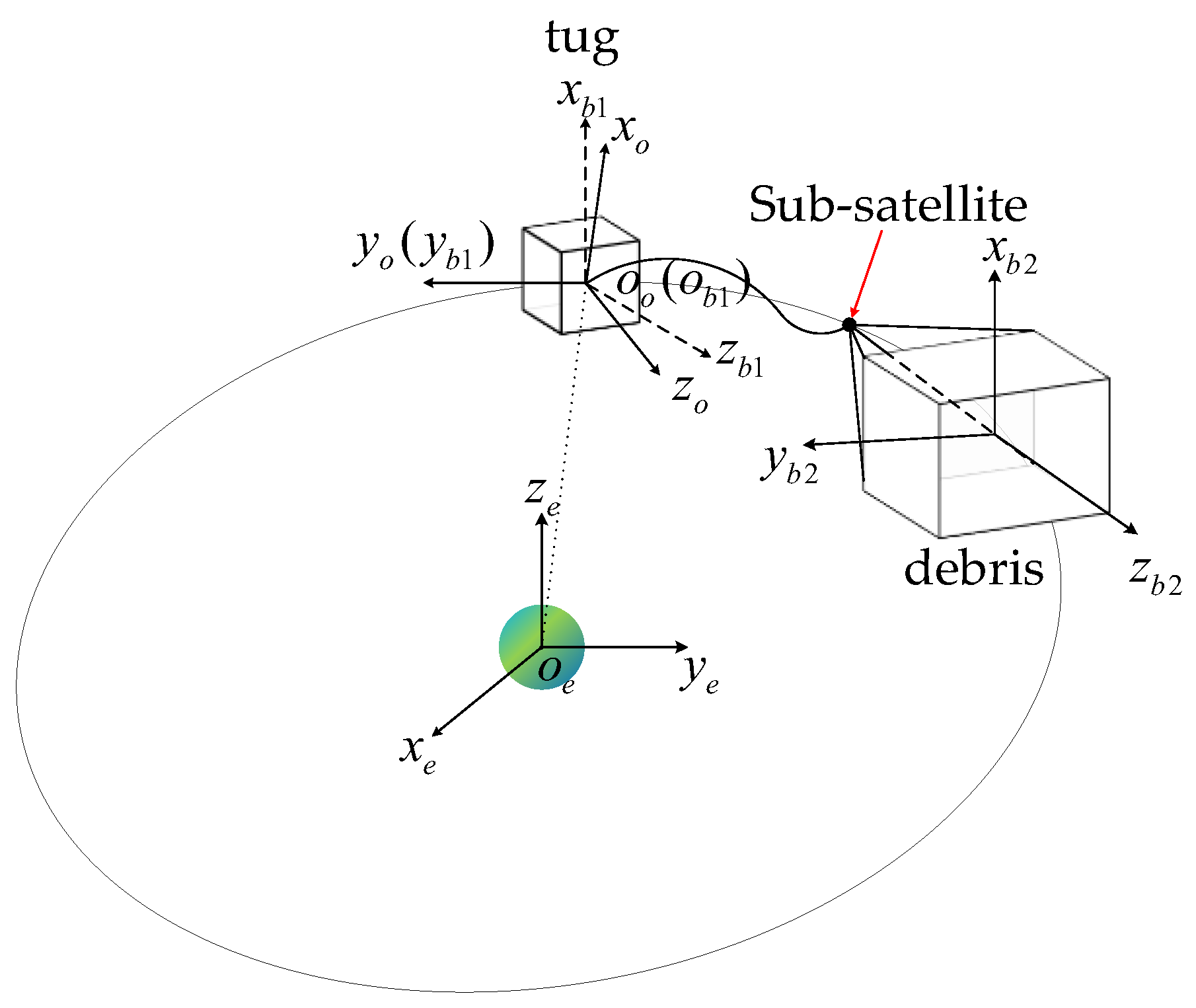
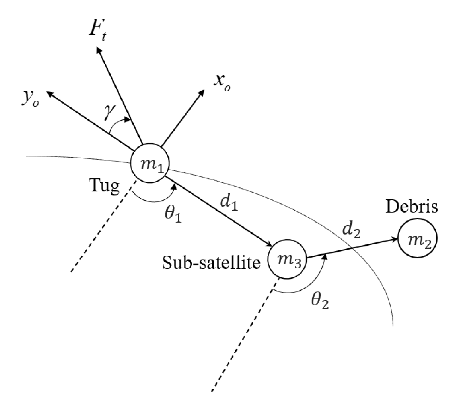
2. Problem Formulation

The two-segment tether towing system studied in this paper is shown in Figure 1. The system consists of a tug, a sub-satellite, a piece of space debris, and two segments of elastic tethers. The sub-satellite is released by the tug, and the second segment tethers are released by the sub-satellite to capture the space debris. Both the tug and the debris are regarded as rigid bodies. The sub-satellite, whose size is small compared to the length of the tether, can be regarded as a particle. The two parts of the tethers are regarded as massless spring-damper systems and can only be tensioned. The first part is released by the tug. The second part, which is attached to the ends of the debris, is released by the sub-satellite. To describe the kinematic relations of the components accurately, three right-handed frames are introduced. The orbit frame F o ( o o x o y o z o ) has its origin o o located at the mass center of the tug. The x o -axis points away from the Earth’s center to o o , the y o -axis is the flight direction of the tug, and the z o -axis conforms to the right-handed rule. The tug body frame F B 1 ( o b 1 x b 1 y b 1 z b 1 ) and the debris body frame F B 2 ( o b 2 x b 2 y b 2 z b 2 ) are placed at the mass centers of the tug and debris, respectively, whose axes are aligned with the principal moments of inertia axes of the two bodies.
The generalized coordinate vector of the system in the orbit frame is selected as
X = [ D 1 D 2 ϑ 1 ϑ 2 ]
where D 1 is the position vector which points from the mass center of the tug to the sub-satellite. D 2 is the position vector which points from the sub-satellite to the mass center of the debris. ϑ 1 and ϑ 2 are the attitude angles.
According to Kane’s method [28], the three-dimensional dynamic equation in the orbit frame can be derived as follows:
D ¨ 1 + 2 ω o × D ˙ 1 + ω o × D 1 × ω o + D 1 × ω ˙ o = F e x 3 / m 3 F e x 1 / m 1
D ¨ 2 + 2 ω o × D ˙ 2 + ω o × D 2 × ω o + D 2 × ω ˙ o = F e x 2 / m 2 F e x 3 / m 3
J 1 ω ˙ b 1 b + ω b 1 b × J 1 ω b 1 b = M e x 1
J 2 ω ˙ b 2 b + ω b 2 b × J 2 ω b 2 b = M e x 2
where m 1 is the mass of tug. m 2 is the mass of debris. m 3 is the mass of sub-satellite. ω b 1 b and ω b 2 b are the rotational angular velocities of the body frames with respect to the orbit frame. ω o is the orbital angular velocity. J 1 and J 2 are the inertia matrices of tug and debris, respectively. F e x 1 = F g 1 + F l 1 + F t F e x 2 = F g 2 + F l 2 F e x 3 = F g 3 F l 1 F l 2 M e x 1 = M g 1 + M l 1 + M c 1 M e x 2 = M g 2 + M l 2 + M c 2 . F l 1 is the tension of the first-part tether. F l 2 is the tension of the second part ones. F g i and M g i are the force and moment caused by the gravity gradient force. M c i is the control moment.
The tethers are considered as spring-damper systems [10]. The tether material is assumed to have a linear spring constant k i , a damping coefficient c i , and unstretched length l i 0 . The tether force is given as follows:
F l i = k i L i l i 0 l i + c i d l i l i 0 , L i > l i 0 , L i l i 0
where L i is the direction vector of each tether and l i is the unit vector along the tether.
The three-dimensional dynamics described by Equations (2)–(5) are too complicated, which is not suitable for the stability analysis. Hence, the following assumptions are made to simplify the system in the orbital plane: (1) Ignoring rigid body attitude, the tug, the sub-satellite, and the debris are all regarded as particles. (2) The system operates in an ideal Keplerian orbit. (3) The tethers in the second segment are simplified into an equivalent tether. Its physical coefficient is equal to the sum of all second-part tethers. (4) The out-of-plane orbit motion of the system is ignored.
Figure 2 shows the simplified system schematic diagram. d 1 is the distance between the tug and the sub-satellite. d 2 is the distance between the sub-satellite and the debris. θ 1 is the in-plane angle between the first-part tether and the negative direction of the x o -axis. θ 2 is the in-plane angle between the equivalent tether and the negative direction of the x o -axis. F t is the thrust of the tug. γ is the angle between the thrust and the y o -axis.
Based on Equation (1) and the assumptions, the generalized coordinate of the simplified system is X s = [ d 1 d 2 θ 1 θ 2 ] . The dimensionless transformation relation is introduced as follows:
F ¯ i = F i m 1 ω 0 2 d 10
(   ) = d (   ) d f = 1 ω 0 d (   ) d t
where the superscript “ (   ) ” indicates differentiation with respect to the true anomaly f . Employing the transformations yields the following dimensionless dynamic equations
d 1 = d 1 ( θ 1 + 1 ) 2 d 1 ( 1 3 cos 2 θ 1 ) μ 1 d 10 F ¯ l 1 + μ 3 d 10 F ¯ l 2 cos ( θ 2 θ 1 ) + F ¯ t d 10 sin ( θ 1 + γ )
d 2 = d 2 ( θ 2 + 1 ) 2 d 2 ( 1 3 cos 2 θ 2 ) μ 2 d 10 F ¯ l 2 + μ 3 d 10 F ¯ l 1 cos ( θ 2 θ 1 )
θ 1 = 3 2 sin 2 θ 1 2 d 1 d 1 ( θ 1 + 1 ) + μ 3 d 10 F ¯ l 2 d 1 sin ( θ 2 θ 1 ) + d 10 F ¯ t d 1 cos ( θ 1 + γ )
θ 2 = 3 2 sin 2 θ 2 μ 3 d 10 F ¯ l 1 d 2 sin ( θ 2 θ 1 ) 2 d 2 d 2 ( θ 2 + 1 )
where μ 1 , μ 2 , and μ 3 are dimensionless constants defined as follows:
μ 1 = ( m 1 + m 3 ) m 1 m 1 m 3 ,   μ 2 = ( m 2 + m 3 ) m 1 m 2 m 3 ,   μ 3 = m 1 m 3

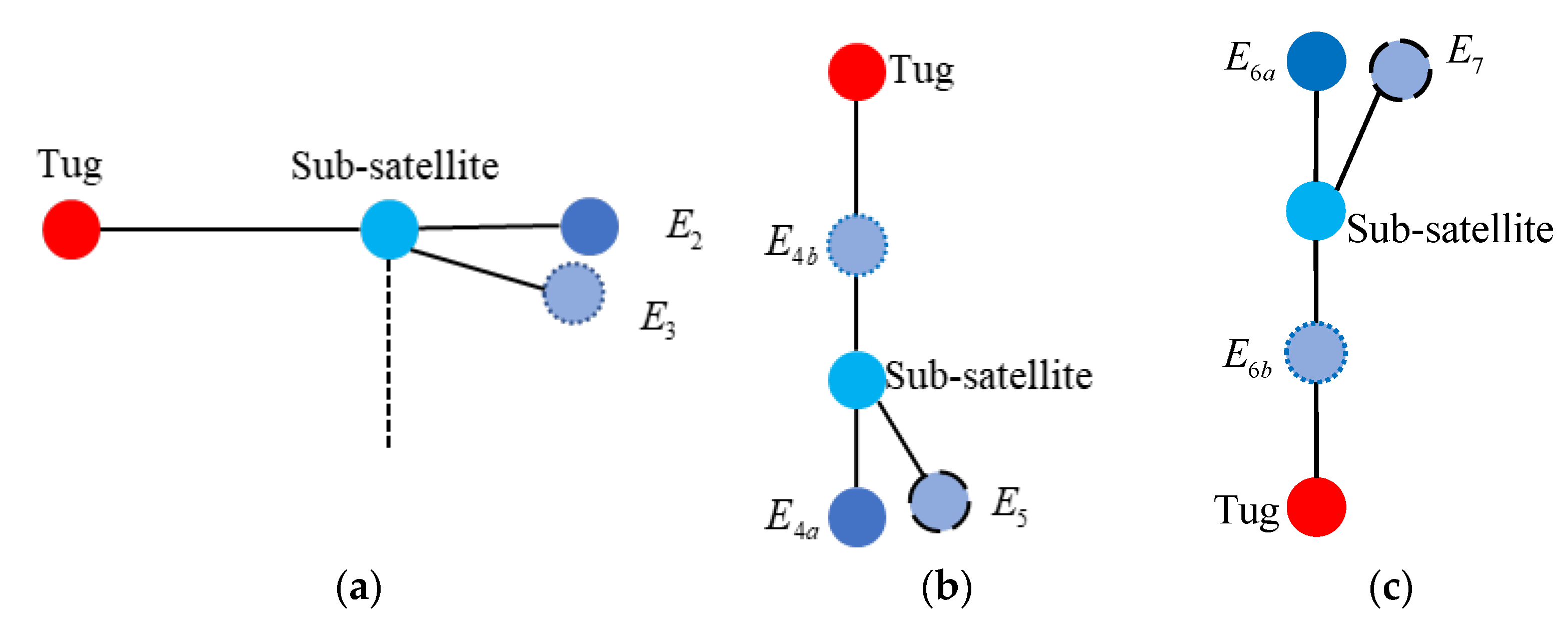
3. Equilibria and Stability Analysis

3.1. Equilibrium Configurations of the System

In order to ensure the stability of the towing process, it is necessary to figure out the equilibrium configurations of the system with constant thrust. To obtain the equilibrium configurations, the derivative terms of d 1 , d 2 , θ 1 , and θ 2 are set to zero in Equations (9)–(12). One obtains
3 d 1 cos 2 θ 1 μ 1 d 10 d ¯ l 1 + μ 3 d 10 F ¯ l 2 cos ( θ 2 θ 1 ) + F ¯ t d 10 sin ( θ 1 + γ ) = 0
3 d 2 cos 2 θ 2 μ 2 d 10 F ¯ l 2 + μ 3 d 10 F ¯ l 1 cos ( θ 2 θ 1 ) = 0
3 2 sin 2 θ 1 + μ 3 d 10 F ¯ l 2 d 1 sin ( θ 2 θ 1 ) + d 10 F ¯ t d 1 cos ( θ 1 + γ ) = 0
3 2 sin 2 θ 2 μ 3 d 10 F ¯ l 1 d 2 sin ( θ 2 θ 1 ) = 0
According to Equations (14) and (15), the relationship between F ¯ l i and F ¯ t can be given by
F ¯ l 1 = μ 2 ( 3 d 1 cos 2 θ 1 + F ¯ t d 10 sin ( θ 1 + γ ) ) + 3 μ 3 d 2 cos 2 θ 2 cos ( θ 2 θ 1 ) ( μ 1 μ 2 μ 3 2 cos 2 ( θ 2 θ 1 ) ) d 10
F ¯ l 2 = 3 d 2 μ 2 d 10 cos 2 θ 2 + μ 3 μ 2 F ¯ l 1 cos ( θ 2 θ 1 )
When γ = 0 , the direction of the thrust is along the y o -axis. The solution to Equations (16) and (17) is given as
E 1 : θ 1 e = π / 2 ,   θ 2 e = π / 2
In the equilibrium configuration E 1 , the three masses remain in a straight line along the y o -axis (local horizontal). Combined with Equation (6), θ 1 e = π / 2 and θ 2 e = π / 2 are substituted into Equations (14) and (15). The equilibrium solutions for tether length can be obtained as follows:
d 1 e = μ 2 F ¯ t ( μ 1 μ 2 μ 3 2 ) k 1 + d 10
d 2 e = μ 3 k 1 ( d 1 e d 10 ) μ 2 k 2 + d 20
As shown in Equations (21) and (22), d 1 e is affected by the thrust. The value of d 2 e is related to the first-part tether length.
Let γ 0 ; the solutions to Equations (16) and (17) are
E 2 : θ 1 e = π 2 ,   θ 2 e = π 2 ,   E 3 : θ 1 e = π 2 ,   θ 2 e = arcsin ( μ 2 μ 3 d 10 F ¯ t cos γ 3 ( μ 1 μ 2 μ 3 2 ) d 2 e ) E 4 : θ 1 e = 0 ,   θ 2 e = 0 / π ,   E 5 : θ 1 e = 0 ,   θ 2 e = arccos ( 3 μ 3 d 1 μ 3 d 10 F ¯ t sin γ 3 μ 1 d 2 e ) E 6 : θ 1 e = π ,   θ 2 e = 0 / π ,   E 7 : θ 1 e = π ,   θ 2 e = arccos ( μ 3 d 1 μ 3 d 10 F ¯ t sin γ 3 μ 1 d 2 e )
In the configuration E 2 , the three masses remain in the same state as the configuration E 1 . In the configurations E 4 and E 6 , the three masses line up on the x o -axis (local vertical). The equilibrium solution θ 2 e in the configurations E 3 , E 5 , and E 7 is determined by γ , d 1 e , and d 2 e and can be solved in the same way as in E 1 .
Figure 3 gives the schematic diagrams of the solutions shown in Equation (23). The red ball represents the tug, the light blue ball represents the sub-satellite, and the other balls correspond to the debris in each configuration.

3.2. Stability of Equilibrium Configuration

Define x = [ x 1 , x 2 , x 3 , x 4 ] T , where x 1 = θ 1 θ 1 e , x 2 = θ 1 , x 3 = θ 2 θ 2 e and x 4 = θ 2 . The new coordinates x represent the variations of θ 1 and θ 2 from their equilibrium solutions. The new equilibrium solutions are x e = [ 0 , 0 , 0 , 0 ] T . Then Equations (16) and (17) can be linearized about x 1 e and x 2 e as follows:
x ˙ 1 = x 2 x ˙ 2 = C 1 x 1 + C 2 x 3 x ˙ 3 = x 4 x ˙ 4 = C 3 x 1 + C 4 x 3
where C i are constants defined as follows:
C 1 = 3 cos 2 θ 1 e μ 3 d 10 d 1 e F ¯ l 2 cos ( θ 2 e θ 1 e ) F ¯ t d 10 d 1 e sin ( θ 1 e + γ ) , C 2 = μ 3 d 10 d 1 e F ¯ l 2 cos ( θ 2 e θ 1 e ) , C 3 = μ 3 d 10 d 2 e F ¯ l 1 cos ( θ 2 e θ 1 e ) , C 4 = 3 cos 2 θ 2 e μ 3 d 10 d 2 e F ¯ l 1 cos ( θ 2 e θ 1 e )
Equation (24) is rewritten in matrix form as follows:
x ˙ = C x = 0 1 0 0 C 1 0 C 2 0 0 0 0 1 C 3 0 C 4 0 x 1 x 2 x 3 x 4
The characteristic equation can be obtained as
a 0 λ 4 + a 1 λ 3 + a 2 λ 2 + a 3 λ + a 4 = 0
where a 0 = 1 , a 1 = 0 , a 2 = ( C 1 + C 4 ) , a 3 = 0 , and a 4 = C 1 C 4 C 2 C 3 . It can be found that a 1 and a 3 are zeros for equilibrium configuration. This implies that there is no asymptotic stable equilibrium. There can be marginal stability with imaginary values for all λ i , provided that a 0 > 0 , a 2 > 0 , a 4 > 0 , and a 2 2 > 4 a 0 a 4 .
By solving Equation (22), the eigenvalues can be obtained:
λ 1 , 2 = ± C 1 2 + C 4 2 ( C 1 C 4 ) 2 + 4 C 2 C 3 2 λ 3 , 4 = ± C 1 2 + C 4 2 + ( C 1 C 4 ) 2 + 4 C 2 C 3 2
The system physical parameters are set as follows:
m 1 = 500   kg ,   m 2 = 2000   kg ,   m 3 = 8   kg ,   F t = 150   N d 10 = 100   m ,   d 20 = 8.5   m ,   k i = 264   N / m ,   c i = 8   Ns / m
The orbit altitude of the system is 700 km. In E 1 , it can be shown that a 0 = 1 , a 2 > 0 , and a 4 > 0 . It can also be shown that a 2 2 > 4 a 0 a 4 . One can determine λ i as follows:
λ 1 = 35.1074 i ,   λ 2 = 35.1074 i ,   λ 3 = 2.7534 × 10 14 + 5.1636 × 10 2 i ,   λ 4 = 2.7534 × 10 14 5.1636 × 10 2 i
As can be seen from Equation (30), λ i and λ i are on the imaginary axis, but they are not multiple roots. There are no roots of the Jodan form; the equilibrium point is stable according to Theorem 4.5 [49].
Considering γ = 1 , it can be shown that a 0 = 1 , a 2 > 0 , a 4 > 0 , and a 2 2 > 4 a 0 a 4 in the line configurations E 2 and E 4 a ( θ 1 e = 0 , θ 2 e = 0 ) . Similar to E 1 , they are also the stability conditions. Taking E 4 a ( θ 1 e = 0 , θ 2 e = 0 ) as an example, one can determine the λ i as follows:
λ 1 = 32.2957 i ,   λ 2 = 32.2957 i ,   λ 3 = 2.1316 × 10 14 + 4.5799 × 10 2 i ,   λ 4 = 2.1316 × 10 14 4.5799 × 10 2 i
However, the configurations E 4 b ( θ 1 e = 0 , θ 2 e = π ) and E 6 do not satisfy the stability condition because the corresponding eigenvalues have real roots. Hence, these equilibriums are unstable.
In configurations E 3 , E 5 , and E 7 , it can be shown that a 0 = 1 , a 2 > 0 , and a 4 > 0 . It can also be shown that a 2 2 > 4 a 0 a 4 . Hence, the equilibrium is stable. One can determine the λ i as follows:
λ 1 = 47.6853 i ,   λ 2 = 47.6853 i ,   λ 3 = 1.5632 × 10 13 + 1.2312 × 10 3 i ,   λ 4 = 1.5632 × 10 13 1.2312 × 10 3 i
Taking E 1 as an example, it can be obtained that F l 1 e = 120.096   N , F l 2 e = 119.617   N , d 1 e = 100.487   m , and d 2 e = 8.9869   m when the system is stable by substituting the parameters in Equation (29) into Equations (18), (19), (21) and (22). The analysis results are verified by simulation in Section 5.1.

4. Libration Controller Design

In this section, based on the sliding mode control scheme, a controller of in-plane libration angles is designed. The equilibrium solution solved in Section 3 is taken as the desired state. In towing mission, the angles will lead to serious tether librations, which will cause the system configuration to change continuously. To overcome the change, more fuel is required to complete a predetermined mission than the desired state. So, it is desirable for the in-plane libration angles to be maintained at the state to save fuel and ensure mission safety. It is assumed that the tug and the sub-satellite are equipped with air jets that can be used to adjust their positions. The in-plane libration angles can be suppressed to the desired state and maintained at equilibrium by applying external torques. Adding the control inputs into Equations (11) and (12) yields
θ 1 = 3 2 sin 2 θ 1 2 d 1 d 1 ( θ 1 + 1 ) + m 1 d 10 F ¯ l 2 m 3 d 1 sin ( θ 2 θ 1 ) + d 10 F ¯ t d 1 cos θ 1 + u 1
θ 2 = 3 2 sin 2 θ 2 m 1 d 10 F ¯ l 1 m 3 d 2 sin ( θ 2 θ 1 ) 2 d 2 d 2 ( θ 2 + 1 ) + u 2
Equations (33) and (34) are rewritten in general form as follows:
θ 1 = f 1 ( θ 1 , θ 2 ) + u 1 + d d i s 1
θ 2 = f 2 ( θ 1 , θ 2 ) + u 2 + d d i s 2
where
f 1 ( θ 1 , θ 2 ) = 3 2 sin 2 θ 1 + m 1 F ¯ l 2 m 3 sin ( θ 2 θ 1 ) + F ¯ t cos θ 1
f 2 ( θ 1 , θ 2 ) = 3 2 sin 2 θ 2 m 1 d 1 F ¯ l 1 m 3 d 2 sin ( θ 2 θ 1 )
d d i s 1 = 2 d 1 d 1 ( θ 1 + 1 )
d d i s 2 = 2 d 2 d 2 ( θ 2 + 1 )
where d d i s 1 and d d i s 2 are time-varying, related to the values of d 1 , d 2 , d 1 , d 2 , θ 1 , and θ 2 . Assume d d i s 1 D 1 and d d i s 2 D 2 , in which D 1 and D 2 are positive constants.
Define ε θ 1 = θ 1 θ 1 d and ε θ 2 = θ 2 θ 2 d . Design sliding surfaces as follows:
s 1 = ε ˙ θ 1 + c s 1 ε θ 1
s 2 = ε ˙ θ 2 + c s 2 ε θ 2
By taking the first derivative of Equations (41) and (42), we obtain
s ˙ 1 = ε ¨ θ 1 + c s 1 ε ˙ θ 1 = θ 1 + c s 1 θ 1
s ˙ 2 = ε ¨ θ 2 + c s 2 ε ˙ θ 2 = θ 2 + c s 2 θ 2
The exponential reaching law is adopted to drive the system to the sliding mode surface
s ˙ = k s ε sgn s
where k > 0 and ε > 0 . By combining Equation (45) with Equations (43) and (44), the in-plane libration angle control forces can be designed as
u 1 = k s 1 s 1 ε s 1 sgn s 1 c s 1 θ 1 f 1
u 2 = k s 2 s 2 ε s 2 sgn s 2 c s 2 θ 2 f 2
with
ε ˙ s i = σ i s i
where σ i is a positive constant.
Define s = [ s 1 , s 2 ] T . Choose the following Lyapunov function candidate
V = 1 2 s T s + 1 2 σ s 1 ( ε s 1 D 1 ) 2 + 1 2 σ s 2 ( ε s 2 D 2 ) 2
whose time derivative is
V ˙ = s T s ˙ + ε ˙ s 1 σ s 1 ( ε s 1 D 1 ) + ε ˙ s 2 σ s 2 ( ε s 2 D 2 )
Due to ε ˙ s i = σ i s i , we obtain
V ˙ = s 1 s ˙ 1 + s 2 s ˙ 2 + ( ε s 1 D 1 ) s 1 + ( ε s 2 D 2 ) s 2
Combined with Equations (35), (36), (43) and (44), Equation (51) can be reformulated as
V ˙ = s 1 ( f 1 + u 1 + d d i s 1 + c s 1 θ 1 ) + s 2 ( f 2 + u 2 + d d i s 2 + c s 2 θ 2 ) + ( ε s 1 D 1 ) s 1 + ( ε s 2 D 2 ) s 2 = s 1 ( k s 1 s 1 ε s 1 sgn s 1 ) + s 2 ( k s 2 s 2 ε s 2 sgn s 2 ) + s 1 d d i s 1 + s 2 d d i s 2 + ( ε s 1 D 1 ) s 1 + ( ε s 2 D 2 ) s 2 = k s 1 s 1 2 k s 2 s 2 2 + s 1 d d i s 1 + s 2 d d i s 2 D 1 s 1 D 2 s 2
In terms of d d i s 1 D 1 and d d i s 2 D 2 , we obtain
s 1 d d i s 1 D 1 s 1 0 s 2 d d i s 2 D 2 s 2 0
Thus,
V ˙ k s 1 s 1 2 k s 2 s 2 2
When s [0, 0]T, it is clear that V ˙ is negative. Hence, the system will converge to the sliding surface and reach the equilibrium asymptotically along the sliding surface. Therefore, the in-plane libration angles could converge to the desired state with u 1 and u 2 .

5. Simulation Results

To verify the results of theoretical analysis and the effectiveness of the designed controller, simulations are carried out with initial physical parameters shown in Equation (29). The simulation results of the equilibrium configuration E 1 are shown in Section 5.1. Those of the system with control are shown in Section 5.2.

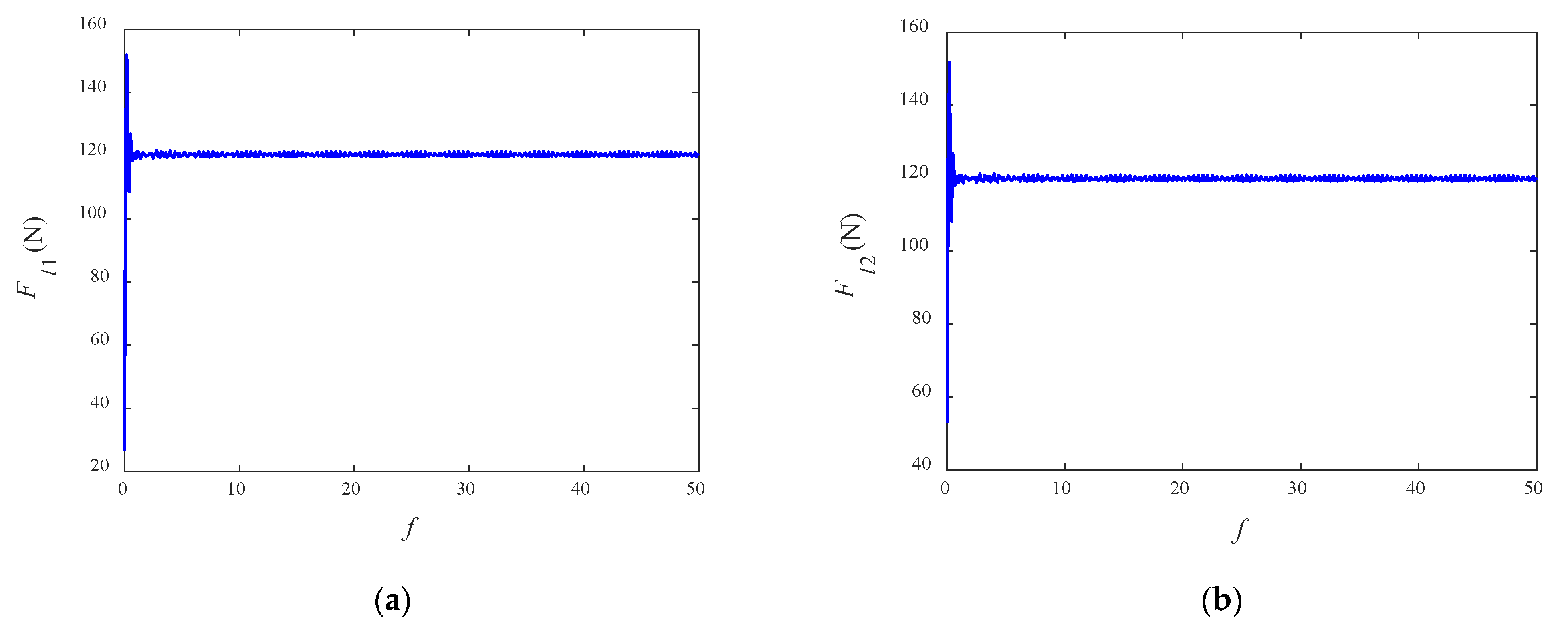
5.1. Simulations for Equilibrium Configuration

In the following simulation, it is assumed that the initial state deviates from the equilibrium state and the tethers are tensioned. The physical parameters shown in Equation (29) and the initial values [ d 1 , d 1 , θ 1 , θ 1 , d 2 , d 2 , θ 2 , θ 2 ] = [ 100.1 , 0 , 1.5 , 0 , 8.7 , 0 , 1.4 , 0 ] are used for the numerical simulation of Equations (9)–(12). The results are shown as follows:
Figure 4 shows the variations of the generalized coordinate X s . It can be found that d 1 and d 2 show large libration amplitudes, which are driven by d d i s 1 and d d i s 2 , and their maximum values are 100.621 and 9.121. Since the initial condition deviates from the configuration E 1 and the tether is tensioned, the tether length will change at the beginning, so that d 1 and d 2 are non-zero and d d i s 1 and d d i s 2 occur. When the system reaches the equilibrium state at f = 0.8 , the tether length and the other coordinates tend to be stable. The equilibrium positions of d 1 and d 2 are equal to 100.487 and 8.9869, respectively, while those of θ 1 and θ 2 are equal to π / 2 , which is in good agreement with the analysis results.
It can be seen from Figure 5 that when the system moves towards the equilibrium state, the variations of tensions in the two segments of tethers show similar tendencies to d 1 and d 2 at the initial moment. When the equilibrium is reached, the tether tensions are also close to the value of F l 1 e and F l 2 e . They vary periodically with respect to f . As a result, the simulation results for equilibrium configuration support those of theoretical analysis as exhibited in Section 3.2.

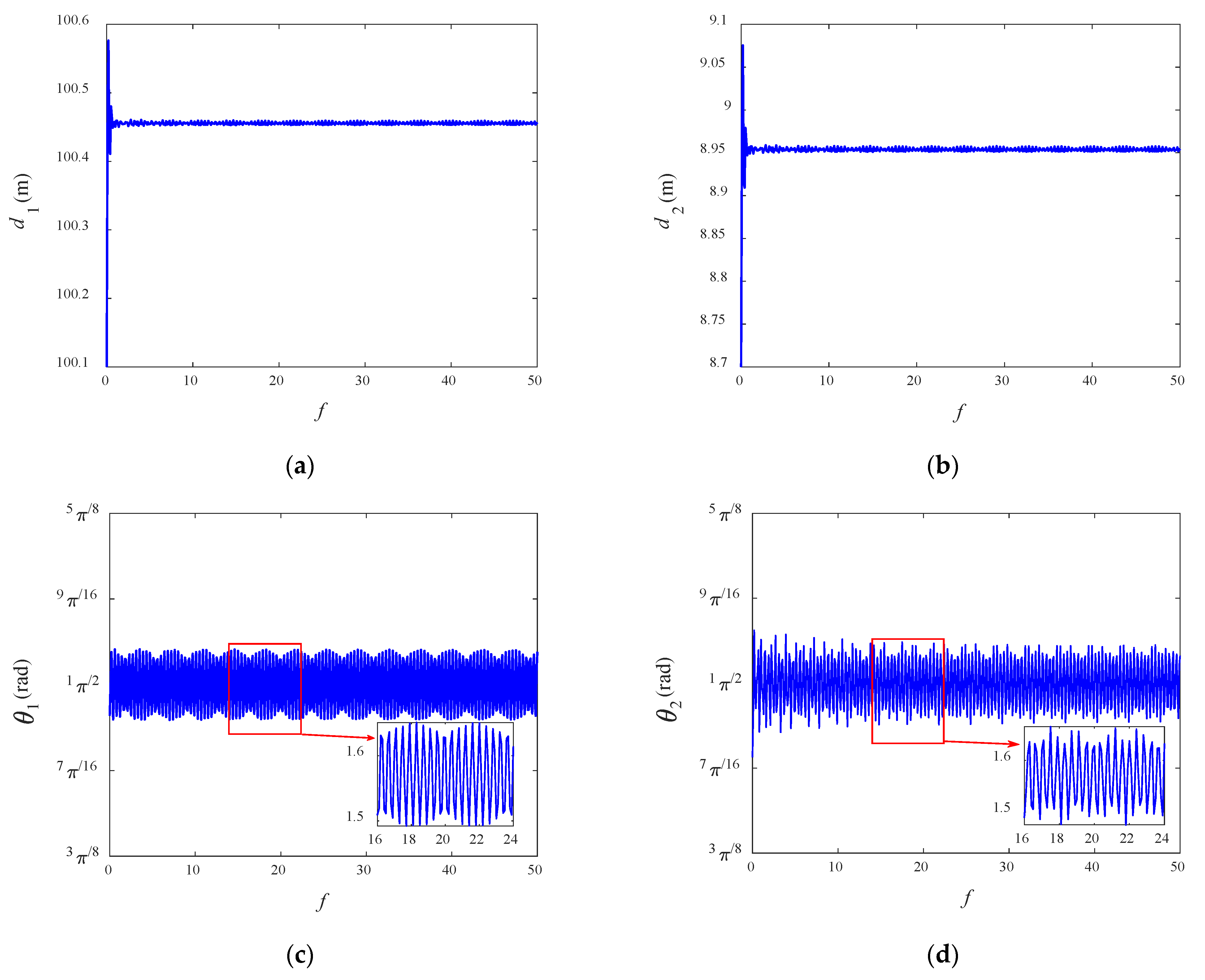
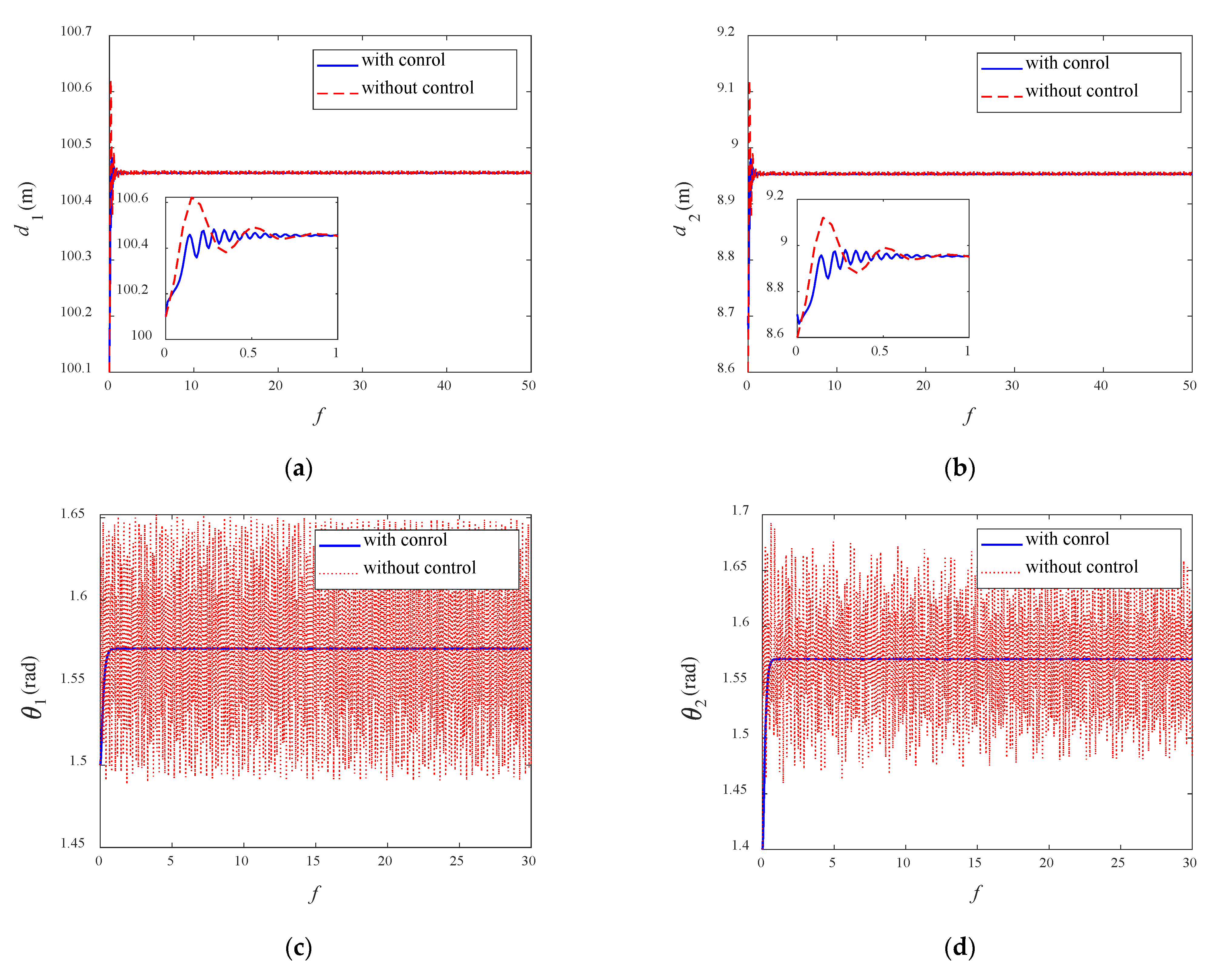
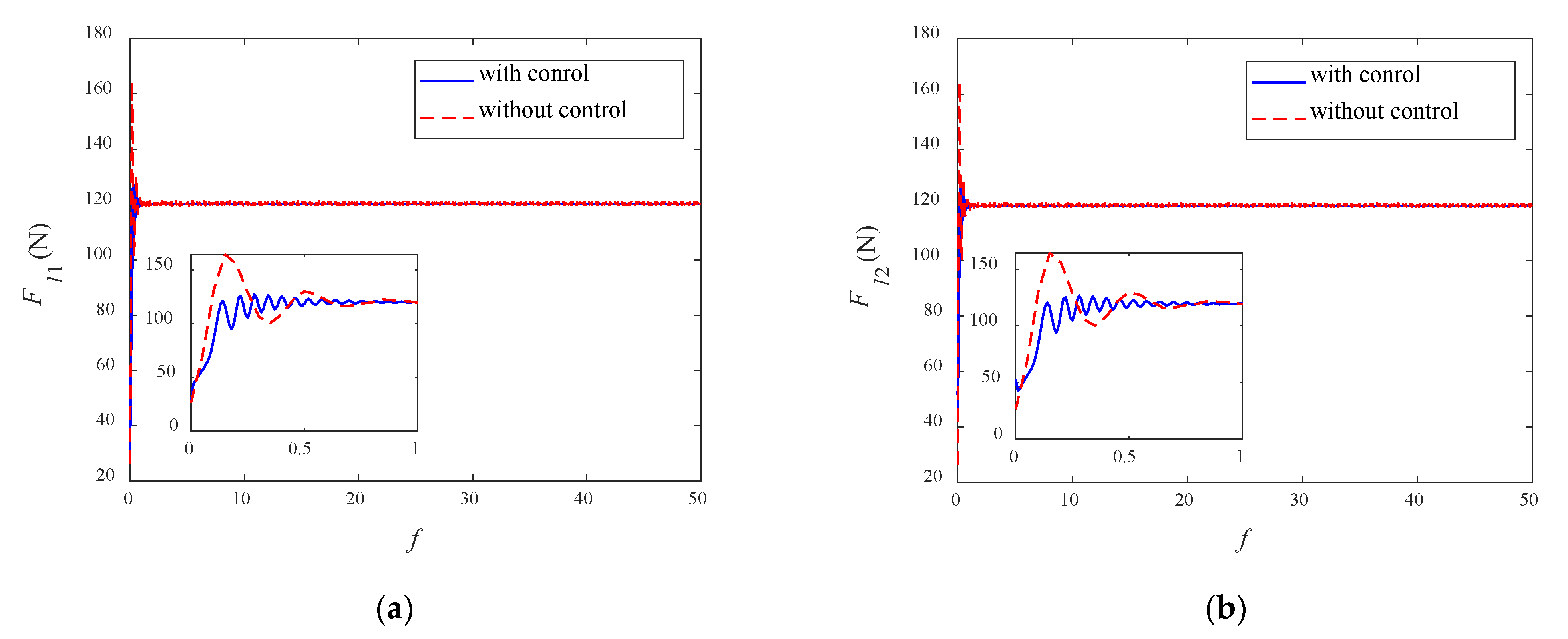
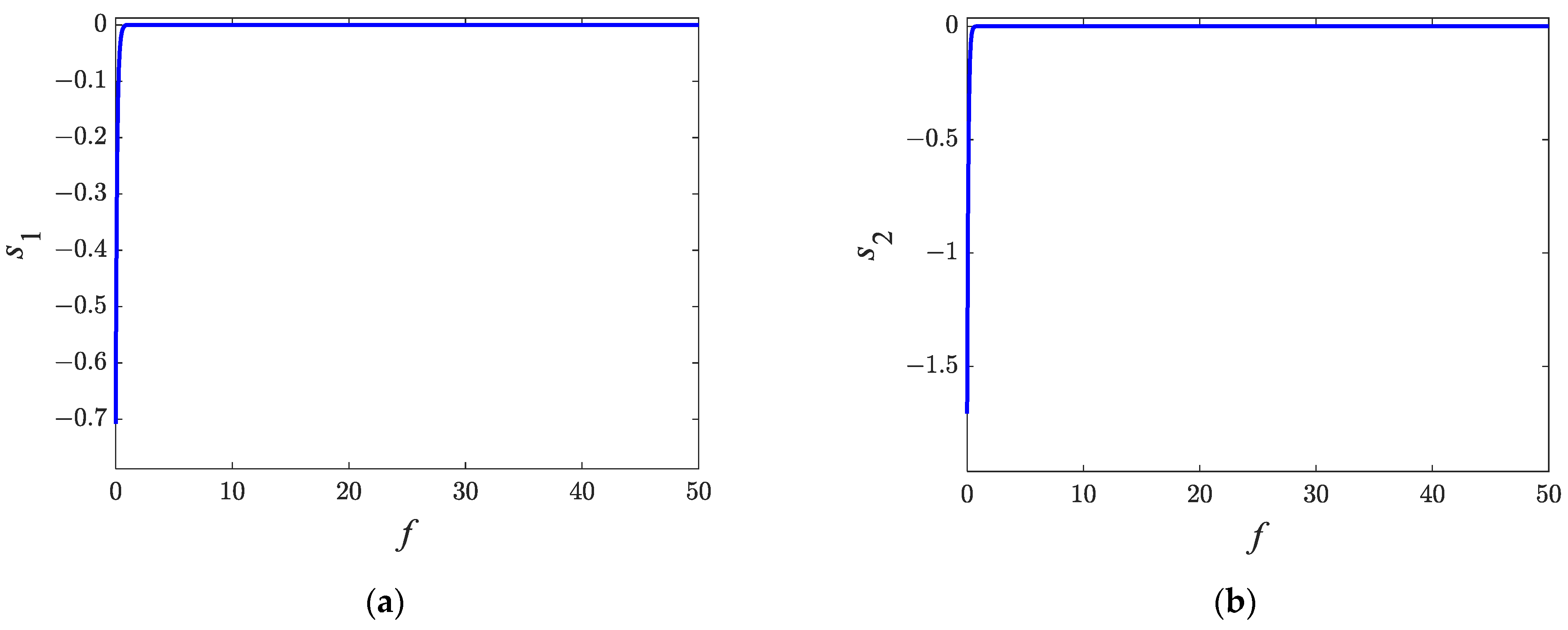
5.2. Simulations for Libration Controller

As can be seen from the simulation results in Section 5.1, the changes of each generalized coordinate at the initial moment are obvious. The large libration amplitudes may result in additional fuel consumption and configuration failure. So, it is necessary to control the variations. To verify the effect of the libration controller, the controller parameters as selected as follows:
c s 1 = 10 ,   ε s 1 = 0.01 ,   k s 1 = 10 c s 2 = 10 ,   ε s 2 = 0.01 ,   k s 2 = 10
Figure 6 shows the variations of generalized coordinates with the action of the designed controller. It can be seen from the figures that the system reaches the desired state at f = 0.8 . The librations of the in-plane angles are effectively suppressed. Compared with the results in Figure 4, the in-plane angles are well maintained at π / 2 to achieve the purpose of fuel saving. At the same time, the librations along the tether length at the initial moment are alleviated. It can be seen from Equations (9)–(12) that the in-plane angles and librations along the tether length are coupled with each other. When the former is suppressed, it is easy to stabilize the variations of the tether length.
Figure 7 shows the variations of the tethers’ tension under the action of controller compared with the result of Figure 5. The variation trends are almost the same as those of d 1 and d 2 . This is due to the fact that when the system is in equilibrium, F l 1 and F l 2 are approximately the linear function of d 1 and d 2 whose slope is the stiffness coefficient of the tether.
The control results corresponding to those in Figure 6 and Figure 7 are listed in Table 1. It can be seen from the table that the maximum values of the controlled variables after control are all smaller than those before control. This shows that the librations of the controlled variables are suppressed and the effectiveness of the libration controller is confirmed. In addition, it takes almost the same time for all the variables to approach the equilibrium state before and after control. On the other hand, adjusting the controller parameters can allow the system to reach the desired state faster.
Figure 8 shows the variations of the sliding mode surfaces. Figure 9 shows the variations of the control forces u 1 and u 2 . When s 1 and s 2 approach zero, θ 1 and θ 2 reach the desired state and the air jets stop working. It can be seen from Figure 9 that u 1 is positive and changes along the x o -axis of the orbit frame while u 2 varies in the negative direction of the x o -axis. To satisfy this control requirement and guarantee the desired performance, the tug and the sub-satellite are required to provide two opposing control torques to force the in-plane libration angles to the desired state.
Table 2 gives the statistical statements of Monte Carlo results about maximum control values and settling times. The random initial value range of each variable is set as d 1 [ 99.8 , 100.2 ] , d 2 [ 8.2 , 8.8 ] , θ 1 [ 1.4 , 1.7 ] , and θ 2 [ 1.4 , 1.7 ] . All the cases can converge within f = 1.05 .

6. Conclusions

This paper develops a two-segment tethered towing system. A dynamic model is derived in the orbit frame. A set of equilibrium solutions are obtained based on the in-plane simplified model by considering the flexibility of the tethers. An in-plane libration controller is proposed by using the sliding mode control approach, where the equilibrium solution is taken as a desired state. Simulations with control and without control are performed to evaluate the performance of the controller. The following conclusions are drawn:
(1)
Seven sets of equilibrium configurations are given. The configuration in which the tug, sub-satellite, and debris remain in a straight line along the local horizontal is stable.
(2)
An in-plane libration controller is designed. According to the Lyapunov function, the system will converge to the sliding surface asymptotically. The system will reach the equilibrium asymptotically with the action of the designed libration controller. It can be seen from the Monte Carlo results that the control can converge within a short time.
(3)
It can be found from the simulation results that the librations in the direction of tether length can be effectively suppressed with the suppression of the oscillations of the in-plane angles. This is attributed to the coupling characteristics between in-plane angles and the tether length. As a result, the system under the action of the designed controller can reach the desired state while the librations of in-plane angles are effectively suppressed.

Author Contributions

Conceptualization, T.C. and J.K.; writing—original draft preparation, S.C.; writing—review and editing, S.C., W.C., T.C. and J.K.; visualization, S.C.; supervision, W.C. All authors have read and agreed to the published version of the manuscript.

Funding

This work was supported by the National Natural Science Foundation of China (Grant Nos. 12102174 and 12232011) and the Research Fund of State Key Laboratory of Mechanics and Control of Mechanical Structures (Nanjing University of Aeronautics and Astronautics) (Grant No. MCMS-I-0122K01).

Data Availability Statement

Not applicable.

Conflicts of Interest

The authors declare no conflict of interest.

References

  1. Muelhaupt, T.J.; Sorge, M.E.; Morin, J.; Wilson, R.S. Space traffic management in the new space era. J. Space Saf. Eng. 2019, 6, 80–87. [Google Scholar] [CrossRef]
  2. Shan, M.; Guo, J.; Gill, E. Deployment dynamics of tethered-net for space debris removal. Acta Astronaut. 2017, 132, 293–302. [Google Scholar] [CrossRef]
  3. Botta, E.M.; Sharf, I.; Misra, A.K. Contact dynamics modeling and simulation of tether nets for space-debris capture. J. Guid. Control Dyn. 2017, 40, 110–123. [Google Scholar] [CrossRef]
  4. Botta, E.M.; Sharf, I.; Misra, A.K.; Teichmann, M. On the simulation of tether-nets for space debris capture with vortex dynamics. Acta Astronaut. 2016, 123, 91–102. [Google Scholar] [CrossRef]
  5. Benvenuto, R.; Lavagna, M.; Salvi, S. Multibody dynamics driving GNC and system design in tethered nets for active debris removal. Adv. Space Res. 2016, 58, 45–63. [Google Scholar] [CrossRef]
  6. Sharf, I.; Thomsen, B.; Botta, E.M.; Misra, A.K. Experiments and simulation of a net closing mechanism for tether-net capture of space debris. Acta Astronaut. 2017, 139, 332–343. [Google Scholar] [CrossRef]
  7. Yue, S.; Li, M.; Zhao, Z.; Du, Z.; Wu, C.; Zhang, Q. Parameter Analysis and Experiment Validation of Deployment Characteristics of a Rectangular Tether-Net. Aerospace 2023, 10, 115. [Google Scholar] [CrossRef]
  8. Lv, S.; Zhang, H.; Zhang, Y.; Ning, B.; Qi, R. Design of an integrated platform for active debris removal. Aerospace 2022, 9, 339. [Google Scholar] [CrossRef]
  9. Mark, C.P.; Kamath, S. Review of active space debris removal methods. Space Policy 2019, 47, 194–206. [Google Scholar] [CrossRef]
  10. Stadnyk, K.; Ulrich, S. Validating the Deployment of a Novel Tether Design for Net-Based Orbital Debris Removal Missions. In Proceedings of the AIAA SciTech Forum and Exposition, Orlando, FL, USA, 6–10 January 2020; pp. 592–611. [Google Scholar]
  11. Jung, W.; Mazzoleni, A.P.; Chung, J. Dynamic analysis of a tethered satellite system with a moving mass. Nonlinear Dyn. 2014, 75, 267–281. [Google Scholar] [CrossRef]
  12. Abouelmagd, E.I.; Guirao, J.L.G.; Hobiny, A.; Alzahrani, F. Dynamics of a tethered satellite with variable mass. Discret. Contin. Dyn. Syst. Ser. S 2015, 8, 1035–1045. [Google Scholar] [CrossRef]
  13. Abouelmagd, E.I.; Guirao, J.L.G.; Vera, J.A. Dynamics of a dumbbell satellite under the zonal harmonic effect of an oblate body. Commun. Nonlinear Sci. 2015, 20, 1057–1069. [Google Scholar] [CrossRef] [Green Version]
  14. Pang, Z.; Jin, D.; Yu, B.; Wen, H. Nonlinear normal modes of a tethered satellite system of two degrees of freedom under internal resonances. Nonlinear Dyn. 2016, 85, 1779–1789. [Google Scholar] [CrossRef]
  15. Aslanov, V.S.; Ledkov, A.S. Dynamics of towed large space debris taking into account atmospheric disturbance. Acta Astronaut. 2014, 225, 2685–2697. [Google Scholar] [CrossRef]
  16. Aslanov, V.S.; Yudintsev, V.V. Dynamics, analytical solutions and choice of parameters for towed space debris with flexible appendages. Adv. Space Res. 2015, 55, 660–667. [Google Scholar] [CrossRef]
  17. Aslanov, V.S.; Yudintsev, V.V. The motion of tethered tug–debris system with fuel residuals. Adv. Space Res. 2015, 56, 1493–1501. [Google Scholar] [CrossRef]
  18. Aslanov, V.S.; Misra, A.K.; Yudintsev, V.V. Chaotic attitude motion of a low-thrust tug-debris tethered system in a keplerian orbit. Acta Astronaut. 2017, 139, 419–427. [Google Scholar] [CrossRef]
  19. Aslanov, V.S.; Yudintsev, V.V. Chaos in tethered tug–debris system induced by attitude oscillations of debris. J. Guid. Control Dyn. 2019, 42, 1630–1637. [Google Scholar] [CrossRef]
  20. Aslanov, V.S. Stability of a pendulum with a moving mass: The averaging method. J. Sound Vib. 2019, 445, 261–269. [Google Scholar] [CrossRef]
  21. Lim, J.; Chung, J. Dynamic analysis of a tethered satellite system for space debris capture. Nonlinear Dyn. 2018, 94, 2391–2408. [Google Scholar] [CrossRef]
  22. Shan, M.; Shi, L. Comparison of tethered post-capture system models for space debris removal. Aerospace 2022, 9, 33. [Google Scholar] [CrossRef]
  23. Qi, R.; Misra, A.K.; Zuo, Z. Active debris removal using double-tethered space-tug system. J. Guid. Control Dyn. 2017, 40, 722–730. [Google Scholar] [CrossRef]
  24. Hovell, K.; Ulrich, S. Attitude stabilization of an unknown and spinning target spacecraft using a visco-elastic tether. In Proceedings of the 13th Symposium on Advanced Space Technologies in Robotics and Automation, Noordwijk, The Netherlands, 11–13 May 2015; pp. 1–8. [Google Scholar]
  25. Hovell, K.; Ulrich, S. Attitude stabilization of an uncooperative spacecraft in an orbital environment using visco-elastic tethers. In Proceedings of the AIAA Guidance, Navigation, and Control Conference, San Diego, CA, USA, 4–8 January 2016; pp. 1343–1358. [Google Scholar]
  26. Hovell, K.; Ulrich, S. Experimental validation for tethered capture of spinning space debris. In Proceedings of the AIAA Guidance, Navigation, and Control Conference, Grapevine, TX, USA, 9–13 January 2017; pp. 626–644. [Google Scholar]
  27. Hovell, K.; Ulrich, S. Postcapture dynamics and experimental validation of subtethered space debris. J. Guid. Control Dyn. 2018, 41, 519–525. [Google Scholar] [CrossRef]
  28. Yang, K.Y.; Misra, A.K.; Zhang, J.; Qi, R.; Lu, S.; Liu, Y. Dynamics of a debris towing system with hierarchical tether architecture. Acta Astronaut. 2020, 177, 891–905. [Google Scholar] [CrossRef]
  29. Abouelmagd, E.I.; Guirao, J.L.G.; Hobiny, A.; Alzahrani, F. Stability of equilibria points for a dumbbell satellite when the central body is oblate spheroid. Discret. Contin. Dyn. Syst. S 2015, 8, 1047–1054. [Google Scholar] [CrossRef]
  30. Hu, W.; Song, M.; Deng, Z. Energy dissipation/transfer and stable attitude of spatial on-orbit tethered system. J. Sound Vib. 2018, 412, 58–73. [Google Scholar] [CrossRef]
  31. Lian, X.; Liu, J.; Zhang, J.; Wang, C. Chaotic motion and control of a tethered-sailcraft system orbiting an asteroid. Commun. Nonlinear Sci. Numer. Simul. 2019, 77, 203–224. [Google Scholar] [CrossRef]
  32. Liu, J.F.; Qu, W.L.; Yuan, L.H.; Cui, N.G. Nonlinear dynamics of a space tethered system in the elliptic earth-moon restricted three-body system. J. Aerosp. Eng. 2019, 32, 04018139. [Google Scholar] [CrossRef]
  33. Sun, L.; Zhao, G.; Huang, H. Effect of mass variation on dynamics of tethered system in orbital maneuvering. Acta Astronaut. 2018, 146, 15–23. [Google Scholar] [CrossRef]
  34. Jin, D.P.; Hu, H.Y. Optimal control of a tethered subsatellite of three degrees of freedom. Nonlinear Dyn. 2006, 46, 161–178. [Google Scholar] [CrossRef]
  35. Sun, X.; Zhong, R. Switched propulsion force libration control for the low-thrust space tug system. Aerosp. Sci. Technol. 2018, 80, 281–287. [Google Scholar] [CrossRef]
  36. Wen, H.; Zhu, Z.H.; Jin, D.; Hu, H. Constrained tension control of a tethered space-tug system with only length measurement. Acta Astronaut. 2016, 119, 110–117. [Google Scholar] [CrossRef]
  37. Zhang, Z.; Yu, Z.; Zhang, Q.; Zeng, M.; Li, S. Dynamics and control of a tethered space-tug system using Takagi-Sugeno fuzzy methods. Aerosp. Sci. Technol. 2019, 87, 289–299. [Google Scholar] [CrossRef]
  38. Zhang, J.; Yang, K.; Qi, R. Dynamics and offset control of tethered space-tug system. Acta Astronaut. 2018, 142, 232–252. [Google Scholar] [CrossRef]
  39. Kang, J.; Zhu, Z.H.; Santaguida, L.F. Analytical and experimental investigation of stabilizing rotating uncooperative target by tethered space tug. IEEE Trans. Aerosp. Electron. Syst. 2021, 57, 2426–2437. [Google Scholar] [CrossRef]
  40. Razzaghi, P.; Al Khatib, E.; Bakhtiari, S. Sliding mode and SDRE control laws on a tethered satellite system to de-orbit space debris. Adv. Space Res. 2019, 64, 18–27. [Google Scholar] [CrossRef]
  41. Chu, Z.; Di, J.; Cui, J. Hybrid tension control method for tethered satellite systems during large tumbling space debris removal. Acta Astronaut. 2018, 152, 611–623. [Google Scholar] [CrossRef]
  42. Xu, S.; Sun, G.; Ma, Z.; Li, X. Fractional-order fuzzy sliding mode control for the deployment of tethered satellite system under input saturation. IEEE Trans. Aerosp. Electron. Syst. 2018, 55, 747–756. [Google Scholar] [CrossRef]
  43. Xu, S.; Wen, H.; Huang, Z.; Jin, D. A fuzzy control scheme for deployment of space tethered system with tension constraint. Aerosp. Sci. Technol. 2020, 106, 106143. [Google Scholar] [CrossRef]
  44. Kang, J.; Zhu, Z.H.; Wang, W.; Li, A.; Wang, C. Fractional order sliding mode control for tethered satellite deployment with disturbances. Adv. Space Res. 2017, 59, 263–273. [Google Scholar] [CrossRef]
  45. Li, X.; Sun, G.; Shao, X. Discrete-time pure-tension sliding mode predictive control for the deployment of space tethered satellite with input saturation. Acta Astronaut. 2020, 170, 521–529. [Google Scholar] [CrossRef]
  46. Li, X.; Sun, G.; Han, S.; Shao, X. Fractional-order nonsingular terminal sliding mode tension control for the deployment of space tethered satellite. IEEE Trans. Aerosp. Electron. Syst. 2021, 57, 2759–2770. [Google Scholar] [CrossRef]
  47. Li, X.; Sun, G.; Xue, C. Fractional-order deployment control of space tethered satellite via adaptive super-twisting sliding mode. Aerosp. Sci. Technol. 2022, 121, 107390. [Google Scholar] [CrossRef]
  48. Liu, E.; Yang, Y.; Yan, Y. Spacecraft attitude tracking for space debris removal using adaptive fuzzy sliding mode control. Aerosp. Sci. Technol. 2020, 107, 106310. [Google Scholar] [CrossRef]
  49. Khalil, H.K. Nonlinear Control, 3rd ed.; Pearson: New York, NY, USA, 2015; pp. 133–139. [Google Scholar]
Figure 1. Geometry of the two-segment tether towing system.
Aerospace 10 00286 g001
Figure 2. Schematic diagram of simplified system model.
Aerospace 10 00286 g002
Figure 3. Schematic diagram of the solutions shown in Equation (23): (a) E 2 and E 3 ; (b) E 4 and E 5 ; (c) E 6 and E 7 .
Aerospace 10 00286 g003
Figure 4. Variations of the generalized coordinates: (a) d 1 ; (b) d 2 ; (c) θ 1 ; (d) θ 2 .
Aerospace 10 00286 g004
Figure 5. Variations of the tether tensions: (a) F l 1 ; (b) F l 2 .
Aerospace 10 00286 g005
Figure 6. Variations of the generalized coordinates with and without control: (a) d 1 ; (b) d 2 ; (c) θ 1 ; (d) θ 2 .
Aerospace 10 00286 g006
Figure 7. Variations of the tether tensions with and without control: (a) F l 1 ; (b) F l 2 .
Aerospace 10 00286 g007
Figure 8. Variations of the sliding mode surfaces: (a) s 1 ; (b) s 2 .
Aerospace 10 00286 g008
Figure 9. Variations of the control forces: (a) u 1 ; (b) u 2 .
Aerospace 10 00286 g009
Table 1. Performance comparison between the controlled variables before and after control.
VariablesMaximum Value
without Control
Maximum Value
with Control
d 1 100.621 (m)100.482 (m)
d 2 9.121 (m)8.980 (m)
θ 1 1.6519 (rad)1.5708 (rad)
θ 2 1.6930 (rad)1.5708 (rad)
F l 1 130.146 (N)125.297 (N)
F l 2 129.745 (N)124.850 (N)
Table 2. Statistical statements of Monte Carlo results.
Number Maximum   Control   Values   ( u 1 ) Maximum   Control   Values   ( u 2 ) Settling TimeNumber Maximum   Control   Values   ( u 1 ) Maximum   Control   Values   ( u 2 ) Settling Time
15.31132.77630.85265.00094.35010.77
24.88082.65200.87279.12713.78230.89
33.92961.64030.82281.09974.32100.79
41.12592.92570.78295.96953.40410.86
517.51182.60650.973013.47553.63020.98
64.50522.68990.84310.99884.38290.72
73.90992.10410.873218.57564.19071
823.49812.87931.03331.21964.23150.71
99.70993.61430.93342.15364.13560.87
102.98072.96690.84352.84063.55810.74
119.01931.78300.91365.45482.17530.85
1222.04543.89741.033720.78342.23561
1310.28771.00200.913821.76753.88681.03
143.04213.97620.67396.77663.82350.83
1512.90033.23240.94403.27312.43330.69
1618.35623.534914115.24392.40940.97
174.38852.56580.84424.57323.30410.83
1823.15782.18861.04433.28122.19400.78
192.04962.83600.73443.64494.27220.80
2012.46551.34330.934513.90393.00070.97
214.70301.66570.84465.80253.14640.81
2217.48162.08400.98475.24723.61660.84
2312.48091.11690.94485.33513.93630.79
245.62821.99680.844917.36462.74480.99
252.41662.10730.835014.00922.46220.96
Disclaimer/Publisher’s Note: The statements, opinions and data contained in all publications are solely those of the individual author(s) and contributor(s) and not of MDPI and/or the editor(s). MDPI and/or the editor(s) disclaim responsibility for any injury to people or property resulting from any ideas, methods, instructions or products referred to in the content.

