Numerical Analysis of Glauert Inflow Formula for Single-Rotor Helicopter in Steady-Level Flight below Stall-Flutter Limit

Abstract

This article addresses the numerical computation problem of induced inflow ratio based on the helicopter momentum theory in forward flight. The Glauert inflow formula (equation) is a nonlinear equation usually solved by the Newton–Raphson method in a relatively small number of iterations. However, many high-order convergence multipoint iterative methods have been developed over the last decade. The study examines several selected methods in terms of finding ones that provide a solution in only one iteration with acceptable accuracy. Furthermore, the influence of initial guesses on the accuracy of the obtained solutions has been investigated. In this regard, the practical range of parameters of the Glauert inflow equation for helicopters in forward flight is roughly determined by simplified modeling of a power and stall-flutter limitation. For these purposes, a basic low-fidelity longitudinal trim model of a single-rotor helicopter in steady-level flight is modified and numerically solved by a symbolic transformation of a system of 20+ nonlinear equations into a single nonlinear equation.

1. Introduction

Momentum theory is the first analytical tool for theoretically analyzing rotor thrust in forward flight conditions. It was developed back in 1926 by Hermann Glauert as a part of a broader, general theory for autogyro applications [1]. This basic theory represents a forerunner of the niches of today’s rotary-wing aerodynamic models [2]. Regardless of their complexity and primary purpose, all these models deal with a problem of induced velocity distribution at the rotor disc. In the early days, uniform distribution was routinely employed for rotorcraft performance estimation, real-time simulations, flight dynamics, and control applications. However, decades of strong computational development have enabled increasingly complex and more realistic aerodynamic models, including free-wake analysis, computational fluid dynamics, comprehensive tools for fluid-structure interaction, and dual-solver hybrid computational approaches [3]. Still, the current CPU/GPU performance level limits the use of CFD and CFD/CSD techniques in real-time applications. In this regard, when it comes to robust mathematical models applied in flight simulators, dynamic control, and aeroelastic stability evaluations, as well as preliminary performance estimations, nonuniform, both static and dynamic inflow models still play a dominant role [2,4]. This group of models includes linear ones whose induced velocity distribution is based on its main value at the rotor disc center, obtained by the momentum theory. Based on that, the problem of solving the Glauert inflow formula (GIF) is actual, and the momentum theory for vertical and forward flight is still a subject of improvement [5,6].

Momentum theory for forward flight is an analytical tool, and GIF, which relates forward flight speed, downwash flow, and thrust, has a complex analytical solution. Although the edgewise flight assumption leads to less accurate solutions for low advance ratios, it is still used in practice, especially for performance estimation during the preliminary design of the helicopter [7]. In the last more than a half-century, the numerical solution of GIF represents a standard approach in the rotorcraft community, and the classic Newton–Raphson (NR) method for solving nonlinear equations is commonly used. It is robust and has good local convergence. However, like all iterative one-point methods, it has a theoretical limitation established by Traub [8], who says that an iterative function $\varphi \left(x_k\right)$ that explicitly depends on the $p-1$ derivative of the function $f\left(x\right)$ whose zero is required cannot attain an order of convergence higher than $p$. Consequently, the NR method has a convergence order $p=2$, which provides approximately two significant digits in one iteration.

Increasing the order of convergence of one-point methods is only possible by increasing the number of derivatives. However, it limits computational efficiency, which has resulted in decades of stagnation in this area [9]. The rapid development of computer hardware, symbolic algebra software, and high-precision arithmetic leads to increased interest in multipoint iterative methods because of their computational efficiency, which is much greater than the efficiency of one-point methods [10]. During the first decade of the 21st century, at least 200 new multipoint methods have been developed, and that number continues to increase [11].

On the other hand, Newton-based methods are also being developed and used to solve various engineering problems. Quasi-Newton methods are used in machine learning, neural network training, fluid-structure interaction, and other engineering areas [12,13,14,15]. Recently, the NR method has been used in coupling with other iterative algorithms as an alternative to the traditional finite element method for large multiphysics problems [16]. Jacobian-free NR-based methods for solving multiphysics nonlinear systems are also being improved [17].

Although powerful numerical methods have been generated in the last 30 years, the rotorcraft industry and science still dominantly use a method that originated more than 300 years ago. It is indisputable that the NR method has a quality that keeps it alone at the top of the list of used numerical methods for solving nonlinear equations. Still, there is a need to examine the utility value of newly developed ones. If the GIF is solved numerically by a novel multipoint method, that would primarily increase the computational efficiency. In addition, if an acceptable solution accuracy is reached in just one iteration step, that would increase the number of users preferring classical approximations rather than numerical methods. Finally, novel dual-solver hybrid approaches reopen doors for simple theories, such as momentum theory, to be used in a couple with high-fidelity models, which gives additional scientific importance to improving the GIF solution procedure.

It is essential to point out that a mathematical analysis of GIF cannot be found in the literature [18]. This paper aims to change that fact and use breakthroughs in symbolic and numerical mathematics to improve solving procedure of the low-fidelity model of single-rotor helicopter longitudinal force equilibrium in forward flight, which is necessary to use to determine the parameters of the GIF equation.

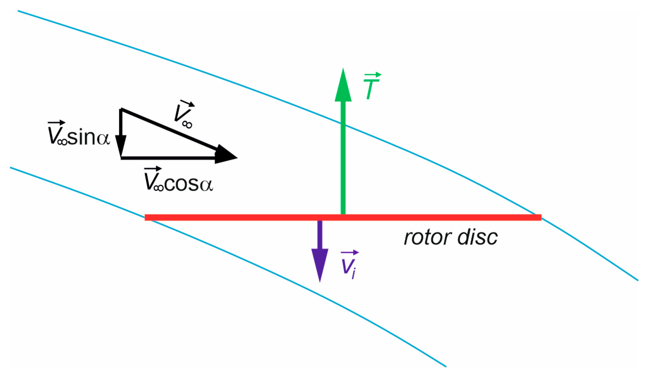
2. GIF Formulation and Solution Procedure

According to the momentum theory for forward flight (Figure 1), the GIF is a transcendent fixed-point equation for the induced inflow ratio:

$${\lambda }_i=\frac{C_T}{2\sqrt{{\mu }^2+{\left({\mu }_z+{\lambda }_i\right)}^2}},$$

(1)

which can be expressed in algebraic irrational zero-point form as

$${\lambda }_i-\frac{C_T}{2\sqrt{{\mu }^2+{\left({\mu }_z+{\lambda }_i\right)}^2}}=0,$$

(2)

and in rational (normal) form as follows

$$4{\lambda }_i^4+8\mu \tan {\alpha }_D{\lambda }_i^3+4{\mu }^2\left({\tan }^2{\alpha }_D+1\right){\lambda }_i^2-C_T^2=0.$$

(3)

Instead of the induced inflow ratio ${\lambda }_i$, the rotor inflow ratio $\lambda$ can be used as a variable in Equation (1):

$$\lambda ={\lambda }_i+{\mu }_z=\frac{C_T}{2\sqrt{{\mu }^2+{\lambda }^2}}+\mu \tan {\alpha }_D$$

(4)

with the algebraic zero-point irrational form given as

$$\lambda -\frac{C_T}{2\sqrt{{\mu }^2+{\lambda }^2}}-\mu \tan {\alpha }_D=0,$$

(5)

and rational form:

$$4{\lambda }^4-8\mu \tan {\alpha }_D{\lambda }^3+4{\mu }^2\left({\tan }^2{\alpha }_D+1\right){\lambda }^2-8{\mu }^3{\tan \alpha }_D\lambda +4{\mu }^4{\tan }^2{\alpha }_D-C_T^2=0.$$

(6)

Equations (3) and (6) are quartic algebraic equations that can be represented as

$${\mathrm{A}}_4{x}^4+{\mathrm{A}}_3{x}^3+{\mathrm{A}}_2{x}^2+{\mathrm{A}}_{1}x+{\mathrm{A}}_0=0.$$

(7)

Constants ${\mathrm{A}}_0{, \mathrm{A}}_1{, \mathrm{A}}_2{, \mathrm{A}}_3{, \mathrm{and} \mathrm{A}}_4$ are given in

Table 1. Coefficients of the GIF rational form.

Constant	$\mathbf{Variable} \mathit{x}={\mathit{\lambda }}_{\mathit{i}}$	$\mathbf{Variable} \mathit{x}=\mathit{\lambda }$
${\mathrm{A}}_4$	$4$	$4$
${\mathrm{A}}_3$	$8\mu {\tan \alpha }_D$	$- 8\mu {\tan \alpha }_D$
${\mathrm{A}}_2$	$4{\mu }^2\left({\tan }^2{\alpha }_D+1\right)$	$4{\mu }^2{(\tan }^2{\alpha }_D+1)$
${\mathrm{A}}_1$	$0$	$- 8{\mu }^3{\tan \alpha }_D$
${\mathrm{A}}_0$	$- C_T^2$	$4{\mu }^4{\tan }^2{\alpha }_D-C_T^2$

.

Equations (2) and (5) are irrational because they have an unknown in the radicand. Equations (3) and (6) represent their normal (rational) forms, respectively. Although no recommendation can be found in the literature dealing with the question of which GIF form is the best for numerical solving, there is a clear reason for preferring an irrational form. Namely, in addition to the roots of the original (irrational) form, the normal form may contain some superfluous roots that are not solutions of the original form [19]. On the other hand, the rational form is more suitable for calculating derivatives, which can be a significant factor if a one-point method of a high order of convergence is engaged to solve the equation. There are four forms of the GIF, which can be solved numerically, and Equations (2), (3), (5), and (6) represent them.

Procedures for numerical solving of GIF can be found in [20] (pp. 97–98) and [21] (pp. 126, 579–580). Both authors use the NR method to solve an irrational form for $\lambda$ (Equation (5)) and state that three-four iterations are sufficient in most cases. Leishman [20] suggests two numerical methods with practical engineering use: a simple fixed-point iteration (FPI) and NR method, where FPI typically requires 10–15 iterations, but in some cases, especially at lower advance ratios, a larger number of iterations may be necessary. For stopping criteria, the author uses an error estimator as follows:

$$\epsilon =\left|\frac{{\lambda }_{n+1}-{\lambda }_n}{{\lambda }_{n+1}}\right|,$$

(8)

and states that when $\epsilon \le 0.0005$ convergence is said to occur. According to Leishman, the initial value for ${\lambda }_0$ is usually the inflow ratio for hover:

$${\lambda }_h=\sqrt{C_T/2}.$$

(9)

W. Johnson [21,22] recommends the initial value for ${\lambda }_0$ as

$${\lambda }_{wj}=\frac{{\lambda }_h^2}{\sqrt{{\left({\lambda }_h+{\mu }_z\right)}^2+{\mu }^2}}+{\mu }_z.$$

(10)

In addition, the author proposes using a relaxation factor $r_f=0.5$ for convergence improvement:

$${\lambda }_{n+1}={\lambda }_n-r_f\frac{f\left(\lambda \right)}{f’\left(\lambda \right)}.$$

(11)

The initial value given in Equation (10) can be modified to become even closer to the root as

$${\lambda }_{md}=\frac{{\lambda }_h^2}{\sqrt{{\left({\lambda }_e+{\mu }_z\right)}^2+{\mu }^2}}+{\mu }_z,$$

(12)

where ${\lambda }_e$ is the main inflow ratio for edgewise flight (${\alpha }_D=0$):

$${\lambda }_e=\frac{1}{\sqrt{2}}\sqrt{\sqrt{{\mu }^4+4{\lambda }_h^4}-{\mu }^2}.$$

(13)

Next to the numerical solution for $\lambda$, the GIF can also be solved for ${\lambda }_i$. However, in the literature, no analysis compares the number of iterations and other parameters of the numerical solution for those two variables. Therefore, six initial guesses (values) for ${\lambda }_0$ are considered in this study, as it is shown in

Table 2. Initial guesses ${\lambda }_0$ for GIF numerical solutions.

Main Inflow Ratio $\mathit{\lambda }$ Equations (5) and (6)	Induced Inflow Ratio ${\mathit{\lambda }}_{\mathit{i}}$, Equations (2) and (3)	Reference
${\lambda }_h$	${\lambda }_h$	Leishman [20]
$\frac{{\lambda }_h^2}{\sqrt{{\left({\lambda }_h+{\mu }_z\right)}^2+{\mu }^2}}+{\mu }_z$	$\frac{{\lambda }_h^2}{\sqrt{{\left({\lambda }_h+{\mu }_z\right)}^2+{\mu }^2}}$	W. Johnson [15,16]
$\frac{{\lambda }_h^2}{\sqrt{{\left({\lambda }_e+{\mu }_z\right)}^2+{\mu }^2}}+{\mu }_z$	$\frac{{\lambda }_h^2}{\sqrt{{\left({\lambda }_e+{\mu }_z\right)}^2+{\mu }^2}}$	Current study

.

A few years ago, GIF’s analytical, closed-form solution was presented and offered to the rotorcraft community as a benchmark solution in helicopter aerodynamics for comparing numerical results [18]. It is a relatively new, easily programmable solution based on linear algebra and symbolic mathematics, with the potential to be used instead of numerical solving. Since the author examined only one case ($\mu =0.1$, $C_T=0.003$, ${\alpha }_D=4°$) with the primary pedagogical goal of demonstrating the power of novel mathematical tools, the analytical solution is not taken as a benchmark solution. However, it is evaluated, along with numerical methods.

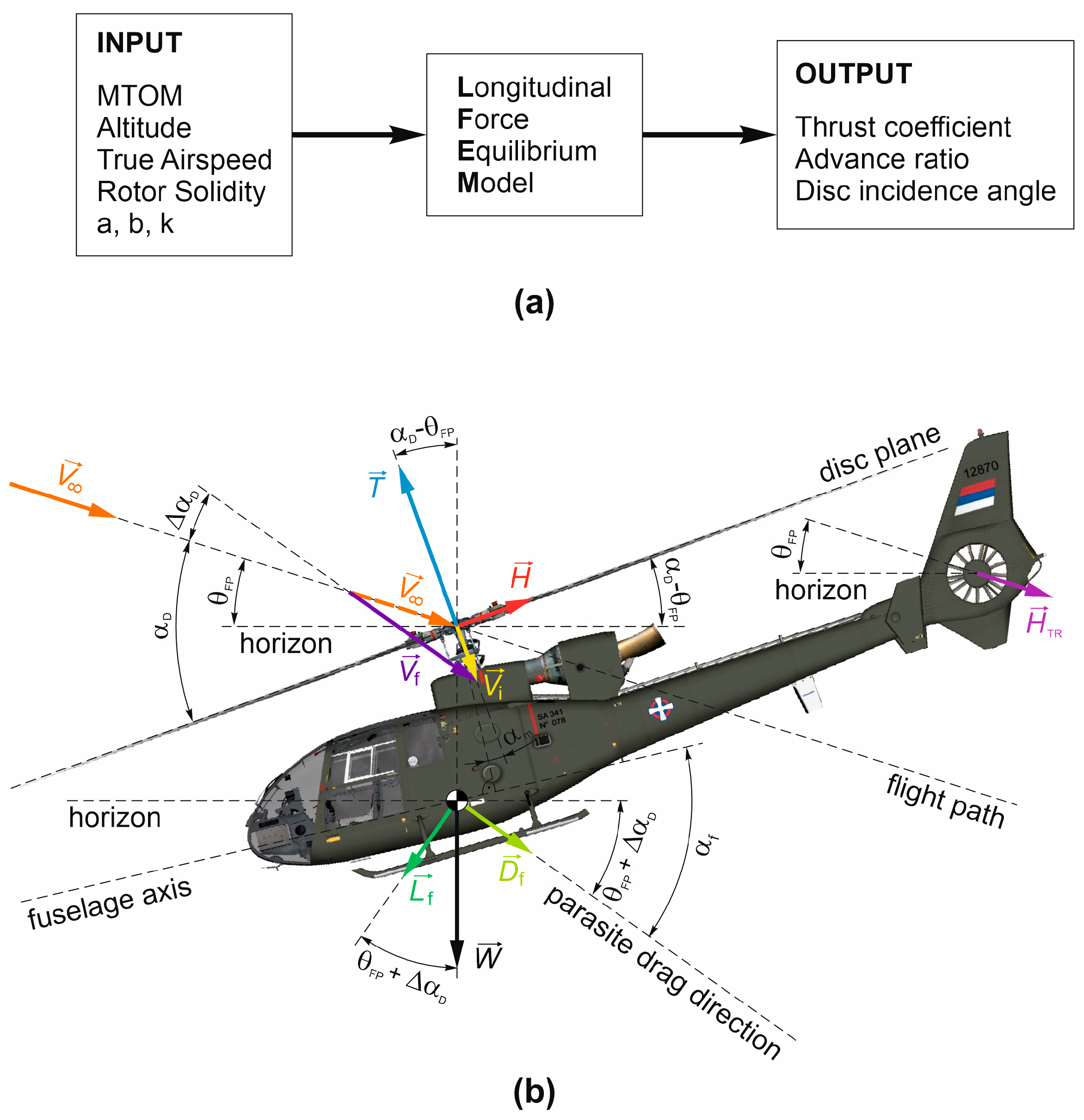
3. Models and Methods

GIF has only three parameters: advance ratio $\mu$, thrust coefficient $C_T$, and rotor disc incidence angle (angle of attack) ${\alpha }_D$. These parameters are mutually determined, and their ranges need to be defined. Only for this research, the union of all $\mu$, $C_T$, and ${\alpha }_D$ combinations that may occur in steady-level flight conditions are named the Acceptable Parameter Range (APR). It is a fictive union of all steady-level flight regimes of an infinite number of single-rotor helicopters that may exist in practice.

Accordingly, two tasks are imposed:

• Definition of a method for determining the APR;
• Presentation of the APR with a finite number of cases.

Precise determination of APR boundaries is a complex and time-consuming process requiring sophisticated and computationally demanding tools. The main goal is to exclude from the numerical analysis as many cases as possible that have no practical significance and to ensure that a potential conclusion about the use of a particular numerical method in solving the Glauert inflow equation refers to the widest possible ranges of steady-level flight conditions, take-off masses, geometric and aerodynamic characteristics of helicopters. Therefore, it is enough to use a robust, fast, and sufficiently reliable tool capable of providing that the APR boundaries it sets encompass all possible cases. For that reason, the following steps are adopted:

• Selection of a finite number of cases for APR boundaries determination purposes;
• Establishing the APR boundaries as $C_T{}_{min}=f_1\left(\mu \right)$, $C_T{}_{max}=f_2\left(\mu \right)$, ${\alpha }_D{}_{min}=f_4\left(\mu \right)$ and ${\alpha }_D{}_{max}=f_4\left(\mu \right)$;
• Establishing a more expansive APR zone with an acceptable safety margin;
• Determination of the finite number of possible cases as APR zone representatives for numerical methods evaluation purposes.

The range of possible cases is very wide. There are many ultralight RW-UAV applications and a few single-rotor helicopters with a maximum take-off mass (MTOM) below 300 kg. The MTOM of the largest helicopter in the world is greater than 50,000 kg. The Official World Record in the category Rotorcraft–Altitude in horizontal flight set above ISA troposphere boundary (11,010 m) by sky-crane helicopter Sikorsky CH-54B on 4 November 1971. The fastest helicopter in the world is the British Lynx, with an achieved forward flight speed of 400.87 km/h. The Lynx held this title for 37 years.

Considering the high variability in rotorcraft take-off mass, flight speed, altitude, and other characteristics, around 7 million points are selected and divided into four working groups (WG), as shown in

Table 3. Finite number of cases of Working (WG) and Control Groups (CG).

Characteristics		Group 1	Group 2	Group 3	Group 4
MTOMmin/Δm/MTOMmax 1	WG	1000/500/8500	9000/2000/19,000	20,000/5000/35,000	40,000/10,000/80,000
	CG	1000/200/8800	9000/400/19,600	20,000/800/40,000	41,600/1600/80,000
hmin/Δh/hmax		0/500/11,500
fe,max/fe,mean/fe,min		Calculated based on [21,22,23,24,25,26]
Vmin/ΔV/Vmax		1/1/131
σmin/σmean/σmax		0.04/0.01/0.2
amin/amax		130/150
bmin/bmax		0.85/1.15
kmin/kmax		0.39/1.35
No. of WG points		3,621,888	1,358,208	905,472	1,131,840
No. of CG points		32,823,360	22,155,768	21,335,184	20,514,600
Total No. of WG points:		7,017,408	Total No. of CG points:		96,828,912

¹ Three different TOM are used for each MTOM: empty, mean, and max (see the Julia^® LFEM code).

. The selection process is based on past and current design trends [21,22,23,24,25,26]. Next, the parameters a, b, and k are used to determine helicopter main and tail rotor diameter, angular velocity, and equivalent helicopter drag/lift area by statistics. Finally, the control group (CG) is used for grid density validation.

The first task in the APR establishing process is to develop an algorithm for GIF parameter determination. Considering the number of calculations that must be performed to determine the APR zone is measured in millions, a simplified approach to the problem of helicopter-trimmed flight is necessary. In this regard, only the longitudinal force equilibrium model (LFEM) is used, as shown in Figure 2.

LFEM is based on a simple low-fidelity longitudinal trim model given in [27] (pp. 116–118). The longitudinal force equilibrium equations for steady-level flight are:

$$T\sin ({\alpha }_D)+L_F\sin (\mathrm{\Delta }{\alpha }_D)-H_c{\cos }^2({\alpha }_D)-D\cos (\mathrm{\Delta }{\alpha }_D)-H_{TR}=0,$$

(14)

and

$$T\cos ({\alpha }_D)+H_c\sin ({\alpha }_D)\cos ({\alpha }_D)-W_{og}-L_f\cos (\mathrm{\Delta }{\alpha }_D)-D\sin (\mathrm{\Delta }{\alpha }_D)=0.$$

(15)

The lack of complete trim equations (longitudinal moment balance and lateral force and moment balance) results in a lower quality of the obtained solutions, which is compensated by increasing the safety margin of the established APR boundaries. Because of demanding computational requirements, flapping effects, rotor imperfections, and nonlinearities are also neglected.

On the other hand, usual small angle assumption, typical for simplified low-fidelity models, cannot be applied, which significantly complicates the mathematical model and increases the number of nonlinear equations that must be solved simultaneously. In addition, airframe lift force and tail rotor drag force are addressed. The solution is obtained in two steps: LFEM transformation into a single longitudinal force equilibrium equation (LFE) and numerical solution of LFE using the NR method. LFEM and its numerical solution procedure are described in detail in Appendix A.

3.1. Available Power Limit

Many real limitations may be included in the LFEM model. The most important are available power and dynamic stall (stall-flutter) limit. Available power is strongly limited and is represented by Equation (16) which is obtained by statistical data from [23]:

$$P_{TO}=0.0764W_{MTO}{}^{1.1455}, \left\{{\epsilon }_{av}=14\%, {\epsilon }_{MAX}=37\%, R_c=0.989, W_{MTO}\left[\mathrm{kg}\right]\right\}.$$

(16)

Since the maximum errors have always been on the side of overestimating the available power, the following expression is adopted for the maximum take-off power in [kW]:

$$P_{TO}=87.096W_{MTO}^{1.1455}.$$

(17)

For altitudes up to 4000 m, the adopted model gives that the maximum available power is 95% of the output engine(s) power. The remaining 5% covers the power needs of the tail rotor, other consumers, and transmission losses. Furthermore, the novel hybrid and fully electrical power units were not observed because of their much lower gravimetric power density than hydrocarbon fuel-based power plants. For higher altitudes, available power is represented as a function of static pressure and temperature ratio:

$$P_{A_{h>4000m}}=0.95P_{TO}\frac{\delta }{\sqrt{\theta }}.$$

(18)

On the other hand, the required power $P_R$ has been calculated using the following expression:

$$P_R=C_p\rho \pi R^2{V}_t^3,$$

(19)

where

$$C_p=k_i{\lambda }_i{C}_T+\frac{\sigma c_d}{8}{F}_p+\frac{1}{2}\frac{f_e}{\pi R^2}{\mu }_c^3.$$

(20)

The empirical factor $k_i$ considers blade tip losses, nonuniform inflow, and other rotor non-perfections, and is given in

Table 4. The rotor induced power empirical factor $k_i$.

$\mathit{\mu }$	${\mathit{k}}_{\mathit{i}}$	Reference
$0<\mu \le 1$	$1.15÷1.2$	Vast literature
$\mu \le 0.5$	$1.075\cosh \left(6.76{\mu }^2\right)$	[28]
$0.5<\mu \le 1$	$1.0-29.332\mu +92.439{\mu }^2-51.746{\mu }^3$
$\mu \le 0.2$	1.2	Current study
$0.2<\mu \le 0.4$	$2\mu +0.8$
$\mu >0.4$	$14\mu -4$

. The blade profile drag empirical factor $F_p$ with an error of less than 1% for all speed ranges was developed in [28] as

$$F_p=\sqrt{1+{\mu }_c^2}\left(1+\frac{5}{2}{\mu }_c^2+\frac{3}{8}{\mu }^2\frac{4+7{\mu }_c^2+4{\mu }_c^4}{{\left(1+{\mu }_c^2\right)}^2}-\frac{9}{16}\frac{{\mu }^4}{1+{\mu }_c^2}\right)+\left(\frac{3}{2}{\mu }_z^4+\frac{3}{2}{\mu }_z^2{\mu }^2+\frac{9}{16}{\mu }^4\right)\ln \frac{1+\sqrt{1+{\mu }_c^2}}{{\mu }_c},$$

(21)

and it is used in this study. In addition, as the small angle assumption is not employed, ${\mu }_c$ is used instead of $\mu$ in Equation (20).

3.2. Stall Flutter Limit

Dynamic stall is a phenomenon that allows the local angle of attack to grow beyond the static stall limit. Such conditions include high drag penalties, negative pitch damping, and amplified vibrations. Dynamic stall criteria usually represent a limit beyond which forward flight is unacceptable due to excessive pitch link vibrations, although the rotorcraft is usually still flyable. Many empirical dynamic stall models, such as the Boeing, ONERA, and the Leishman–Beddoes model, have been developed. These models are primarily used in complex rotary-wings modeling. On the other hand, F. Harris [29] developed simple stall criteria, which can be implemented in low-fidelity models:

$$\frac{C_T}{\sigma }=\frac{C_{l_{MAX}}}{6}\frac{1-{\mu }^2+\frac{9}{4}{\mu }^4}{1+\frac{8}{3}\mu +\frac{3}{2}{\mu }^2}$$

(22)

In this study, a simple assumption is made that the dynamic stall limit on the retreating blade is 50% greater than the static stall limit, and a slightly modified Harris criterion for a retreating blade stall at $0.75R$ is used as

$$C_{l_{rb}}<C_{l_{MA{X}_{rb,dynamic}}},$$

(23)

where

$$C_{l_{rb}}=C_{l_{av}}\frac{1+\frac{8}{3}\mu +3{\mu }^2+4{\mu }^3+\frac{9}{4}{\mu }^4}{1-{\mu }^2+\frac{9}{4}{\mu }^4}$$

(24)

The maximum lift coefficient at $0.75R$ of the retreating blade depends on local Reynolds and Mach numbers. For this study, the blade airfoil maximum lift capabilities are based on NACA 0012 airfoil, and the influence of the local Reynolds number is modeled as

$$C_{l_{MA{X}_{rb,static, M_{rb}<0.3}}}=67.57-34.07\log R_{e_{loc}}+5.722{\log }^2{R}_{e_{loc}}-0.3141{\log }^3{R}_{e_{loc}},$$

(25)

where the local Reynolds number is defined as

$$R_{e_{loc}}=\frac{\left(0.75V_t-V\cos \left({\alpha }_D\right)\right)·c}{\nu }$$

(26)

Equation (25) is obtained from [30] (Figure 13) by the GraphPad PRISM^® software tool for nonlinear regression analysis and is used if $3\times {10}^5\le R_{e_{loc}}\le 8\times {10}^6$. The maximum lift coefficient on the retreating blade for lower Reynolds numbers is set to 1.0 and for higher ones to 1.75. Furthermore, the influence of the Mach number is also obtained from [30] (Figure 14) similarly:

$$C_{l_{MA{X}_{rb,static, M_{rb}>0.3}}}=-\frac{C_{l_{MA{X}_{rb, static}}}}{0.8}{M}_r+1.1\frac{C_{l_{MA{X}_{rb, static}}}}{0.8}$$

(27)

The maximum static lift coefficient $C_{l_{MA{X}_{\left(av, stat,\right)}}}$ can be calculated by Equations (25) and (27) where $M$ and $R_e$ are used instead of $M_r$ and $R_{e_{loc}}$.

3.3. Numerical Methods and Procedures

This subsection presents two computational plans: a plan for APR boundary determination and a GIF numerical solution with certain numerical methods. In this regard, The Numerical Computation Plan 1 for APR determination is shown in

Table 5. Numerical Computational Plan 1 (NCP 1).

Cycle No.	Group	Model	Cycle No.	Group	Model
1.	WG 1–4	No limit	5.	WG 1–4	Power 2 limit
2.	WG 1–4	Power limit	6.	WG 1–4	Power 3 limit
3.	WG 1–4	Dynamic stall	7.	CG 1–4	No limit
4.	WG 1–4	Power 1 limit

. There are seven cycles of calculations: 6 cycles refer to 4 working groups (WG 1–4), and the last refers to 4 control groups (CG 1–4), as presented in Table 3. The control groups are introduced to check the influence of the grid density on the obtained results. In total, over 2.5 billion LFE calculations were performed. This demanding and computationally expensive task has been completed on a workstation with 20 processor cores. The computational code is written in the Julia^® programming language because it is one of the best solutions for large-scale numerical work [31].

As can be seen in Table 5, there are three Power limits models. The Power 1 model is described in the previous subsection. Power 3 is practically the same, with the difference that the small angle assumption is adopted, which means that Equation (20) contains $\mu$. Finally, Power 2 model uses the classic Gessow and Crim approach to the compressibility effect on the blade profile drag. The main task of this model is to serve as a benchmark for the Power 1 limit model.

In this paper, GIF is first numerically solved by a three-point eight-order Sharma-Sharma (Sharma) method using multi-precision numerical computing. The Sharma method is robust and helpful for single and multiple root-finding problems that require only four functional evaluations [32]. A high level of accuracy is obtained by the Arb.Numerics Julia^® package for arbitrary precision, which is set to 200 of the 2500 available significant digits. Numerical computing of GIF in this research is performed with the:

• Standard arithmetic precision;
• Arbitrary arithmetic precisions (only for the benchmark solution);
• Initial values are taken from Table (2);
• Stopping criteria$E_o<\epsilon$ ($\epsilon =5\times {10}^{-n}, n=4, 6, 8, 10, 12, 16$) or “one iteration”;
• Stopping criteria$E_o<5\times {10}^{-150}$ (only for the benchmark solution);
• Several one-point and multipoint iterative methods without memory for solving nonlinear equations.

The methods used are shown in

Table 6. GIF Numerical Computing Plan (NCP 2).

Methods	Type	Stopping Criteria	Equations	$\mathbf{Initial} \mathbf{Guesses} {\mathit{\lambda }}_{\mathit{o}}$
Halley	1P3R	$\epsilon <5\times {10}^{-4}$	Equation (6)	${\lambda }_h$
Chebyshev	1P3R	$\epsilon <5\times {10}^{-6}$	Equation (5)	${\lambda }_{wj}$
Kiss	1P4R	$\epsilon <5\times {10}^{-8}$	Equation (3)	${\lambda }_{md}$
E5	1P5R	$\epsilon <5\times {10}^{-10}$	Equation (2)
NR	1P2R	$\epsilon <5\times {10}^{-12}$
NR with f = 0.5	-	$\epsilon <5\times {10}^{-14}$
Ostrowski	2P4R	$\epsilon <5\times {10}^{-16}$
Chun	2P4R	1 iteration
Cordero	2P4R
Jarratt	2P4R
Sharma–Sharma	3P8R
BWR	3P8R
BWR II	3P8R
KT	3P8R

and thoroughly presented in [9,10,11]. As seen, 14 methods, 8 stopping criteria, 4 GIF forms, and 6 initial values were used, and 1344 numerical cycles were performed. Each cycle consists of about 3 million individual cases. For this work, GIF has been solved numerically about four billion times. The main goal of these numerical calculations is to obtain the following:

• Maximum, minimum, and average iteration number (ITNumb) as a function of $\mu$ for the entire APR.
• Maximum real relative error (E_t) for all examined cases;
• Percentage of cases of failed convergence, if any;
• Presence of non-physical roots;
• Quality assessment of used initial values;
• Quality assessment of iterative methods.

In addition to the above, it is essential to point out that each numerical method used in this research is written in the Julia^® programming language in such a way that the iterative sequence will be interrupted in the case the stopping criteria are satisfied or the number of iterations is greater than 1000 (failed convergence) or the solution is a NaN, zero or infinite. While the acceptable solution is practically impossible to obtain in the case of failed convergence, in other cases (NaN, zero, or infinitive), the value from the previous iteration may be taken as a solution. Additionally, for multipoint methods, a solution from the previous step (point) of the same iteration may be delivered as a final. Consequently, if some multipoint method is used, the number of iterations (ITNumb) does not necessarily have to be an integer.

4. Results and Discussion

Firstly, the results of the APR determination are shown and discussed. Then, the following analysis of the performance of the selected numerical methods for solving the GIF whose parameters are in the APR is presented.

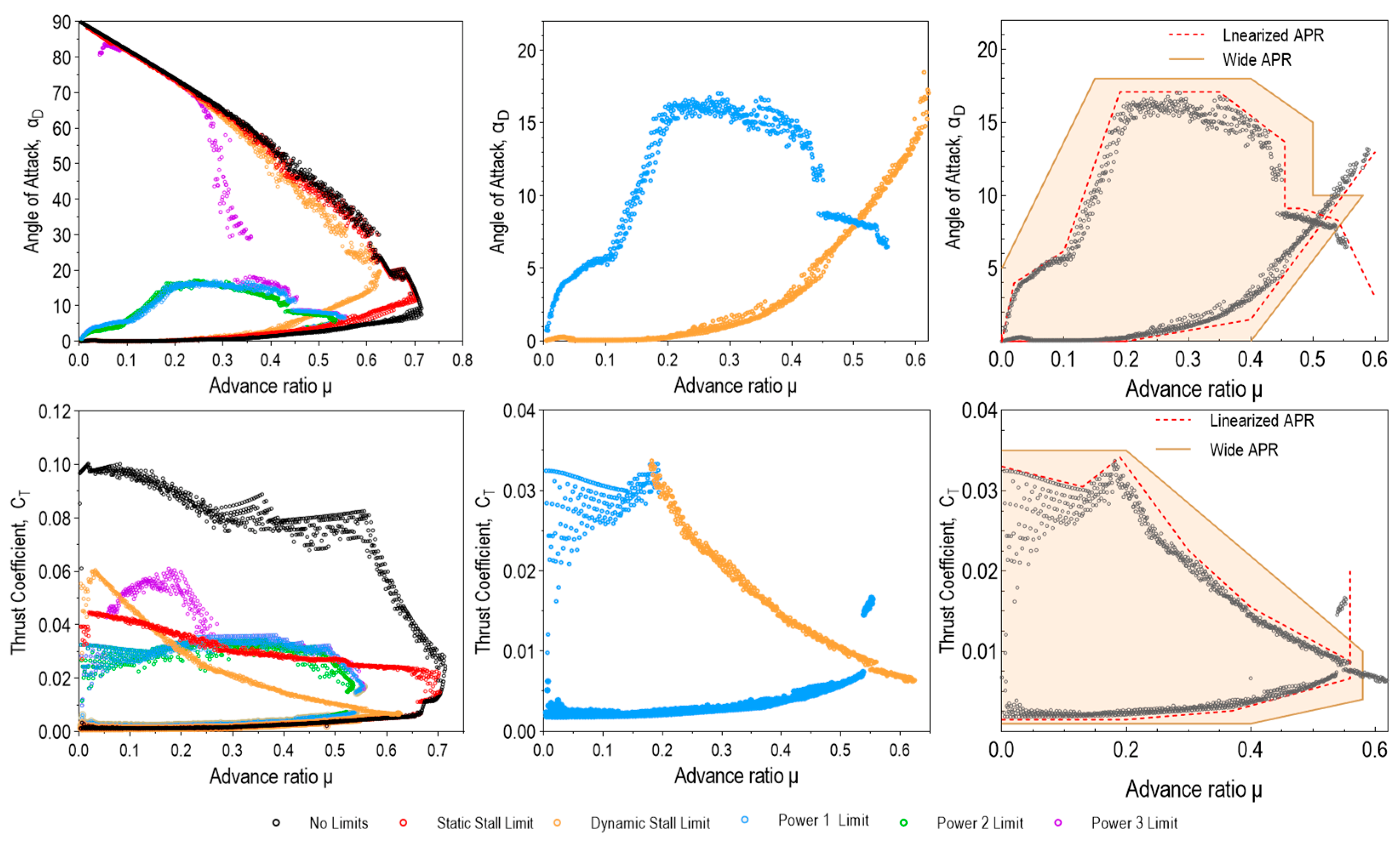
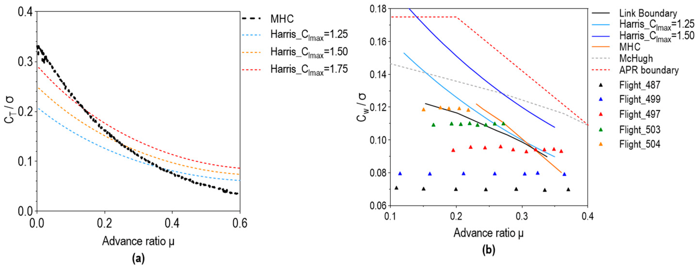
4.1. APR Determination

Figure 3 (left) shows the maximum and minimum values of the angle of attack and thrust coefficient for the basic LFE model (No limits) and five additional models with limits. As can be seen, maximum ${\alpha }_D$ values are restricted by Power 1 and Power 2 models. Furthermore, the matching of minimum and maximum values of $C_t$ and ${\alpha }_D$ which are obtained by these two models is excellent. However, the results obtained by Power 3 model compared to the previous two models deviate significantly in obtaining very large $C_t$ and ${\alpha }_D$ maximums for $0.05\le \mu \le 0.27$ and $0.04\le \mu \le$0.36, respectively. Minimum values of these parameters are very similar for all three Power models, while in comparison to them, the other three models give lower $C_{T_{min}}$.

Regarding $C_{T_{max}}$, for an advance ratio less than 0.2, the limit is provided by Power 1 model. In contrast, the emergence of dynamic stalling represents the main limiting factor for higher advance ratios. According to the above, the results obtained using Dynamic stall and Power 1 limits served as the basis for establishing the APR boundaries, shown in Figure 3 (middle). Because the very simple longitudinal force equilibrium model is used as an APR solver, a more expansive APR zone is established, as shown in Figure 3 (right). Grid density is verified by the control group, with about 97 million points. As presented in Figure S1, there are no significant differences between the working and control groups.

The main goal of LFEM is to determine the APR zone, and in this regard, a dynamic stall (stall flutter) limit is fundamental, especially for an advance ratio higher than 0.2. Unlike fixed-wing aircraft, rotorcraft normally fly in mild and medium stall flutter conditions because the blades very quickly leave the retreating side of the rotor. The main consequence of stall flutter is a pitch link vibratory load often used for practical stall boundary determination. As already mentioned, a modified Harris criterion (MHC) is used in this study. Figure 4a shows MHC obtained by NCP 1 execution compared to standard Harris criteria.

The data from [33] are used and compared with the MHC line adapted to the given helicopter model and test flight conditions for validation. As shown in Figure 4b, there is a relatively good matching of MHC with the pitch link vibratory limit. The advantage of such a modification on the Harris criterion is that it allows variability of the maximum lift coefficient depending on the local (representative) Reynolds and Mach numbers on the retreating blade, which is the place of stall flutter occurrence.

4.2. GIF Numerical Analysis

The results of the NCP 2 execution are given in this subsection. As previously stated, 1344 cycles were conducted, and each cycle had $N_{tot.}=4,375,561$ points. Given that one cycle requires solving the equation twice, GIF has been solved almost 11.8 billion times for regular and benchmark solutions. Due to the large number of obtained data, only the most important results are presented and discussed.

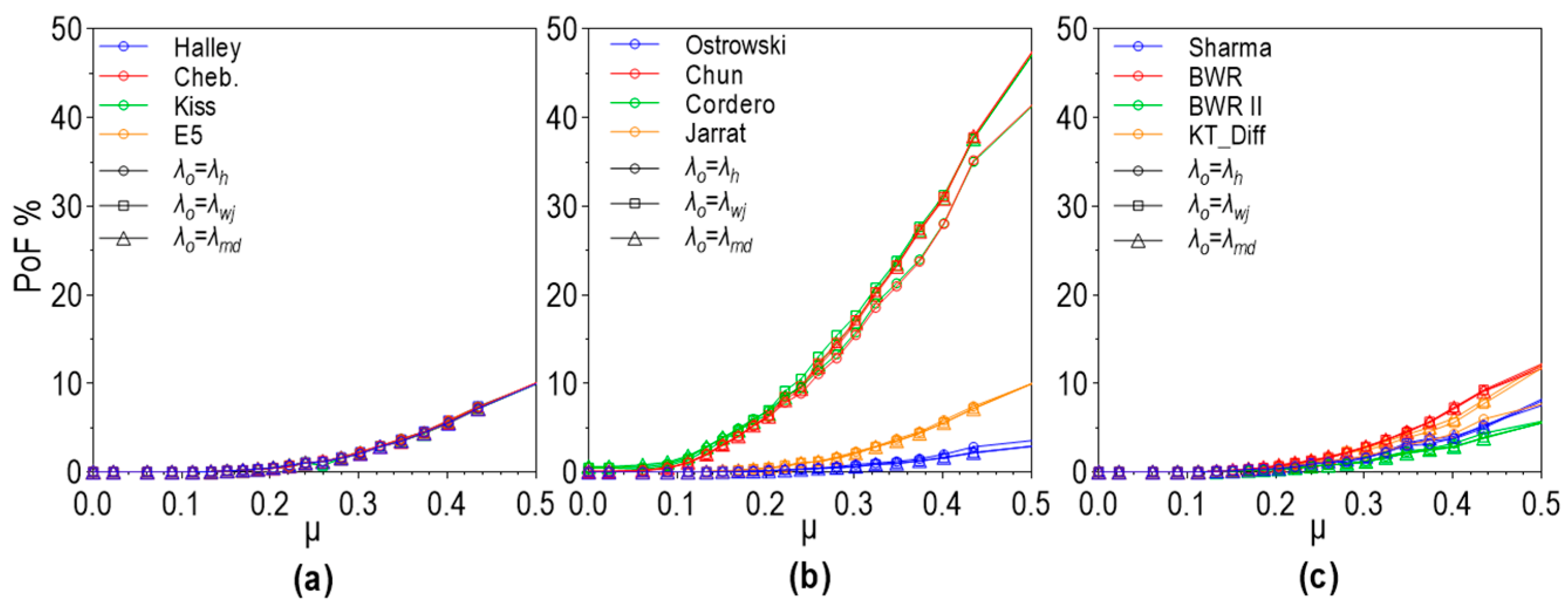
4.2.1. Percentage of Failed Convergence (PoF)

Iteration and failed convergence counters are built into the Julia^® code for all used numerical methods. The number of iterations greater than 1000 is empirically chosen to stop the solver and to indicate the occurrence of failed convergence. Firstly, numerical solutions of Equation (6) are examined. According to the results shown in

Table 7. Percentage of Failed Convergence, PoF (%), $\epsilon =5\times {10}^{-n}$, Equation (6).

${\lambda }_0$	n	One-Point Methods				Two-Point Methods				Three-Point Methods
		Halley	Chebyshev	Kiss	E5	Ostrowski	Chun	Cordero	Jarrat	Sharma	BWR	BWR II	KT Diff
${\lambda }_h$	16	2.16	2.15	2.15	2.15	0.76	12.39	12.84	2.15	1.62	2.68	1.28	1.75
	14	0	0	0	0	1 × 10−4	6 × 10−3	6 × 10−3	0	0.015	0	0.037	0.04
	12	0	0	0	0	0	0	0	0	2 × 10−4	0	0.024	0.002
	10	0	0	0	0	0	0	0	0	0	0	0.017	0
	8	0	0	0	0	0	0	0	0	0	0	1.2 × 10−4	0
	6	0	0	0	0	0	0	0	0	0	0	5.9 × 10−5	0
	4	0	0	0	0	0	0	0	0	0	0	9.8 × 10−6	0
${\lambda }_{wj}$	16	2.12	2.08	2.10	2.11	0.63	13.69	14.13	2.1	1.68	2.71	1.20	2.37
	14	0	0	0	0	5 × 10−5	5 × 10−3	5 × 10−3	0	0.012	0	0.05	0.032
	12	0	0	0	0	0	0	0	0	5 × 10−5	0	0.024	0.002
	10	0	0	0	0	0	0	0	0	0	0	0.07	2 × 10−5
	8	0	0	0	0	0	0	0	0	0	0	0.0015	0
	6	0	0	0	0	0	0	0	0	0	0	7.3 × 10−6	0
	4	0	0	0	0	0	0	0	0	0	0	3 × 10−6	0
${\lambda }_m$	16	2.11	2.11	2.11	2.11	0.64	13.60	13.95	2.1	1.77	2.69	1.21	2.55
	14	0	0	0	0	5 × 10−5	4 × 10−3	3 × 10−3	0	0.008	0	0.04	0.033
	12	0	0	0	0	0	0	0	0	7 × 10−5	0	0.032	0.001
	10	0	0	0	0	0	0	0	0	0	0	0.027	2 × 10−5
	8	0	0	0	0	0	0	0	0	0	0	0.0223	0
	6	0	0	0	0	0	0	0	0	0	0	1.3 × 10−4	0
	4	0	0	0	0	0	0	0	0	0	0	10−5	0

, the presence of failed convergence correlates with stopping criteria (required accuracy). Therefore, eliminating failed convergence presence by reducing the required accuracy is possible with all methods except the BWR II. In general, a small number of cases of failed convergence ($\mathrm{NoF}$) concerning the total number of performed calculations $N_{tot.}$. The percentage of failed convergence ($PoF$) is calculated as

$$PoF=100\frac{NoF}{N_{tot.}} \left[\%\right],$$

(28)

and its distribution over the advance ratio is shown in Figure 5. It can be seen that $\mathrm{PoF}$ increases with the advance ratio and reaches a value of around 50 percent for the Chun and Cordero methods. In addition, an initial value does not generally significantly influence the PoF. Finally, it is essential to note that using arbitrary precision in the Sharma method to calculate benchmark solutions has completely eradicated convergence failures. Since the double-precision floating-point arithmetic is set by default for real numbers in 64-bit system architecture (Float64), the maximum number of significant digits is about 15 to 17. Therefore, the accumulation of computational error is the probable cause of these failures.

To confirm this assumption, the case of the largest percentage of failed convergence from Table 7 ($\mathrm{PoF}=14.13\%, \epsilon =5\times {10}^{-16}, {\lambda }_o={\lambda }_{wj}$, Cordero method) was taken and recalculated with appreciably increased arithmetic precision. The ArbNumerics Julia^® package was used with 200 significant digits. As a result, the convergence was completely successful ($\mathrm{PoF}=0\%$). The same result was achieved using the BWR II method, where the failures were present for all stopping criteria.

Equation (3) has much better properties regarding convergence failures, as shown in

Table 8. Percentage of Failed Convergence, PoF (%), $\epsilon =5\times {10}^{-n}$, Equation (3).

${\lambda }_0$	n	Two-Point Methods				Three-Point Methods
		Ostr.	Chun	Cord.	Jarr.	Sh.Sh.	BWR	BWR II	KT
${\lambda }_h$	16	0.003	0.095	0.628	0	0	0	0.0015	0.0015
	14	0	0	0	0	0	0	0	0
${\lambda }_{wj}$	16	0.006	0.118	0.771	0	0	0	0.0021	0.001
	14	0	0	0	0	0	0	0	0
${\lambda }_{md}$	16	0.006	0.087	0.571	0	0	0	0.0028	0.0015
	14	0	0	0	0	0	0	0	0

. One-point methods are not presented in the table because no failures were detected for $\epsilon <1\times {10}^{-17}$. When it comes to multipoint methods, there are certainly cases of convergence failures, but only if $\epsilon \ge 1\times {10}^{-16}$. Equations (2) and (5) express excellent properties: no cases of failed convergence were found for declared precision.

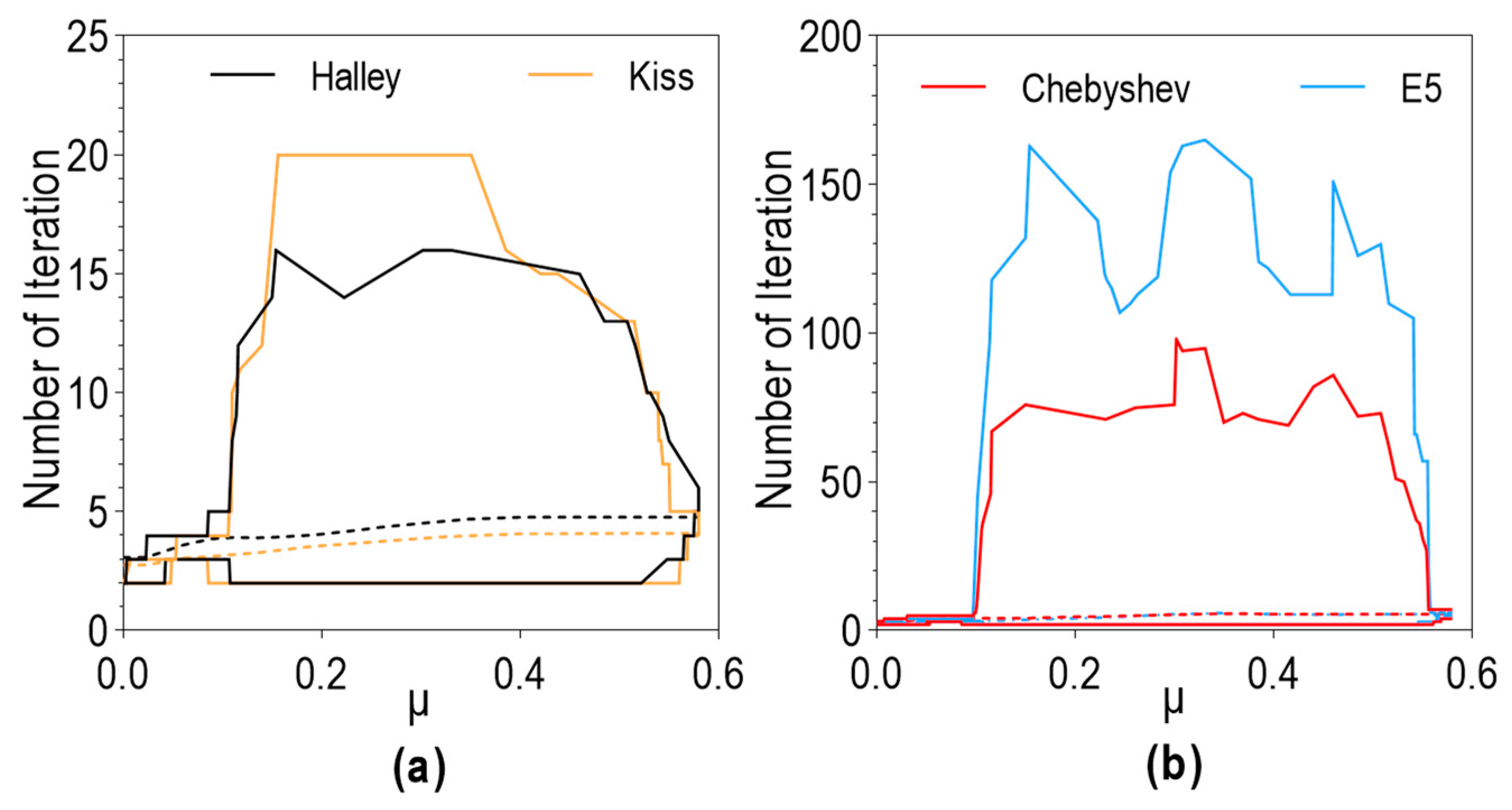
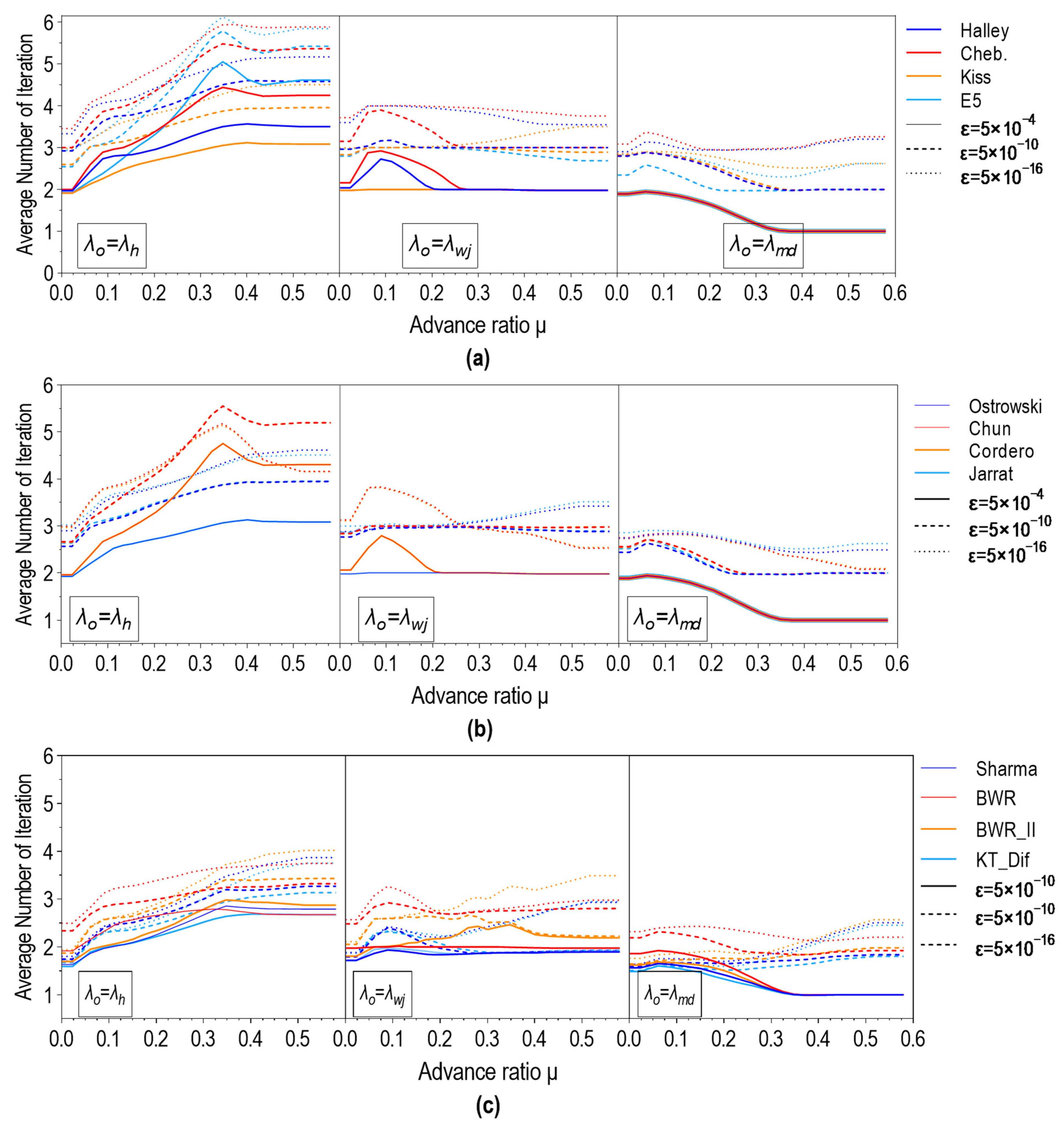
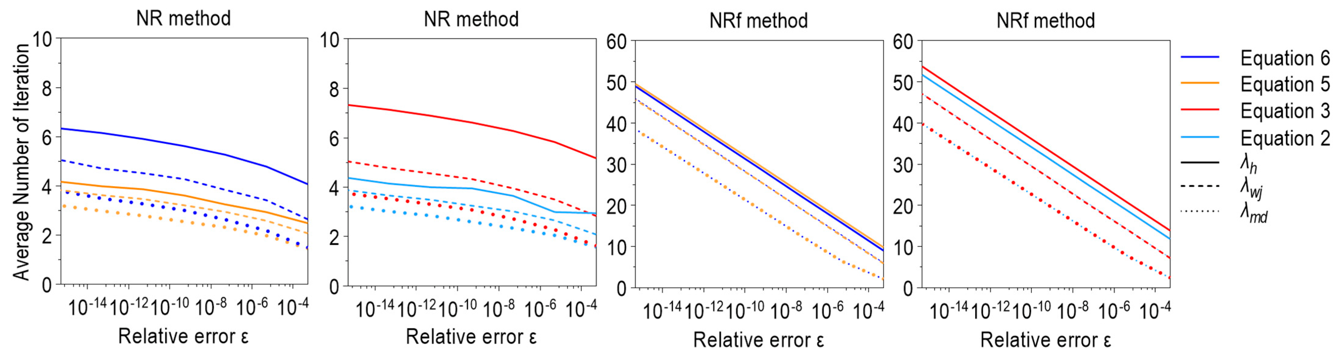
4.2.2. Number of Iterations (ITNumb)

As in the previous subsection, Equation (6) was analyzed first. Figure 6 shows the number of iterations of one-point methods for an initial guess ${\lambda }_0={\lambda }_h$ and stopping criteria $\epsilon =5\times {10}^{-14}$. The maximum number of iterations is relatively large and reaches over 150 for the E5 method and over 15 iterations for the Halley and Kiss methods. The minimum number of iterations ranges from two to three. The average $ITNumb$ is about four iterations for all one-point methods and is represented by dashed lines on two diagrams in Figure 6.

The total number of cases in which the required number of iterations is greater than 10 ranges from 0.02 to 4.15 percent, and three to five iterations are sufficient in 87.5 to 97.5% of cases, depending on the chosen one-point method. The results (ITNumb vs. advance ratio) for other stopping criteria ($\epsilon =5\times {10}^{-n}, n=4, 6, 8, 10, 12, 16$) and for multipoint methods (where ${\lambda }_0={\lambda }_h$) are very similar to the above (Figure 6).

The required number of iterations can be drastically reduced if ${\lambda }_{wj}$ or ${\lambda }_{md}$ are used instead of ${\lambda }_h$, as shown in Figure 7. The stopping criteria are essential because a small $\epsilon$ (high-required accuracy) causes a larger number of iterations. As can be seen in Figure S2, only one iteration in about 75% and up to two iterations in 99.8% of cases is sufficient if the Sharma method is used in conjunction with ${\lambda }_0={\lambda }_{md}$, where stopping criteria are set on $\epsilon =5\times {10}^{-14}$.

Even better results are obtained if the irrational form is solved. Namely, under the same conditions, Equation (5) is solved with the Sharma method in two or fewer iterations in all cases. Figures S3–S8 show an average number of iterations and their percentage distribution of remaining GIF forms. As can be seen, the use of improved, i.e., modified initial value (${\lambda }_{md}$) significantly reduces the required number of iterations, regardless of the stopping criteria, the type of method used, and the form of the Equation being solved.

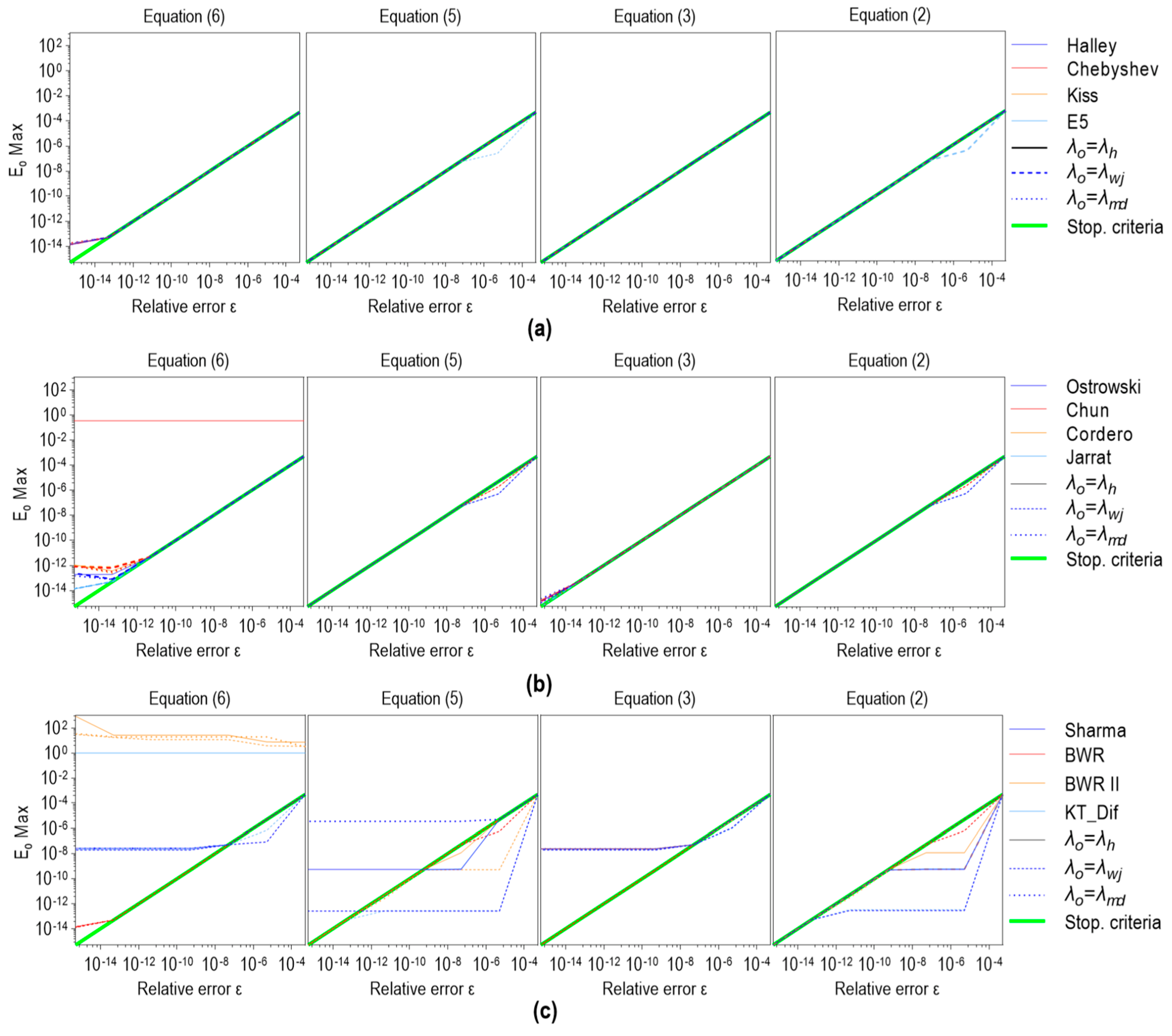
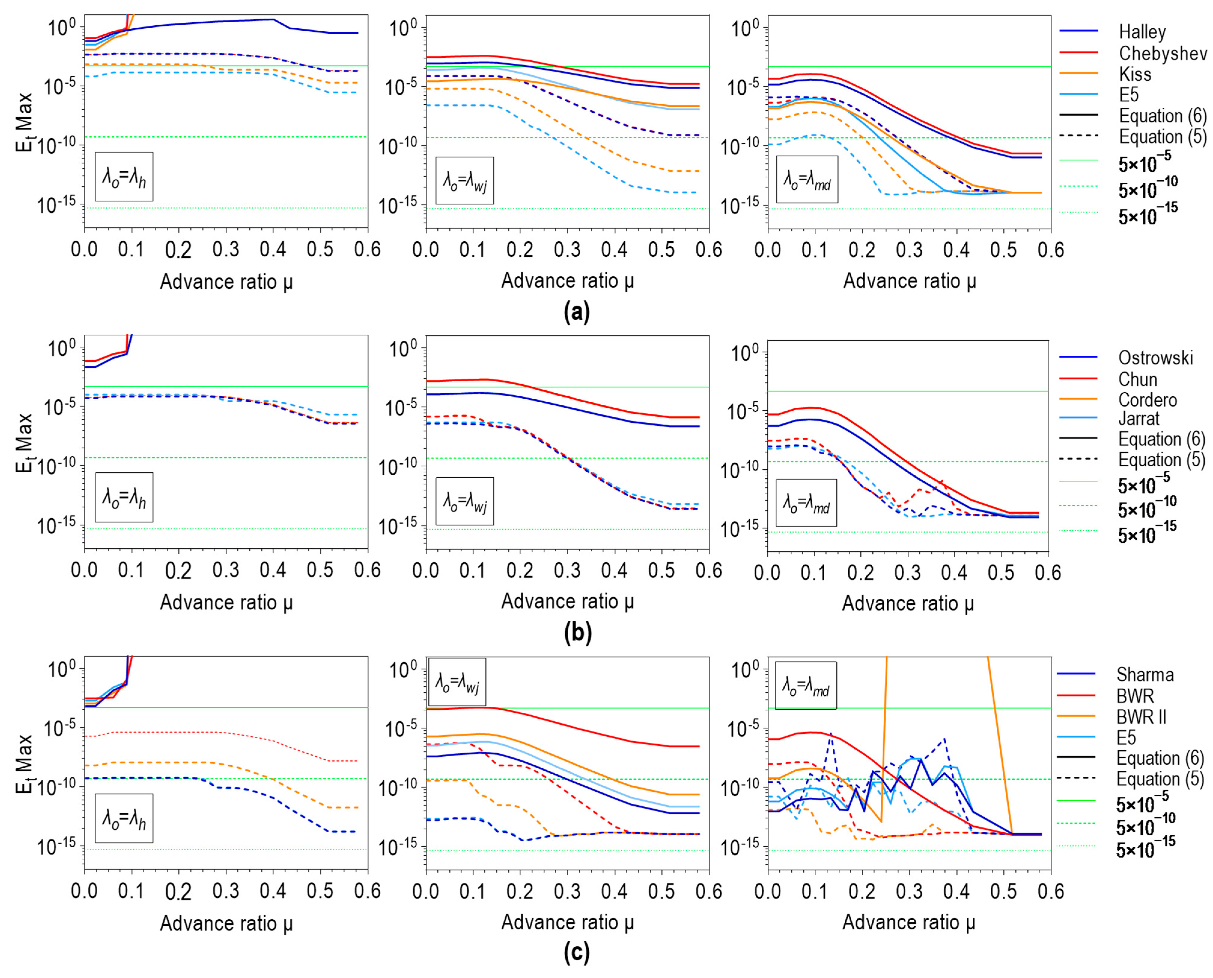
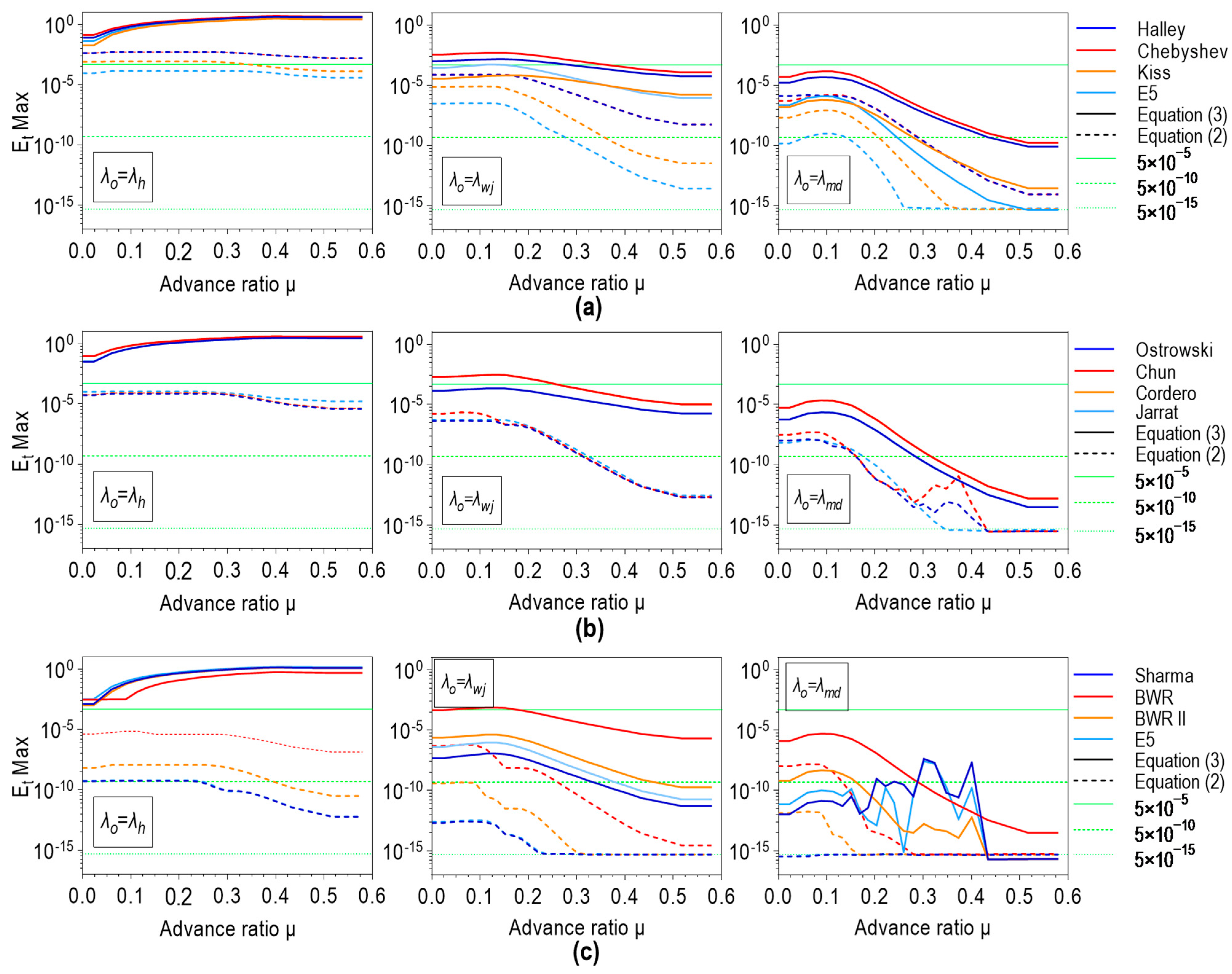
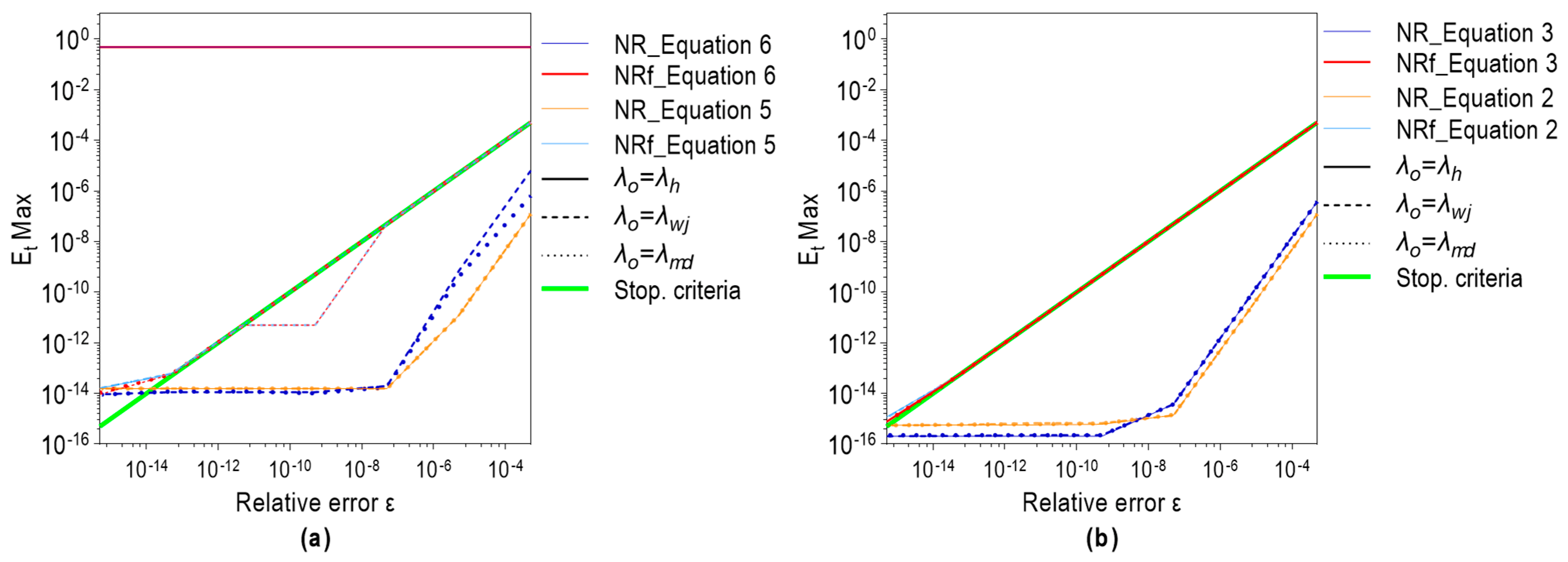
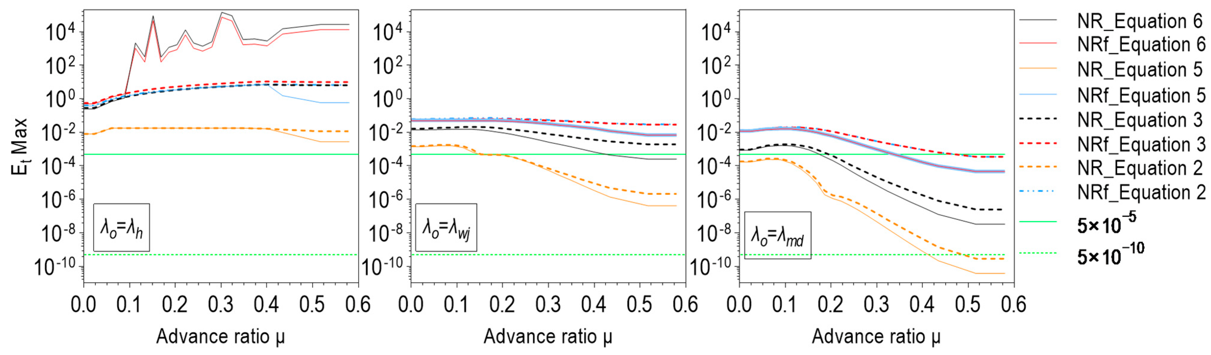
4.2.3. Relative Errors ($E_o$, $E_t$)

Let ${\lambda }_{HPS}$ be the benchmark solution of GIF obtained using high precision with 200 significant digits. Then, $E_t$ is a relative error with respect to the benchmark solution

$$E_t=\left|\frac{{\lambda }_f-{\lambda }_{HPS}}{{\lambda }_{HPS}}\right|,$$

(29)

where ${\lambda }_f$ is a final numerical solution reached using a standard computational precision of up to approximately 16 significant digits. As a reminder, the relative input error that was used as a stopping criterion in the iterative cycle is marked with $\epsilon$ and defined by Equation (8). It represents the maximum acceptable relative distance between two adjacent solutions in the iterative sequence. The relative output error is defined as

$$E_o=\left|\frac{{\lambda }_f-{\lambda }_{f-i}}{{\lambda }_f}\right|,$$

(30)

where ${\lambda }_{f-i}$ is a solution from the previous iteration ($i=1$) or the previous point of the same iteration step ($i\in \left\{1/3, 1/2, 2/3\right\}$, applicable only to multipoint methods).

According to the above, all analyzed numerical methods come to the solution in two ways:

• $E_o<\epsilon$—an iterative process is accomplished, convergence is achieved, the input criterion is fulfilled, and the output solution is ${\lambda }_f$;
• $E_o\ge \epsilon$—the stopping criterion is not activated, but the iterative process is interrupted due to the failed convergence or due to an inappropriate solution (NaN, infinite, or zero). Then, ${\lambda }_{f-i}$ becomes a final numerical solution ${\lambda }_f$.
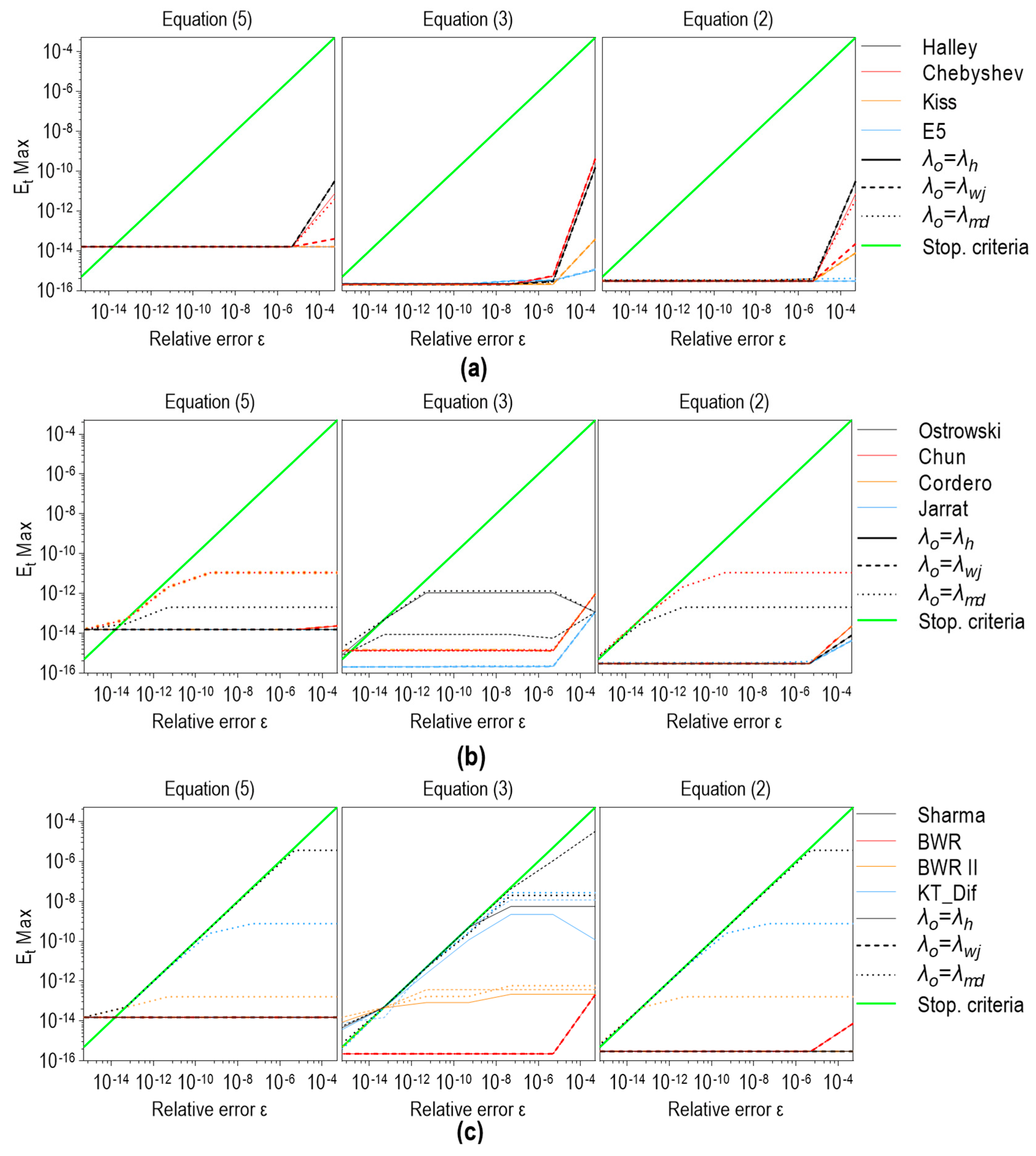
• The first case ($E_o<\epsilon$) can be seen in the following diagrams in Figure 8;
• Equation (6), all methods, all initial values;
• Equations (2), (3), and (5), one-point methods, all initial values;
• Equation (3), two-point methods, all initial values.

Anomalies can be observed on other charts ($E_o\ge \epsilon$). The occurrence of failed convergence has already been discussed, and a comparative analysis of data shown in Table 7 and Table 8 with the charts in Figure 8 leads to the two groups of anomalies whose cause is different from convergence failure. The first group refers to Equation (6) solved by:

• Chun and KT Diff, which gives $E_o{}_{max}\approx 1$ for all stopping criteria where ${\lambda }_0={\lambda }_h$;
• KT Diff with ${\lambda }_0\in \left\{{\lambda }_{wj},{\lambda }_{md}\right\}$, which gives $E_o{}_{max}\approx 2.5\times {10}^{-8}$ $\left\{\epsilon <{10}^{-8}\right\}$;
• Sharma with ${\lambda }_0\in \left\{{\lambda }_h,{\lambda }_{wj},{\lambda }_{md}\right\}$, which gives $E_o{}_{max}\approx 2.5\times {10}^{-8}$ for $\epsilon <{10}^{-8}$.

The second group includes Equations (3) and (5) solved by the Sharma method with ${\lambda }_0\in \left\{{\lambda }_h, {\lambda }_{wj}, {\lambda }_{md}\right\}$, which also give $E_o{}_{max}>\epsilon$, as shown in Figure 8. The most common cause of anomalies is NaN, which does not necessarily represent an unfavorable outcome. For example, when finding a benchmark solution, NaN occurs in 100% of cases, but ${\lambda }_{f-i}$ is already a sufficiently high-quality solution after $1+i$ iterations, and in that case, $E_o{}_{max}\approx 5\times {10}^{-51}$. The total maximum varies with the change in advance ratio, as shown in Figure 9. The same applies to the spectrum of $E_o{}_{max}$ values given in Figure 8, while their dependence on the advance ratio is shown in Figures S9–S12.

Given that the subject of the study is the examination of numerical methods with standard accuracy (up to 16–17 digits), it is much more essential to analyze maximum relative errors compared to the benchmark solution ($E_{t_{max}}$), which are given in Figure 10 and Figure 11. Figure 10 shows $E_{t_{max}}$ for all methods and initial values used in solving Equations (2), (3), and (5). As can be seen, the actual minimal accuracy (the maximal error) $E_{t_{max}}$ is far better compared to the stopping criteria $\epsilon$ and the maximal output relative error $E_{o_{max}}$. However, when it comes to Equations (3) and (5), it is noted that $E_t\ge \epsilon$ but only for the highest required precision ($\epsilon =5\times {10}^{-16}$). Furthermore, the lowest accuracy is detected for the Sharma method used with ${\lambda }_0={\lambda }_{md}$ in all three equations, which is explained by the small number of iterations and the high order of convergence of the method.

Figure 11 shows $E_{t_{max}}$ for Equation (6). These results are presented separately from Figure 10 because they require a more detailed analysis. Namely, all one-point methods used in conjunction with ${\lambda }_h$ indicate that $E_{t_{max}}\approx 0.5$ regardless of stopping criteria. The same applies to all two-point methods except the Chun and the three-point Sharma and BWR methods. With omitted methods, the results are even worse (extremely high values of $E_{t_{max}}$), but they are easily explained. It is enough to look at the corresponding diagrams in Figure 8 and see that anomalies ($E_o{}_{max}\gg \epsilon$) have already been detected there.

Additionally, BWR II methods have a high maximal actual relative error ($4\times {10}^2<E_o{}_{max}<5\times {10}^8$) for all initial values, but it is clear that this phenomenon is a consequence of failed convergence. Completely satisfied stopping criteria with excellent output relative error on the one side and disappointingly large actual relative error on the other can only be explained only by a successful convergence to superfluous roots, which is the case.

Further analysis revealed superfluous roots are always at a distance$\left|\mathrm{\Delta }\lambda \right|\ge 0.0035$ from the physical solution. This fact enabled the calculation of the probability of convergence towards the “wrong” solution during solving Equation (6). Figure 12 shows that probability increases with the advance ratio and reaches over 60 percent. It should be noted again that this applies only to ${\lambda }_0={\lambda }_h$, which is essential considering that using ${\lambda }_h$ as an initial value is standard practice. Equation (3) also represents a rational form of the inflow equation, but the “superfluous roots” problem was not detected.

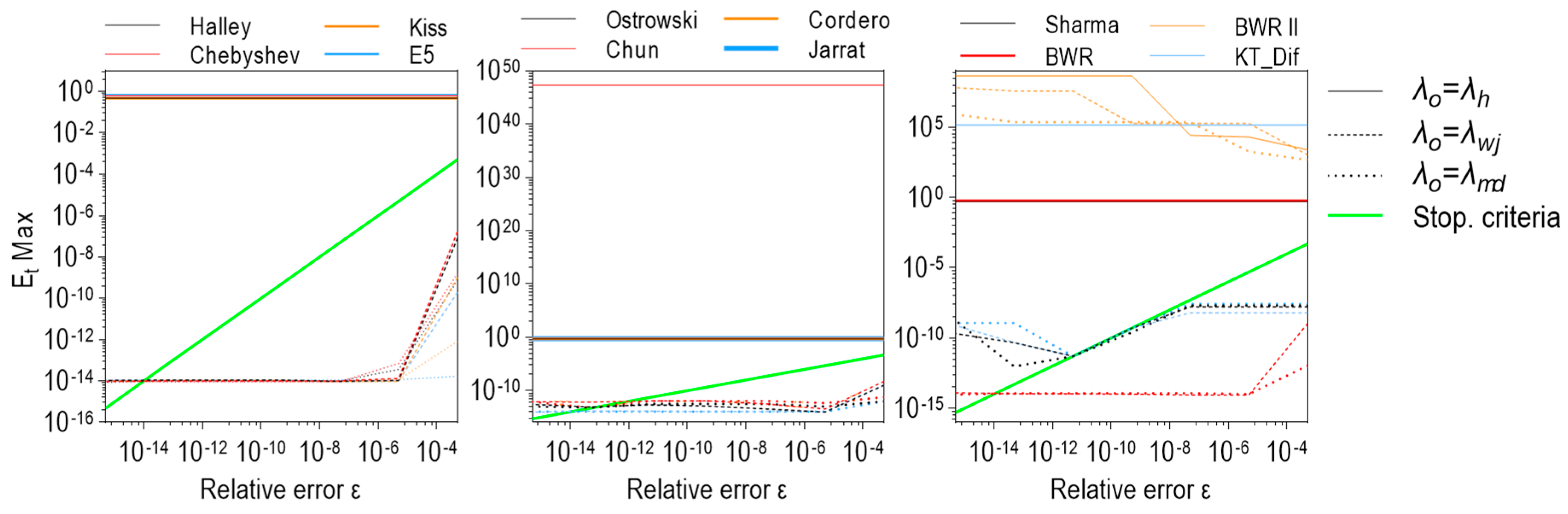
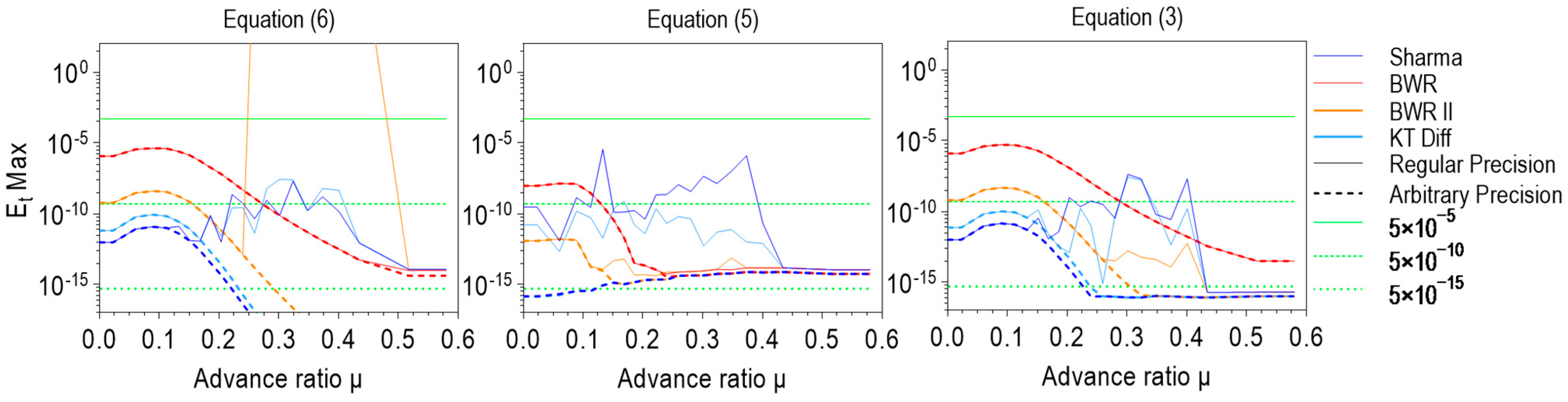
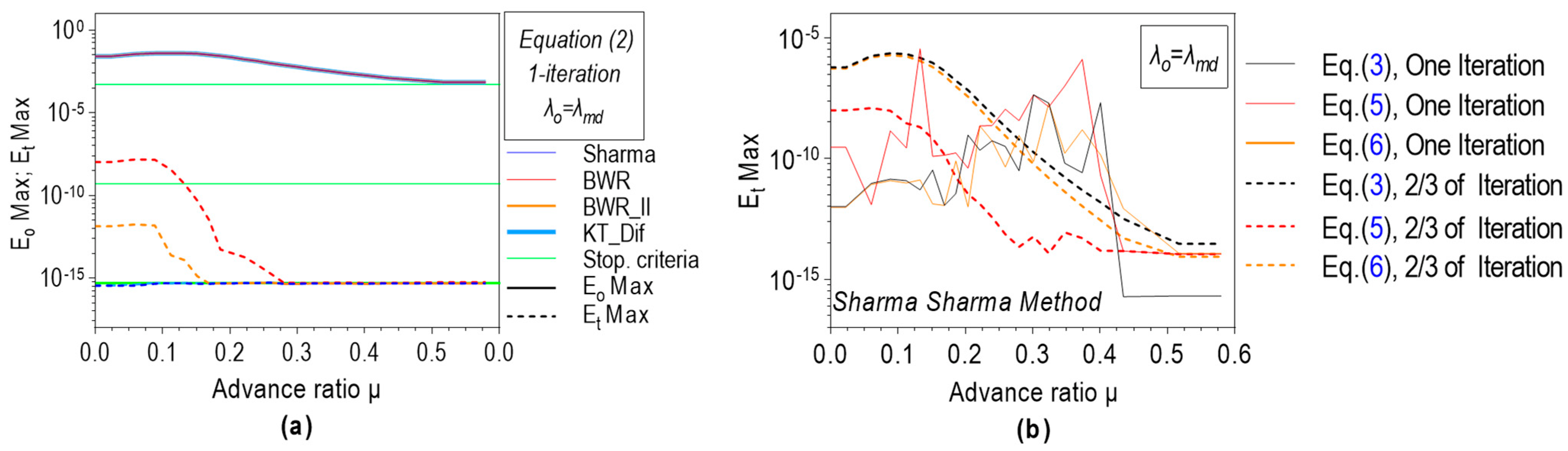
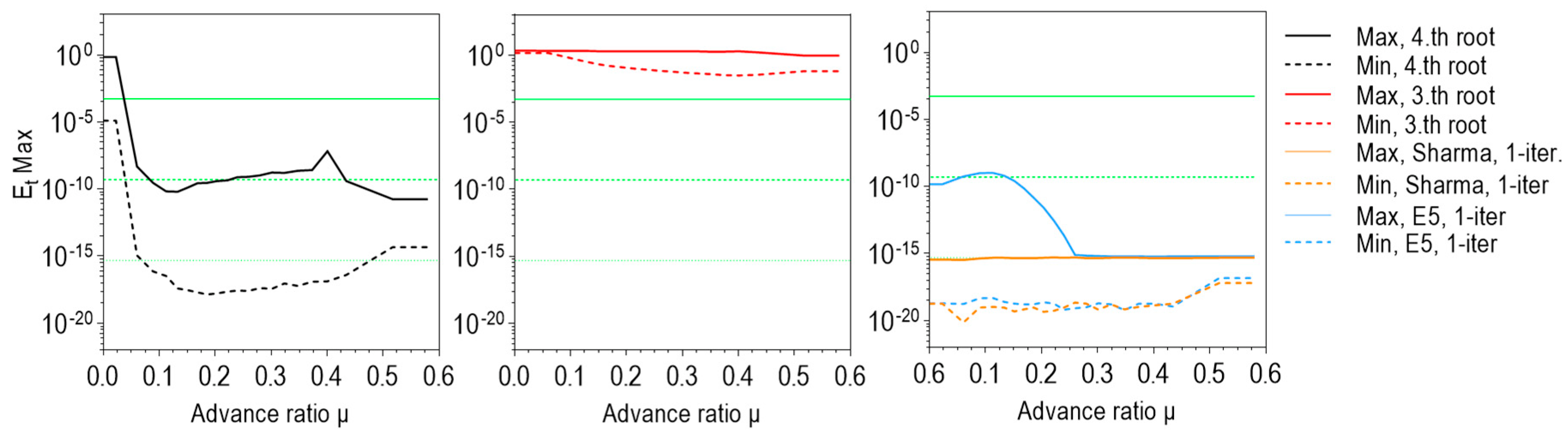
4.2.4. One Iteration Solution

A solution obtained in just one iteration can be considered noniterative in the practical sense because stopping criteria are not used. Figure 13 and Figure 14 show maximal relative error with respect to the benchmark solution, depending on the advanced ratio $\mu$ for Equations (5), (6) and (2), (3), respectively. After analyzing these charts, several findings can be highlighted:

• Convergence towards an extraneous root may occur if ${\lambda }_h$ is used as an initial value to solve Equation (6), regardless of chosen method;
• The solutions of Equation (3) obtained in one iteration with ${\lambda }_o={\lambda }_h$ has no practical significance regardless of the chosen method due to the very large maximal relative error concerning the benchmark solution ($E_{t_{max}}$);
• Failed convergence may occur if the BWR II method and ${\lambda }_{md}$ initial value are used to solve Equation (6) with standard arithmetic precision;
• Some anomalies in $E_{t_{max}}$ magnitude may appear if multipoint methods and ${\lambda }_{md}$ are used together to solve all forms of GIF except Equation (2), where no anomalies;
• $\left|E_t Max\right|<5.3\times {10}^{-16}$ is certainly reached over the entire range of advance ratio if the Sharma or KT Diff method is used in conjunction with ${\lambda }_{md}$ to solve Equation (2) which applies to standard arithmetic precision architecture. Figure S13 shows that the above conclusion applies only to the APR zone, i.e., that the numerical methods have worse performance outside the above zone;
• E5 one-point method used with ${\lambda }_o={\lambda }_{md}$ to solve Equations (2) and (3) provides high accuracy of obtained solution where $\left|E_t Max\right|<9.7\times {10}^{-10}$ for low advance ratios and $\left|E_t Max\right|<2.5\times {10}^{-14}$ for $\mu >0.23$.

The previously mentioned failed convergence, which occurs if the BWR II/${\lambda }_{md}$ pair is engaged in solving Equation (6) in standard precision, can be eliminated by using arbitrary precision with 200 significant digits, as shown in Figure 15. The same applies to the anomalies in $E_{t_{max}}$ magnitude that arise when some analyzed multipoint methods are used with ${\lambda }_o={\lambda }_{md}$ for numerical solving of all GIF forms except Equation (2), shown in Figure 15. Furthermore, it can be concluded that the accumulation of computational error at standard precision affects the final accuracy of the obtained solution even after one iteration. The situation is even more unfavorable if multipoint methods are used in several iterations, which could already be seen in the previous subsection. The reason lies in the large difference between $E_o$ and $E_t$ after the first iteration (Figure 16a), which practically unnecessarily activates the second one. As a result, calculation error accumulates, and the final solution has less precision than one obtained after the first iteration.

For example, the numerical solving of Equation (5) by the Sharma method with an initial value ${\lambda }_o={\lambda }_h$ and stopping criteria $\epsilon \le 5\times {10}^{-8}$ always gives $\mathrm{ITNumb}=1.67$ and occurrence of NaN in 100% of cases, which means that the stopping criteria are not fulfilled, as is seen in Figure 8.

Computational error accumulates even during the first iteration, especially if the high order of convergence methods is used with the most precise initial value (${\lambda }_{md}$). In that regard, Figure 16b gives a comparative view of the maximal relative errors after the first iteration and after 2/3 of the first iteration for Sharma/${\lambda }_{md}$ duo used in solving Equations (3), (5), and (6). As can be seen, better precision is obtained after the first two steps compared to the whole iteration.

4.2.5. Newton–Raphson Method

The NR method, as the most commonly used tool for solving nonlinear equations, is analyzed separately due to its outstanding historical significance. It has been applied to solve all GIF forms with three initial values (${\lambda }_h, {\lambda }_{wj}, {\lambda }_{md}$), with or without the use of the convergence acceleration factor ($f=0.5$) recommended by W. Johnson in [21]. Regarding failed convergence, the NR method behaves similarly to the previously discussed one-point methods: it only occurs with Equation (6) in about two percent of examined cases. The relaxation factor reduces the number of convergence failures by about 7.5 times, as seen in Table S1. On the other side, using the relaxation factor $f=0.5$ significantly increases the number of iterations, which is presented in Figure 17. The maximum values of the required number of iterations are higher than the average and are shown in Figure S14. The maximum number of iterations of the NR method is at the level of examined one-point methods or even slightly higher. At the same time, the introduction of the relaxation factor significantly increases the number of required iterations. It does not apply to the case of solving Equation (6) with ${\lambda }_h$, where the maximum number of iterations is large for all methods.

Figure 18 shows the change in $E_{t_{Max}}$ depending on the stopping criteria $\epsilon$ for all GIF forms. As in previous cases, convergence towards extraneous roots is noticeable for Equation (6) and initial value ${\lambda }_h$. The positive influence of the relaxation factor $f=0.5$ in increasing the accuracy of the numerical solution is not detected. The relative error is higher or at least the same if the mentioned factor is used. In general, the relative accuracy of the numerical solution achieved by the NR method is at the level of the previously analyzed one-point methods.

The solution obtained in one iteration is shown in Figure 19. If the results are compared with the diagrams given in Figure 13a and Figure 14a, it can be concluded that the NR method does not perform better than other one-point methods in case of use in one iteration. In addition, Figure 19 shows the negative influence of the relaxation factor on the achieved accuracy.

4.3. GIF Analytical Solution

According to [18], an analytical solution gives four roots: one complex conjugate pair and two real roots. Unlike [18], where only one case (point) was considered, in this study, a closed-form solution is tested over the entire APR zone in 436,067,402 points, and the observations are as follows:

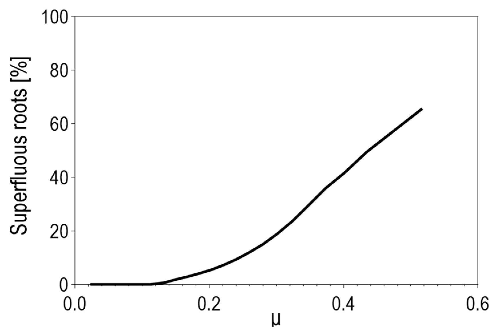
• The first two roots form a complex conjugate pair in 100% of tested cases and can be completely rejected;
• The third and fourth roots form a complex conjugate pair in 2.8% of tested points;
• The third and fourth roots are a NaN in 1.25% of cases;
• The third root is a negative real number in 49.6% of cases;
• If it is not a NaN or complex number, the fourth root represents a physical solution;
• The analytical solution is found in about 95% of the tested cases.

The accuracy of the analytical solution is shown in Figure 20. As can be seen, it has a much larger relative error, minimum and maximum, compared to very precise, previously analyzed numerical solutions obtained in only one iteration using the Sharma and E5 methods with an initial value ${\lambda }_0={\lambda }_{md}$ for solving Equation (2). The above, as well as the fact that a solution cannot be found in about five percent of cases, leads to the conclusion that closed-form solution does not show sufficient quality in comparison with numerical methods.

4.4. GIF Computational Cost

In order to complete the comparison of multipoint with single-point methods, it is necessary to evaluate the computational cost of the applied methods. Furthermore, verifying whether the multipoint method will achieve its computational efficiency in practice is necessary. In a limited numerical experiment applied to the rational forms of GIF, by comparing the time required for identical calculations on a sample of over 21.4 million different combinations of GIF parameters, the comparative advantage of the three-point methods was confirmed. Introducing an additional four-point method (order of convergence equal to 16) showed that these methods have the weakest performance of all analyzed methods. Therefore, three-point methods represent the optimal choice. In addition, introducing the relaxation factor in the NR method increases the required calculation time compared to the standard method by about 50 percent. The selected initial guess and stopping criteria have an impact on the required calculation time, but to a much lesser extent than the choice of the method itself. The KT Diff method stands out for its calculation speed. The obtained results are shown in Table S2 and given in the Supplementary Material (https://github.com/marjanvtsl/GIF-Numerical-Analysis.git, accessed on 23 February 2023).

5. Conclusions and Recommendations

Symbolic algebra, arbitrary-precision arithmetics, and multipoint numerical methods are proficient mathematical tools used in engineering practice. They allow old, entrenched methods to be replaced by more modern, faster, and efficient ones. The low-fidelity longitudinal force equilibrium model of a single-rotor helicopter in forward flight is modified (no small angle assumption) and represented by one nonlinear variable equation instead of a system of nonlinear equations, which significantly simplifies the numerical solution procedure. The used algorithm allows changing the variant of the equation during the iterative cycle. Further practical implementation of the LFEM requires complete trim equations to be included in the model.

Regarding the numerical analysis of the GIF solution, the conclusions are as follows:

• The use of ${\lambda }_{wj}$ for the numerical solution of the Glauert inflow equation results in a smaller number of iterations and a higher accuracy of the obtained solution compared to the case when the induced ratio in hover ${\lambda }_h$ is used as an initial guess;
• Modifying the previously mentioned initial value (${\lambda }_{md}$) gives an even better result: the smallest average number of iterations and the highest precision of the solution regardless of the used method and stopping criteria;
• The chosen form of the Glauert inflow equation (rational or irrational, with unknown $\mathsf{\lambda }$ or ${\mathsf{\lambda }}_{\mathrm{i}}$) directly affects the performance of the numerical solution where the best convergence failure-free performance gives Equation (2);
• Optimal three-point methods used along with ${\lambda }_{md}$ and high accuracy requested often lead to anomalies that significantly degrade the performance of the used method, and in this regard, it is much better to use them in only one iteration procedure for standard precision arithmetic;
• Multi-precision arithmetic is computationally expensive, but it completely frees the solutions from the accompanying anomalies;
• Analytical solutions in the standard arithmetic precision environment perform much worse than numerical solutions;
• The Sharma–Sharma, KT Diff, and optionally E5 methods, used in only one iteration, with ${\lambda }_{md}$ as an initial value for induced inflow ratio in solving Equation (2), have all attributes to become methods of choice for solving the GIF for a single-rotor helicopter in steady-level flight conditions below dynamic stall limit.

References

- Glauert, H. The Theory of the Autogyro. J. R. Aeronaut. Soc. 1927, 31, 483–508. [Google Scholar] [CrossRef]
- Peters, D.A. How Dynamic Inflow Survives in the Competitive World of Rotorcraft Aerodynamics. J. Am. Helicopter Soc. 2009, 54, 011001. [Google Scholar] [CrossRef] [Green Version]
- Smith, M.J.; Moushegian, A. Dual-Solver Hybrid Computational Approaches for Design and Analysis of Vertical Lift Vehicles. Aeronaut. J. 2022, 126, 187–208. [Google Scholar] [CrossRef]
- Chen, R.T. A survey of nonuniform inflow models for rotorcraft flight dynamics and control applications. In Proceedings of the Fifteenth European Rotorcraft Forum, Amsterdam, The Netherland, 12–15 September 1989. [Google Scholar]
- Peters, D.A.; Modarres, M.; Howard, A.B.; Rahming, B. A Third Approximation to Glauert’s Momentum Theory. J. Am. Helicopter Soc. 2016, 61, 042007. [Google Scholar] [CrossRef]
- Rubin, R.L.; Zhao, D. New Development of Classical Actuator Disk Model for Propellers at Incidence. AIAA J. 2021, 59, 1040–1054. [Google Scholar] [CrossRef]
- Petrovic, Z.; Stupar, S.; Kostic, I.; Simonovic, A. Determination of a Light Helicopter Flight Performance at the Preliminary Design Stage. Stroj. Vestn. J. Mech. Eng. 2010, 56, 535–543. [Google Scholar]
- Traub, J.F. Iterative Methods for the Solution of Equations, 2nd ed.; Chelsea Publishing Company: New York, NY, USA, 1982. [Google Scholar]
- Petkovic, M.S.; Neta, B.; Petkovic, L.; Dzunic, J. Multipoint Methods for Solving Nonlinear Equations, 1st ed.; Elsevier Science Publishing Co., Inc.: San Diego, CA, USA, 2014; ISBN 9780123972989. [Google Scholar]
- Dzunic, J. Multipoint Methods for Solving Nonlinear Equations. Ph.D. Thesis, University of Nis, Nis, Serbia, 2012. [Google Scholar]
- Petkovic, M.S.; Neta, B.; Petkovic, L.; Dzunic, J. Multipoint methods for solving nonlinear equations: A survey. Appl. Math. Comput. 2014, 226, 635–660. [Google Scholar] [CrossRef] [Green Version]
- Berahas, A.S.; Jahani, M.; Richtárik, P.; Takáč, M. Quasi-Newton methods for machine learning: Forget the past, just sample. Optim. Methods Softw. 2022, 37, 1668–1704. [Google Scholar] [CrossRef]
- Goldfarb, D.; Ren, Y.; Bahamou, A. Practical quasi-newton methods for training deep neural networks. Adv. Neural Inf. Process. Syst. 2020, 33, 2386–2396. [Google Scholar] [CrossRef]
- Davis, K.; Schulte, M.; Uekermann, B. Enhancing Quasi-Newton Acceleration for Fluid-Structure Interaction. Math. Comput. Appl. 2022, 27, 40. [Google Scholar] [CrossRef]
- Bogaers, A.E.J.; Kok, S.; Reddy, B.D.; Franz, T. Quasi-Newton methods for implicit black-box FSI coupling. Comput. Methods Appl. Mech. Eng. 2014, 279, 113–132. [Google Scholar] [CrossRef] [Green Version]
- Akbari, A.; Giannacopoulos, D. An efficient multi-threaded Newton–Raphson algorithm for strong coupling modeling of multi-physics problems. Comput. Phys. Commun. 2021, 258, 107563. [Google Scholar] [CrossRef]
- Liu, L.; Zhang, H.; Wu, Y.; Liu, B.; Guo, J.; Li, F. A modified JFNK with line search method for solving k-eigenvalue neutronics problems with thermal-hydraulics feedback. Nucl. Eng. Technol. 2023, 55, 310–323. [Google Scholar] [CrossRef]
- Ganguli, R.A. Pedagogical Example for STEM Using the Glauert Inflow Equation, Mathematica and Python. In Proceedings of the AIAA SciTech Forum, San Diego, CA, USA, 7–11 January 2019. [Google Scholar] [CrossRef]
- Bronshtein, I.N.; Semendyayev, K.A.; Musiol, G.; Muehlig, H. Handbook of Mathematics, 5th ed.; Springer: Berlin/Heidelberg, Germany, 2007; ISBN 978-3-540-72121-5. [Google Scholar]
- Leishman, G.J. Principles of Helicopter Aerodynamics, 2nd ed.; Cambridge University Press: Cambridge, UK, 2006. [Google Scholar]
- Johnson, W. Rotorcraft Aeromechanics; Cambridge University Press: New York, NY, USA, 2013. [Google Scholar]
- Johnson, W. NDARC—NASA Design and Analysis of Rotorcraft: Theory; Appendix 3, Release 1.11; TP–2015-218751; National Aeronautics and Space Administration: Washington, DC, USA, 2016.
- Rand, O.; Khromov, V. Helicopter Sizing by Statistics. J. Am. Helicopter Soc. 2004, 49, 300–317. [Google Scholar] [CrossRef]
- Harris, F.D. Introduction to Autogyros, Helicopters, and Other V/STOL Aircraft, Volume II: Helicopters; National Aeronautics and Space Administration: Washington, DC, USA, 2012.
- Prouty, R. Helicopter Performance, Stability and Control, 2nd ed.; Krieger Publishing Company: Malabar, FL, USA, 2002. [Google Scholar]
- Keys, C.N.; Wiesner, R. Guidelines for Reducing Helicopter Parasite Drag; Boeing Vertol Company: Ridley Park, PA, USA, 1974. [Google Scholar]
- Bramwell, A.R.S.; Done, G.; Balmford, D. Bramwell’s Helicopter Dynamics, 2nd ed.; Butterworth-Heinemann: Oxford, UK, 2000. [Google Scholar]
- Harris, F.D. Rotor Performance at High Advance Ratio: Theory versus Test; NASA/CR-2008-215370; National Aeronautics and Space Administration: Washington, DC, USA, 2008.
- Harris, F.D. Rotary Wing Aerodynamics—Historical Perspective and Important Issues. In Proceedings of the American Helicopter Society National Specialist’s Meeting on Aerodynamics and Aeroacoustics, Arlington, TX, USA, 25–27 February 1987. [Google Scholar]
- McCroskey, W.J. A Critical Assessment of Wind Tunnel Results for the NACA 0012 Airfoil; NASA-TM-100019; National Aeronautics and Space Administration: Washington, DC, USA, 1987.
- Bezanson, J.; Edelman, A.; Karpinski, S.; Shah, V.B. Julia: A Fresh Approach to Numerical Computing. SIAM Rev. 2017, 59, 65–98. [Google Scholar] [CrossRef] [Green Version]
- Sharma, J.R.; Sharma, R. A new family of modified Ostrowski’s methods with accelerated eighth order convergence. Numer. Algor. 2010, 54, 445–458. [Google Scholar] [CrossRef]
- Lau, B.H.; Louie, A.W.; Griffiths, N.; Sotiriou, C.P. Performance and Rotor Loads Measurements of the Lynx XZ170 Helicopter with Rectangular Blades; NASA-TM-104000; National Aeronautics and Space Administration: Washington, DC, USA, 1993.
- Dodic, M.; Krstic, B.B.; Rasuo, B.P. Single Rotor Helicopter Parasite Drag Estimation in the Preliminary Design Stage. Tehnika 2018, 73, 65–77. [Google Scholar] [CrossRef] [Green Version]
- Bailey, F.J., Jr. A Simplified Theoretical Method of Determining the Characteristics of a Lifting Rotor in Forward Flight; NACA Report 716; US Government Printing Office: Washington, DC, USA, 1941.
- Lau, B.H.; Louie, A.W.; Griffiths, N.; Sotiriou, C.P. Correlation of the Lynx-XZ170 Flight-Test Results Up to and Beyond the Stall Boundary. In Proceedings of the AHS Forum 49, St. Louis, MO, USA, 19–21 May 1993. [Google Scholar]
- Totah, J. A Critical Assessment of UH-60 Main Rotor Blade Airfoil Data; NASA-TM-103985; National Aeronautics and Space Administration: Washington, DC, USA, 1993.
- Yamauchi, G.K.; Johnson, W. Trends of Reynolds Number Effects on Two-Dimensional Airfoil Characteristics for Helicopter Rotor Analyses; NASA-TM-84363; National Aeronautics and Space Administration: Washington, DC, USA, 1983.
- Rasuo, B. The influence of Reynolds and Mach numbers on two-dimensional wind-tunnel testing: An experience. Aeronaut. J. 2011, 115, 1166. [Google Scholar] [CrossRef]
- Rasuo, B. Scaling between Wind Tunnels–Results Accuracy in Two-Dimensional Testing. Trans. Jpn. Soc. Aeronaut. Space Sci. 2012, 55, 109–115. [Google Scholar] [CrossRef] [Green Version]