A Line Segment Detector for Space Target Images Robust to Complex Illumination

Abstract

The relative pose estimation of the space target is indispensable for on-orbit autonomous service missions. Line segment detection is an important step in pose estimation. The traditional line segment detectors show impressive performance under sufficient illumination, while it is easy to fail under complex illumination conditions where the illumination is too bright or too dark. We propose a robust line segment detector for space applications considering the complex illumination in space environments. An improved two-dimensional histogram construction strategy is used to optimize the Otsu method to improve the accuracy of anchor map extraction. To further improve line segment detection’s effect, we introduce an aggregation method that uses the angle difference between segments, the distance between endpoints, and the overlap degree of segments to filter the aggregation candidate segments and connect disjoint line segments that probably came from the same segment. We demonstrate the performance of the proposed line segment detector using a variety of images collected on a semiphysical simulation platform. The results show that our method has better performance than traditional line segment detectors including LSD, Linelet, etc., in terms of line detection precision.

1. Introduction

Accurate measurement of the relative pose of space targets is a prerequisite for on-orbit service missions. Vision-based measurement technology has great potential advantages in the pose estimation missions of close-range space targets. Visual pose estimation methods can be divided into traditional measurement methods and deep learning methods. There are two main types of pose estimation methods based on deep learning: based on the target recognition network and based on the pose estimation network. The pose estimation algorithm based on the target recognition network is an indirect pose estimation method; it first uses the target recognition network for feature extraction to obtain key point position information and then uses the traditional method for pose estimation [1,2,3]. The method based on the pose estimation network is a relatively direct pose estimation method, which directly obtains the six degree of freedom pose estimation result through the overall regression and categorical voting network [4,5,6,7]. Deep learning techniques have achieved great success in many fields, especially in computer vision. However, space applications differ from ground tasks because of their high reliability requirements and the relatively limited computing resources of space hardware [8]. The space target pose estimation method based on deep learning has a large amount of computation and lacks a real large dataset, and whether it can meet the high requirements of space missions for robustness has not been verified in actual space tasks. In contrast, traditional visual pose estimation methods are more reliable and have a large number of applications in space missions, but they are greatly affected by environmental factors and need to be further studied for specific problems.

For most manmade space targets, the key structures of space targets are mostly composed of line segments. Compared with other features, line segments are less affected by observation conditions such as illumination and noise. Using line segments to represent space targets can reduce the complexity of the pose estimation algorithm. At the same time, the robustness of the algorithm will be greatly improved. In addition to applications in target pose estimation [9], line segment extraction is also widely used in the fields of target detection [10,11,12,13], image registration [14], target recognition [15,16], and 3D reconstruction [17,18].

Different from the feature extraction problem of motion targets in general scenes, the line segment extraction of noncooperative targets in space for the in-orbit control process faces more challenges. In space, (1) the illumination varies dramatically. The strong sunlight leads to high contrast and high dynamic range of the image, where the image brightness on the side facing the sun is large and even oversaturated, while the side that is not exposed to the sun is dark and the image brightness is low. How to accurately extract the target line segment features under complex illumination poses a challenge to the existing traditional line segment detection algorithms. (2) The star background, shadow, and spatial noise challenge the robustness of the line segment detection algorithm. (3) The on-orbit operation missions have higher requirements for the real-time performance of the line segment detection algorithm. The on-orbit operation missions require the spacecraft to have the ability of guidance, navigation, and control. The premise of attitude orbit control is to obtain the pose information of the target, which puts forward requirements for the speed of pose estimation and line detection algorithm. Generally, to ensure that the space on-orbit operation missions can be completed stably, the speed of the whole pose estimation algorithm needs to be guaranteed at more than 4 HZ.

The existing line segment detection methods can be broadly classified into two categories: the Hough transform (HT)-based approach and the perceptual-grouping-based approach. HT is one of the most commonly used line detection algorithms [19]. It cleverly converts the line segment detection problem in the image domain into a peak detection problem in the parameter space. HT has good robustness to edge gaps and image noise, but it also has some shortcomings, such as complex threshold settings, a large number of false alarms, and a large amount of computation. For the shortcomings of the HT, many improved Hough detectors have been proposed.

The improved Hough detectors mainly focus on improving the performance and reducing the complexity of the algorithm. Kiryati et al. [20] proposed a probabilistic Hough transform (PHT) method, which uses only a small number of randomly selected edge points in the image as the input to the Hough transform. Galamhos et al. [21] improved the PHT by proposing a progressive probabilistic Hough transform (PPHT) method, which accelerates the calculation of HT by the selection of random edge points. Xu et al. [22] proposed a random Hough transform (RHT) method. For a curve with n parameters, it improves efficiency by randomly selecting n pixels and mapping them to a point in the parameter space. Fernandes et al. [23] proposed a kernel-based Hough transform (KHT) method, which improves the robustness of HT using an effective voting scheme. Du et al. [24] proposed a method that could accurately extract the endpoints of line segments, which uses the geometric analysis method to extract inherent features of line segments from the voting distribution near the HT peak. Almazan et al. [25] proposed a Markov chain marginal line segment detector (MCMLSD) based on PPHT, which combines the advantages of PPHT and image domain spatial analysis to identify line segments, but it produces many false positives in complex real images.

The perceptual grouping (PG) method solves the line segment detection problem from a completely different perspective. This type of method first uses the gradient magnitude and direction to group pixels, then fits the pixels in the same group into line segments, and finally suppresses the false alarm of line segments by verification methods.

Burns et al. [26] proposed the first line segment detector based on gradient direction, but this detector requires manual parameter adjustment and has false detections of line segments. To control false positives, Desolneux et al. [27] proposed the Helmholtz principle to verify line segments, which converts the detection threshold to the number of false alarms (NFA) by employing the inverse uniform random assumption. Lu [28] et al. extended the application of the Helmholtz principle by using the relative number of false alarms (RNFA) instead of the NFA. In a subsequent study, Grompone et al. [29] introduced the Helmholtz principle and proposed an advanced line segment detector (LSD), which effectively solves the problems of manual parameter adjustment and false alarm suppression. Akinlar et al. [30,31,32] proposed a faster line segment detector (EDlines), which provided the possibility of real-time application of line segment detection. Similarly, Wang et al. [33] proposed an adaptive gradient threshold and full-direction line segment growth method based on line detection. To solve the problem of manual parameter adjustment, Lu et al. [34] improved the Canny detector and proposed a parameter-free detector (Cannylines), which has better robustness in manmade scenes. Aiming at the problem of the line segment oversegmentation, Salaün et al. [35] proposed a multi-scale extension method for LSD, this method effectively solves the over-segmentation problem and is more robust to low-contrast noise. Yu et al. [36] also proposed a similar improved method. Hamid et al. [37] proposed a method to merge fracture line segments. Cho et al. [38] proposed a new line segment detection method (Linelet), which can extract more effective line segments, but it cannot overcome the problem of line segment breaks under the condition of gradient instability. In terms of the line segment fitting method, Liu et al. [39,40] proposed a length-based line segment detector (LB-LSD), which does not use the traditional least squares error to fit the line segments but fits the line segments according to the length condition.

Recently, Wei et al. [41] proposed a line segment detection method (AG3lines) that combines active grouping and geometric gradients. The method consists of three stages: anchor map extraction, active grouping, and line segment validation, which can control false positives and run faster. However, the robustness of the method is not good under complex illumination and noise interference. The main reason is that complex illumination and noise affect the anchor map extraction, which leads to a low number of anchors and extraction errors. The subsequent line segment validation is also affected. In the line segment validation phase, AG3lines adopts two methods to control false positives from rough to fine. Firstly, the anchor density along the line segment is exploited to control false positives, and then the distribution of the gradient magnitudes along the line segment is used to further control false positives. Due to the error in the anchor map extraction, the anchor density of the line segment changes, and the reduction in the anchors may lead to a situation that the adjacent small line segments from the same line segment fail to connect.

The line segment fracture phenomenon caused by the reduced number of anchors when the illumination varies dramatically is shown in Figure 1. Figure 1a is the original image with the presence of two line segments, which should generate Figure 1b after line segment detection. Due to the too-dark illumination conditions, AG3lines has the problem of decreasing anchors, as shown in Figure 1c. False positives occur after active grouping, and the results are as shown in Figure 1d. The fracture of the line segment causes the adjacent small segments of the same line segment to fail to connect.

To furtherly improve the performance of the space target line segment detector, this paper proposes a line segment detection method for space targets under complex illumination named ST_LSD. The noise is removed by introducing adaptive bilateral filtering. The anchor map extraction method is optimized by combining the improved Otsu [42]. An aggregation method is introduced to produce line segment results of higher quality.

The remainder of this paper is organized as follows. Section 2 describes the design details of ST_LSD. Section 2.1 introduces the overview of ST_LSD. Section 2.2 describes the noise removal method combined with adaptive bilateral filtering. Section 2.3 details the anchor map extraction method combined with improved Otsu. Section 2.4 discusses the improved line segment validation and the aggregation method. Section 3 provides our quantitative and qualitative evaluation of the proposed method. Section 4 discusses the parameter settings and algorithm complexity of ST_LSD. Section 5 draws the conclusions.

2. Methods

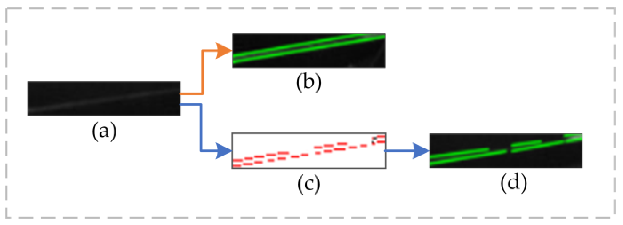
2.1. Overview of ST_LSD

Figure 2 shows the workflow of ST_LSD. Firstly, to protect the edge and remove the noise, the input gray image is preprocessed by adaptive bilateral filtering. Secondly, the improved Otsu algorithm is used to segment the target under complex illumination. The gradient magnitude and gradient direction are calculated, and pixels have a high probability that line segments that pass over are extracted as effective anchors. Thirdly, the anchors are actively grouped into line segments based on the line segment geometry and the alignment of gradient direction. Line segments are verified according to the anchor density and gradient magnitude distribution to control false positives. Finally, according to the line segment aggregation method, the adjacent small line segments that may come from the same line segment are detected and connected.

2.2. Noise Removal Method Combined with Adaptive Bilateral Filtering

Although the camera used in space may adopt a series of measures to suppress stray light and noise, for example, the spectral characteristics of the CCD sensor can be reasonably selected to make it work in the band where the sunlight irradiance is relatively weak and the sensitivity of the CCD sensor is relatively strong. A narrow-band filter is added in front of the lens to filter out some stray light outside the target. However, the impact of complex illumination and spatial noise on image quality still cannot be avoided.

When the original image contains noise, the first step of line segment detection is to filter the image to remove the noise. Line segment detection algorithms generally use linear filtering methods, such as the most commonly used Gaussian filtering. However, linear filtering methods can suppress some edges while removing noise, resulting in edge blurring, which is not conducive to the extraction of subsequent anchors. To address the problem, we adopt a nonlinear filtering method, where a fast adaptive bilateral filter [43] is used instead of the traditional Gaussian filter.

Let $I:{\mathbb{Z}}^2\to ℝ$ represent the input image. The output image $O:{\mathbb{Z}}^2\to ℝ$ after adaptive bilateral filtering is given by:

$$O\left(x\right)=k{(x)}^{-1}{\displaystyle \sum _{y\in \Omega }\eta (y){\varphi }_x\left(I\left(x-y\right)-\theta \left(x\right)\right)I\left(x-y\right)}$$

(1)

the normalized parameter $k\left(x\right)$ is expressed as:

$$k(x)={\displaystyle \sum _{y\in \Omega }\eta (y){\varphi }_x\left(I\left(x-y\right)-\theta \left(x\right)\right)}$$

(2)

where the $\theta \left(x\right)$ is the intensity of the image pixel of interest $I\left(x\right)$, which is set to be $\theta \left(x\right)=I\left(x\right)+f\left(x\right)$. $f\left(x\right)$ is the offset image pixel. $\mathsf{\Omega }$ is a window centered at the origin, and the window in Equations (1) and (2) is usually set to be $\mathsf{\Omega }={\left[-3\rho ,3\rho \right]}^2$. ${\varphi }_x:ℝ\to ℝ$ is the local Gaussian range kernel, which is expressed as:

$${\varphi }_x(i)=\exp \left(-\frac{i^2}{2\sigma {\left(x\right)}^2}\right)$$

(3)

where $\sigma \left(x\right)$ is the standard deviation of the Gaussian function. Importantly, the spatial kernel $\eta :{\mathbb{Z}}^2\to ℝ$ in Equation (1) is a Gaussian kernel, which is calculated as:

$$\eta \left(y\right)=\exp \left(-\frac{{\Vert y\Vert }^2}{2{\rho }^2}\right)$$

(4)

where $\rho$ is also the standard deviation of the Gaussian function.

2.3. Anchor Map Extraction Method Combined with Improved Otsu

To further improve the robustness of the line detection under complex illumination, an adaptive image segmentation method based on the Otsu algorithm is introduced. The traditional two-dimensional Otsu algorithm has limitations in processing images with salt-and-pepper noise and uneven illumination. An improved two-dimensional histogram construction strategy is proposed to improve the extraction of the anchor map.

Suppose $f$ is an image represented in $L$ gray value with $M$ rows and $N$ columns. Let $A$ be the corresponding mean image. The gray level of pixels in $A$ is calculated by:

$$A\left(x,y\right)={\displaystyle \sum _{\tilde{x}=x-(k-1)/2}^{x+(k-1)/2}{\displaystyle \sum _{\tilde{y}=y-(k-1)/2}^{y+(k-1)/2}f(\tilde{x},\tilde{y})}}$$

(5)

where, $A\left(x,y\right)$ and $f\left(x,y\right)$ represent the gray level of the pixel at $\left(x,y\right)$ in $A$ and $f$, respectively. $k$ represents the size of the filter, and the value of $k$ is set to be 3 in our work.

To reduce the complexity, two-dimensional tuples are used to simplify the calculation [44]. Let $f\left(x,y\right)=i$, $A\left(x,y\right)=j$, both of which form the tuple $G\left(x,y\right)$. Then, the tuple contains the gray level of any pixel and its corresponding neighborhood mean gray information. Suppose $n_{ij}$ is the number of occurrences of pixel $\left(x,y\right)$ in the histogram. Thus, the two-dimensional joint probability function $P_{ij}$ is obtained as:

$$P_{ij}=\frac{n_{ij}}{M\times N}$$

(6)

where $x,y\in \left[0,L-1\right]$,$n_{ij}\in \left[0,M\times N\right]$ and ${\displaystyle \sum }_i{\displaystyle \sum }_i{P}_{ij}=1$.

Given a threshold pair $\left(s,t\right)$ consisting of gray threshold $s$ and neighborhood mean gray threshold $t$. The two-dimensional histogram shown in Figure 3 is divided into four areas$A$, $B$, $C$, and$D$ representing the background, edge, target, and noise.

For the space target images, the gray value of the pixel inside the target is roughly the same as the neighborhood mean gray level, and so is the gray value of the spatial background. However, the gray values at the edges of the target and the noise are different. For a given threshold pair $\left(s,t\right)$, image pixels can be divided into two groups, background $T_b$ and objects $T_o$. Their occurrence probabilities can be expressed as:

$${\omega }_b=P\left(T_b\right)={\displaystyle \sum _{i=1}^s{\displaystyle \sum _{j=1}^t{P}_{ij}}}$$

(7)

$${\omega }_o=P\left(T_o\right)={\displaystyle \sum _{i=s}^{L-1}{\displaystyle \sum _{j=t}^{L-1}{P}_{ij}}}$$

(8)

where the mean vectors ${\delta }_b$ and ${\delta }_o$ corresponding to $T_b$ and $T_o$ can be expressed as:

$${\delta }_b={\left({\delta }_{bi},{\delta }_{bj}\right)}^T={\left({\displaystyle \sum _{i=1}^s{\displaystyle \sum _{j=1}^t\frac{i{P}_{ij}}{{\omega }_b},{\displaystyle \sum _{i=1}^s{\displaystyle \sum _{j=1}^t\frac{j{P}_{ij}}{{\omega }_b}}}}}\right)}^T$$

(9)

$${\delta }_O={\left({\delta }_{Oi},{\delta }_{Oj}\right)}^T={\left({\displaystyle \sum _{i=s}^{L-1}{\displaystyle \sum _{j=t}^{L-1}\frac{i{P}_{ij}}{{\omega }_o},{\displaystyle \sum _{i=s}^{L-1}{\displaystyle \sum _{j=t}^{L-1}\frac{j{P}_{ij}}{{\omega }_o}}}}}\right)}^T$$

(10)

Due to the assumption that the occurrence of image data away from the diagonal of the 2D histogram is negligible [45], we can obtain the following approximate expression:

$${\omega }_b+{\omega }_o\approx 1,{\delta }_L={\omega }_b{\delta }_b+{\omega }_o{\delta }_o$$

(11)

The between-class variance of the two-dimensional Otsu algorithm can be defined as follows:

$${\sigma }_B={\displaystyle \sum _{k=0}^1{\omega }_k[({\delta }_k-{\delta }_T){({\delta }_k-{\delta }_T)}^T]}$$

(12)

By using the trace of ${\sigma }_B$ as the measurement of between-class variance, there is:

$$Tr\left({\sigma }_B\right)={\omega }_b\left[{\left({\delta }_{bi}-{\delta }_{Li}\right)}^2+{\left({\delta }_{bj}-{\delta }_{Lj}\right)}^2\right]+{\omega }_o\left[{\left({\delta }_{oi}-{\delta }_{Li}\right)}^2+{\left({\delta }_{oj}-{\delta }_{Lj}\right)}^2\right]$$

(13)

Therefore, the optimal threshold pair $s^{*},t^{*}$ can be obtained by maximizing the between-class variance:

$$\left(s^{\ast },t^{\ast }\right)=\arg \underset{0\le s,t\le L-1}{\max }\left(Tr\left({\sigma }_B\right)\right)$$

(14)

We propose a construction strategy for a two-dimensional histogram. Based on the fact that median filtering can suppress salt-and-pepper noise well, the steps of median filtering are introduced in the construction of a two-dimensional histogram.

Firstly, the original image $f$ is median filtered with $k\times k$ convolution kernel, and median image $M$ can be expressed as:

$$M\left(x,y\right)=med\left\{\begin{array}{r}f(\tilde{x},\tilde{y})|x-\frac{k-1}{2}\le \tilde{x}\le x+\frac{k-1}{2},\\ y-\frac{k-1}{2}\le \tilde{y}\le y+\frac{k-1}{2}\end{array}\right\}$$

(15)

Secondly, according to the obtained median image $M$, the corresponding mean image can be calculated by:

$$A\left(x,y\right)={\displaystyle \sum _{\tilde{x}=x-(k-1)/2}^{x+(k-1)/2}{\displaystyle \sum _{\tilde{y}=y-(k-1)/2}^{y+(k-1)/2}M(\tilde{x},\tilde{y})}}$$

(16)

Finally, we use the median image $M$ and the mean image $A$ to construct a two-dimensional histogram. Based on constructing a two-dimensional gray histogram, the inter-class variance is calculated, and the optimal segmentation threshold is obtained by maximizing the interclass variance. The flow chart is shown in Figure 4. Algorithm 1 shows the implementation process of the improved two-dimensional Otsu algorithm.

Algorithm 1 Improved Otsu method

Input: The gray image f; Initialization parameter. Output: Otsu segmentation result image O.     Step1: median filtering.     Step2: construct the 2D histogram using median image M and median-average     image A.     Step3: calculate the between-class variance Tr.      for i = 0 to 256 do for j = 0 to 256 do            Tr ←$\left({\omega }_b{\left({\delta }_{Li}-{\delta }_{bi}\right)}^2\right)+\left({\omega }_o{\left({\delta }_{Lj}-{\delta }_{oj}\right)}^2\right)/\left({\omega }_b{\omega }_o\right)$     Step4: calculate the optimal threshold for maximizing the between-class variance.            if (Tr > maxvariance) then            maxvariance ←Tr            Trthreshold_s ← i            ithreshold_t ← j            end            end      end      T ← threshold_s      return T     Step5: segment the image by the threshold value T.     ShowImage O.

The improved Otsu method is used to process the image, then the gradient magnitude and gradient orientation are calculated, and the effective anchors are extracted in two steps. Firstly, we use the non-maximum suppression method of the Canny algorithm to extract pixels to obtain general anchors. Secondly, based on the property that the gradient direction of line pixel should be aligned with neighbor pixels. To improve the effectiveness of anchor points and simplify the anchor map, we further verify the general anchors by the orientation and extract general pixels aligned with their neighbor edge pixels as effective anchors. Algorithm 2 presents the implementation process of the anchor map extraction method combined with Otsu.

Algorithm 2 Anchor map extraction method combined with improved Otsu

Input: The image I processed by the improved Otsu method;       the gradient orientation tolerance μ. Output: Effective anchors Ae.       Step1: calculate the gradient magnitude Gm and gradient orientation Go of pixel P(x, y); the center pixel of the neighborhood of pixel P(x, y) is Gp; the interpolation of two gradient amplitudes along the gradient orientation is Gp1 and Gp2, respectively; output the general anchors Ag.           if Gp ≥ Gp1 and Gp ≥ Gp2 then            Ag ← Gp           else            Gp ← 0           end if           return Ag       Step2: verify the general anchors and obtain effective anchors Ae; the gradient orentation of the general anchors Ag is Gg.         if Gg is horizontal then               for pixel P(x, y) in {(x, ya) y−1 ≤ ya ≤ y+1, ya∈N} do                   if angdiff (Gg (x, y), Gg (x, ya)) < μ than                   Ae ← true                   else Ae ← false                   end if               end for         end if         return Ae

2.4. Line Segment Validation and Aggregation

Local strong light may make it impossible to extract effective anchors, which may cause the number of effective anchors to decrease, similar to the partial structure being partially occluded. After anchor map extraction, active grouping, and line segment validation, there may be a situation that the adjacent small line segments from the same line segment fail to connect.

Figure 5 shows this false alarm caused by the change in anchor density. In Figure 5a, there is an obvious line segment. Due to the interference of strong light or noise in the middle of the line segment, the anchor extraction has problems, as shown in Figure 5b, where the number of red anchors in the middle of the line segment (the blue circular region) is less than the threshold of anchor density. After the anchor density method along the line segment, the complete line segment is segmented into two small blue adjacent line segments as shown in Figure 5c. This type of false alarm is likely to occur under complex illumination and noise interference. To solve this problem, an aggregation method for complex illumination is used, which realizes the aggregation of line segments by connecting disjoint line segments that probably came from the same line segment.

Suppose the line segment obtained during the validation phase of the line segment is $l_a$. We call adjacent disjoint segments that probably came from the same line segment as an aggregate candidate line segment $l_b$. The angle difference between the line segments, the distance between endpoints, and the overlap of the line segments are used to judge whether the aggregate candidate line segment $l_b$ can be aggregated. The angle difference between the line segments and the distance between the endpoints are defined as shown in Figure 6.

First, we consider the angle difference between line segments as the first aggregate condition for candidate line segments. Let the angle difference between line segments $l_a$ and $l_b$ be $\theta$. When $\theta$ is less than a certain angle difference threshold ${\tau }_{\theta }$, the two line segments may meet the aggregation requirements and enter the next aggregation conditional validation phase. The angle difference threshold ${\tau }_{\theta }$ is calculated by:

$${\tau }_{\theta }=\left(1-\frac{1}{1+e^{\alpha (\lambda +\beta )}}\right)\gamma$$

(17)

where $\alpha$, $\beta ,$ and $\gamma$ are coefficients and $\lambda$ is a combined normalization coefficient, which can be expressed as:

$$\lambda =\frac{\left|l_b\right|}{\left|l_a\right|}+\frac{d}{{\tau }_d}$$

(18)

where $\left|l_a\right|$ and $\left|l_b\right|$ represent the lengths of the line segments $l_a$ and $l_b$, respectively, and $d$ and ${\tau }_d$ are described below.

Second, we use the endpoint distance between the line segments as the second aggregate condition, as shown in Figure 7. We calculate the Euclidean distance between each endpoint of $l_a$ and $l_b$ and select the smallest endpoint distance as the endpoint distance between $l_a$ and $l_b$. When the two line segments are close enough—in other words, the endpoint distance $d$ meets a certain endpoint distance threshold—it is possible for the two line segments to further aggregate. Set the endpoint distance threshold as ${\tau }_d$, which is proportional to the length of the line segment:

$${\tau }_d=\epsilon \left|\max \left\{\left|l_a\right|,\left|l_b\right|\right\}\right|$$

(19)

where $\epsilon$ is a custom coefficient that satisfies $0<\epsilon <1$.

Finally, we determine whether there is an overlap between the two line segments, as shown in Figure 7. The two segments $l_a$ and $l_b$ are projected onto the $x$-axis, and the overlap length $\psi \left(l_a,l_b\right)$ between $l_a$ and $l_b$ can be obtained. Since the aggregation method is the last part of ST_LSD, it is necessary to prevent false positives while connecting disjoint line segments that may come from the same line segment. Therefore, we set a strict criterion for overlap judgment, where only $\psi \left(l_a,l_b\right)=0$. In other words, the last condition for aggregation can be satisfied only when there is no overlap between the two line segments.

We list five typical relationships between adjacent line segments, as shown in Figure 8. In Figure 8a, the angle difference between line segments $l_{a1}$ and $l_{a2}$ is too large to satisfy the first condition of aggregation. As shown in Figure 8b, although line segments $l_{b1}$ and $l_{b1}$ satisfy the constraint of an angle difference, the endpoint distance between the two line segments is greater than the endpoint distance threshold ${\tau }_d$. This situation does not meet the aggregation condition. In Figure 8c, the angle difference between line segments $l_{c1}$ and $l_{c1}$ is small enough, and the endpoint distance also meets the requirements, but the two line segments overlap and do not meet the aggregation requirements. In Figure 8d, line segments $l_{d1}$ and $l_{d1}$ maintain a collinear disjoint relationship, which is the most ideal situation for aggregation. The two line segments are adjacent and close enough, and all three conditions meet the requirements, so the aggregation operation can be carried out on the two line segments. In Figure 8e, line segments $l_{e1}$ and $l_{e1}$ show a parallel disjoint situation, which is common in structural space targets composed of polyhedrons. In this case, the overlap of the two line segments also makes it impossible to meet the aggregation requirements.

3. Results

We have conducted extensive and detailed experiments, and both quantitative and qualitative experiments are employed for the evaluation of the ST_LSD line segment detection method. The performance of ST_LSD is also compared to LSD, EDLines, Linelet, and AG3line. Among them, LSD and EDLines are the most widely used line segment detectors in recent years, Linelet is a relatively new detector, and the AG3line detector has better effectiveness and faster speed.

3.1. Evaluation Metrics

To scientifically and comprehensively evaluate the performance of ST_LSD, four classical indicators in the field of line segment detection are used in this paper: precision, recall, F-score, and computation time (the unit is milliseconds). Precision, recall, and F-score can be calculated by:

$$Precision=\frac{TP}{TP+FP}$$

(20)

$$Recall=\frac{TP}{TP+FN}$$

(21)

$$F-score=\frac{2PR}{P+R}$$

(22)

where $TP$ is the number of correctly detected line segments called true positive, $FP$ is the false positive and represents the number of incorrectly detected line segments, and $FN$ indicates false negative, that is, the number of line segments that exist in the image but are not detected by the algorithm. In addition, the computation time can reflect the operating efficiency of the algorithm.

In the evaluation of Linelet and AG3line, the valid detection line segment $L_{ed}$ and its ground truth $L_{gt}$ satisfied the following constraints: (1) the angle difference between $L_{ed}$ and $L_{gt}$ is smaller than $\pi /36$; (2) the midpoint of $L_{ed}$ is within one pixel to $L_{gt}$; and (3) the intersection over $L_{gt}$ is larger than the threshold:

$$\frac{L_{ed}\cap L_{gt}}{L_{gt}}\ge {\lambda }_{area}$$

(23)

To avoid setting the overconnection as a true positive, we follow an additional constraint added by AG3line:

$$\frac{L_{ed}\cap L_{gt}}{L_{ed}}\ge {\lambda }_{area}$$

(24)

${\lambda }_{area}$ is the intersection threshold. In this paper, we set it to ${\lambda }_{area}=0.5$ by following the Linelet and AG3line methods.

3.2. Dataset Description

The experimental data in this paper are the optical images of the noncooperative target in space. To collect the optical image data of space targets under different illumination and different noise interference, we built a semiphysical simulation platform to simulate the space environment. The semiphysical simulation platform is shown in Figure 9. The experimental system includes a three-axis turntable, a three degree of freedom guide rail, a camera suitable for the micro-nano satellite platform in space, a real 3U CubeSat, a solar illumination simulator, and the Earth background. In terms of illumination simulation, we use the solar simulator to simulate different illumination intensities and control the movement of the target by rotating the three-axis turntable so as to simulate the situation of different incidence angles of sunlight, and the images of different light intensities and different incidence angles of sunlight are collected by the camera. In addition, the three degrees of freedom guide rail can also control the distance between the target and the tracker. In general, the platform can simulate and collect the pose of the CubeSat in different space environments.

The dataset contains 21 images with a size of $640\times 480$, which simulates 7 images of CubeSat each under high brightness, low brightness, and noise interference. As shown in Figure 10, we list some of the images collected in the micro-nano satellite line segments (MNS-LS) dataset. Figure 10a represents a high-brightness image. We control different illumination intensities on the basis of maintaining high brightness and adjust the distance and angle between the target and the camera to control the local or global high brightness of the target. Figure 10b represents the low-brightness image, and Figure 10c represents the image containing noise. We carefully annotated the dataset with the annotation software and obtained the ground truth line segment of each image in the MNS-LS dataset. In this paper, the performance of ST_LSD is verified by using the MNS-LS dataset.

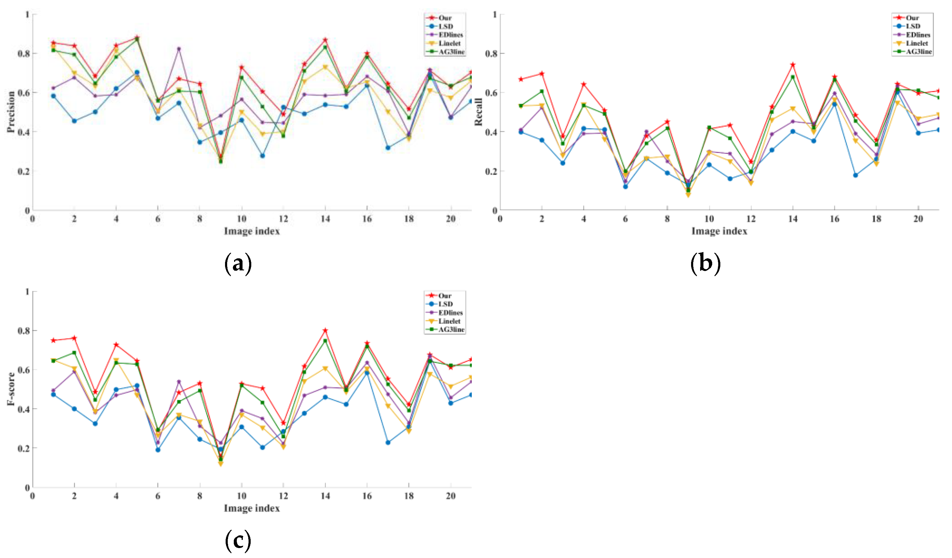
3.3. Quantitative Evaluation Results

Table 1. Performance of different methods on the MNS-LS dataset.

Methods	Precision	Recall	F-Score	Time/ms
LSD	0.4994	0.3123	0.3773	43.76
EDlines	0.5761	0.3700	0.4424	47.23
Linelet	0.5782	0.3696	0.4453	-
AG3line	0.6432	0.4476	0.5222	27.88
ST_LSD	0.6807	0.4847	0.5598	33.37

provides the line segment detection results of the five methods on the MNS-LS dataset. As shown in the results, ST_LSD is better than other methods in precision, recall, and F-score. This is mainly attributed to the adaptive bilateral filtering and anchor map extraction method combined with Otsu introduced in this paper. In addition, the aggregation method introduced also ensures the integrity of line segments as much as possible. AG3line ranks second in precision, recall, and F-score because AG3line uses the combination of active grouping and geometric gradients to facilitate the extraction of line segments, thus ensuring the recall of line segments. In precision, AG3line adopts two methods to control false positives from coarse to fine, which is also more effective. EDlines and Linelet perform very similarly in three aspects, but Linelet does better overall in precision and F-score. The performance of Linelet in precision benefits from its effective control of false positives in the validation phase. After the original author’s optimization, the performance of EDlines is significantly improved, and it performs better than Linelet in the recall, but its precision and F-score are worse than Linelet, which indicates that EDlines detect more ground truths as well as more false positives than Linelet. The classical LSD performs poorly and has a certain gap with the previous four detectors.

Figure 11 shows the detailed performance of the different methods in precision, recall, and F-score on the MNS-LS dataset. As shown in the picture, ST_LSD performs better on images 1–6 with high-brightness illumination. For images with a large gradient difference between the background and the target, the anchor map extraction method combined with Otsu can effectively separate the background and target so as to extract more meaningful line segments. For images 7–13 with too-dark illumination, the gradient difference between the background and the target is very small. The anchor map extraction method combined with Otsu fails to effectively separate the target and the background, which leads to the performance degradation of ST_LSD in images 7–13. However, compared with other traditional methods, ST_LSD still maintains certain advantages. In addition, for images 14–21 with noise interference, ST_LSD is slightly better in all aspects, mainly due to the bilateral filtering method introduced in this paper, which can remove noise and effectively maintain edge information. In general, compared with other methods, ST_LSD performs better with complex illumination and noise interference.

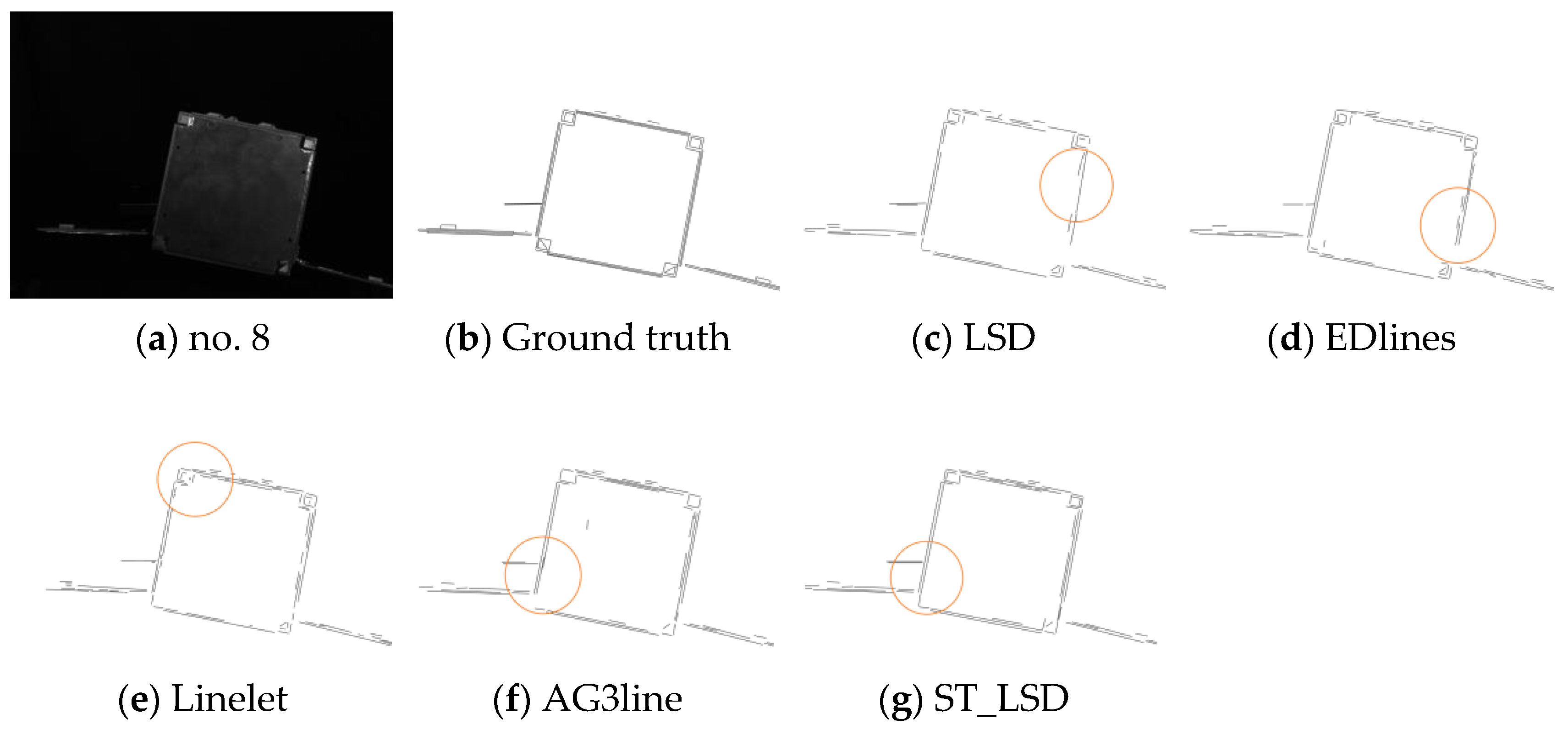
3.4. Qualitative Comparison

Figure 12, Figure 13 and Figure 14 show the line segment detection results on images no. 3, 8, and 21 of the MNS-LS dataset, respectively. The image in Figure 12a is a challenging situation, where high-brightness illumination poses a challenge to the detection of the quadrangular structure on the front and makes the detected line segment incomplete. As shown in Figure 12c,d, LSD and EDlines can detect part of the quadrangular structure, but the number of line segments detected by LSD on the solar panel is too small, and it is not robust to the situation of complex illumination, while EDlines causes many complete line segments to break. The orange circular region in Figure 12e shows that Linelet produces many fractures and more false positives than ST_LSD. We can see from the orange circular region in Figure 12f that AG3line does not perform well in the detection of the quadrille structure on the front and some line segments are fractured. In comparison, as shown in the orange circular region in Figure 12g, ST_LSD can effectively extract some obvious quadrangular structure line segments with high-brightness illumination, and it can maintain the integrity of line segments, such as detecting solar panel line segments while rejecting some false positives.

Figure 13a shows the situation with low-brightness illumination. LSD still has the problem of detecting too few line segments and failing to detect the line segments on the right side of the square surface. EDlines also has the same problem, but the optimized EDlines performs better than LSD. As shown in the orange circular region in Figure 13e, Linelet detects the most fracture line segments and produces the most fractures. AG3line performs better than the others except for ST_LSD. ST_LSD detects more complete line segments and also rejects some false positives on the square.

Figure 14a represents the situation with noise interference. As shown in Figure 14, ST_LSD outperforms the others in rejecting false positives. In addition, ST_LSD detects the largest number of meaningful line segments. Many false positives are generated by LSD, EDlines, and Linelet. LSD and EDlines split a complete line segment into many small lines, while Linelet is found to produce many fractures and more false positives than ST_LSD.

The quantitative evaluation in

Table 2. Quantitative evaluation of the performance on images no. 3, 8, and 21 of the dataset.

Algorithm Image	LSD				EDlines				Linelet				AG3line				ST_LSD
	#3	#8	#21	Mean	#3	#8	#21	Mean	#3	#8	#21	Mean	#3	#8	#21	Mean	#3	#8	#21	Mean
Precision	0.5	0.35	0.56	0.47	0.58	0.42	0.63	0.54	0.63	0.43	0.66	0.57	0.64	0.6	0.68	0.64	0.68	0.64	0.7	0.67
Recall	0.24	0.19	0.41	0.28	0.28	0.25	0.47	0.33	0.28	0.27	0.49	0.35	0.34	0.42	0.57	0.44	0.38	0.45	0.61	0.48
F-score	0.32	0.25	0.47	0.25	0.38	0.31	0.54	0.41	0.39	0.34	0.56	0.43	0.44	0.49	0.62	0.52	0.49	0.53	0.65	0.56
Time(ms)	36.8	35.1	51.8	41.2	41.6	38.6	58.3	46.2	-	-	-	-	25.2	23.4	35.3	28.0	29.1	28.3	42.4	33.3

corresponds to the qualitative results. It can be seen that ST_LSD has good performance in the detection performance of three images. ST_LSD achieves the top score in precision, recall, and F-score. Note that the computational time of ST_LSD ranks second, which is only slightly slower than AG3line.

4. Discussion

This section describes the parameter settings and algorithmic complexity of ST_LSD. In addition, future research directions are also proposed.

4.1. Parameter Settings

To ensure the effectiveness of the algorithm comparison, we discuss the parameter settings of the four comparison methods of LSD, EDLines, Linelet, and AG3line. Finally, we use the source code and default parameters provided by the original author of the algorithm. We list some important parameters of the four methods. LSD sets the minimum gradient magnitude to 5.2; EDLines uses a $5\times 5$ Gaussian kernel filter with $\sigma =1$ to filter the image; Linelet sets the linelet length difference threshold ${\tau }_{len}$ to 3; the jump distance of anchor points in AG3lines is set to 10, and the gradient orientation threshold is $\pi /8$. Except for EDLines, the implementations of the other three methods are available on the websites provided by the relevant authors. Since the original EDLines code is no longer available on the website provided by the author, we used the optimized code of the original authors to improve the performance of EDLines and enhance the comparability of EDLines. Their implementations are available on the authors’ websites [46,47,48,49]. Our algorithm determines the internal parameters during the experiment. The parameters of ST_LSD are as follows:

1.

Suppressing image noise: in Section 2.2, the image is filtered by using an adaptive bilateral filter with a $3\times 3$ filter window.

2.

Gradient orientation tolerance: in Section 2.3, following the LSD [21] method, two pixels’ gradient orientations are aligned when the difference between their angles is smaller than $\pi /8$.

3.

Angle difference threshold: in Section 2.4, following the LSM [29] method, the coefficients in the angle difference threshold are set as $\alpha =-2$, $\beta =-1.5$, and $\gamma ={22.5}^{°}$.

4.

Endpoint distance threshold: in Section 2.4, $\epsilon =0.09$, and the algorithm has the best effect in the experiment.

4.2. The Complexity of ST_LSD

For the ST_LSD algorithm, the computational cost mainly includes image preprocessing, anchor map extraction, active grouping, line segment validation, and line segment aggregation. We discuss the complexity by testing the computation time of the four algorithms.

The computation times of LSD, EDlines, AG3line, and ST_LSD are compared using the MNS-LS dataset. Linelet is only available for the MATLAB vision, while ST_LSD and the other three algorithms are implemented by Visual C ++ Compiler. It is unfair to use the C ++ version of ST_LSD to compare with Linelet. Therefore, in the comparison of computation time, ST_LSD only considers LSD, EDlines, and AG3line running on the same hardware environment and the same compiler. The tests were performed on the same laptop with a Win10 system (Intel Core i7-8750H, 2.20 GHz CPU, and 16 GB RAM). To further reduce the error, we employed 30 tests for each image and took the average computation time as the final result.

Figure 15 shows the computation times of the four methods on the MNS-LS dataset, where it can be seen that all of them processed each image within about 80 milliseconds (ms). AG3line is the fastest, and the computation time is stable within 20–30 ms because its active grouping method reduces the computation time. ST_LSD ranks second, and its time distribution is also relatively stable. There are two reasons why ST_LSD is slower than AG3line. First, ST_LSD introduces bilateral filtering to replace the original Gaussian filtering processing method. Bilateral filtering can keep image edge information well, but it also takes more time than Gaussian filtering. Second, the anchor map extraction method combined with Otsu adopted by ST_LSD also requires a certain computation time. But in general, ST_LSD achieves good performance in computation time, which is faster than the classical linear-time detector LSD and the optimized EDlines. The difference between the computation time of optimized EDlines and LSD is not very large, but their time distributions are not as stable as ST_LSD. The optimized EDlines has a significant improvement in the detection effect, which overtakes the traditional LSD, but it does not maintain the advantage of fast and real-time computing time, and, on the other hand, it is a little slower than LSD.

Our experimental results demonstrate that ST_LSD can perform well under complex illumination conditions and noise interference. The introduced bilateral filtering method can maintain the edge information of the image well, the anchor map extraction method combined with Otsu can be applied to complex illumination, and the aggregation method also has a certain effect on ensuring the integrity of line segments. Compared with traditional line segment detection methods, ST_LSD achieves a good balance in extracting complete line segments and controlling false positives. Moreover, it performs well in computation time. Of course, the traditional line detection method cannot avoid false alarms, and ST_LSD also produces certain false alarms in complex space environments. The causes of false alarms are mainly the following three: (1) the dramatic change in illumination affects the extraction of anchor points, resulting in too few anchor points; (2) a change in anchor density in the line segment validation phase; and (3) some fixed threshold parameters in the line segment aggregation phase. In general, ST_LSD has a good improvement in detection precision and visual effects.

In addition, it cannot be ignored that other traditional detectors have their own advantages: (1) LSD does not need parameter adjustment and can control certain false positives; (2) EDlines has a fast computation time and can run in real time. Although the computation time of optimized EDlines has increased, the detection effect has been significantly improved; (3) Linelet can extract more local line segments, although it produces more fracture line segments; and (4) AG3line can effectively control false negatives and false positives while maintaining a fast running speed.

5. Conclusions

On the whole, we aimed to address the problem that traditional line segment detection methods easily fail in the presence of complex illumination and noise interference. To further improve the performance of space target segment detection, we propose a robust line segment detector for space applications called ST_LSD in this paper. The proposed detector can effectively solve the phenomenon of line segment fracture caused by complex illumination and noise interference. The image data are collected through a semiphysical simulation platform, and the MNS-LS dataset is constructed precisely to verify the performance of ST_LSD. Our quantitative and qualitative evaluation results show that ST_LSD is superior to traditional detectors in terms of detection accuracy and visual effect under complex illumination and noise interference.

There are still some limitations to the proposed approach. It can be seen from the experimental results that the speed of ST_LSD needs to be further improved. In future studies, we suggest three extensions to the work presented in this paper: (1) optimize the active grouping and line segment verification of ST_LSD to be more suitable for real-time application scenarios; (2) expand and optimize the existing MNS-LS dataset to meet more mission requirements; and (3) extend ST_LSD’s algorithm to detect the circles, which occur frequently in space targets, to adapt to more and more extensive space on-orbit service missions.

References

1. Cassinis, L.P.; Fonod, R.; Gill, E.; Ahrns, I.; Fernandez, J.G. CNN-Based Pose Estimation System for Close-Proximity Operations Around Uncooperative Spacecraft. In Proceedings of the AIAA Scitech 2020 Forum, Orlando, FL, USA, 6–10 January 2020; pp. 1–16. [Google Scholar]
2. Chen, B.; Cao, J.W.; Parra, A.; Chin, T.J. Satellite pose estimation with deep landmark regression and nonlinear pose refinement. In Proceedings of the 2019 IEEE/CVF International Conference on Computer Vision Workshop, Seoul, Korea, 27–28 October 2019; pp. 2816–2824. [Google Scholar]
3. Huo, Y.; Li, Z.; Zhang, F. Fast and accurate spacecraft pose estimation from single shot space imagery using box reliability and keypoints existence judgments. IEEE Access 2020, 8, 216283–216297. [Google Scholar] [CrossRef]
4. Kendall, A.; Grimes, M.; Cipolla, R. Posenet: A convolutional network for real-time 6-dof camera relocalization. In Proceedings of the 2015 IEEE International Conference on Computer Vision, Santiago, Chile, 7–13 December 2015; pp. 2938–2946. [Google Scholar]
5. Sharma, S.; D’Amico, S. Neural network-based pose estimation for noncooperative spacecraft rendezvous. IEEE Trans. Aerosp. Electron. Syst. 2020, 56, 4638–4658. [Google Scholar] [CrossRef]
6. Proença, P.F.; Gao, Y. Deep Learning for Spacecraft Pose Estimation from Photorealistic Rendering. In Proceedings of the 2020 IEEE International Conference on Robotics and Automation (ICRA), Paris, France, 31 May–31 August 2020; pp. 6007–6013. [Google Scholar]
7. Gupta, K.; Petersson, L.; Hartley, R. Cullnet: Calibrated and pose aware confidence scores for object pose estimation. In Proceedings of the 2019 IEEE/CVF International Conference on Computer Vision Workshop, Seoul, Korea, 27–28 October 2019; pp. 2758–2766. [Google Scholar]
8. Song, J.; Rondao, D.; Aouf, N. Deep learning-based spacecraft relative navigation methods: A survey. Acta Astronaut. 2022, 191, 22–40. [Google Scholar] [CrossRef]
9. Yu, P.; Wang, C.; Wang, Z.; Yu, J.; Kneip, L. Accurate line-based relative pose estimation with camera matrices. IEEE Access 2020, 8, 88294–88307. [Google Scholar] [CrossRef]
10. Lin, B.; Zhong, L.; Sheng, Z.; Yang, X.; Yang, Y.; Wang, K.; Zhang, X. A New Pattern for Detection of Streak-Like Space Target from Single Optical Images. IEEE Trans. Geosci. Remote Sens. 2022, 60, 1–13. [Google Scholar] [CrossRef]
11. Wang, D.; Liu, Q.; Yin, Q.; Ma, F. Fast Line Segment Detection and Large Scene Airport Detection for PolSAR. Remote Sens. 2022, 14, 5842. [Google Scholar] [CrossRef]
12. Liu, N.; Cui, Z.; Cao, Z.; Pi, Y.; Dang, S. Airport detection in large-scale SAR images via line segment grouping and saliency analysis. IEEE Geosci. Remote Sens. Lett. 2018, 15, 434–438. [Google Scholar] [CrossRef]
13. Tang, G.; Xiao, Z.; Liu, Q.; Liu, H. A novel airport detection method via line segment classification and texture classification. IEEE Geosci. Remote Sens. Lett. 2015, 12, 2408–2412. [Google Scholar] [CrossRef]
14. Jia, X.; Huang, X.; Zhang, F.; Gao, Y.; Yang, C. Robust Line Matching for Image Sequences Based on Point Correspondences and Line Mapping. IEEE Access 2019, 7, 39879–39896. [Google Scholar] [CrossRef]
15. Chia, A.Y.; Rajan, D.; Leung, M.K.; Rahardja, S. Object recognition by discriminative combinations of line segments, ellipses, and appearance features. IEEE Trans. Pattern Anal. Mach. Intell. 2012, 34, 1758–1772. [Google Scholar] [CrossRef]
16. Luo, Y.T.; Zhao, L.Y.; Zhang, B.; Jia, W.; Xue, F.; Lu, J.T.; Zhu, Y.H.; Xu, B.Q. Local line directional pattern for palmprint recognition. Pattern Recognit. 2016, 50, 26–44. [Google Scholar] [CrossRef]
17. Hofer, M.; Maurer, M.; Bischof, H. Efficient 3D scene abstraction using line segments. Comput. Vis. Image Understand 2017, 157, 167–178. [Google Scholar] [CrossRef]
18. Zhong, L.; Qin, J.; Yang, X.; Zhang, X.; Shang, Y.; Zhang, H.; Yu, Q. An Accurate Linear Method for 3D Line Reconstruction for Binocular or Multiple View Stereo Vision. Sensors 2021, 21, 658. [Google Scholar] [CrossRef] [PubMed]
19. Ballard, D.H. Generalizing the Hough transform to detect arbitrary shapes. Pattern Recognit. 1981, 13, 111–122. [Google Scholar] [CrossRef] [Green Version]
20. Kiryati, N.; Eldar, Y.; Bruckstein, A.M. A probabilistic Hough transform. Pattern Recognit. 1991, 24, 303–316. [Google Scholar] [CrossRef]
21. Galamhos, C.; Matas, J.; Kittler, J. Progressive probabilistic Hough transform for line detection. CVPR 1999, 1, 554–560. [Google Scholar]
22. Xu, L.; Oja, E.; Kultanen, P. A new curve detection method: Randomized Hough transform (RHT). Pattern Recognit. Lett. 1990, 11, 331–338. [Google Scholar] [CrossRef]
23. Fernandes, L.A.F.; Oliveira, M.M. Real-time line detection through an improved Hough transform voting scheme. Pattern Recognit. 2008, 41, 299–314. [Google Scholar] [CrossRef]
24. Du, S.; Tu, C.; Van Wyk, B.J.; Chen, Z. Collinear segment detection using HT neighborhoods. IEEE Trans. Image Process. 2011, 20, 3612–3620. [Google Scholar]
25. Almazan, E.J.; Tal, R.; Qian, Y.; Elder, J.H. MCMLSD: A dynamic programming approach to line segment detection. In Proceedings of the 2017 IEEE Conference on Computer Vision and Pattern Recognition, Honolulu, HI, USA, 21–26 July 2017; Volume 10, pp. 5854–5862. [Google Scholar]
26. Burns, J.B.; Hanson, A.R.; Riseman, E.M. Extracting straight lines. IEEE Trans. Pattern Anal. Mach. Intell. 1986, 8, 425–455. [Google Scholar] [CrossRef]
27. Desolneux, A.; Moisan, L.; Morel, J.M. Meaningful alignments. Int. J. Comput. Vis. 2000, 40, 7–23. [Google Scholar] [CrossRef]
28. Lu, X.; Yao, J.; Li, L.; Liu, Y.; Zhang, W. Edge chain detection by applying Helmholtz principle on gradient magnitude map. In Proceedings of the 2016 23rd International Conference on Pattern Recognition, Cancun Center, Cancun, Mexico, 4–8 December 2016; pp. 1364–1369. [Google Scholar]
29. Gioi, R.G.V.; Jakubowicz, J.; Morel, J.M.; Randall, G. LSD: A fast line segment detector with a false detection control. IEEE Trans. Pattern Anal. Mach. Intell. 2021, 32, 722–732. [Google Scholar] [CrossRef]
30. Akinlar, C.; Topal, C. EDLines: A real-time line segment detector with a false detection control. Pattern Recognit. Lett. 2011, 32, 1633–1642. [Google Scholar] [CrossRef]
31. Topal, C.; Akinlar, C. Edge Drawing: A combined real-time edge and segment detector. J. Visual Commun. Image Represent. 2012, 23, 862–872. [Google Scholar] [CrossRef]
32. Akinlar, C.; Topal, C. EDPF: A real-time parameter-free edge segment detector with a false detection control. Int. J. Pattern Recogn. 2012, 26, 1–22. [Google Scholar] [CrossRef]
33. Wang, Y.; Yu, L.; Xie, H.; Lei, T.; Guo, Z.; Qi, M. Line detection algorithm based on adaptive gradient threshold and weighted mean shift. Multimed. Tools. Appl. 2016, 75, 16665–16682. [Google Scholar] [CrossRef]
34. Lu, X.; Yao, J.; Li, K.; Li, L. CannyLines: A parameter-free line segment detector. In Proceedings of the 2015 IEEE International Conference on Image Processing, Quebec City, QC, Canada, 27–30 September 2015; pp. 507–511. [Google Scholar]
35. Salaun, Y.; Marlet, R.; Monasse, P. Multiscale line segment detector for robust and accurate SfM. In Proceedings of the IEEE 2016 23rd International Conference on Pattern Recognition, Cancun Center, Cancun, Mexico, 4–8 December 2016; pp. 2000–2005. [Google Scholar]
36. Yu, Q.; Xu, G.; Cheng, Y.; Zhu, Z. PLSD: A Perceptually Accurate Line Segment Detection Approach. IEEE Access 2020, 8, 42595–42607. [Google Scholar] [CrossRef]
37. Hamid, N.; Khan, N. LSM: Perceptually accurate line segment merging. J. Electron Imaging. 2016, 25, 1–12. [Google Scholar] [CrossRef]
38. Cho, N.G.; Yuille, A.; Lee, S.W. A novel linelet-based representation for line segment detection. IEEE Trans. Pattern Anal. Mach. Intell. 2018, 40, 1195–1208. [Google Scholar] [CrossRef]
39. Liu, Y.; Xie, Z.; Liu, H. LB-LSD: A length-based line segment detector for real-time applications. Pattern Recognit. Lett. 2019, 128, 247–254. [Google Scholar] [CrossRef]
40. Liu, Y.; Xie, Z.; Liu, H. An Adaptive and Robust Edge Detection Method Based on Edge Proportion Statistics. IEEE Trans. Image Process. 2020, 29, 5206–5215. [Google Scholar] [CrossRef] [PubMed]
41. Zhang, Y.; Wei, D.; Li, Y. AG3line: Active Grouping and Geometry-Gradient Combined Validation for Fast Line Segment Extraction. Pattern Recognit. 2021, 113, 1–11. [Google Scholar] [CrossRef]
42. Proietti, A.; Panella, M.; Leccese, F.; Svezia, E. Dust detection and analysis in museum environment based on pattern recognition. Measurement 2015, 66, 62–72. [Google Scholar] [CrossRef]
43. Gavaskar, R.G.; Chaudhury, K.N. Fast Adaptive Bilateral Filtering. IEEE Trans. Image Process. 2019, 28, 779–790. [Google Scholar] [CrossRef] [Green Version]
44. Chen, Q.; Zhao, L.; Kuang, G.; Wang, N.; Jiang, Y. Modified two-dimensional Otsu image segmentation algorithm and fast realization. IET Image Process. 2012, 6, 426–433. [Google Scholar] [CrossRef]
45. Huang, L.; Fang, Y.; Zuo, X.; Yu, X. Automatic Change Detection Method of Multitemporal Remote Sensing Images Based on 2D-Otsu Algorithm Improved by Firefly Algorithm. J. Sensors. 2015, 3, 1–8. [Google Scholar] [CrossRef] [Green Version]
46. LSD Web Site. Available online: http://www.ipol.im/pub/art/2012/gjmr-lsd (accessed on 5 March 2022).
47. EDLines Web Site. Available online: http://ceng.anadolu.edu.tr/cv/EDLines (accessed on 6 March 2022).
48. Linelet Web Site. Available online: https://github.com/NamgyuCho (accessed on 14 March 2022).
49. AG3line Web Site. Available online: https://github.com/weidong-whu/AG3line (accessed on 3 April 2022).
Figure 1. The line segment fracture phenomenon is caused by the reduced number of anchors. (a) The original image. (b) Theoretical output image. (c) Anchor map after AG3line processing. (d) Actual output image.
Aerospace 10 00195 g001
Figure 2. The workflow of ST_LSD.
Aerospace 10 00195 g002
Figure 3. Planar projection of two-dimensional gray histogram.
Aerospace 10 00195 g003
Figure 4. Flow chart of the algorithm.
Aerospace 10 00195 g004
Figure 5. False alarm caused by anchor density change. (a) The original image. (b) Errors in anchor map extraction. (c) The complete line segment is divided into two small line segments.
Aerospace 10 00195 g005
Figure 6. Schematic diagram of the angle difference between segments and the distance between endpoints.
Aerospace 10 00195 g006
Figure 7. Schematic diagram of the overlap length between two line segments.
Aerospace 10 00195 g007
Figure 8. Typical adjacent line segment relationship. (a) The angle difference is too large. (b) The endpoint distance between line segments exceeds the threshold value. (c) The line segments overlap. (d) The ideal situation of collinear disjoint. (e) The parallel disjoint but overlapping situation.
Aerospace 10 00195 g008
Figure 9. Semiphysical simulation platform.
Aerospace 10 00195 g009
Figure 10. Some images in the MNS-LS dataset. (a) High-brightness image. (b) Low-brightness image. (c) An image with noise.
Aerospace 10 00195 g010
Figure 11. Detailed performance of different methods on the MNS-LS dataset. (a) Precision. (b) Recall. (c) F-score.
Aerospace 10 00195 g011
Figure 12. Line segment detection result on image no. 3 of the dataset.
Aerospace 10 00195 g012
Figure 13. Line segment detection result on image no. 8 of the dataset.
Aerospace 10 00195 g013
Figure 14. Line segment detection result on image no. 21 of the dataset.
Aerospace 10 00195 g014
Figure 15. The computation times of different methods on dataset images.
Aerospace 10 00195 g015