Article

Integrated Guidance-and-Control Design for Three-Dimensional Interception Based on Deep-Reinforcement Learning

Key Laboratory of Transient Physics, Nanjing University of Science and Technology, Nanjing 210094, China
*
Author to whom correspondence should be addressed.
Aerospace 2023, 10(2), 167; https://doi.org/10.3390/aerospace10020167
Submission received: 15 January 2023 / Revised: 5 February 2023 / Accepted: 9 February 2023 / Published: 11 February 2023

Abstract

:
This study applies deep-reinforcement-learning algorithms to integrated guidance and control for three-dimensional, high-maneuverability missile-target interception. Dynamic environment, reward functions concerning multi-factors, agents based on the deep-deterministic-policy-gradient algorithm, and action signals with pitch and yaw fins as control commands were constructed in the research, which control the missile in order to intercept targets. Firstly, the missile-interception system includes dynamics such as the inertia of the missile, the aerodynamic parameters, and fin delays. Secondly, to improve the convergence speed and guidance accuracy, a convergence factor for the angular velocity of the target line of sight and deep dual-filter methods were introduced into the design of the reward function. The method proposed in this paper was then compared with traditional proportional navigation. Next, many simulations were carried out on high-maneuverability targets with different initial conditions by randomization. The numerical-simulation results showed that the proposed guidance strategy has higher guidance accuracy and stronger robustness and generalization capability against the aerodynamic parameters.

1. Introduction

The method traditionally used for missile guidance is the dual-loop control of the guidance and control loops based on the assumption of spectral separation. Although this method has been widely used, the application scenarios are mainly limited to low-speed or fixed targets. This method can significantly degrade the guidance-control system’s performance or even cause missile instability for high-speed and large maneuvering targets. This is because the dual-loop design method ignores the coupling relationship with the system at the beginning of the design. Moreover, even if the control method compensates for this, it cannot fundamentally resolve the model defects caused by ignoring the coupling relationship. The integrated guidance and control (IGC) design method utilizes the coupling relationship between guidance and control loops. The IGC was first proposed by Williams [1]. It generates fin-deflection-angle commands based on the missile’s relative motion information and the missile body’s attitude information to achieve missile interception of targets and ensure stability within the missile dynamics. Based on the control signal provided by the guidance law, the missile can adjust its flight state. Some commonly used methods include the parallel approach, proportional guidance (PN), augmented proportional guidance (APN), and zero-control miss-distance quantity. Proportional guidance has been widely used because of its simple structure and easy implementation [2,3]. When attacking fixed targets or intercepting small maneuvering targets, PN has shown significant interception performance. In recent years, with the rapid development of missile-based assault and defense technology, target maneuverability has also been significantly improved. One study [4] introduced a new algorithm for split event detection and target tracking using the joint integrated probabilistic data association (JIPDA) algorithm. The results showed a significant improvement in the actual track rate and root-means-square-error performance. Consequently, PN cannot cope with high-speed, highly maneuverable targets.
Moreover, the interception efficiency of PN has significantly reduced. Augmented proportional navigation (APN) [5] compensates for target maneuverability to some extent by superimposing target-acceleration information on the PN guidance command. Notably, the prerequisite for APN implementation is anticipating the target’s acceleration information. However, this process is challenging for practical applications. Thus far, with the continuous development of the nonlinear control theory, several nonlinear control methods have been used to design guidance laws.
Moreover, unique tactical requirements, such as angle-of-attack constraints and energy control, have been met based on ensuring guidance accuracy. Commonly used design methods include sliding-mode control [6], adaptive control [7], inverse control [8], model predictive control [9], and active-disturbance-rejection control [10]. An analysis of the existing literature on the governing laws of nonlinear methods shows that sliding-mode-control methods are highly robust. However, nonmatching uncertainty estimation and jitter problems are essential factors limiting their further development. Adaptive control can combine multiple control methods. However, it significantly reduces the control effect when unmodeled dynamics occur in the system. The inverse method is suitable for systems with a strict feedback form, and the guidance performance depends on the system’s modeling accuracy. Active-disturbance-rejection control has a significant anti-disturbance capability for time-varying, nonlinear, and unmodeled state disturbances [11]. However, several parameters need to be adjusted, the tuning process is highly subjective, and the stability-theory study of the active-disturbance-rejection-control method still needs to be effectively verified. Owing to aerodynamic-parameter uptake, external disturbances, target maneuvers, and other factors, an IGC system might have several matching or nonmatching uncertainties, which pose a significant challenge to the accurate modeling of the system. Moreover, the performances of existing optimal control algorithms mostly depend on the modeling accuracy. Therefore, this study investigates a three-dimensional (3D) IGC algorithm based on deep-reinforcement learning with a model-free reinforcement-learning theory to address this challenge.
With the continuous development of computer technology, a new generation of artificial intelligence (AI) technology, represented by machine learning, has made significant progress in many fields of application [12]. In the application field of guidance control, AI technologies have significant potential advantages over traditional technologies in terms of accuracy, efficiency, real-time, and predictability [13]. As an essential branch of machine learning, reinforcement learning (RL) is a third type of machine learning, distinct from supervised and unsupervised learning. Along with the continuous technical innovation of deep learning (DL), DRL algorithms that combine DL and RL in depth have gradually emerged and have been widely investigated. Currently, DRL techniques are commonly used in the intelligent planning of spacecraft-transfer trajectories, spacecraft entry, descent-and-landing-trajectory guidance, and rover-trajectory guidance, showing good performance and broad application prospects. For example, in [14], RL was applied to the problem of autonomous planetary landing for the first time. An adaptive-guidance algorithm was designed without offline trajectory generation or real-time tracking to achieve a robust, fuel-efficient, and accurate landing. In [15], a six-degree-of-freedom planetary-power descent-and-landing method based on DRL was developed to verify the feasibility of a Mars landing. The use of such algorithms in the design of interception-guidance laws has also attracted considerable attention. Although several related studies have been conducted, they are still in the initial stages. Brian Gaudet [16] used reinforcement meta-learning to design a discrete action space for intercept-guidance laws for maneuvering targets outside the atmosphere. This method directly maps the guide head’s line-of-sight angle and its rate of change to the commanded thrust of the missile thruster, approximating the end-to-end control effect. This study is an initial attempt to apply DRL algorithms to design guidance laws. It provides a new approach to the creation of DRL-based guidance laws. However, this discrete action does not apply to ballistic interception in continuous-action space in the atmosphere. Thus far, studies on missile-interception-guidance laws in two-dimensional spaces have been conducted gradually. In [17], a homing-guidance-law model based on deep Q-Network (DQN) with prioritized experience replay is proposed for the interception of high-speed maneuvering targets. The authors of [18,19] applied a deep-deterministic-policy gradient (DDPG) algorithm to an interceptor-guidance-law design in a two-dimensional space to demonstrate that the training agent can effectively improve the learning efficiency and interception effect of the agent. In [20], a variable-coefficient-proportional-guidance law based on RL is proposed based on the traditional PN law using a Q-learning method, which is still a PN law and not entirely based on RL, to design the guidance law. The authors of [21] investigated the classical terminal-angle-constraint-guidance law using RL and applied it to the relative motion-guidance problem for near-linear orbits. The aforementioned mathematical models are primarily based on two-dimensional spatial states, which may simplify the design of the guidance law. They have not fully demonstrated the advantages of the DRL algorithm in the 3D-guidance-law design. Moreover, other studies [22,23,24,25,26] consider constraints ion guidance and control.
This study proposes a DRL algorithm for the IGC problem of interception with high-speed, highly maneuverable targets. The design considers the continuity of the missile’s action space. In addition, training and validation of the results were performed in a 3D space. The contributions of this study beyond those of previous studies are as follows:
(1)
Multiple constraints were satisfied in the guidance field to attack the target accurately, and the effectiveness and feasibility are verified by the random initialization of the missile and target states.
(2)
The convergence speed and guidance accuracy were effectively improved by introducing the convergence factor of the angular velocity of the target line-of-sight.
(3)
The deep dual filter (DDF) method was introduced when designing the DRL algorithm, guaranteeing better performance under the same training burden.
The rest of this paper is organized as follows. The 3D engagement dynamics and equations for the IGC are introduced in Section 2. The DRL algorithms are presented in Section 3, and the modeling of the IGC problem based on the DRL is presented in Section 4. Numerical simulations were conducted, and the results are shown in Section 5. Section 6 provides the conclusions.

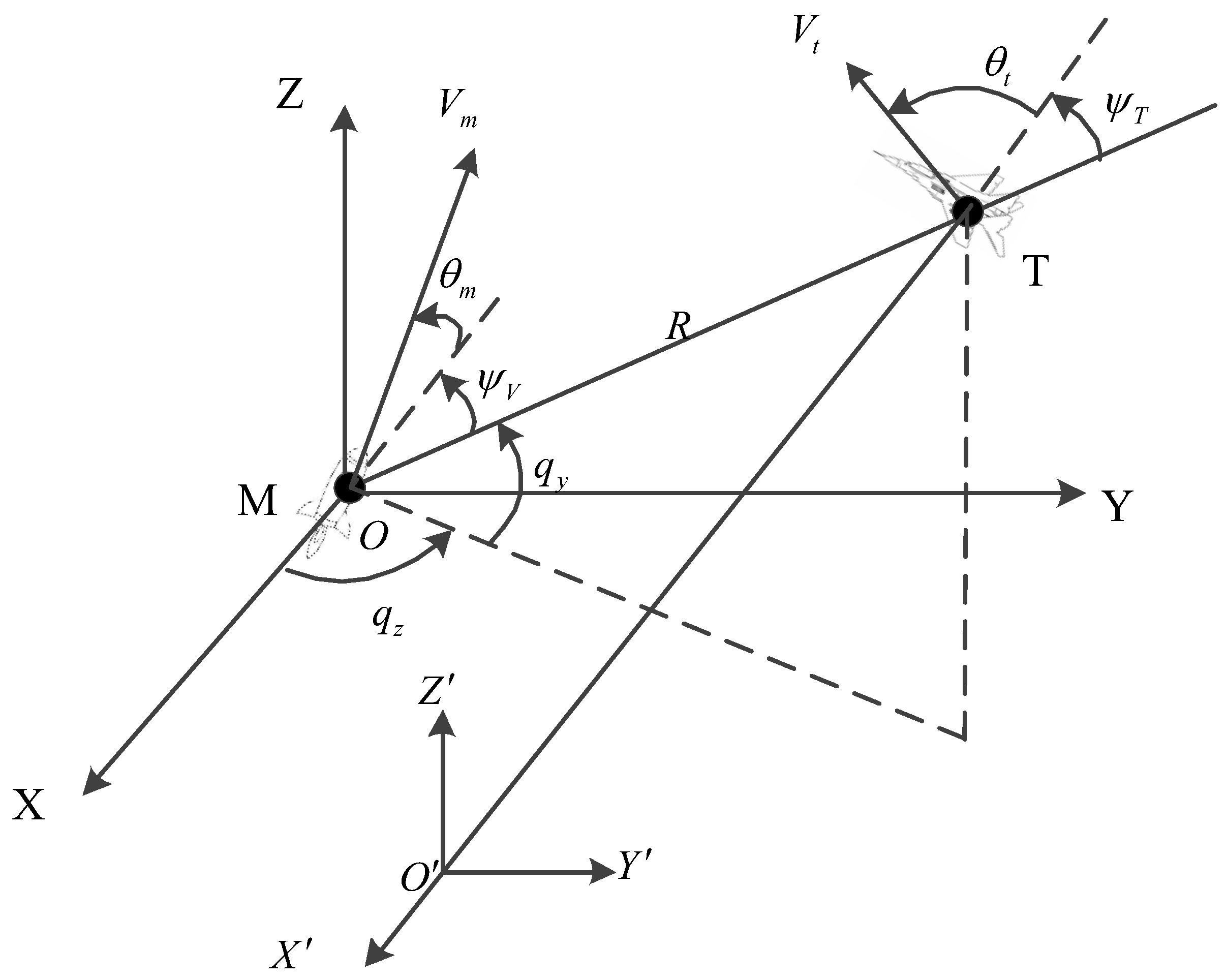
2. Three-Dimensional IGC Model

Missile equations of motion describe the relationship between motion parameters acting on a missile, generally consisting of kinetic and kinematic equations. The following basic assumptions are made.
Assumption ①: No engine work is considered. Since P = 0, with P as the engine thrust, which can be seen as the state in which the engine work finishes, the missile’s mass is unchanged.
Assumption ②: The missile structure is axisymmetric ( J y = J z ), and the pitch and yaw channels have the same form.
Assumption ③: The missile does not roll ( γ ˙ = γ = 0 , w x = 0 ). This is necessary because the missile has a guided head. Moreover, as the missile-roll channel view reaches the ideal control state, only the pitch and yaw are observed in the control channel.
Assumption ④: The integrated average value replaces all the aerodynamic parameters.
Figure 1 shows the inertial coordinate system, with M and T denoting the missile and target, respectively. The q y and q z represent the line-of-sight inclination and declination, respectively. The V m and V t are the velocities of the missile and target, respectively. The θ m and ψ V denote the missile’s ballistic inclination and ballistic declination, respectively. Similarly, θ t and ψ T indicate the target’s ballistic inclination and declination, respectively. The R represents the distance between the missiles.

2.1. Missile-Dynamics Equations

(1) Kinetic equations of the motion of the missile’s center of mass
The kinetic equation of the motion of the missile’s center of mass can be expressed as
m V ˙ m = X m g s i n θ m m V m θ m ˙ = Y m g c o s θ m m V m ψ ˙ V cos θ m = Z
where m is the missile’s mass and X , Y , and Z are the missile’s drag, lift, and lateral forces, respectively.
(2) Kinetic equations for the rotation of a missile around the center of mass:
J z d w z d t = M z J y d w y d t = M y
where J z and J y are the rotational inertia of the missile relative to each axis of the missile-coordinate system, w z and w y are the components of the angular velocity of the missile coordinate system close to the inertial coordinate system on each axis. The M z and M y are the components of the moment acting on the missile in each axis.
(3) The kinematic equations of the motion of a missile’s center of mass can be expressed as
d x d t = V m c o s θ m d y d t = V m s i n θ m d z d t = V m c o s θ m s i n ψ V
where x , y , and z are the coordinates of the position of the missile’s center of mass in the inertial coordinate system.
(4) Kinematic equations for the rotation of a missile around the center of mass:
d ϑ d t = w z d ψ d t = w y / c o s ϑ
where ϑ and ψ are the pitch and yaw angles of the missile, respectively.
In a practical missile-attitude-control system, attitude control aims to track the missile’s guidance commands, such as the angle of attack and sideslip. The following nonlinear model of a missile-control system uses the angle of attack and sideslip as state variables:
α = ϑ θ m + Δ α β = c o s θ m ψ ψ V + Δ β w ˙ y = M y J y + Δ w y w ˙ z = M z J z + Δ w z
where Δ α , Δ β , Δ w y , and   Δ w z are unknown uncertainty increments due to external perturbations, parameter uptake, or unmodeled dynamics. The main aim of this paper is to highlight the application of reinforcement-learning methods to navigation control. Therefore, the effect of unknown uncertainty is ignored. The α and β are the missile’s angle of attack and sideslip angle, respectively.
(5) Fin system
We used a simple first-order inertial link in the model instead of a second-order fin system with a time constant of 0.05. The pitch and yaw fin-transfer functions were derived using Equations (6) and (7), respectively:
G δ Z s = K d j z T d j s + 1
G δ y s = K d j y T d j s + 1
where T d j = 0.05 s , K d j z = 0.2 , and K d j y = 0.1 . The negative sign indicates a normal aerodynamic scheme.

2.2. Aerodynamic Parameters

The aerodynamic forces and moments [19] acting on the missile are expressed as follows:
Y = Q S c y α α Z = Q S c z β β M z = Q S l m z α α + Q S l 2 m z w z w z + Q S l m z δ z δ z M y = Q S l m y β β + Q S l 2 m y β w y + Q S l m y δ y δ y
where Y and Z denote lift and lateral forces, respectively. The Q is the dynamic pressure of the incoming flow, Q = 1 2 ρ V m 2 , and ρ denotes the air density. The S indicates the characteristic area. The c y α denotes the partial derivative of the lift coefficient to α. The c z β denotes the partial product of the lateral force coefficient to β , and l represents the characteristic length of the missile. The δ z denotes the pitch-fin signal and δ y denotes the yaw-fin signal. The m z α , m z w z , and m z δ z represent the partial derivatives of the pitch-moment coefficients to α , w z , and δ z , respectively. The m y β and m y δ y represent the partial derivatives of the yaw-moment coefficients to β and δ y , respectively. Since the model in this paper assumes that the missile is axisymmetric, the two-channel aerodynamic parameters of pitch and yaw can be generalized and taken as follows:
Q S c y α m V m = 0.34 ,     Q S l m z α J z = 17.80 Q S l 2 m z w z J z V m = 0.54 ,     Q S l m z δ z J z = 56.26

3. Deep-Reinforcement-Learning Algorithms

The optimal policy for DRL is to maximize the value and behavioral-value functions. However, the direct maximization of the value function requires accurate model information. Guidance-and-control-integration problems suffer from significant model uncertainties, such as the missile body’s target maneuvers and aerodynamic parameters. Therefore, a model-free RL algorithm can be applied to solve guidance-and-control-integration problems with a high degree of uncertainty. This algorithm does not require accurate model information. For example, the deep Q-learning, proposed [27] successfully uses RL to learn control strategies directly from high-dimension sensory inputs. The author attempted to train convolutional neural networks in an end-to-end manner, using a Q-learning variant to achieve impressive game performance. However, all the applications were in discrete action spaces. The authors of [28] proposed an action-evaluation, model-free algorithm based on deterministic policy gradients based on deep Q-learning. The algorithm can operate in a continuous action space. By simultaneously using the same learning algorithm, network structure, and hyperparameters, the authors designed an algorithm that could robustly solve more than 20 simulated physical tasks. This study perfectly integrates a DQN algorithm with a deterministic policy gradient, breaking the restriction of applying DQN algorithms to discontinuous spaces and pioneering a new path for continuous-length deep learning. In this study, the integration of guidance and control is attributed to a continuous action space with high uncertainty. Therefore, this study adapts a deep-deterministic-policy-gradient algorithm to address this challenge.

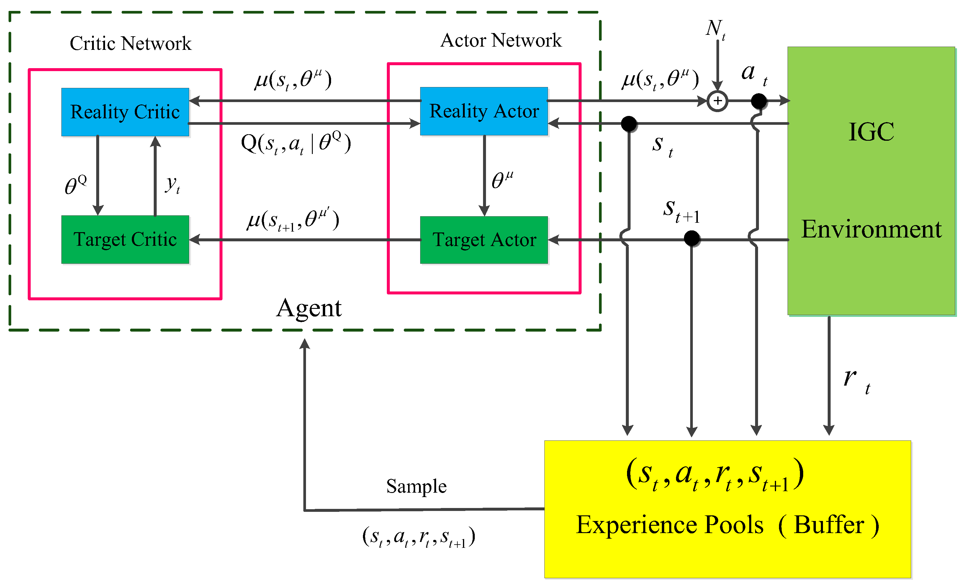
3.1. DDPG Algorithm Framework

A DDPG algorithm operates on Actor–Critic frameworks. Therefore, DRL consists of two parts: Critic-Network and Actor-Network. The Critic-Network consists of the Reality Critic and Target Critic, and the Actor-Network consists of the Reality Actor and Target Actor. Figure 2 shows the architecture of the proposed DRL -guidance-law system.

3.2. DDPG Algorithm Flow

The DDPG algorithm is based on the framework of a network with a Critic-Network and an Actor-Network with parameters denoted by θ Q and θ μ , respectively, where the Critic-Network performs the Q function calculation to obtain the Q value, Q s , a | θ Q , and the Actor-Network performs state-to-action mapping to obtain μ s | θ μ [28].
Algorithm 1: DDPG
1: Initialize critic network parameters θ Q and θ μ randomly
2: Initialize the respective Target-Network parameters θ Q θ Q , θ μ θ μ
3: Initialize the Experience Pools (Buffer) for storing empirical information
4: for episode = 1: Max Episode do
5:  Obtain the initialized state S 1
6:  for t = 1: Max Step do
7:    Select action a t = μ s | θ μ + N t , where N t is a Gaussian perturbation
8:    Execute a t   to obtain the corresponding reward r t and the next state s t + 1
9:    The tuple s t , a t , r t , s t + 1 formed by the above process is stored in Buffer
10:   Sample a random minibatch of N transitions s i , a i , r i , s i + 1 from Buffer
11:   Calculate the temporal-difference error σ i
      σ i = r i + γ Q ( s i + 1 , μ ( s i + 1 | θ μ ) | θ Q ) Q s i , a i | θ Q
12:   Update critic by minimizing the loss: L = 1 N i = 1 N σ i 2
13:   Update the Critic-Network using gradient descent:
        θ μ J 1 N i a Q s , a | θ Q | s = s i , a = μ s i θ μ μ s | θ μ | s i
14:   Update the target networks:
        θ Q τ θ Q + 1 τ θ Q
        θ μ τ θ μ + 1 τ θ μ
15:  end for
16: end for

4. Modeling the Reinforcement-Learning Problem

4.1. Reinforcement Learning Environment

To solve a 3D-integrated-guidance problem using DRL, the first step is to turn the problem into an RL framework. As the basis of RL, the Markov decision process (MDP) is a theoretical framework for achieving goals through interactive learning. Therefore, the first step is to build the MDP for the 3D-integrated-guidance model. According to the equations in Section 2, the state space can be S = R , R ˙ , q y , q ˙ y , q z , q ˙ z , α , β , w z , w y , and the action space A = δ z , δ y . The agent continuously updates by interacting with the environment and generating action commands to obtain higher reward values.

4.2. Reward Function

The reward function can be a formal, numerical representation of an intelligence’s goal. The agent maximizes the cumulative and probabilistic expectation of the benefits of the scalar reward signal received by the intelligence. In solving 3D guidance-and-control-integration problems, the probability of a rocket successfully flying to the target under random initial setup conditions is extremely low. Moreover, the agent receives a small positive incentive for the limited amount of fragmentary learning. We constructed a reward function, considering the constraints in the guidance process. The scalar reward values are dispersed into a single step for each training segment, thus gradually guiding the missile toward the target. The definition of the reward function considers three aspects: the fin-deflection angle, line-of-sight angular rate, and miss distance.
(1) Fin-declination constraint
R 1 = k R 1 δ z 2 + δ y 2
Equation (10) represents a constraint on the control energy of the fin system. The magnitude of the fin-deflection angle directly quantifies the speed loss due to the induced drag. Therefore, energy consumption needs to be controlled when designing the reward function.
(2) Line-of-sight angle-rate constraint
R 2 = k R 2   q y ˙ 2 + k R 3 q y ˙ q y ¨                             ( q y ˙ q y ¨ < 0 ) k R 2   q y ˙ 2                                                                 ( q y ˙ q y ¨ 0 )
R 3 = k R 2 q z ˙ 2 + k R 3 q z ˙ q z ¨                                             ( q z ˙ q z ¨ < 0 ) k R 2   q z ˙ 2                                                                               q z ˙ q z ¨ 0  
To track the target in real time, the line-of-sight angle needs to be a constant. Thus, the line-of-sight angular rate should be near zero. Equations (11) and (12) represent constraints on the field of view of the guide head. Here, we consider the convergence factor of the target line-of-sight angular velocity proposed in this study. When q ˙ q ¨ < 0 , q ˙ decreases, the law of q ˙ with time approaches the transverse coordinate, the required usual overload of the trajectory reduces with q ˙ , and the path becomes flat, at which point q ˙ converges. When q ˙ q ¨ > 0 , q ˙ increases continously, the law of q ˙ with time deflects from the transverse coordinate, the required usual overload of the ballistic path increases with q ˙ , and the ballistic track becomes curved. Consequently, q ˙ divergences. Notably, q ˙ should converge for the missile to turn smoothly. The design of the reward function considers the convergence of the angular velocity of the line of sight, thus improving the training-convergence speed and the missile’s interception accuracy.
(3) Constraint of miss distance
R 4 = k R 4 R ˙
R 5 = k R 5                         (   R R 0 < 1 ) 0                             R R 0 1
R 6 = k R 6 1 R                   ( R < 1 m ) 0                                                     R 1 m  
Equations (13)–(15) are reward functions based on miss-distance quantities. Here, we designed the DDF to determine suitable performance results in the same episode. Thus, the agent further screens out the state quantity with the smallest miss-distance amount in a three-stage function. Equation (13) indicates that R_4 receives a negative bonus when the distance R between the missile and the target increases. This term decreases the distance between the missile and the target. Equation (14) indicates that a fixed reward is obtained when the ratio of the missile–target distance R to the initial distance R_0 is less than 1‰. Otherwise, R_5 is 0. Equation (15) indicates that the intelligence receives a larger reward as R approaches 0, provided R is within the interval (0,1).
The coefficients of the reward function mentioned above are presented in Table 1.
The final reward function is given by
R r e w a r d = R 1 + R 2 + R 3 + R 4 + R 5 + R 6
As the final reward function, the R r e w a r d of Equation (16) is the sum of the reward functions, thus ensuring that the reward functions satisfy the constraints simultaneously.

4.3. Training Scheme

During the training process, the agent continuously updates the policy parameters to maximize the cumulative reward value obtained by interacting with the environment and generating control instructions.
In this study, the physical process of a missile intercepting an incoming target is the training solution. To ensure that the final policy obtained by the algorithm has some generalization capability, the initial ranges of the state changes of the missile and incoming target are presented in Table 2.
The target-maneuver equation is expressed as
x t = V t 0 t + x t 0                                               y t = D v t s i n π / 5 t + y t 0 z t =   V t 0 t + z t 0                                                    
where V t 0 denotes the initial velocity of the target and x t 0 , y t 0 , and z t 0 denote the components of the initial position of the target on the corresponding x , y , and z axes in the inertial coordinate system, respectively. The x t , y t , and z t denote the components of the instantaneous position of the target on each axis in the inertial coordinate system. The D v t indicates the acceleration of the target. To express the random motion of the target, V t 0 and D v t vary and y t moves according to the sinusoidal law.

4.4. Creating the Networks

The Actor- and Critic-Networks consist of a fully connected neural network with one input, one output, and three hidden layers. The output of the Actor-Network is a fin-declination instruction, which is a bounded instruction. Therefore, the activation function of the output layer of the Actor-Network uses the tanh function. The output of the Critic-Network has infinite amplitude requirements. Therefore, the output-layer-activation function of the Critic-Network can be linear. The other hidden layers are the activation function of the Relu function, expressed as
R e l u s = s                   s 0   0                   s < 0  
The specific parameters of the network structure are presented in Table 3.
According to the control requirements, each training episode stops when any of the termination conditions are satisfied.
(1)
R < 1 m
(2)
R ˙ > 0
(3)
y < 1 m
Adjusting the hyperparameters has a more significant impact on the performance of the DDPG algorithm. The training hyperparameters used in this study are presented in Table 4.

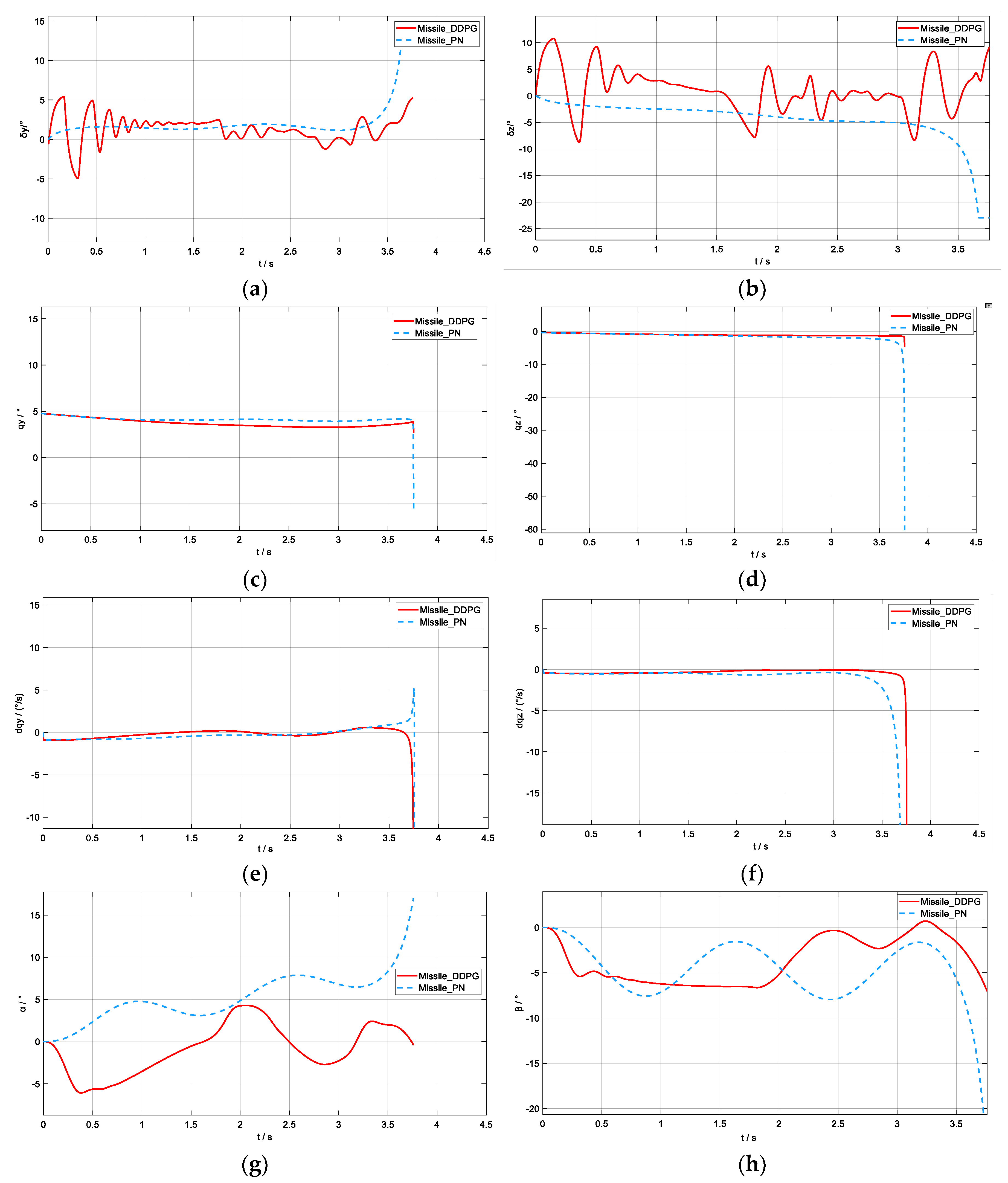
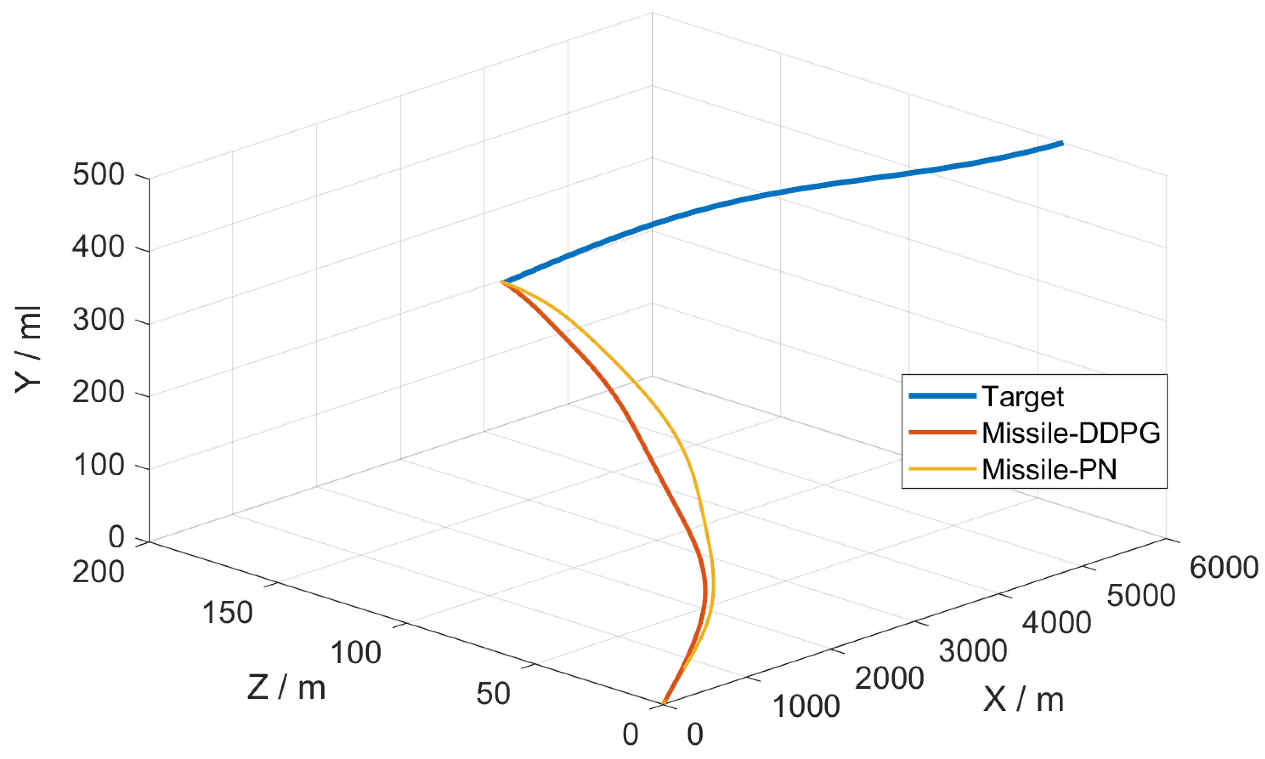
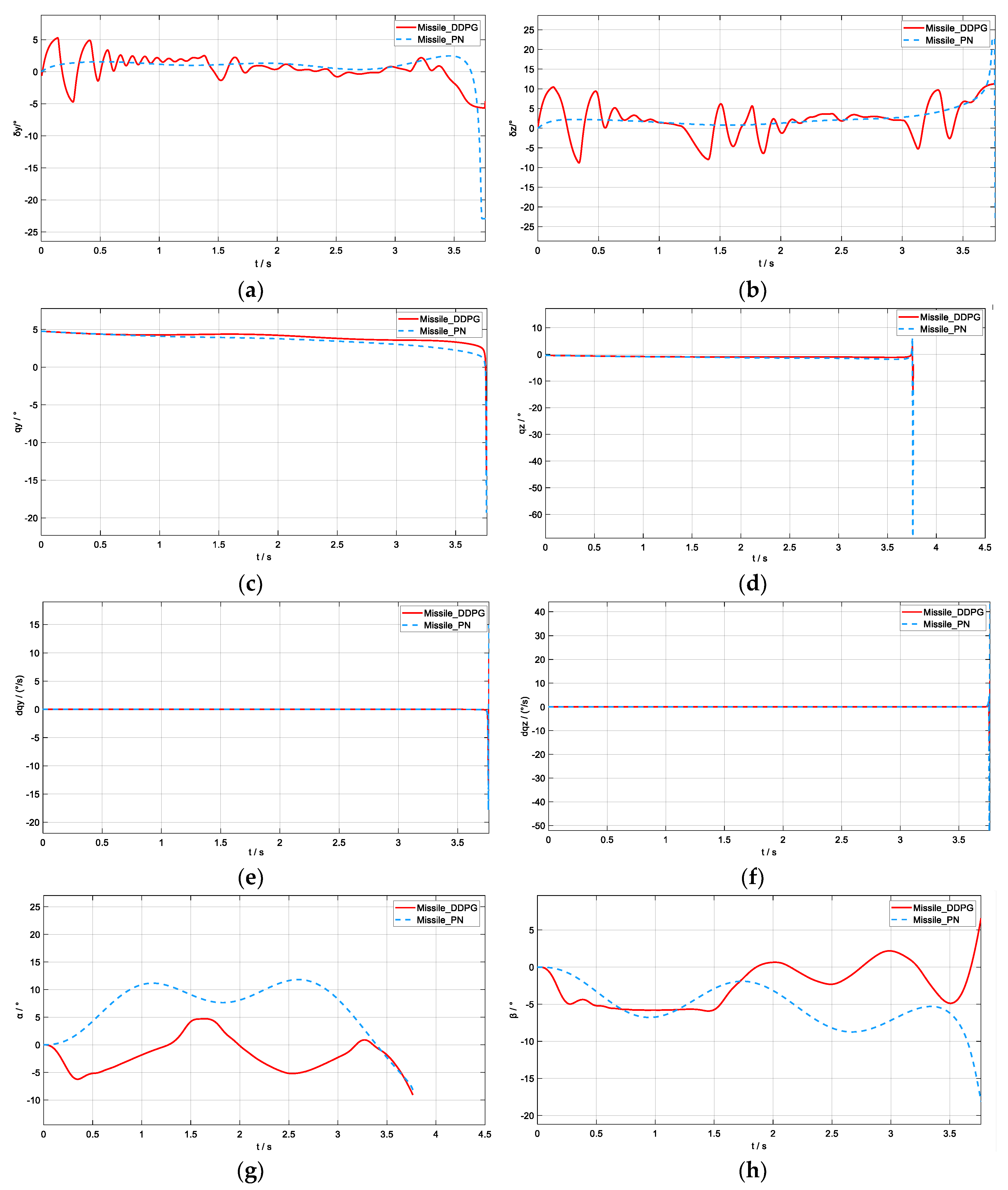
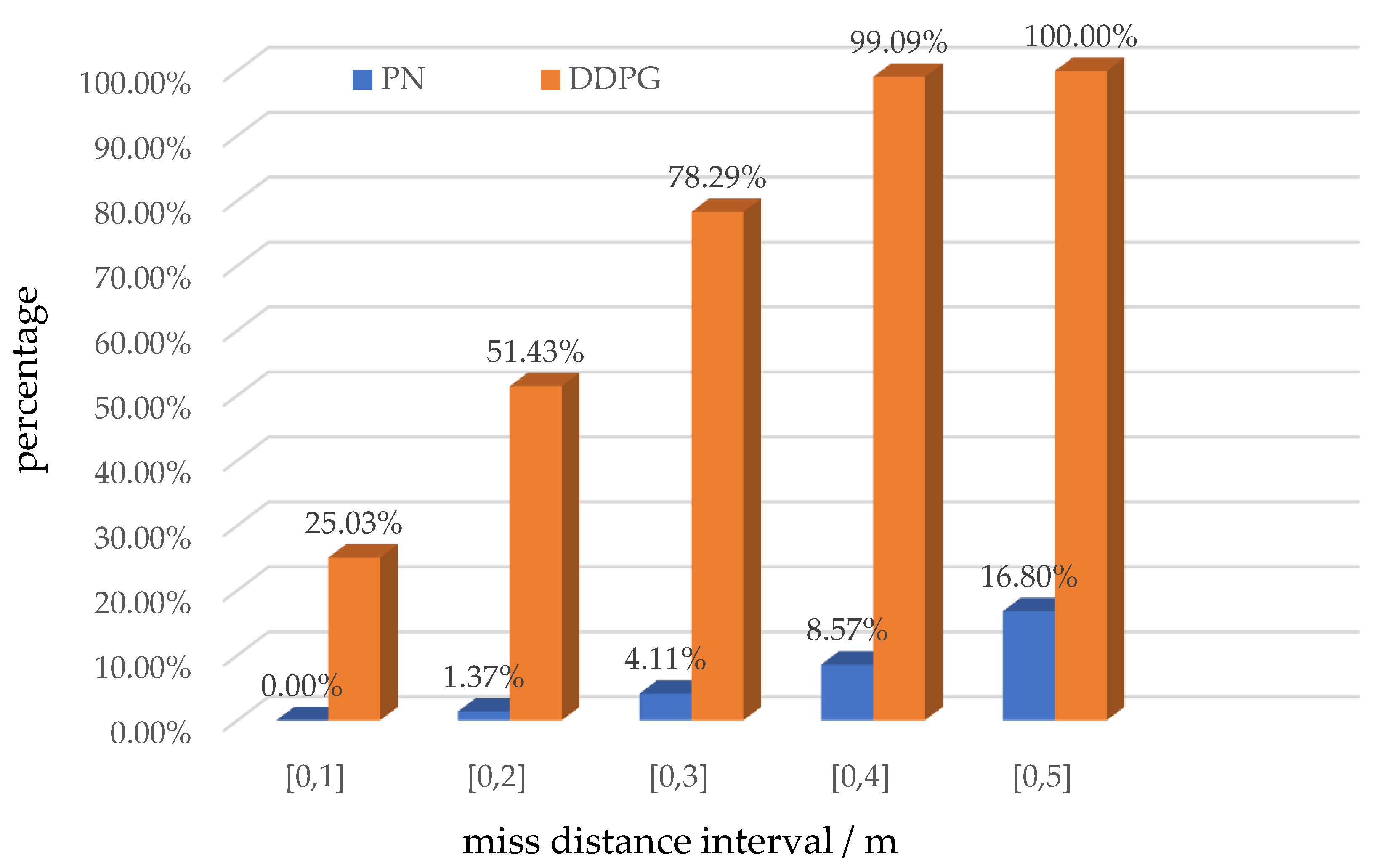
5. Simulation Results and Analysis

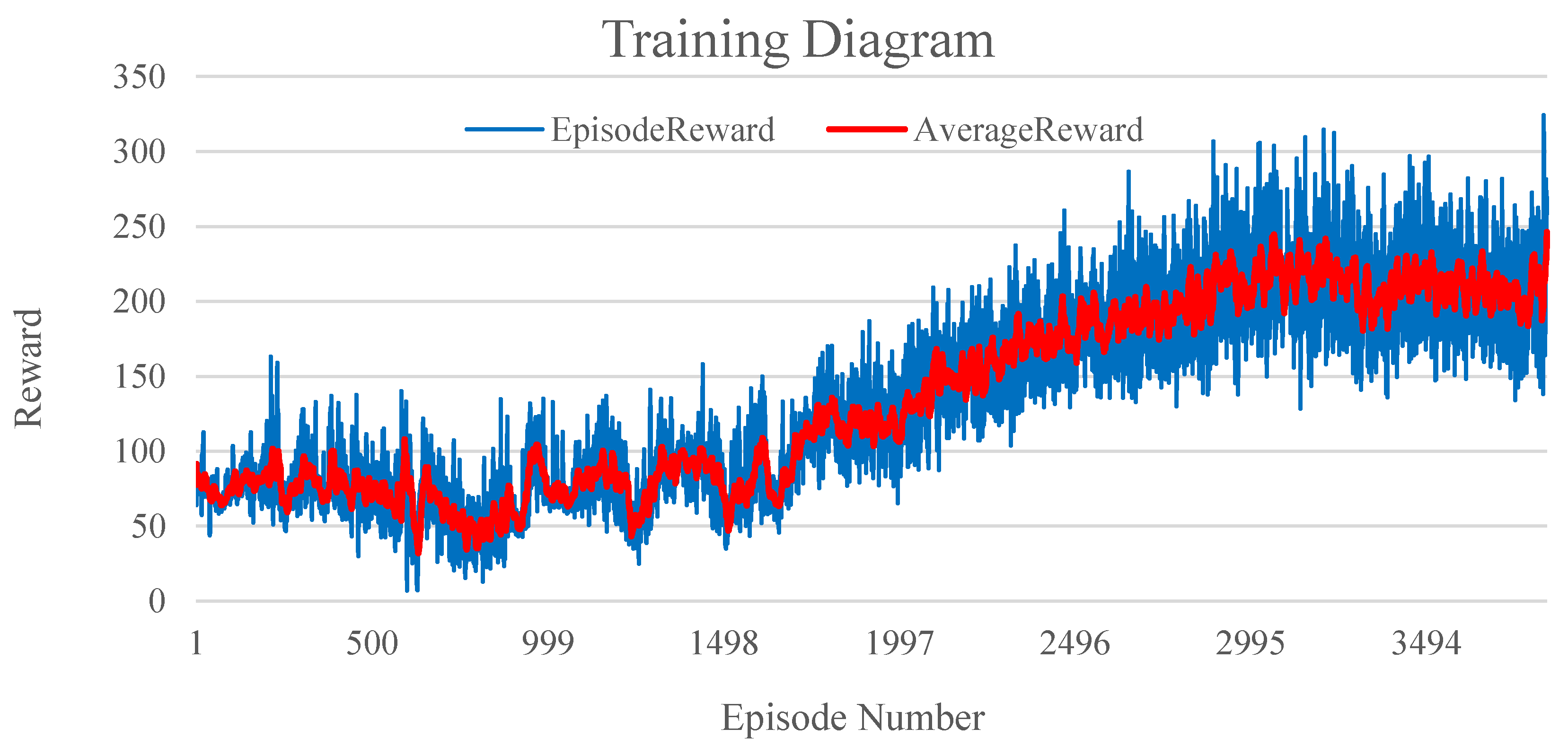
5.1. Training Results

According to the training scheme, the initial parameters of the missile and target were selected uniformly within the given range. The interception training of the incoming target attack fulfilled the preset requirements and satisfied the fin-deflection angle, field-of-view angle, and missile attitude constraints. The training curve is shown in Figure 3. The graph shows that the agent’s reward value was low in the pre-training phase and exhibited a slow upward trend as the number of training sessions increased. As the training progressed, the agent’s experience buffer contained significantly highly rewarded experience, causing the training-reward values to become fixed. The validation process must involve the examination of the strike accuracy and the speed at which the missile responds to the target.

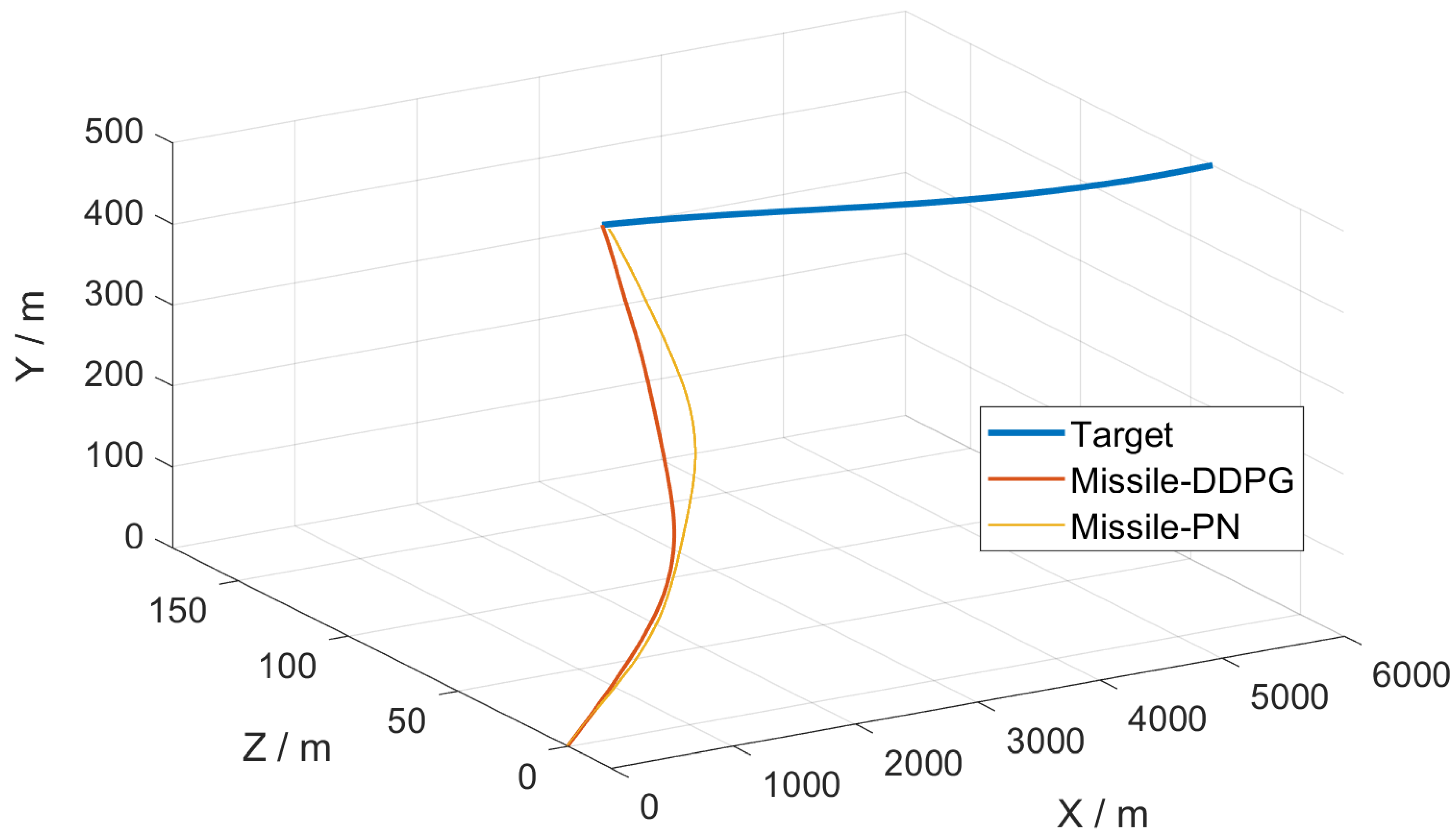
5.2. Simulation Verification

(1) Ballistic analysis
We saved the agents that satisfied the initial conditions and then converted these agents into integrated agents required for the simulation verification. We selected the exact initial conditions for the same model and compared the pure proportional-guidance law with the integrated DDPG algorithm proposed in this study. The pure proportional-guidance law implies that the missile-velocity vector is proportional to the angular velocity of the target’s line-of-sight rotation during an attack and expressed as
σ ˙ = K q ˙
where σ is the missile’s ballistic angle, q ˙ is the line-of-sight angular velocity, K is the scaling factor, and three is the scaling factor in this study.
Scenario 1. Scenario 1 is a training scenario. We selected the initial states of the missile and target randomly during the training and validation processes. Next, we chose the following scenario for analysis:
(1)
The target was at the farthest initial distance from the missile.
(2)
The target had the maximum initial velocity and acceleration.
(3)
The missile had the minimum initial velocity.
A 3D trajectory diagram of the missile–target interception process is shown in Figure 4.
The initial position coordinates of the target in this engagement scenario were ( X t 0 , Y t 0 , Z t 0 ) = 6000 , 500 , 40 , the initial velocity V t 0 = 700   m · s 1 , the initial acceleration D v t = 30 m · s 2 , the initial position coordinates of the missile were ( X m 0 , Y m 0 , Z m 0 ) = 0 , 0 , 0 , and the initial velocity of the missile is V m 0 = 900 m · s 1 . The missile–target-interception miss distance based on the DDPG algorithm was 0.66 m. In comparison, the distance based on the proportional guidance method was 2.56 m, further verifying the significant limitations of the proportional-guidance method in applying the guidance law for intercepting high-speed, highly maneuverable targets. Regarding the interception speed, the interception time of the proportional guidance method was 3.85 s. By contrast, the interception time of the DDPG algorithm was 3.76 s, indicating that the guidance law based on the DDPG algorithm can rapidly intercept targets.
To further analyze the performance of the guidance law based on the DDPG algorithm, the fin-deflection angle, line-of-sight angle, line-of-sight angular velocity, angle of attack, and yaw angle during the interception of the engagement mentioned in the above scenario are shown in Figure 5.
According to the fin-deflection curves, compared with the case based on the proportional-guidance method, the lateral and elevation fin-deflection angles based on the DDPG algorithm fluctuated more in the initial phase and then gradually stabilized with a controlled range of fluctuation. In the final guidance phase, compared with the proportional-guidance method, which benefits the dynamic flight in the final guidance phase, the DDPG algorithm did not show sudden changes in magnitude.
Figure 5c,d shows that the DDPG method kept the line-of-sight angle significantly smaller and the line-of-sight angular velocity closer to and around zero, indicating that the missile was always aimed at the target during the flight.
According to the angle-of-attack and sideslip curves shown in Figure 5g,h, the DDPG-algorithm-based guidance law enabled the missile’s angle of attack and sideslip to vary in a smaller range. The small overload required by the missile facilitated the regular operation of the instrumentation on board.
Scenario 2. Scenario 2 is a 30% positive pull-off of the missile’s aerodynamic parameters under the conditions of the training scenario. Additionally, it doubles the sine maneuver of the target in the y-direction, i.e., y t = D v t s i n 2 π / 5 t + y t 0 in Equation (17). The other conditions are the same as those in Scenario 1. Separate graphs of the missile–target-interception process are presented below.
A 3D trajectory diagram of the missile–target interception process of Scenario 2 is shown in Figure 6. In Scenario 2, the miss distance was 1.86 m for the DDPG-based algorithm and 4.21 m for the PN-based method. As shown in Figure 7c–f, the DDPG-based form exhibited a more stable state during the final guidance phase, with no significant sudden changes in angle or angular velocity. The curves in Figure 7g,h show that the range of variation in the angle of attack and sideslip of the missile based on the DDPG algorithm was smaller than when based on the purely proportional method. This benefited the stable flight of the missile and the regular operation of the equipment on board.
The DDPG-based IGC law demonstrated superior control performance to the pure proportional-guidance law in both Scenario 1 and Scenario 2. The feasibility and superiority of the proposed RL-based approach for solving the interception problem were verified.
(2) Analysis of miss distance
To fully validate the effect of the DDPG and PN algorithms on the miss distance, we selected the initial values of V m 0 , V t 0 , X t 0 , and D v t randomly within their respective intervals. The miss-distance distributions were verified using the DDPG-based and PN-based approaches. The test involved a total of 875 targeted trials. The statistical values of the miss distance are presented in Table 5, and the interval distribution of the miss-distance drawing is shown in Figure 8.
When V m 0 , V t 0 , X t 0 , and D v t varied within the training interval, the minimum value of the DDPG-based miss distance was 0.06 m, and the maximum was 4.17 m. The mean value was approximately 2 m, and the variance was approximately 1 m. The performances of all the metrics were better than that of the pure proportion-based miss distance. Figure 8 shows the distribution of the miss distance based on the DDPG-based and PN-based methods. Approximately all of the DDPG-based miss distances fell within the 5-meter interval. By contrast, the PN-based miss distance exceeded 1 m and, in most cases, exceeded 5 m. The test described above shows that the proposed guidance-law scheme has a high interception accuracy for maneuvering targets. Moreover, it can adapt to random changes in the initial parameters within a controlled range while ensuring the interception effect.
The information above refers to the targeting test for the RL training condition. The following information verifies the effect of the DDPG-algorithm and PN-algorithm guidance laws on the miss-distance quantity with uncertain aerodynamic parameters. The test acts on the parameters of Equation (9) with positive and negative pull bias, respectively. Table 6 shows the statistical miss-distance quantities based on the two algorithms.
Table 6 shows that the DDPG-based algorithm had a higher interception accuracy than the PN-based missile when the positive and negative pull-offs acted on the missile’s aerodynamic parameters. The miss distance gradually increased with increases in the pull-bias ratio. When pulling in the positive direction, the miss distances obtained based on DDPG were all within 1 m, whereas with the PN method, they exceeded 3 m. When pulling in the negative direction, the miss distance obtained based on the DDPG was approximately 1 m, whereas that based on the PN method was more than 10 m, and the maximum was 22 m. In addition, this test verified the generalizability of the DDPG algorithm.

6. Conclusions

This study designed a 3D integrated guidance-and-control law based on a DRL algorithm to address the difficulty of accurate modeling in high-speed-maneuvering-target-interception scenarios. First, we constructed a 3D integrated guidance-and-control-environment model in the RL framework. Next, the matching-state space, action space, reward function, and network structure were designed by comprehensively considering the miss distance, fin-deflection-angle constraint, and field-of-view-angle constraint. To comprehensively verify the proposed method’s interception performance, the training- and non-training-condition test scenarios were used to statistically simulate the DDPG and PN guidance laws. Numerous numerical-simulation results demonstrated that the reinforcement-learning-based IGC had high accuracy, strong robustness, and generalization ability in relation to the missile parameters and aerodynamic uncertainties. Through simulation verification, we realized that the convergence problem of the angular velocity of the target line of sight still allowed the study of the guide law. Moreover, some bizarre phenomena occurred in the random input of action.

Author Contributions

Conceptualization, W.W. and Z.C.; methodology, W.W. and M.W.; software, W.W. and X.L.; validation, Z.C., X.L. and M.W.; formal analysis, W.W.; investigation, W.W.; resources, W.W.; data curation, W.W.; writing—original draft preparation, W.W. and X.L.; writing—review and editing, W.W.; visualization, W.W.; supervision, M.W.; project administration, Z.C.; funding acquisition, Z.C. All authors have read and agreed to the published version of the manuscript.

Funding

This research received no external funding.

Data Availability Statement

The data that support the findings of this study are available on request from the corresponding author.

Conflicts of Interest

The authors declare no conflict of interest.

References

  1. Williams, D.E.; Friedland, B.; Richman, J. Integrated Guidance and Control for Combined Command/Homing Guidance. In Proceedings of the American Control Conference IEEE, Atlanta, GA, USA, 5–17 June 1988. [Google Scholar]
  2. Cho, N.; Kim, Y. Modified pure proportional navigation guidance law for impact time control. J. Guid. Control Dyn. 2016, 39, 852–872. [Google Scholar] [CrossRef]
  3. He, S.; Lee, C. Optimal proportional-integral guidance with reduced sensitivity to target maneuvers. IEEE Trans. Aerosp. Electron. Syst. 2018, 54, 2568–2579. [Google Scholar] [CrossRef]
  4. Asad, M.; Khan, S.; Ihsanullah; Mehmood, Z.; Shi, Y.; Memon, S.A.; Khan, U. A split target detection and tracking algorithm for ballistic missile tracking during the re-entry phase. Def. Technol. 2020, 16, 1142–1150. [Google Scholar] [CrossRef]
  5. Yanushevsky, R. Modern Missile Guidance, 1st ed.; Taylor & Francis Group: Boca Raton, FL, USA, 2007; pp. 12–19. [Google Scholar]
  6. Ming, C.; Wang, X.; Sun, R. A novel non-singular terminal sliding mode control-based integrated missile guidance and control with impact angle constraint. Aerosp. Sci. Technol. 2019, 94, 105368. [Google Scholar] [CrossRef]
  7. Wang, J.; Liu, L.; Zhao, T.; Tang, G. Integrated guidance and control for hypersonic vehicles in dive phase with multiple constraints. Aerosp. Sci. Technol. 2016, 53, 103–115. [Google Scholar] [CrossRef]
  8. Ai, X.L.; Shen, Y.C.; Wang, L.L. Adaptive integrated guidance and control for impact angle constrained interception with actuator saturation. Aeronaut. J. 2019, 123, 1437–1453. [Google Scholar] [CrossRef]
  9. Padhi, R.; Kothari, M. Model predictive static programming: A computationally efficient technique for suboptimal control design. Int. J. Innov. Comput. Inf. Control Ijicic 2009, 5, 23–35. [Google Scholar]
  10. Guo, B.Z.; Zhao, Z.L. On convergence of the nonlinear active disturbance rejection control for mimo systems. SIAM J. Control Optim. 2013, 51, 1727–1757. [Google Scholar] [CrossRef]
  11. Zhao, C.; Huang, Y. ADRC based input disturbance rejection for minimum-phase plants with unknown orders and/or uncertain relative degrees. J. Syst. Sci. Complex. 2012, 25, 625–640. [Google Scholar] [CrossRef]
  12. Mnih, V.; Kavukcuoglu, K.; Silver, D.; Rusu, A.A.; Veness, J.; Bellemare, M.G.; Graves, A.; Riedmiller, M.; Fidjeland, A.K.; Ostrovski, G.; et al. Human-level control through deep reinforcement learning. Nature 2015, 518, 529–533. [Google Scholar] [CrossRef]
  13. Li, S.; She, Y. Recent advances in contact dynamics and post-capture control for combined spacecraft. Prog. Aerosp. Sci. 2021, 120, 100678. [Google Scholar] [CrossRef]
  14. Gaudet, B.; Furfaro, R. Adaptive Pinpoint and Fuel Efficient Mars Landing Using Reinforcement Learning. IEEE/CAA J. Autom. Sin. 2014, 1, 397–411. [Google Scholar]
  15. Gaudet, B.; Linares, R.; Furfaro, R. Deep reinforcement learning for six degree-of-freedom planetary landing. Adv. Space Res. 2020, 65, 1723–1741. [Google Scholar] [CrossRef]
  16. Gaudet, B.; Furfaro, R.; Linares, R. Reinforcement learning for angle-only intercept guidance of maneuvering targets. Aerosp. Sci. Technol. 2020, 99, 105746. [Google Scholar] [CrossRef]
  17. Wu, M.-Y.; He, X.-J.; Qiu, Z.-M.; Chen, Z.-H. Guidance law of interceptors against a high-speed maneuvering target based on deep Q-Network. Trans. Inst. Meas. Control 2020, 44, 1373–1387. [Google Scholar] [CrossRef]
  18. He, S.; Shin, H.-S.; Tsourdos. Computational missile guidance: A deep reinforcement learning approach. J. Aerosp. Inf. Syst. 2021, 18, 571–582. [Google Scholar] [CrossRef]
  19. Pei, P.; Chen, Z. Integrated Guidance and Control for Missile Using Deep Reinforcement Learning. J. Astronaut. 2021, 42, 1293–1304. (In Chinese) [Google Scholar]
  20. Qinhao, Z.; Baiqiang, A.; Qinxue, Z. Reinforcement learning guidance law of Q-learning. Syst. Eng. Electron. 2019, 40, 67–71. [Google Scholar]
  21. Scorsoglio, A.; Furfaro, R.; Linares, R. Actor-critic reinforcement learning approach to relative motion guidance in near-rectilinear orbit. Adv. Astronaut. Sci. 2019, 168, 1737–1756. [Google Scholar]
  22. Fu, Z.; Zhang, K.; Gan, Q. Integrated Guidance and Control with Input Saturation and Impact Angle Constraint. Discret. Dyn. Nat. Soc. 2020, 2020, 1–19. [Google Scholar] [CrossRef]
  23. Kang, C. Full State Constrained Stochastic Adaptive Integrated Guidance and Control for STT Missiles with Non-Affine Aerodynamic Characteristics-ScienceDirect. Inf. Sci. 2020, 529, 42–58. [Google Scholar]
  24. Tian, J.; Xiong, N.; Zhang, S.; Yang, H.; Jiang, Z. Integrated guidance and control for missile with narrow field-of-view strapdown seeker. ISA Trans. 2020, 106, 124–137. [Google Scholar] [CrossRef]
  25. Jiang, S.; Tian, F.Q.; Sun, S.Y. Integrated guidance and control of guided projectile with multiple constraints based on fuzzy adaptive and dynamic surface-ScienceDirect. Def. Technol. 2020, 16, 1130–1141. [Google Scholar] [CrossRef]
  26. Zhang, D.; Ma, P.; Wang, S.; Chao, T. Multi-constraints adaptive finite-time integrated guidance and control design. Aerosp. Sci. Technol. 2020, 107, 106334. [Google Scholar] [CrossRef]
  27. Mnih, V.; Kavukcuoglu, K.; Silver, D.; Graves, A.; Antonoglou, I.; Wierstra, D.; Riedmiller, M. Playing Atari with deep reinforcement learning. arXiv 1312, arXiv:1312.5602. [Google Scholar]
  28. Lillicrap, T.P.; Hunt, J.J.; Pritzel, A.; Heess, N.; Erez, T.; Tassa, Y.; Silver, D.; Wierstra, D. Continuous control with deep reinforcement learning. arXiv 1509, arXiv:1509.02971. [Google Scholar]
Figure 1. Schematic of the interception space of missile.
Aerospace 10 00167 g001
Figure 2. Block diagram of the IGC guidance law based on RL.
Aerospace 10 00167 g002
Figure 3. Training diagram.
Aerospace 10 00167 g003
Figure 4. Missile–target 3D trajectory diagram (Scenario 1).
Aerospace 10 00167 g004
Figure 5. Ballistic curve: (a) and (b) are the lateral and elevated fin−deflection curves; (c) and (d) are the line−of−sight angles (y and z directions); (e) and (f) are the line−of−sight angular velocities (y and z directions); (g) and (h) are the angle−of−attack curve and sideslip−angle curve, respectively (Scenario 1).
Aerospace 10 00167 g005
Figure 6. Missile–target 3D trajectory diagram (Scenario 2).
Aerospace 10 00167 g006
Figure 7. Ballistic curve: (a) and (b) are the lateral and elevated fin−deflection curves; (c) and (d) are the line−of−sight angles (y and z directions); (e) and (f) are the line−of−sight angular velocities (y and z directions); (g) and (h) are the angle−of−attack curve and sideslip−angle curve, respectively (Scenario 2).
Aerospace 10 00167 g007
Figure 8. Distribution of miss distance.
Aerospace 10 00167 g008
Table 1. Coefficient values of the reward function.
k R 1 k R 2 k R 3 k R 4 k R 5 k R 6
0.10.020.20.12050
Table 2. Initial state values of the integrated 3D-guidance-and-control model.
Parameter NameMinMax
Target’s initial position X t 0 / m 40006000
Missile’s initial velocity V m 0 / m · s 1 9001100
Target’s initial speed V t 0 / m · s 1
(Negative direction)
5 00700
Initial acceleration in the y-direction of the target D v t / m · s 2 030
(Negative and positive
directions)
Table 3. Network structure.
Network LayerActor-NetworkCritic Network
Number of
Units
Activation
Function
Number of
Units
Activation
Function
Input layer10——12——
Hidden layer 164Relu64Relu
Hidden layer 2100Relu100Relu
Hidden layer 3100Relu100Relu
Output layer1tanh1Linear
Table 4. Training hyperparameters.
ParametersValueParametersValue
Maximum number of segments5000Sampling time 5 × 10 3
Actor learning rate 1 × 10 3 Noise variance 1 × 10 1
Critic learning rate 1 × 10 3 Noise-variance decay rate 1 × 10 6
Discount factor0.99Minimum sample size64
Target network smoothing factor 1 × 10 3 Experience buffer size 1 × 10 6
Table 5. Miss-distance statistics.
AlgorithmMinMaxAverageVariance
m m m m 2
DDPG0.064.171.971.08
PN1.3717214.1617.11
Table 6. Statistics of miss distance with changing aerodynamic parameters.
Change Mode and
Percentage
Positive Pull-OffNegative Pull-Off
10%20%30%10%20%30%
DDPG0.450.520.600.760.951.15
PN3.024.015.011.4218.0322
Disclaimer/Publisher’s Note: The statements, opinions and data contained in all publications are solely those of the individual author(s) and contributor(s) and not of MDPI and/or the editor(s). MDPI and/or the editor(s) disclaim responsibility for any injury to people or property resulting from any ideas, methods, instructions or products referred to in the content.

