1. Introduction
Rolling motion is the motion where a body flies at a constant pitch angle
α with respect to the freestream velocity vector, while undergoing a constant angular rotation
p about its longitudinal axis. An effect of this motion is the appearance of additional forces and moments, which add to the static forces and moments. Classical studies of the rotation of a body of revolution in crossflow led to the definition of the Magnus effect. This Magnus effect consists of the appearance of forces parallel and normal to the incoming flow when the body is rotating [
1]. Nielsen, when studying the missile’s motion, defines the Magnus forces and moments as those developing as a result of rolling at an angle of attack [
2]. For missiles, the Magnus effect of the body is usually small compared to that of the fins. The classical approach considers the Magnus side force linear with the reduced roll rate and the angle of attack. This is a good approach for low angles of attack [
2]. Using the Maple–Synge analysis, some researchers showed that there are in-plane and out-of-plane Magnus terms [
3]. They developed a model of the non-linear forces in rolling motion. Moreover, Liaño et al. used a strong non-linear model for the pitching moment to study the lateral motion of missiles [
4,
5]. Therefore, for rolling motion at high angles of attack studies, a question that arises is the appearance of non-linear effects similar to those described in those references.
In the last few years, with the availability of reliable computational fluid dynamics (CFD) codes, some numerical studies have been performed that reasonably compare the experimental data [
6].
Concerning missiles and axisymmetric bodies, a question arises regarding the Magnus effect at high angles of attack where the flow over an axisymmetric body is not symmetric, leading to a non-zero side force at zero spin rate [
7,
8,
9,
10,
11,
12,
13]. Additionally, the roughness induces a roll angle effect on the side and normal forces, and therefore on the moments [
7,
11]. Then, a prediction of the Magnus effect is difficult to assess because of the complex interactions due to the moving walls, roughness and shedding vortices that appear at the leeside. There is another concern prior to Magnus effect studies: a numerical study—conducted by the author of this paper and others—for an axisymmetric body at a low Mach number and high angles of attack led to the conclusion that roughness effect can be modeled by an unstructured grid, and the resultant calculations showed a roll angle dependence on the side of normal forces [
14]. This is an effect observed in wind tunnel tests for rough models [
10,
11,
12,
13]. Moreover, the resultant forces at several angles of attack were different depending on the roughness of the body and resembled either a structured grid (a polished body) or an unstructured grid (a rough body). The numerical results of this study (shown in reference [
15]) were in accordance with the experimental data of two models (polished and rough test models) of this axisymmetric configuration [
8].
This model was then used as a reference configuration for a CFD study of rolling motion at a low Mach number and high angles of attack. When making these CFD studies for rolling motion, a similar unstructured grid used in the previous numerical studies was used. The way to proceed for obtaining a numerical solution is to use the concept of dynamic meshes. The body and a cylinder that covers the body move with the prescribed roll velocity. This domain moves its boundaries relative to another fixed domain. In this particular domain, the nodes move rigidly in the given dynamic mesh zone. This is a sliding mesh, a particular case of a dynamic mesh. The interfaces between the fixed and the moving domains have to be treated such that they are connected at each time step during the transient calculation. The interfaces must be in contact with each other if fluid is able to flow from one domain to the other. The fluid motion is solved in an inertial reference frame [
16].
Then, at high incidence, there is not only an asymmetric flow, and therefore, a non-zero side force, but also a roll angle-dependent side force. The reason is that roughness triggers convective instability, which adds to global instability. The global instability leads to a bi-stable solution with either a positive or negative side force, each one a mirror of the other solution. The roughness effect activates the additional convective (or spatial) instability, which modifies the flow, particularly in the nose region, leading to rolling angle-dependent side forces and normal forces. The absolute values of the side force may vary significantly. One solution at a prescribed roll angle may have a side force that is 50% larger than that at another roll angle [
9,
10]. Therefore, the solutions between a polished model—with very low roughness—and a rough model may be very different. This effect has not only been observed in experimental tests [
8,
10] but has also been reproduced in numerical calculations [
14,
15]. The angle of attack for the onset of asymmetry is lower if the model has a large roughness. Then, the model in rolling motion at a certain angle of attack can develop a different flow pattern depending on whether a polished or a rough model is utilized.
In conclusion, a polished model with very low roughness can develop a rolling motion that is different depending on whether the angle of attack is larger or lower than the angle of attack for the onset of asymmetry. In the first case, the side force at zero spin is zero, i.e., the flow is symmetric. At higher angles of attack, where the side force at zero spin is either positive or negative depending on the initial perturbations, it is expected that the sign of the spin velocity will fix the sign of the resultant Magnus side force.
For rough models, it would be expected to have similar behavior, but in this case, the side forces at zero spin are rolling angle dependent, also in magnitude. Therefore, this may have an effect and non-symmetric solutions may be obtained when rolling at positive or negative spin velocities. This latter case has been numerically investigated from three different angles of attack. The first angle coincides with the angle of attack for the onset of asymmetry, while the other two angles of attack are larger and therefore, the flow at zero spin is asymmetric and roll angle dependent.
This paper describes the capabilities of CFD for obtaining reliable solutions that permit the analysis of the important non-linear effects that appear at high angles of attack, particularly at low roll rates.
Section 2 is related to the theoretical background regarding the model of the forces and moment coefficients and their derivatives.
Section 3 defines the configuration used for the theoretical calculations.
Section 4 describes the numerical simulation concerning the grids, methods and turbulence models employed. The results at zero spin for high angles of attack are described in
Section 5. The solutions at different roll rates and angles of attack for the test configuration are analyzed in
Section 6.
Section 7 is concerned with the Magnus effect in the forces. The conclusions of the study are given in
Section 8.
2. Theoretical Background
For a missile, a body axes Cartesian coordinate system is usually used. The origin is at the tip of the nose. The x-axis is parallel to the longitudinal axis of the body, positive in the tail direction. The y-axis and z-axis lie in a crossflow plane.
In general, a force or moment can be written as dependent on the values of
u,
v,
w,
p,
q,
r, i.e., the velocity components and the angular velocity components
. Making the components non-dimensional, we have:
being
the angles of attack and sideslip, respectively, and
is the velocity magnitude. The tangent angles of attack are defined as:
. For missile it is worth using the total angle of attack
and the bank or roll angle
. The relationship between these angles and the former angles is [
2]:
. Conversely, using
we have the relationship:
.
Additionally, for the tangent angles or attack : .
The components of angular velocities are made non-dimensional by . For a missile, the length is taken as the body’s maximum diameter and the velocity is the freestream velocity, .
For small angles and perturbations, and this can be performed with the total angle of attack and the angle of bank .
A linear approach for a force or moment for a missile configuration is defined by some authors [
17] as follows:
.
Nielsen defines Magnus forces and moments as those developing as a result of rolling at an angle of attack [
2]. The term
or
is normally defined as the Magnus effect term. The term
has been numerically estimated in several CFD studies, such as those carried out by Bhagwandin for a missile-type configuration [
18]. After a transient, the motion is periodic, and the side force coefficient
is computed as the averaged value in one rotation. This is conducted at several roll rates. The slope at each angle of attack is the Magnus side force spin derivative coefficient
, which permits calculating the Magnus side force derivative coefficient
when plotting versus the angle of attack.
In general, for a missile-type configuration formed by an axisymmetric body and a set of two, three or four fins, based on symmetry considerations, the Maple-Synge analysis can be used to model the force and moment coefficients and also their stability derivatives [
2]. However, this is not valid for high angles of attack due to flow separation. Moreover, at high angles of attack, the flow is asymmetric for an axisymmetric configuration due to the non-symmetric flow pattern from the tip on. Therefore, this theory is not appropriate to determine accurately the forces and moments coefficients, and particularly their derivatives, which are important for stability and control characteristics.
In reference [
3], a high-order model for a missile configuration (body and a set of fins) has been developed; the Magnus side force is characterized as:
The terms
are weighting factors, and the coefficients
are fin-alone coefficients. Details are given in the reference [
3]. In this model, there is not only a term for linearity with the reduced roll rate and angle of attack but also higher order terms for the angle of attack. Liaño et al. studied the influence on the free flight motion of a missile of a nine-order roll-dependent model of the pitching moment slope coefficient (
) [
4,
5]. Corresponding complex models can be derived for other coefficients, including the Magnus term. These models described in references [
3,
4,
5] show that there may be important terms not taken into account in a simple approach.
High-level CFD codes, which solve the unsteady Reynolds averaged Navier–Stokes (URANS) equations with complex turbulence models, have become reliable tools for computing the flow in regions where nonlinear effects are very important. Using CFD calculations, the forces and moments can be estimated, and their stability derivatives may be calculated using a finite difference approach or other methods, such as Kriging analysis. Additionally, nonlinear effects can be studied by analyzing the solutions. The numerical calculations presented herein have been performed using an axisymmetric configuration without fins, but with a large amount of numerical roughness and at a high angle of attack conditions.
4. Numerical Simulation
For the computations, URANS calculations with Reynolds stress turbulence models (RSM) combined with scale-adaptive simulation (RSM-SAS) have been employed. SAS can provide similar large Eddy simulation (LES) solutions, i.e., LES-like behavior in detached flow regions, while in stable flow regions, it recovers RANS performances [
20,
21,
22,
23]. The code used for the computations is the widely known ANSYS FLUENT
© [
16].
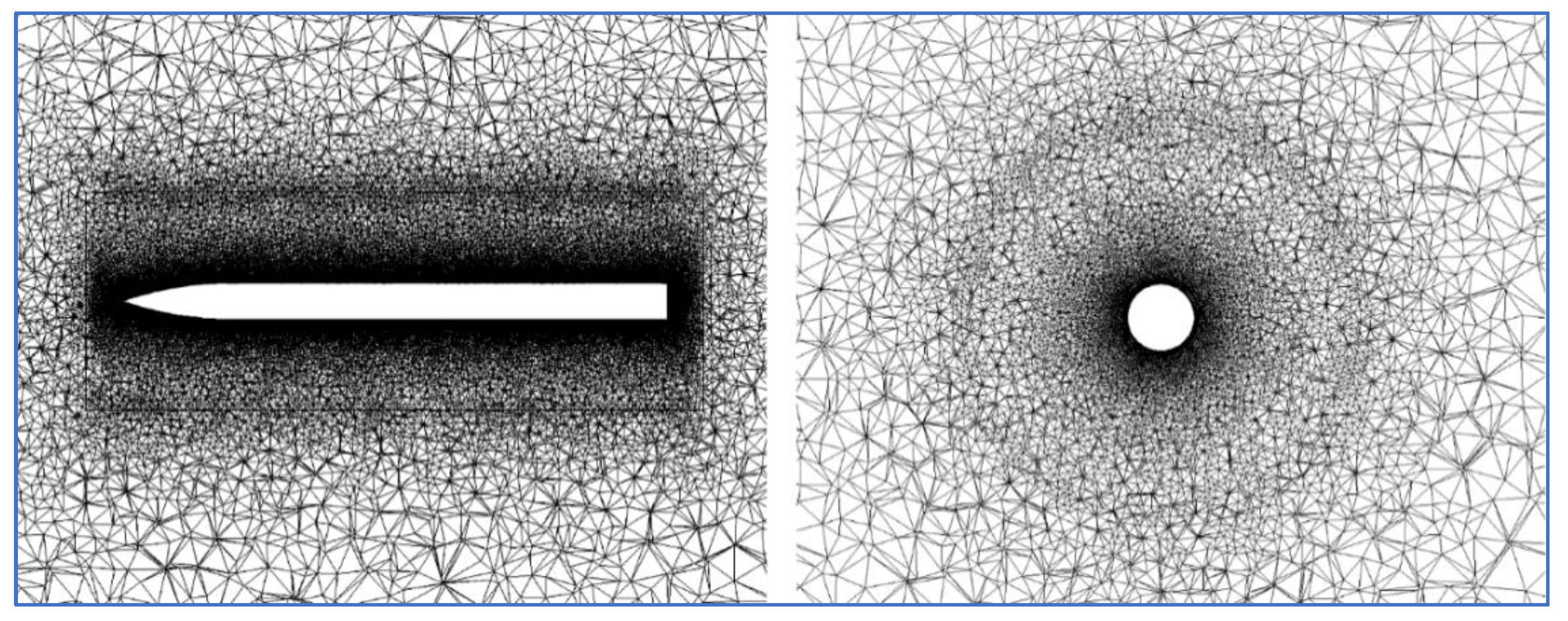
Structured axisymmetric grids were generated together with unstructured hybrid grids. For these latter grids, the surface grid cells are triangles, 48 prismatic layers were built in order to accurately resolve the boundary layer, and tetrahedral elements are in the outer domain. The total number of cells was approximately 16 million. The height of the first cell relative to the body surface was 1.0 × 10⁻⁵ (m). With this value, the y+ values were close to 1 in the whole-body domain.
This grid was generated such that the surface grid has geometrical irregularities, thus resembling a rough model. Before the calculations with this unstructured grid, an evaluation of the irregularities of the surface grid was conducted. In order to quantify these differences, a ‘numerical roughness’ is defined in the following manner:
First of all, as the test model is a body of revolution, the average radius at each
x/D section is defined as:
being
N the number of grid nodes. Then, the ‘numerical roughness’ at each section is calculated with the following expression:
. The measurements at the different
x/
D sections show results of ‘numerical roughness’ between 40 and 60×10
−6 m, i.e.,
rn/
D = 40–60 × 10
−6. This value is similar to that of a model used for testing the ogive-cylinder at several wind tunnels whose experimental data are shown in reference [
8].
In order to have the appropriate grid for studies of rolling motion, the concept of sliding mesh was used to allow the simulation of flow fields in the case of missile rotation: close to the body, a fine cylinder mesh is built such that it can rotate around the longitudinal axis if calculations with an angular velocity are performed. This cylinder may rotate with the corresponding body rotation, whereas the outer cylinder remains fixed. The solution in the nearfield is obtained in a moving reference frame, while in the outer field, an inertial reference frame is used. In the interface, proper interpolation of the fluxes must be done (for details, see reference [
16]).
A detail of this sliding mesh is given in
Figure 1.
A study with several values of time steps (Δt), ranging from to was conducted. It was checked that the first value of the time step was not sufficient. Large oscillations in the forces were obtained and the convective Courant number (CFL) values were large in zones of interest, when using these oscillations. Most of the solutions were obtained with this time step, but additional calculations were done using the finer value . Therefore, the spatial and time resolutions are adequate to run computations with the RSM-SAS turbulence model accurately, using the coarsest possible meshes and larger time steps, and taking advantage of the SAS capabilities for calculating massively separated flows and wakes. The computations were done in a cluster with 25 compute nodes, 24 cores per node. Four to eight nodes were used in each case. The typical computational time was approximately 48 h for one cycle of the rolling motion.
5. Flow Field at Zero Spin
The results obtained at the conditions of Mach number Ma = 0.2, Reynolds number Re = 2 × 10⁶ and angle of attack α = 45 degrees with two grids—structured and an unstructured grid—indicate an important effect of the roll angle on the forces if the unstructured grid is used. The influence of the roll angle is clearly due to the non-axisymmetric structure of the mesh—which leads to a numerical roughness—and to the surface roughness of a real body.
At a high angle of attack as large as 45 degrees where there is asymmetric flow, it is expected to obtain numerically asymmetric flow, but in accordance with the experimental data, the flow pattern must be a bi-stable pattern with two solutions, one mirroring the other with negative or positive side force but equal in magnitude as shown in experiments, (see [
8,
10]) provided the smooth model—structured grid—is used. The asymmetry is due to a global (or temporal) instability whose mechanism has been explained by several authors (see [
11]). The unstructured grid may provide a roll angle-dependent side and normal forces, thus indicating and additional convective instability effect, due to roughness.
For the calculations, first steady solutions were obtained, and then, a transient calculation with a small-time step of was used within a transient period of T = 4 s in the majority of cases. The calculations with the structured mesh at different roll angles showed a similar side force in magnitude; but in some cases, the sign differed. Therefore, the results obtained with the structured grid, which has a very low numerical roughness, seem to be in consonance with the experimental solutions, which at high angles of attack reproduce a bi-stable pattern of the side force, and a similar normal force, not dependent in magnitude on the roll angle.
It is remarkable to notice that a power spectral density analysis of the structured grid solution (within a period of
T = 4 s) shows energy content in the frequencies below 20 Hz. At higher frequencies, there is almost no energy content. The amplitude is one order of magnitude larger for the side force. The dominant frequency is 7.3 Hz for the side force. The Strouhal number is
, similar to the value 0.160 given as the experimental Strouhal in reference [
19].
The next step was to use the unstructured mesh and check if the ‘numerical roughness’ estimated previously was sufficient to lead to important differences in the flow pattern. Calculations at several roll angles were carried out.
The results of the averaged side and normal force coefficients for eight roll angles within a period of
T = 0.1 s are shown in
Table 1 and compared to the structured grid solution—which is independent of the roll angle in magnitude—and the experimental data obtained from reference [
19]. These experimental data are averaged values or data taken at one roll angle. There is no information about this in the documents (see [
8,
10,
19]). There are two roll angles for which the side force is negative. In one case (Φ = 270 deg.), the initial condition (steady solution) was of a similar sign, while in the other case (Φ = 45 deg.) there was a change of sign for the specular final solution with respect to the initial condition.
Due to the influence of the initial condition to end up with a positive or negative side force, the sign of the side force in
Table 1 is of little relevance, but it is important to observe the large differences induced by the roll angle on the absolute values of the side force coefficient
CY in the case of an unstructured mesh (that is, for an axisymmetric body with a rough surface).
An average roll angle side force coefficient can be calculated as:
N being the number of roll angles calculated. The use of absolute value is due to the two possible mirror solutions, of different signs and the same magnitude for each roll angle. This value is:
. Regarding the normal force coefficient, the variation with the roll angle is small but significant. The average normal force value is:
. This value is
. This normal force coefficient shows smaller variations, with a minimum value of 7.79 and a maximum of 8.44. Regarding the average value (8.13) there is a variation of 8%. The side force coefficient ranges from a minimum averaged value of 1.94 to a maximum of 3.22. These are variations of 50%. It is worth noting that experimental data corresponding to several tests (see references [
7,
10]) show variations up to 100% in the side force. The oscillation of the side force is larger than that of the normal force.
Then, the structure of the computational grid has a decisive role in the numerical simulations and the results could be extrapolated to experiments using bodies with different surface roughness. A structured axisymmetric grid resembles a very smooth body and the appearance of an asymmetric flow is due to hydrodynamic (global or temporal) instability. There is a bi-stable solution with two specific but otherwise similar flow field structures. However, a grid with large enough irregularities to resemble a rough model achieves different solutions approximately bounded by the two extreme values of the bi-stable solution.
There is another effect of the roughness: the angle of attack for the onset of asymmetry is lower for the rough model than for the smooth model (resembled numerically by the structured mesh). This angle was about 25 degrees for the smooth test model and 15 degrees for the rough test model at the conditions of Mach number Ma = 0.2 and Reynolds number Re = 2 × 10
6, according to references [
8,
10].
Regarding the unstructured grid solutions, the numerical values of the side and normal force coefficients at different angles of attack are given in
Table 2.
The experimental data showed an onset of asymmetry for an angle of attack below 20 degrees. At an angle of attack of 20 degrees, the side force is significant. According to Champigny [
8], the value for the angle of attack of the onset of asymmetry may be 12–15 degrees. According to this numerical simulation (
Table 2), this occurs between 20 and 25 degrees. This angle is smaller than that of the smooth body, indicating that the surface and flow irregularities trigger the appearance of asymmetric flow disturbances.
6. Rolling Motion
In the previous section, it was shown that at zero spin velocity at high angles of attack, there is a side force due to the asymmetric flow and that it is produced mainly by the existence of a global (or temporal) instability. Small perturbations on the initial flow or small irregularities lead to a bi-stable pattern of the side force solution (out of plane force). For the normal force, there is only one solution. Additionally, for an unstructured grid—which resembles a rough model—this side and normal forces are also roll angle dependent. The differences in magnitude for the side force coefficient at each roll angle are important. Therefore, for a theoretical point of view, it is different to choose as initial position one roll angle or other; but the spin motion will make that the effect of roughness must be reduced or averaged as the spin velocity increases. At a spin velocity of 2π rad/s (1 Hz), i.e., 360 degrees/s, the body is oriented at the same roll angle every 1 s. At a spin velocity of 20π rad/s (10 Hz), the body is oriented at the same position every 0.1 s. This roll frequency (10 Hz) is larger than the dominant frequency of 7.3 Hz for vortex shedding at the rear part of the body, as indicated by the power spectral analysis at zero spin. Then, some effect of roughness may appear at low spin velocities. Regarding the sign of the spin velocity, it is expected that the rolling with positive or negative angular velocity will lead to achieve a side force with the same sign, due to this movement perturbs the flow in one direction.
The calculations were performed on a non-rolled axis system. The origin is at the nose, and the x-axis is the longitudinal axis. In order to make the computations, the concept of sliding mesh, explained above, is used.
Prior to the calculations, a summary of the solution at zero spin velocity is given:
- i.
There is asymmetric flow with an important side force value at high angles of attack.
- ii.
For the unstructured grid, which has large numerical roughness, there is a dependence of the forces on the roll angle. There is an effect of convective (spatial) instability, which adds to the global (or temporal) instability due to the high angle of attack. The averaged value (for the different roll angles) at angle of attack α = 45 degrees is for the side force coefficient and for the normal force coefficient.
- iii.
The time step used is
. With this value, the Courant number (CFL) is close to 1 except in the boundary layer zone, where it reaches values up to 5. In order to obtain LES-like solutions, CFL must be of order 1. With the turbulence model employed (RSM-SAS) an important increment in time step would lead to a RANS solution. The results obtained for the calculations have captured a steady region at the nose and an unsteady flow region at the rear, which reproduce the main flow pattern observed in experiments [
24]. This flow structure is explained in Ref. [
14].
- iv.
The solutions at different angles of attack indicate an angle of attack for the onset of asymmetry of 20 degrees for the unstructured grid case. Additionally, the side force at 30 degrees is larger in magnitude than the side force at 35 degrees. Therefore, it was of interest to study previously the interval of angles of attack {35, 45} due to the evolution of the side force being linear with the angle of attack and both side forces being non-zero at zero spin velocity. The solution at the angle of onset for asymmetry is also of interest, as the flow is symmetric at zero spin.
Therefore, the calculations used in this rolling motion study were done using a similar time step, although a value of would be more accurate. However, the consequence would be an increment of the computing time by a factor of five times. A trade-off between flow accuracy and the number of solutions and calculations was performed.
In the next sub-sections, the calculations at angles of attack of 20, 35 and 45 degrees are shown. The first angle is the angle of onset for asymmetry. Then, at this angle, the flow is symmetric at zero spin.
- A.
Case 1: Angle of attack 45 degrees
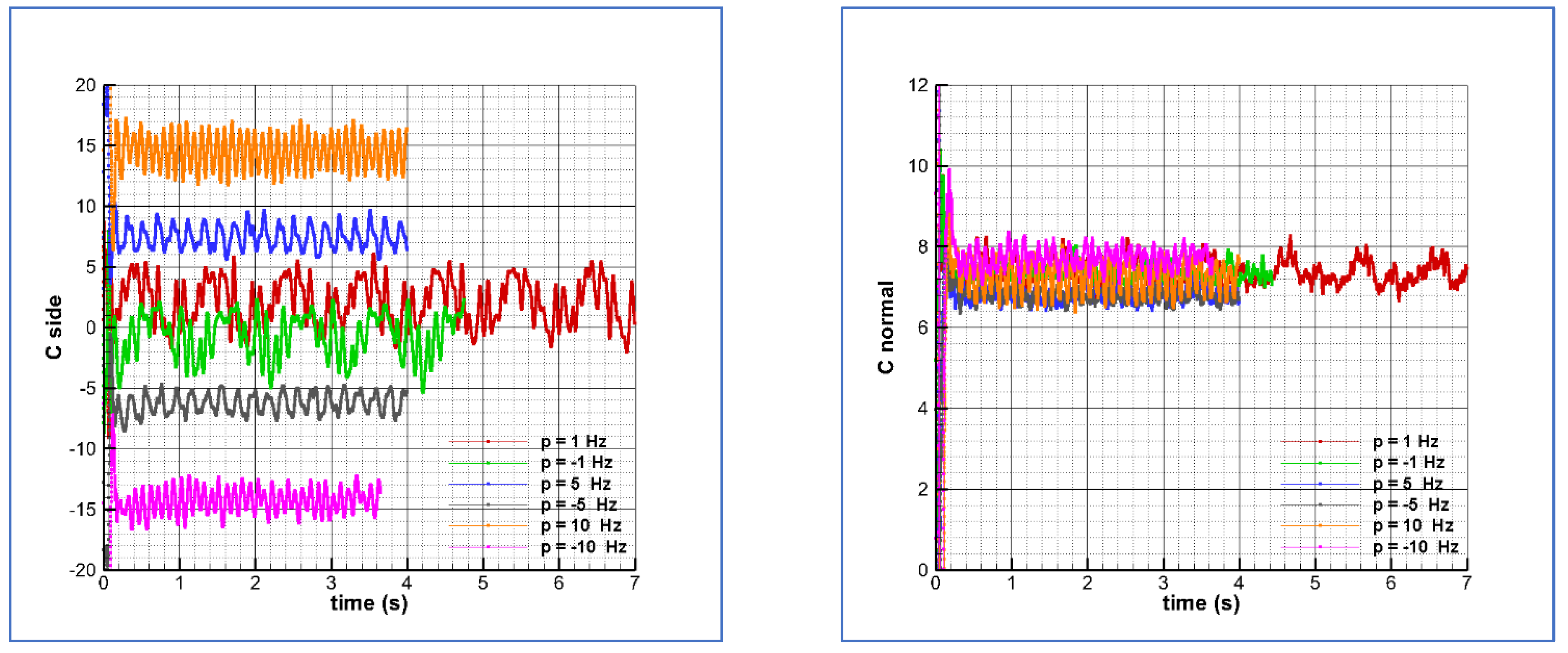
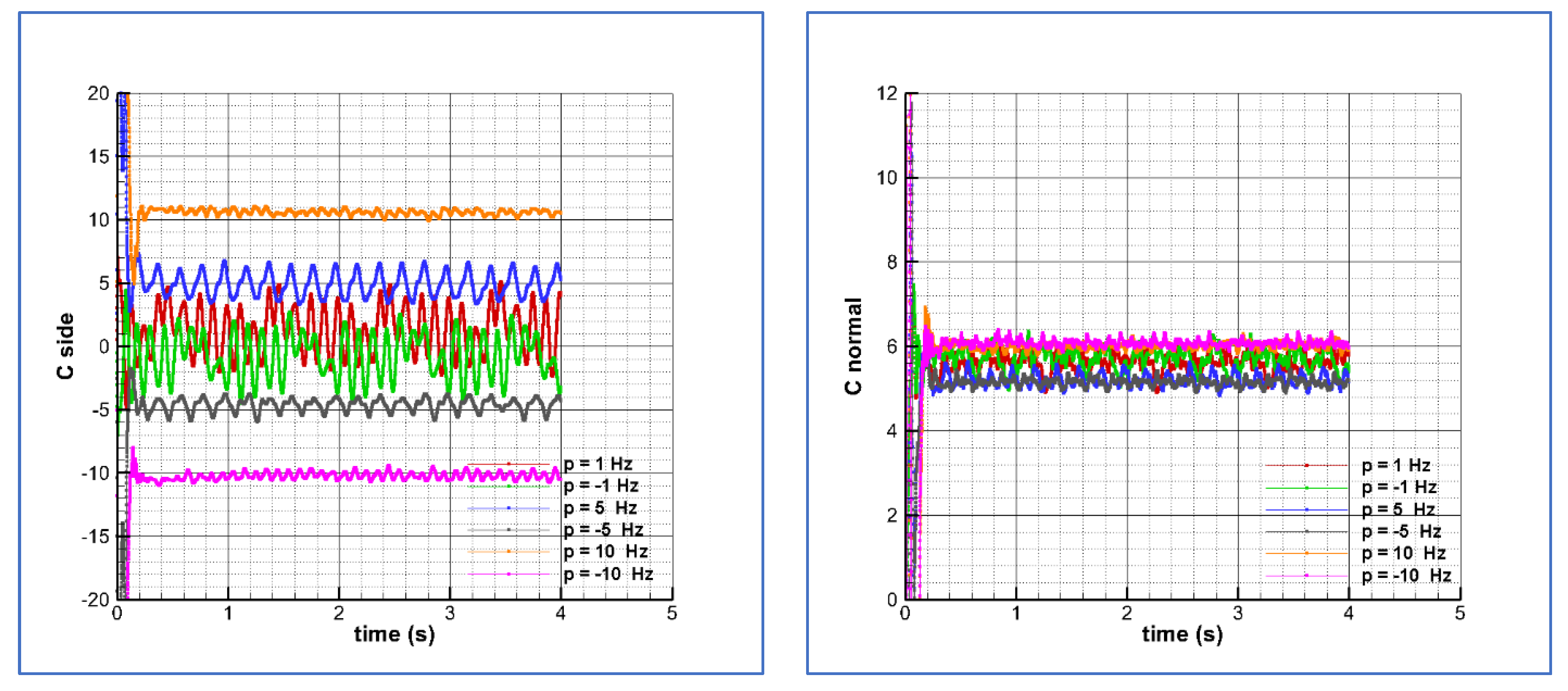
The time histories for the side and normal force coefficients at different roll velocities are plotted in
Figure 2. For the case of
p = 2π rad/s (1 Hz) the period of calculations was
T = 7 s. For most of the cases, the period used was
T = 4 s, i.e., 4 cycles. A periodical behavior was supposed in the last period. The calculations at zero spin led to a non-zero side force coefficient, which also depended on the roll angle. The average value (for the different roll angles) is
. Regarding the normal force coefficient, the average value (for the different roll angles) is
.
Average values within the calculated periods are represented in
Table 3. The standard deviations are included in the table. It can be observed that the standard deviation of the side force is larger than that of the normal force coefficient, as is usual at zero spin. Additionally, the minimum deviation occurs at the larger spin.
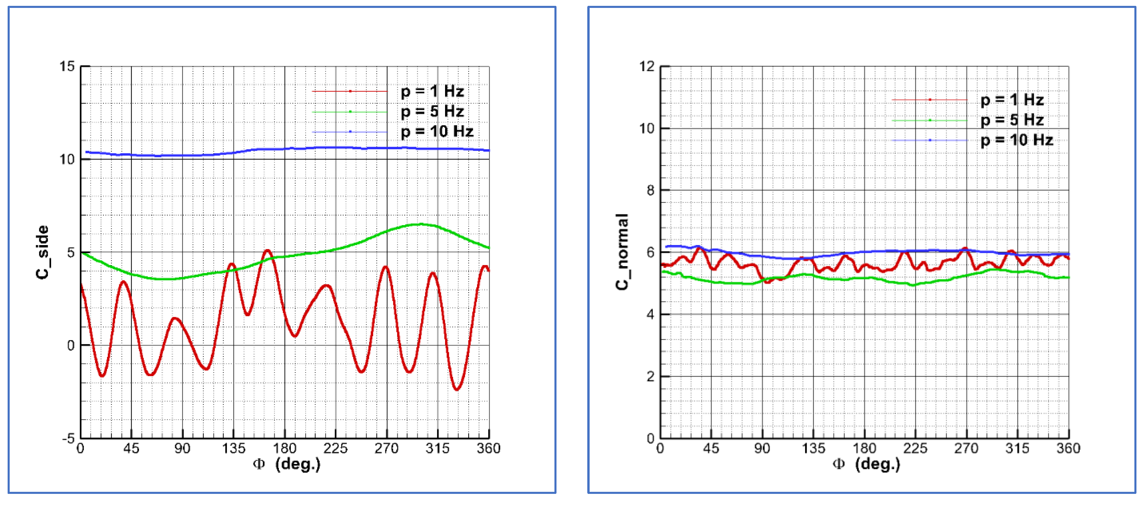
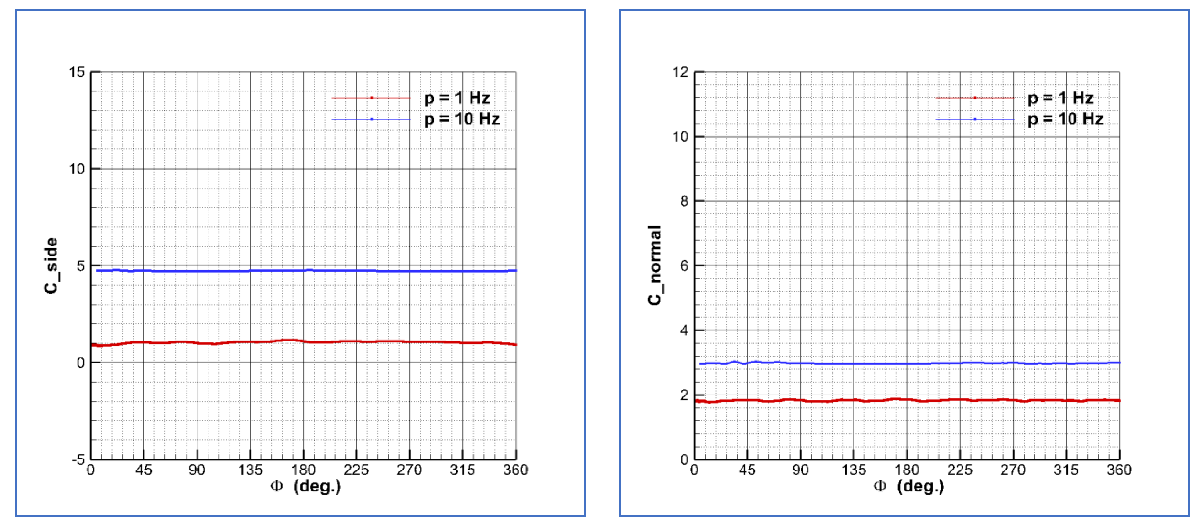
An illustrative figure of how these averaged values are obtained is shown in
Figure 3, which shows the side and normal force coefficients versus the roll angle within the last three cycles. Taking into account that at
t = 0 s the roll angle is zero, the roll angle is related to time and spin velocity as follows:
being
the time (s),
the spin velocity (rad/s) and
the number of cycles. It is worth noting that
T = 1 s for a complete cycle for
p = 2π rad/s, while
T = 0.2 s for
p = 10π rad/s and
T = 0.1 s for
p = 20π rad/s.
It can be checked that if p = 20π rad/s, the averaged side force coefficient is close to 14.5, but within a cycle, there is a minimum value of 12 and a maximum of 16. For the case of p = 2π rad/s, the averaged value is 2, but there are peaks of 5 and also negative values, up to −2. Regarding the normal force coefficient, this value is less roll dependent within a cycle, leading to a more constant value.
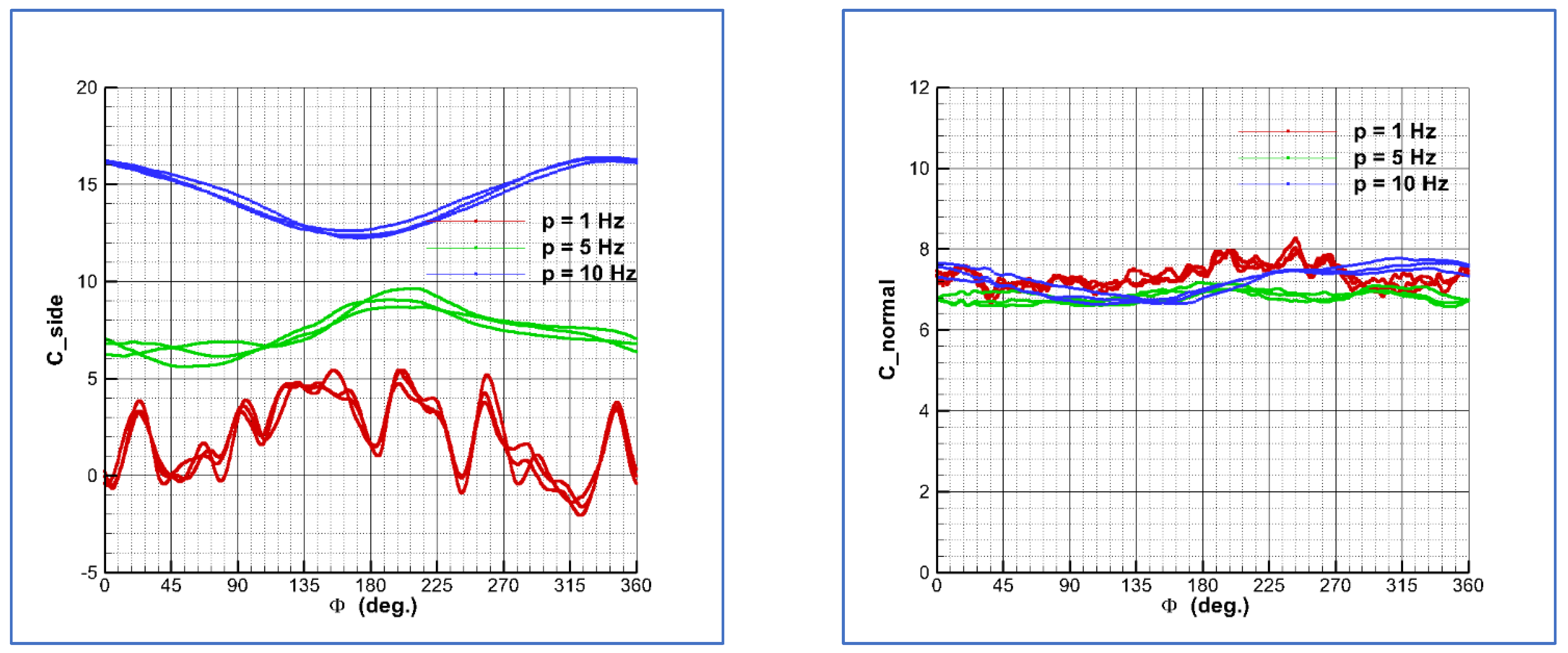
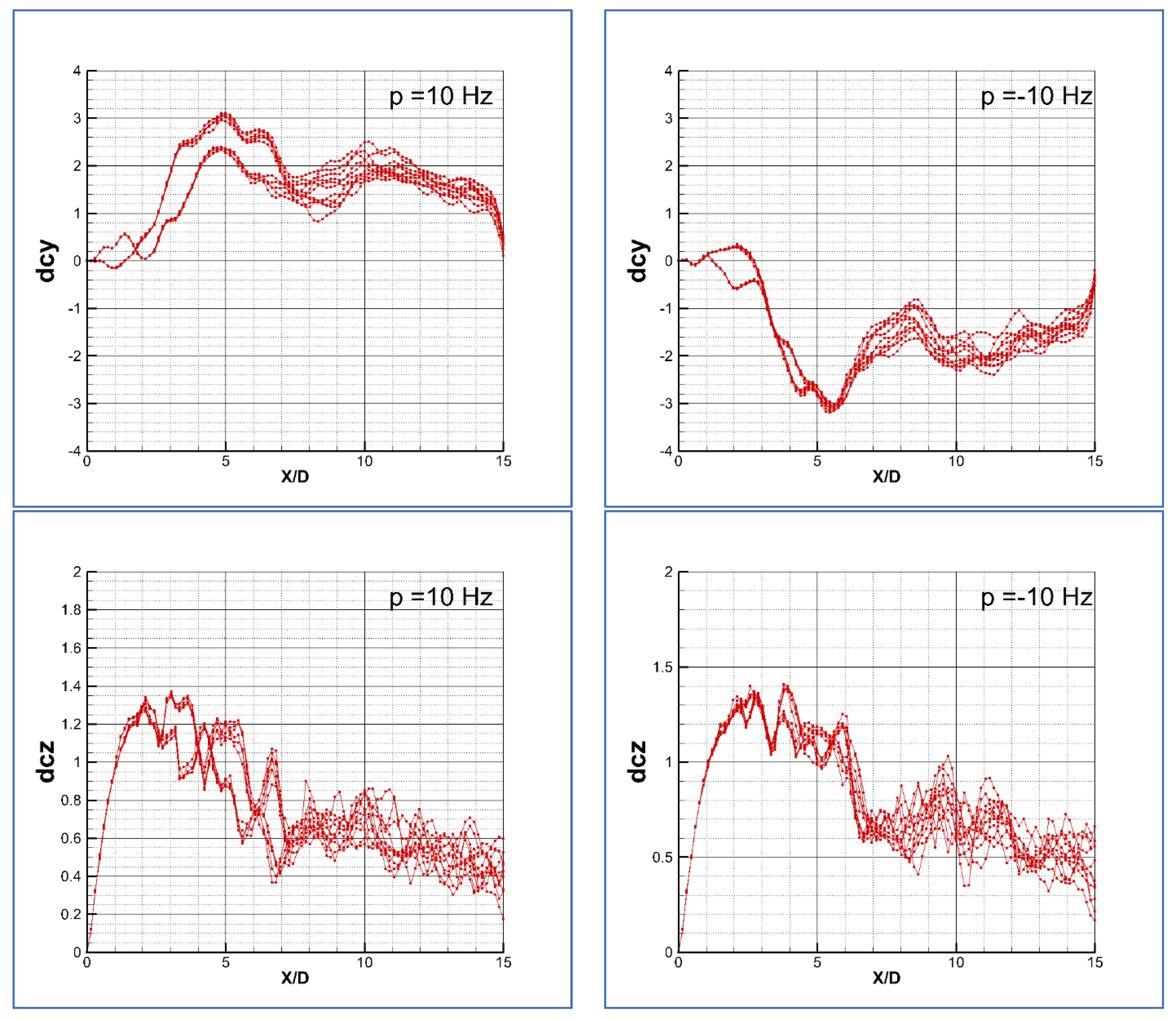
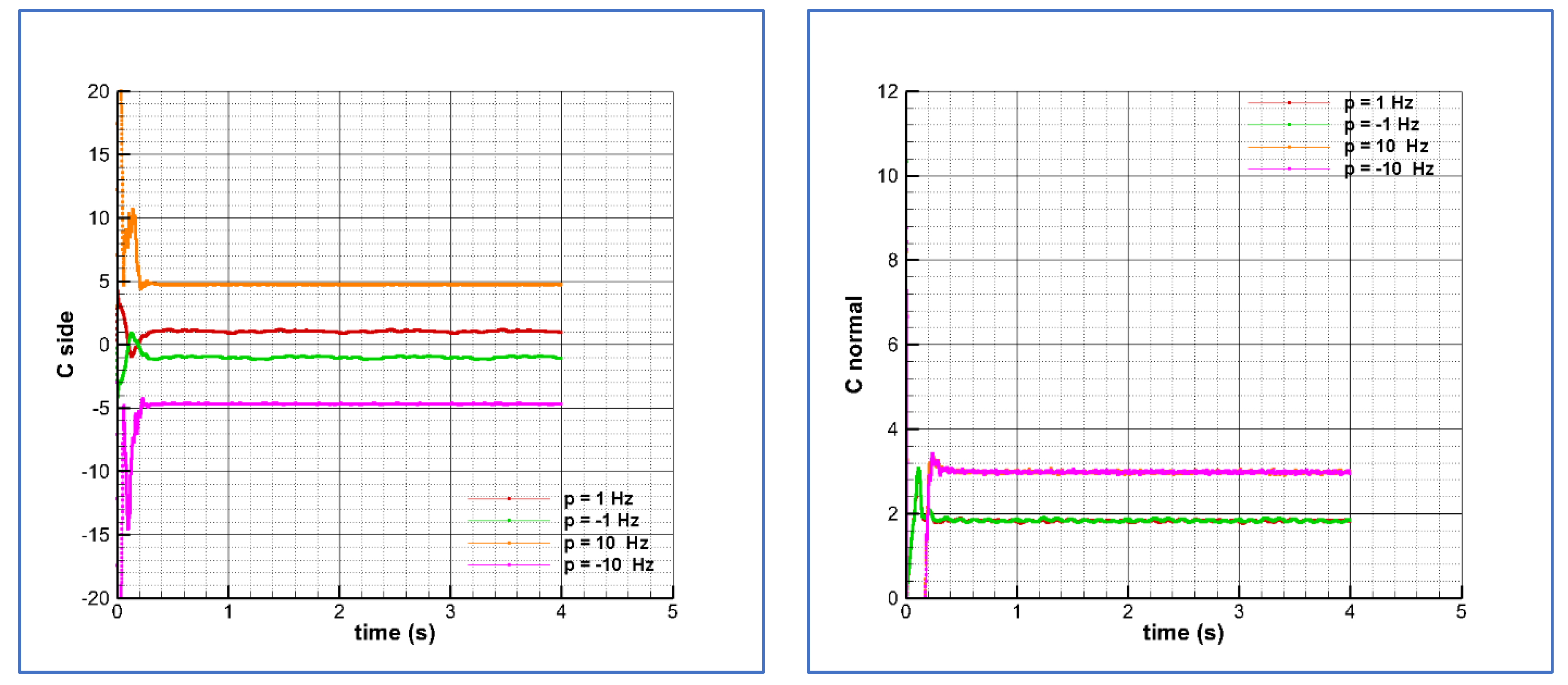
A good visualization of the persistence of the asymmetry is to look at the load curves for the longitudinal and lateral forces shown in
Figure 4. The plotted curves are taken each
within a period of T = 1 s, i.e., within a cycle. It can be checked that the side force at
p = −2π rad/s is not symmetric with respect to the solution at
p = 2π rad/s; moreover, the normal force coefficients are not equal for the cases of rotating at a positive spin velocity of
p = 2π rad/s or at a negative velocity of
p = −2π rad/s.
At zero spin, it was checked that there was an important effect of the numerical roughness, leading to the appearance of a convective (spatial) instability that produced a roll angle effect on the forces. When rolling at small spin velocities this effect seems to be still important, and the result is that at negative rolling the side force is negative but with an absolute value different to the value obtained at positive rolling with similar magnitude.
According to
Table 3, the global coefficients for the side and normal forces are similar, although not equal, for rolling at the higher spin calculated,
p = ±20π rad/s. The curves plotted in
Figure 5 for
p = ±20π rad/s are similar to the curves represented in
Figure 4 for
p = ±2π rad/s. In this case, the last five cycles are represented. The plots are curves within a period of
T = 0.5 s, taken each
. Again, it can be seen that the load curves are different depending on the sign of the roll velocity, indicating that there is still a bias effect, although the global values are more similar.
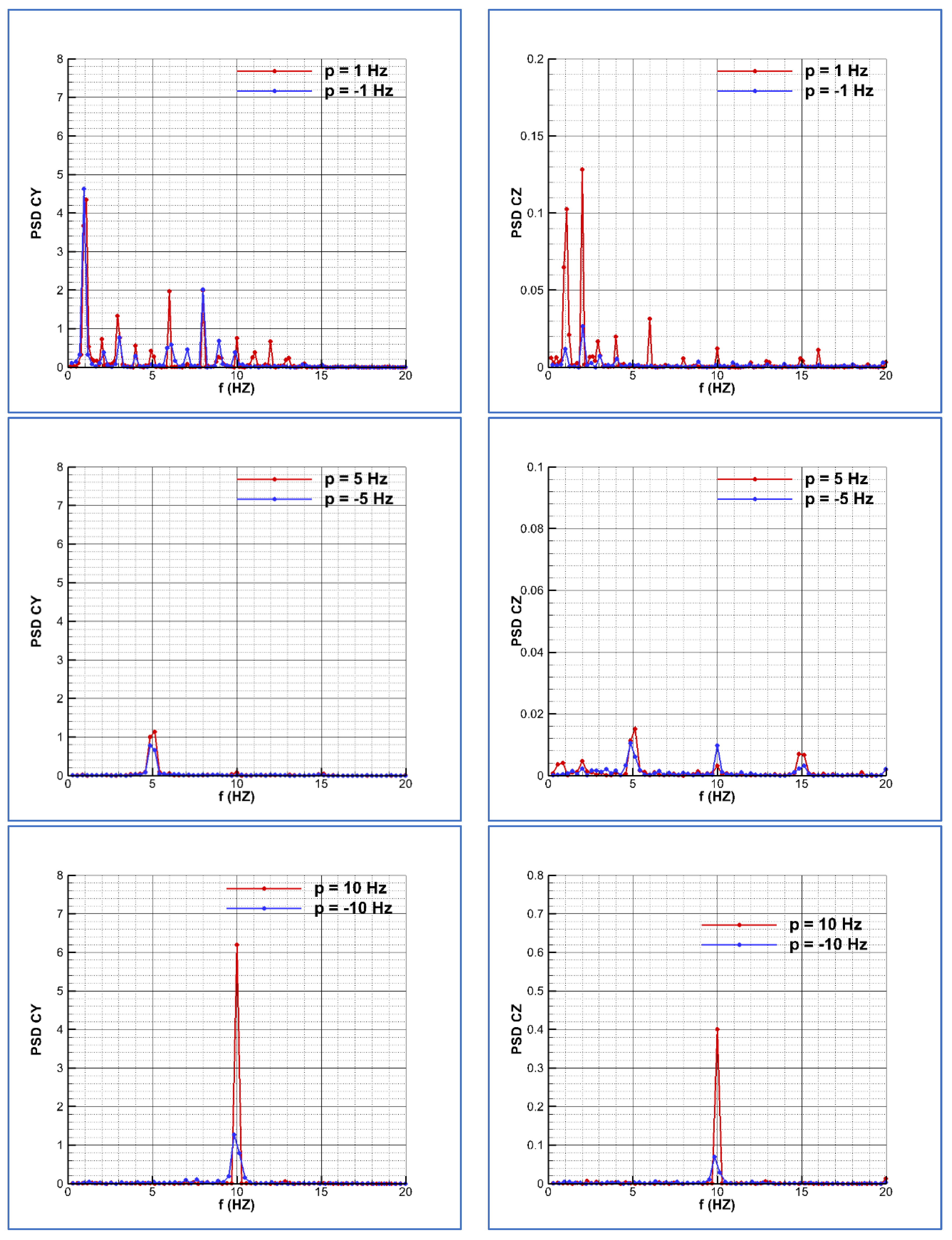
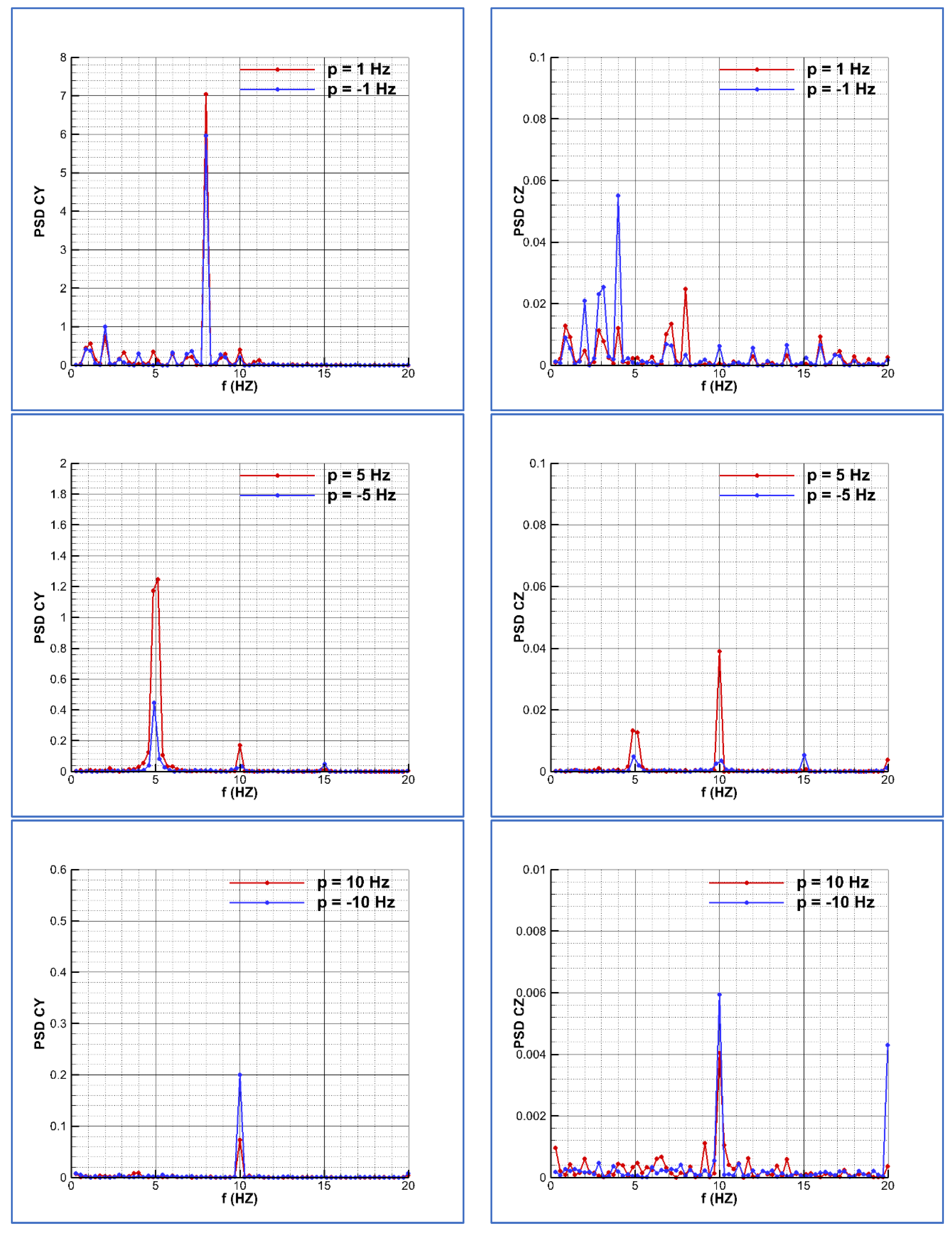
A power spectral density (PSD) analysis of the global forces within the periods of calculation for the spin velocities is given in
Figure 6. The solution in red color corresponds to the positive velocities and in blue color are the plotted negative velocities solutions. For the case of
p = ±20π rad/s (±10 Hz), this frequency of 10 Hz is the dominant frequency for both sides and normal force-velocity, but the magnitude is larger at the positive spin velocity than at the negative, indicating a non-symmetry in the solutions, as it has been checked looking at the load distributions (see
Figure 5).
Regarding the intermediate spin velocity, (p = ±10π rad/s) it can be checked that 5 Hz is the dominant frequency for the side force, but there is energy content at other frequencies multiple of this (10, 15 and 20 Hz) in the case of the normal force coefficient; and the magnitude is different depending on the sign of the spin velocity.
Regarding the lower spin velocity p = ±1 Hz, this is the dominant frequency for the side force, but there is energy content for frequencies up to 15 Hz. Again, the solutions are not symmetric. It can be seen that there is a large peak at 6 Hz for the positive spin, and a large peak at 8 Hz for the negative spin. It must be noted that at zero spin, the dominant frequency corresponds to 7.3 Hz. For the normal force coefficient, the dominant frequency is 2 Hz, the frequency double of the spin frequency. The magnitude is much larger at the positive spin than at the negative spin, indicating a bias effect, likely due to the surface numerical roughness.
- B.
Case 2: Angle of attack 35 degrees
At 35 degrees, the flow is asymmetric at zero spin, according to the calculations. The calculations for this angle were done only at the zero-roll angle. The effect of roll angle on the forces was not studied. However, it is likely that this effect exists. The time histories for the side and normal force coefficients at different roll velocities are plotted in
Figure 7. For all cases, the period used was
T = 4 s. The values of the side force at zero spin (positive and negative solutions) and of the normal force coefficient are given in
Table 2.
Averaged values within the calculated periods are represented in
Table 4. The standard deviations are included in the
Table 4. It can be observed again that the standard deviation of the side force is larger than that of the normal force coefficient, as is usual at zero spin. Additionally, the minimum deviation occurs at the larger spin.
Again, the value of the side force coefficient at p = 2π rad/s or p = 10π rad/s is larger than that of the negative spin velocities, p = −2π rad/s or p = −10π rad/s respectively. Therefore, there is an effect of the sign of the roll velocity, indicating a bias in the solutions.
An illustrative depiction of how these averaged values are obtained is shown in
Figure 8, which shows the side and normal force coefficients versus the roll angle within the last cycle. In this case, the solution is almost steady for the side and normal force coefficients at the larger spin velocity,
p = 20π rad/s. For an angle of attack α = 45 degrees, the solution was periodic. This curve indicates an increasing steadiness of the forces as the roll rate increases. The solution is neither roll angle nor time-dependent in a cycle.
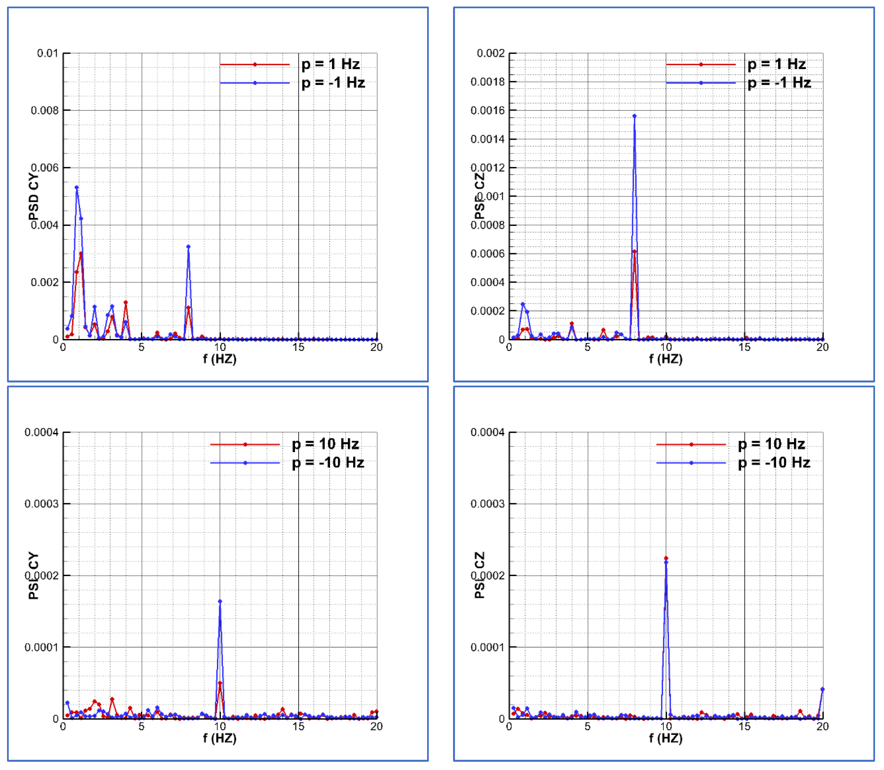
A power spectral density (PSD) analysis of the global forces within the periods of calculation for the spin velocities is given in
Figure 9. The solution in red color correspond to the positive velocities and in blue color are the plotted negative velocities solutions. For the case of
p = ±20π rad/s (±10 Hz) this frequency of 10 Hz is the dominant frequency for both side and normal force velocity, but the magnitude is larger at the negative spin velocity than at the positive, indicating a non-symmetry in the solutions. This trend is opposite to that observed at angle of attack α = 45 degrees. Regarding the intermediate spin velocity (
p = ±10π rad/s) it can be checked that 5 Hz is the dominant frequency for the side force, but there is content of energy at other frequencies multiple of this (10, 15 and 20 Hz) in the case of the normal force coefficient; and the magnitude is different depending on the sign of the spin velocity.
For the lower spin velocity p = ±1 Hz, the dominant frequency is not that corresponding to the spin velocity, but it is larger, at 8 Hz. There is an energy content of up to 10 Hz. The magnitudes are different depending is positive or negative the rolling velocity. Therefore, there is still a bias in the solutions.
- C.
Case 3: Angle of attack 20 degrees
Calculations at an angle of attack α = 20 degrees were also done. The flow at this angle is almost symmetric at zero spin. This angle corresponds to the angle of onset for asymmetry for this configuration and this grid with a certain level of numerical roughness. Therefore, in this case, the roll angle dependence of the forces is very small because the flow is basically symmetric. The time histories for the side and normal force coefficients at different roll velocities are plotted in
Figure 10. For all cases, the period used was
T = 4 s. The averaged values at zero spin are
and
.
An illustrative depiction of how these averaged values are obtained is in
Figure 11, which shows the side and normal force coefficients versus the roll angle within the last cycle. Looking at
Figure 10 and
Figure 11, it can be checked that the solution is steady for the side and has normal force coefficients at the two spin velocities.
Averaged values within the calculated periods are represented in
Table 5. The standard deviations are included in the
Table 5. It can be observed in this case that the standard deviation of the side force is very small. The solution is almost steady and symmetric: the solutions in terms of side force are similar in magnitude for both negative and positive spin velocities. The normal force coefficients are equal in magnitude, as well.
A power spectral density (PSD) analysis of the global forces within the periods of calculation for the spin velocities is given in
Figure 12. The solution in red color corresponds to the positive velocities and in blue color are plotted the negative velocities solutions. Although there are some differences depending on the sign of the spin velocity, it can be appreciated that the content of energy is very small compared to that of the solutions at the larger angles of attack (see
Figure 6 and
Figure 9).
7. Analysis of the Magnus Effect on the Global Forces
The data shown in
Table 3,
Table 4 and
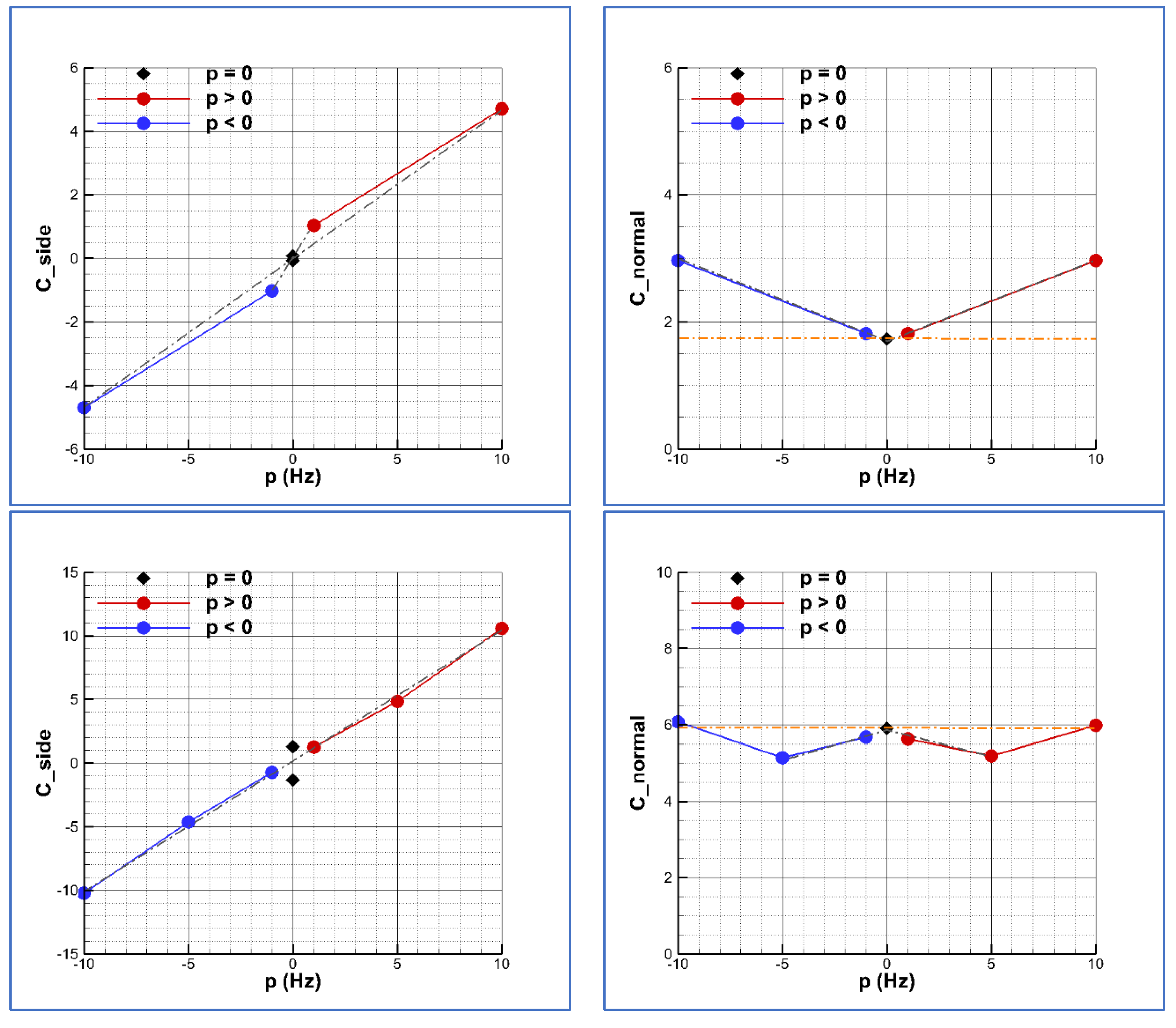
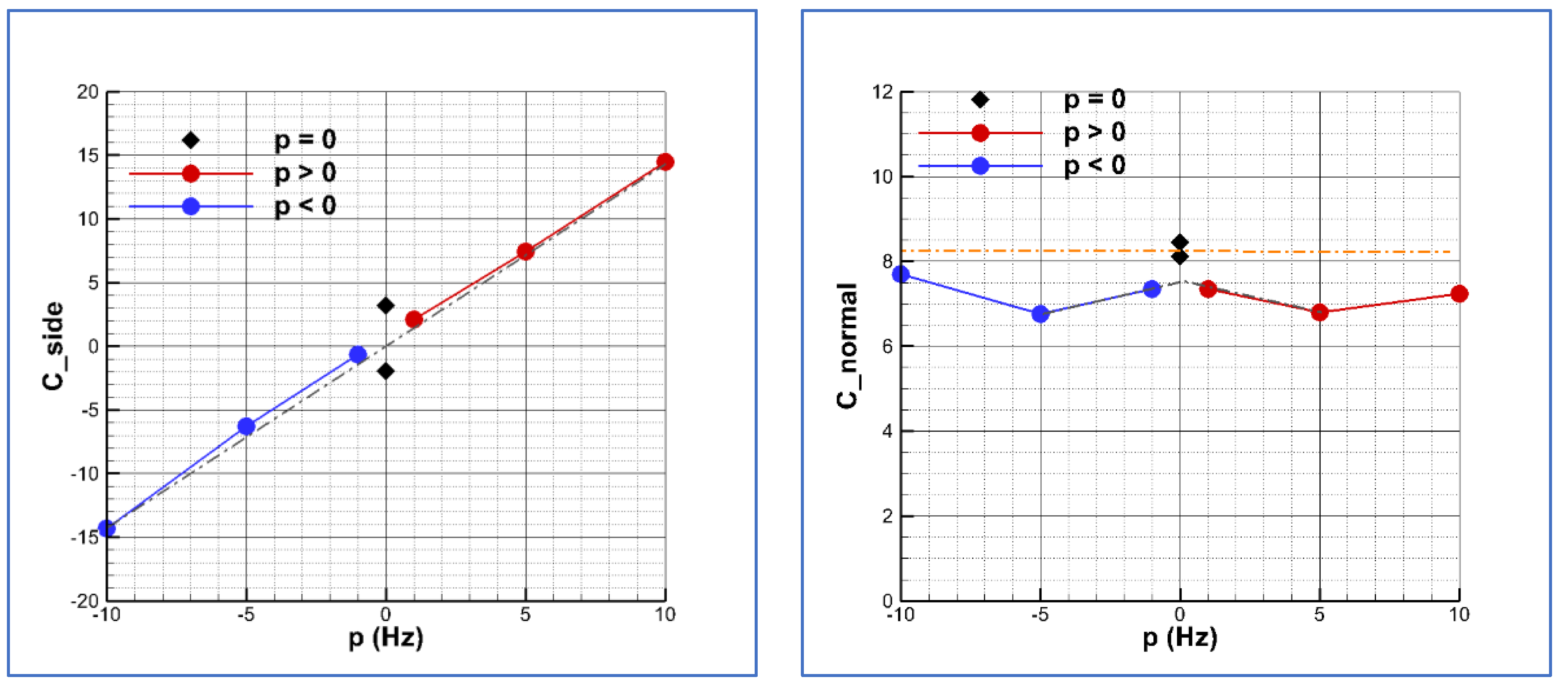
Table 5 regarding the averaged solutions for the side and normal force coefficients at the different angles of attack are plotted versus the spin velocity in
Figure 13. The blue symbols correspond to negative spin velocities, while the red symbols correspond to positive spin velocities.
The extreme solutions of the side force coefficient obtained at the larger spin velocity, i.e., p = ±20π rad/s, have been used to create a linear law (grey line), crossing the (0, 0) point. That means assuming symmetric flow at zero spin. For reference, the two possible solutions for the side force (positive or negative) obtained at zero spin calculations are plotted in black diamonds. For the lower angle of attack, this is zero because the solution is really symmetric at this angle. However, for the larger angles of attack, there is a non-zero side force at zero spin. The analysis of the first curves corresponding to α = 20 degrees indicates that the solutions at p = ±2π rad/s (±1 Hz) do not fit the linear law obtained with the extreme solutions. This indicates an effect that cannot be explained as a linear Magnus. Regarding the normal force coefficient, there is a very important linear Magnus effect. At p = 20π rad/s the normal force coefficient is almost 3. That means an increment of nearly 70% with respect to the zero-spin value (indicated as a reference constant orange dash-dot line in the figure).
Looking at the solution at α = 35 degrees, it can be seen that there is a small asymmetry in the solutions depending on the sign of the spin velocity and that the solutions at p = ±2π rad/s fit the linear law, but the solutions at p = ±10π rad/s are slightly out of this curve, indicating a non-linear effect. The behavior of the normal force coefficient is much more different to that of the curve at α = 20 degrees. The normal force coefficient decreases as the spin velocity increases up to p = ±10π rad/s and then starts to increase, reaching a similar value to that of zero spin (reference constant dash-dot line) at p = ±20π rad/s. The solutions at the larger angle of attack of α = 45 degrees reproduce the same behavior as that at 35 degrees. However, in this case, the asymmetry is still present at the larger spin velocities. The side and normal force coefficients have different magnitudes depending on the sign of the spin velocity.
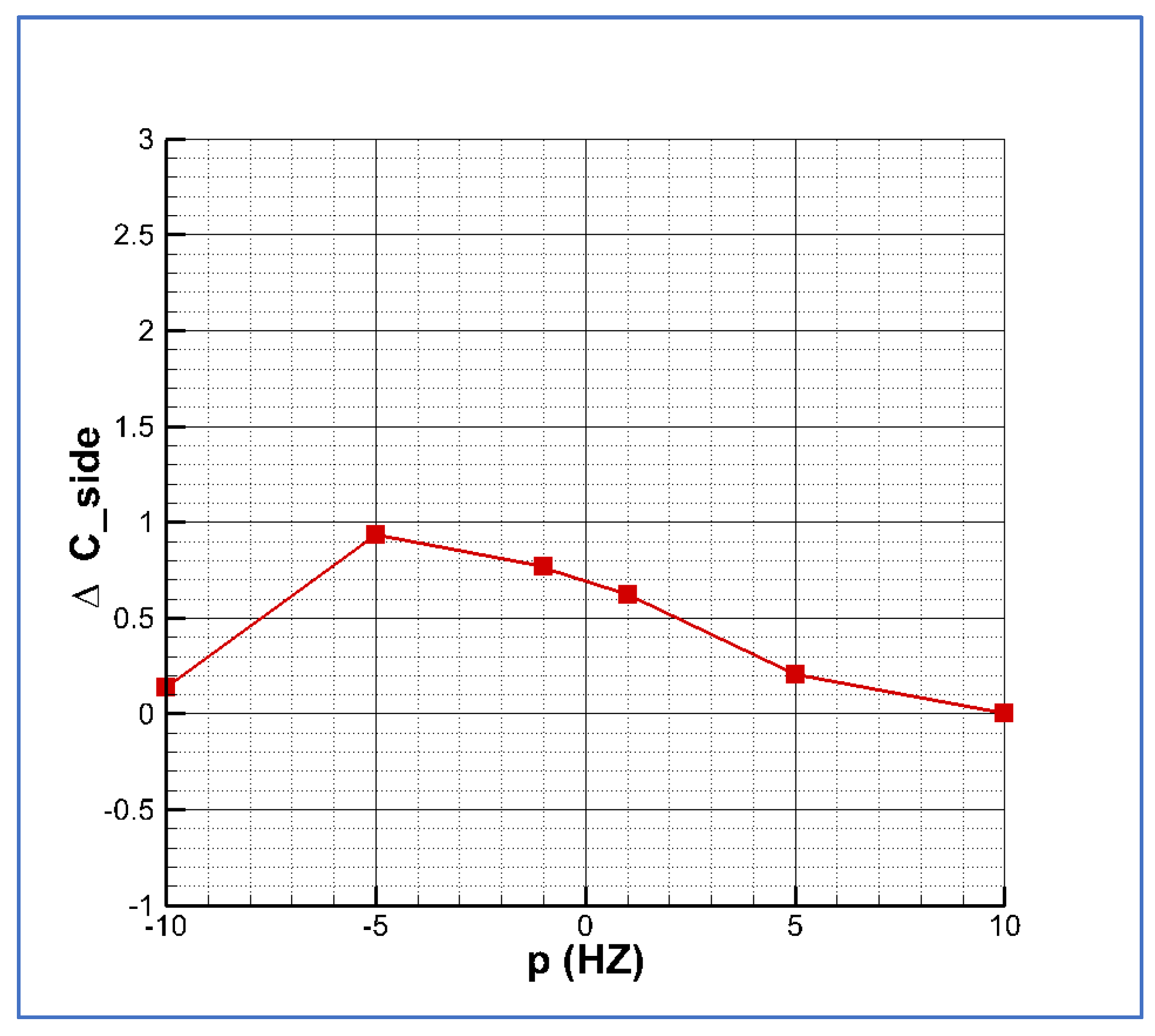
A good indicator of the strong asymmetry is shown in
Figure 14. The separation from the linear law built with the side force coefficient values (using in this case the average value for the two extreme solutions as reference) and crossing the point (0, 0) is plotted at the condition at an angle of attack α = 45 degrees.
The separation is larger at the negative roll rates than at the positive roll rates. Additionally, both values of this separation are positive. Therefore, there is a positive bias that indicates that rolling at lower velocities, approaching the limit of zero spin—either with negative spin or with positive spin—leads to a side force coefficient value of 0.70 approximately. This a quantification of the effect of this bias.
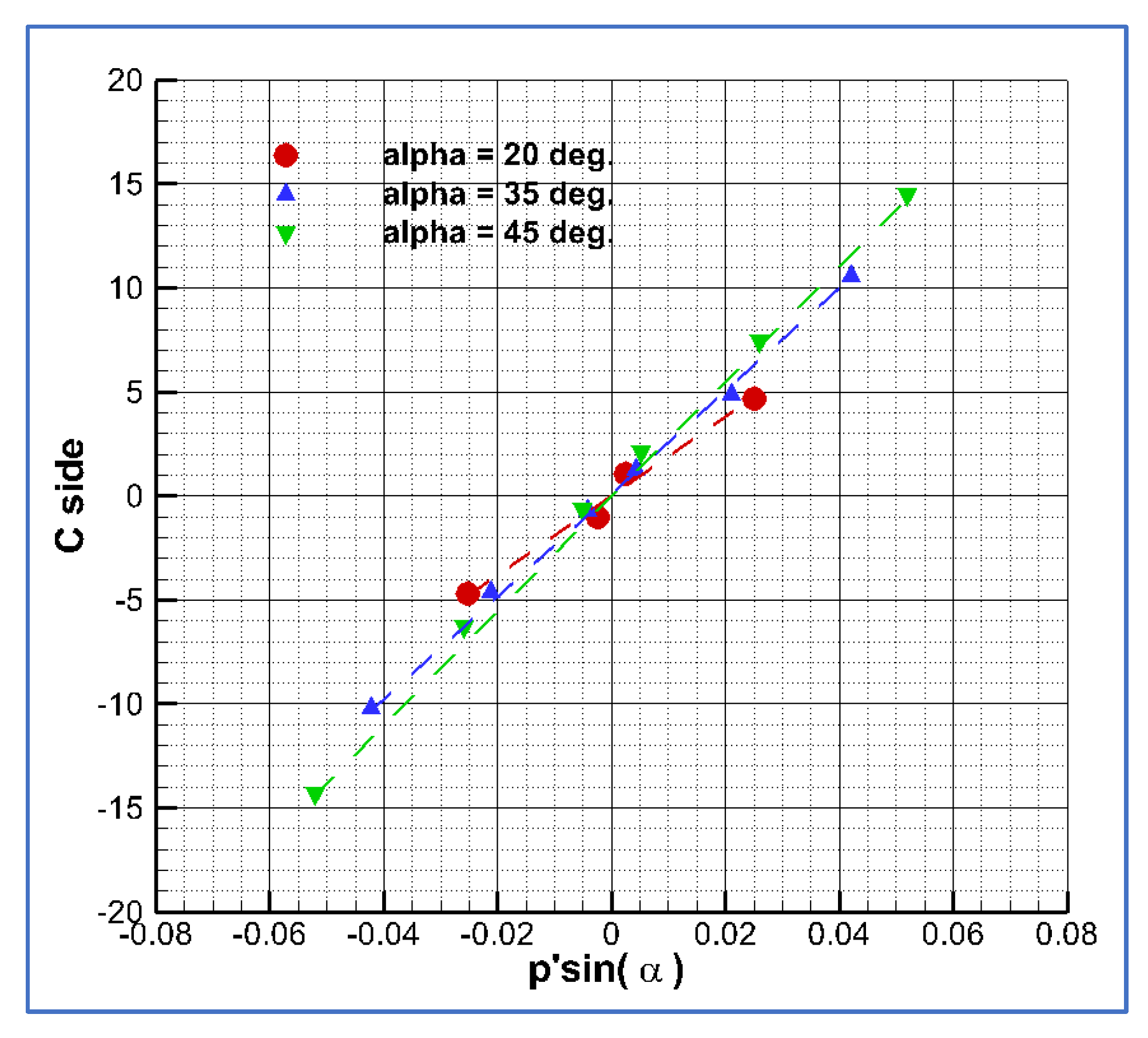
Nielsen [
2] defines as Magnus forces and moments those developing as a result of roll at angle of attack. Bhagwandin defines the Magnus side force as [
18]:
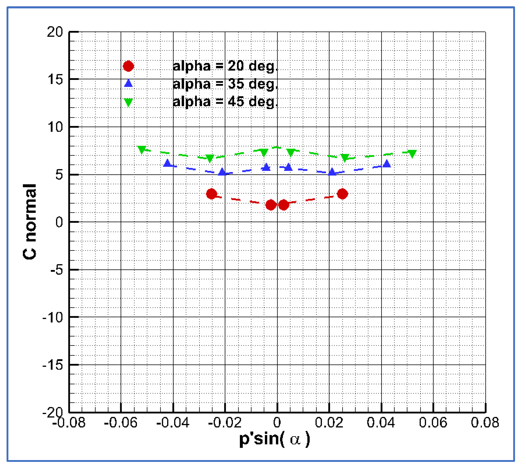
. A plot of the side force coefficient versus
is shown in
Figure 15. The lines are again drawn only for descriptive purposes. It was demonstrated in the previous figures that there is not a linear fit with the roll rate nor with the reduced roll rate or angle of attack. The slope of this curve provides a first approach to the Magnus derivative
. It can be seen that this derivative depends on the angle of attack, i.e.,
; therefore, is not constant, at least at high angles of attack, where the flow is non-symmetric at zero spin. The plot in
Figure 16 for the normal force coefficient shows that there is also a Magnus effect on the normal force and that the slope
is not constant. In this case, it is clear that there is not possible a quasi-linear fit approach. It depends on the roll rate and the angle of attack, i.e.,
.
For this case and looking at the solutions obtained at the different angles of attack and roll rates, the side and normal force coefficients could be defined as:
. The first term corresponds to the zero spin conditions, and for the larger angles of attack the side force coefficient is non-zero and also is roll dependent, being the term
the roll-averaged term. The last term can be explained as the result of the non-linear interaction effect due to a coupling of the rolling motion with the existing unsteady vortex flow pattern and high angles of attack. The intermediate term would be a “linear” Magnus effect. There is an in-plane Magnus (normal force coefficient) and an out-of-plane Magnus (side force coefficient). The values shown in
Figure 14 are a measurement of both the first and third terms defined above, i.e., a kind of measurement of
. A model with high-order terms at high angles of attack is described in ref. [
3], indicating the need for these terms under several conditions. The numerical solutions obtained show us that there may exist in these terms and are important.
A conclusion obtained after analyzing these curves is that, when calculating the Magnus effect due to rolling motion at large angles of attack, there are important non-linear effects that show that the force and moment coefficients cannot be approached by linear laws, and then, the stability derivatives have to be computed in a wide range of roll rates and angles of attack; these derivatives are to be variables and will depend at least on the spin velocity and on the angle of attack.
These calculations show that CFD can help build up a model of the forces and moments, which must take into account higher-order terms for the calculations of the stability derivatives.


