Simplified Maneuvering Strategies for Rendezvous in Near-Circular Earth Orbits

Abstract

The development of autonomous guidance control and navigation systems for spacecraft would greatly benefit applications such as debris removals or on-orbit servicing, where human intervention is not practical. Within this context, inspired by Autonomous Vision Approach Navigation and Target Identification (AVANTI) demonstration, this work presents new guidance algorithms for rendezvous and proximity operations missions. Analytical laws are adopted and preferred over numerical methods, and mean relative orbital elements are chosen as state variables. Application times, magnitudes and directions of impulsive controls are sought to minimize propellant consumption for the planar reconfiguration of the relative motion between a passive target spacecraft and an active chaser one. In addition, simple and effective algorithms to evaluate the benefit of combining in-plane and out-of-plane maneuvers are introduced to deal with 3D problems. The proposed new strategies focus on maneuvers with a dominant change in the relative mean longitude (rarely addressed in the literature), but they can also deal with transfers where other relative orbital elements exhibit the most significant variations. A comprehensive parametric analysis compares the proposed new strategies with those employed in AVANTI and with the global optimum, numerically found for each test case. Results are similar to the AVANTI solutions when variations of the relative eccentricity vector dominate. Instead, in scenarios requiring predominant changes in the relative mean longitude, the required $\Delta$V exhibits a 49.88% reduction (on average) when compared to the original methods. In all the test cases, the proposed solutions are within 3.5% of the global optimum in terms of $\Delta$V. The practical accuracy of the presented guidance algorithms is also tested with numerical integration of equations of motion with J2 perturbation.

1. Introduction

Mission success in current space proximity operations rely on complex instrumentation on board the satellites, intensive cooperation between the agents involved and the continuous contact with ground stations. Space agencies, as well as major research institutions worldwide, are more and more interested in increasing the technology readiness level of autonomous orbital rendezvous [1]. This technology would indeed be crucial for applications like debris removal, on-orbit servicing or distributed space systems. In particular, regarding the guidance layer, the spacecraft should be capable of computing, in real time, the reference trajectory and guarantee a near-optimal solution (minimum fuel or minimum time), without the intervention of ground operators. Consequently, the guidance task needs to be redefined to prioritize reliability, optimality, and computational efficiency. Several guidance schemes are present in the literature, differing in complexity of the dynamical model employed, the type of thrust provided by the engines, the state representation considered and the rationale used to compute the optimal solution (numerical or analytical methods) [2,3,4,5].

Anderson and Schaub [6] generalized the results presented in [7]; they formulated a linear programming framework to identify impulsive velocity changes required for prescribed orbital element adjustments between the deputy and chief spacecraft, with the objective of minimizing propellant consumption. However, their approach tends to permit more impulses than strictly necessary and does not determine the corresponding optimal application times. In their study [8], De Iuliis et al. identified fuel-optimal low-thrust profiles capable of executing formation reconfiguration, utilizing an improved version of the well-known Legendre pseudospectral method. On the other hand, Roscoe et al. [9] employed primer vector theory [10,11] to achieve impulsive orbital reconfiguration in the relative motion between two agents. Their method entails iteratively addressing the discrete fuel optimal guidance problem to match the optimal times of the continuous formulation. Both of these algorithms require substantial computational resources and well-informed initial guesses, making them not particularly suitable for autonomous guidance applications.

In recent years, there has been significant attention on successive convex optimization approaches, which can provide optimal trajectories for scenarios involving rendezvous and proximity operations, both reliable and accurate. This capability comes from the equivalence between the solution to the relaxed problem and the solution to the original nonlinear problem, demonstrated in [12]. Moreover, common constraints like keep-out-zones and thrust limitations can be easily incorporated into the optimization process [13]. At the same time, model predictive control algorithms have been proven to be a viable option for use in space applications, particularly in rendezvous, proximity operations, and docking missions [14,15]. These controllers can generate suboptimal trajectories in highly constrained environments, operating in a closed-loop fashion. Consequently, this approach reduces the impact of performance degradation resulting from sensor noise and maneuvers execution errors.

Convex programming and model predictive control methods, although potentially suitable for real-time applications due to their relative speed, necessitate the utilization of a dedicated software, such as primal–dual interior point algorithms, for solving the optimal control problems that stem from their formulations. A simpler and possibly equally (or almost equally) efficient alternative to these methods is the use of analytical algorithms. They are self-contained and enable the resolution of optimal guidance problems with a limited number of arithmetic calculations, without relying on external iterative algorithms and/or the availability of tentative solutions. For similar mission scenarios, it is therefore reasonable to assume that the computational times associated with these analytical approaches decrease compared to the latest numerical methods. In problems where high accuracy and robustness in the guidance solution are required (where the latest numerical procedures may be favored), such as rendezvous and proximity operations, analytical algorithms in general and the analytical schemes proposed in the present article remain valuable. Their solution can indeed be utilized as a ’warm start’ for more sophisticated numerical algorithms, as they provide a solid basis for informing the design of relative transfer trajectories and addressing the reconfiguration of the relative motion with additional fidelity.

Among analytical methods, Hablani et al. [16] employed the solution of the well-known Hill–Clohessy–Wiltshire equations [17] to develop guidance laws for approach to, departure from and circumnavigation of a target vehicle; despite the simplicity of the presented guidance algorithms, no optimization was treated. Bevilacqua and Romano [18] presented a guidance algorithm that exploits cooperation between a target and multiple chaser satellites for orbital rendezvous. All spacecrafts are supposed to be able to vary their wind cross-section in order to create a certain relative acceleration due to aerodynamic drag; the procedure is fully analytical, but it is not intended to deal with noncooperative rendezvous scenarios, in which the target could be an asteroid or a nonfunctional old satellite. Shuster et al. [19] described the reconfiguration of the relative motion by employing a parametrization derived from solving the Hill–Clohessy–Wiltshire equations. Through the application of primer vector theory, their methods systematically identify fuel optimal or suboptimal transfer trajectories to attain a specified set of relative orbital elements at the final time. Their work, while offering valuable insights into the guidance problem, solely concentrates on analyzing the resizing of passively safe ellipses or adjusting the phase angle of the deputy along a relative ellipse around the target. In [20], Gaias and D’Amico performed an exhaustive analysis of the relative orbital reconfiguration problem cast in relative orbital elements, and provided different analytical or semi-analytical algorithms comprising two or three impulses. Chernick and D’Amico [21] generalized one of the solutions presented in [20], considering the effects of the nonsphericity of the Earth or assuming elliptic reference orbits. In [20,21], the authors treated the planar and out-of-plane guidance problems separately, and the optimality of the algorithms, in terms of propellant consumption, is only referred to in specific cases, that is, when the relative eccentricity vector undergoes the most significant variation among the relative orbital elements.

This work extends the results of the work in [22] which is built upon the guidance algorithm described in [23] and implemented in the Autonomous Vision Approach Navigation and Target Identification (AVANTI) flight demonstration [24,25]. Mean relative orbital elements that are a nonlinear combination of mean absolute orbital elements of the two agents are used as state variables. New strategies are proposed to find application times, magnitudes and directions of impulsive controls in order to obtain assigned changes in relative orbital elements while minimizing propellant consumption.

Specific solutions are first obtained to solve for the planar reconfiguration of the relative motion between a target spacecraft and an active chaser one. The focus is on maneuvers with a dominant change in the relative mean longitude, referred in this paper as rephasing scenarios, which were typically not considered in previous works. However, generic maneuvers, i.e., when other mean relative orbital elements exhibit dominant changes, can also be treated. These solution are then extended to three-dimensional problems, evaluating the benefit of combining in-plane and out-of-plane maneuvers. Following this introduction, Section 2 offers the mathematical formulation of the problem for the reconfiguration of the relative motion. In Section 3, new closed-form maneuvering strategies are developed for both in-plane and 3D relative guidance. These strategies’ optimality and accuracy are subsequently verified through comprehensive numerical simulations in Section 4. Ultimately, Section 5 provides valuable insights into how the proposed algorithms can effectively address common mission constraints.

2. Problem Statement

An orbit is usually defined by the classical orbital elements (semi-major axis a, eccentricity e, argument of periapsis $\omega$, inclination i, right ascension of the ascending node $\mathsf{\Omega }$, mean anomaly M). In this paper, the absolute orbit of a spacecraft in the Earth Centered Inertial (ECI) reference frame is instead characterized by the following set of mean orbital elements:

$$\overrightarrow{\alpha }={(a, u, e_x, e_y, i, \mathsf{\Omega })}^T,$$

(1)

where $u=M+\omega$ represents the mean argument of latitude, and $e_x=ecos\omega$ and $e_y=esin\omega$ represent the components of the eccentricity vector (along and perpendicular to the line of nodes). In contrast to classical orbital elements, the set defined in Equation (1) is specifically designed to prevent singularities in near-circular reference orbits [26]. To describe the relative motion, we take the chief orbit as the reference and use the mean relative orbital elements (ROE) [26,27]. ROE are nonlinear combinations of the mean absolute orbital elements specified in Equation (1) for the chief and deputy satellites denoted by subscripts c and d, respectively:

$$\overrightarrow{\delta \alpha }=\left(\begin{array}{c}\delta a\\ \delta \lambda \\ \delta e_x\\ \delta e_y\\ \delta i_x\\ \delta i_y\end{array}\right)=\left(\begin{array}{c}\frac{a_d-a_c}{a_c}\\ u_d-u_c+({\mathsf{\Omega }}_d-{\mathsf{\Omega }}_c)cos{i}_c\\ e_{d}cos{\omega }_d-e_{c}cos{\omega }_c\\ e_{d}sin{\omega }_d-e_{c}sin{\omega }_c\\ i_d-i_c\\ ({\mathsf{\Omega }}_d-{\mathsf{\Omega }}_c)sin{i}_c\end{array}\right).$$

(2)

In particular, $\delta a$ is the relative semi-major axis, $\delta \lambda$ is the relative mean longitude, and $\overrightarrow{\delta e}={(\delta e_x, \delta e_y)}^T$ and $\overrightarrow{\delta i}={(\delta i_x, \delta i_y)}^T$ are the relative eccentricity and inclination vectors. It is useful to make reference to Hill’s coordinate frame, which is also known as an RTN (Radial–Tangential–Normal) coordinate frame. It is defined by unit vectors in the radial direction from the center of the Earth to the spacecraft (${\widehat{i}}_r$), in the tangential direction on the orbit plane (${\widehat{i}}_t$) and in the normal direction positive along the angular momentum vector (${\widehat{i}}_n$). Such moving reference frame is centered at the center of mass of the chief satellite, whose motion defines the reference orbit.

For near-circular reference orbits and when the relative orbit radius is small compared with the inertial reference orbit radius, $\delta a$ and $\delta \lambda$ represent the offsets in radial and tangential directions, respectively; $\overrightarrow{\delta e}$ describes amplitude and phase of in-plane motion (that is, on the plane of the chief’s orbit), whereas $\overrightarrow{\delta i}$ does the same for the out-of-plane motion [26,27]. In the absence of perturbations, the ROE remain constant over time, except for the relative mean longitude, whose time derivative can be approximated to first order as

$$\dot{\delta \lambda }=\frac{d\left(\delta \lambda \right)}{dt}=\frac{d\left(u_d\right)}{dt}-\frac{d\left(u_c\right)}{dt}=n_d-n_c\approx -\frac{3}{2}{n}_c\delta a,$$

(3)

where $n=\sqrt{\frac{\mu }{a^3}}$ is the mean motion and $\mu$ denotes the Earth’s gravitational parameter. Therefore, in a Keplerian two-body problem, the linearized relative motion of the deputy satellite with respect to the chief satellite in terms of the ROE is provided by

$$\overrightarrow{\delta \alpha }=\mathsf{\Phi }(u,u_0){\overrightarrow{\delta \alpha }}_0$$

(4)

with

$$\mathsf{\Phi }=\left(\begin{array}{cccccc}1& 0& 0& 0& 0& 0\\ -\frac{3}{2}(u-u_0)& 1& 0& 0& 0& 0\\ 0& 0& 1& 0& 0& 0\\ 0& 0& 0& 1& 0& 0\\ 0& 0& 0& 0& 1& 0\\ 0& 0& 0& 0& 0& 1\end{array}\right).$$

(5)

In Equation (4), we consider the reference mean argument of latitude u as the independent variable. The $6\times 6$ matrix in Equation (5), commonly referred to as the state transition matrix, maps the mean ROE at initial time $t_0$ (i.e., $u_0=u\left(t_0\right)$) to the corresponding values at generic time t (i.e., $u=u\left(t\right)$). This state transition matrix is utilized for the calculation of the optimal maneuvering schemes as described in Section 3. As confirmed by sources [23,28], the assumption of Keplerian motion is fully acceptable for our close proximity operations scenarios, given that the differential perturbations resulting from maneuvers have negligible effects. The consequences of neglecting these perturbations and potential reconfiguration errors are discussed in Section 4.

While the chief satellite is passive, the deputy is equipped with a propulsion system able to make corrections to the relative orbit. The Gauss variational equations, derived by Battin in [29], provide a mathematical framework for describing the rate of change in the osculating orbit elements of a spacecraft subject to a perturbing acceleration $\overrightarrow{\gamma }={({\gamma }_r, {\gamma }_t, {\gamma }_n)}^T$, expressed in the RTN reference frame. These Gauss variational equations can be readily applied to the orbital elements introduced in Equation (1). Assuming a near-circular orbit (i.e., $e\approx 0$) and considering only the perturbed response of the mean argument of latitude u, we can obtain

$$\frac{d{\overrightarrow{\alpha }}_{osc}}{dt}=\frac{1}{na}B\left({\overrightarrow{\alpha }}_{osc}\right)\overrightarrow{\gamma }$$

(6)

with

$$B\left({\overrightarrow{\alpha }}_{osc}\right)=\left(\begin{array}{ccc}0& 2a& 0\\ -2& 0& -\frac{sinu}{tani}\\ sinu& 2cosu& 0\\ -cosu& 2sinu& 0\\ 0& 0& cosu\\ 0& 0& \frac{sinu}{sini}\end{array}\right),$$

(7)

where subscript osc denotes the osculating orbital elements. When impulsive acceleration is applied at a generic time denoted as $t_j$, the integration of Equation (6) over the impulse establishes the relation between the instantaneous change in velocity $\overrightarrow{\delta v_j}={(\delta v_r, \delta v_t, \delta v_n)}_j^T$ in the RTN frame and the subsequent instantaneous changes in the spacecraft osculating orbital elements ${\overrightarrow{\Delta \alpha }}_{osc,j}$ [30,31]. We remark that notation $\Delta \left(·\right)$ stands for the arithmetic difference of the orbital elements after and before the maneuver, and the velocity step is such that $\overrightarrow{\delta v_j}={\int }_{t_j^{-}}^{t_j^{+}}\overrightarrow{\gamma }dt$. The results above can be extended to our proximity operation scenarios using the Gauss variational equations to express the rate of change in the osculating ROE as

$$\frac{d{\overrightarrow{\delta \alpha }}_{osc}}{dt}=\frac{1}{n_c{a}_c}\frac{\partial {\overrightarrow{\delta \alpha }}_{osc}}{\partial {\overrightarrow{\alpha }}_{c,osc}}B\left({\overrightarrow{\alpha }}_{c,osc}\right)\overrightarrow{{\gamma }_c}+\frac{1}{n_d{a}_d}\frac{\partial {\overrightarrow{\delta \alpha }}_{osc}}{\partial {\overrightarrow{\alpha }}_{d,osc}}B\left({\overrightarrow{\alpha }}_{d,osc}\right)R({\overrightarrow{\alpha }}_{c,osc},{\overrightarrow{\alpha }}_{d,osc})\overrightarrow{{\gamma }_d},$$

(8)

where $R({\overrightarrow{\alpha }}_{c,osc},{\overrightarrow{\alpha }}_{d,osc})$ is the rotation matrix from the chief’s RTN frame to the deputy’s RTN frame. Due to our linearization assumption, the effects of maneuvers on the osculating and the mean ROE can be considered identical [21,28], and recalling that the chief is passive, the integration of Equation (8) over the course of the maneuver applied at generic time $t_j$ yields

$${\overrightarrow{\Delta \delta \alpha }}_j\approx \frac{1}{n_c{a}_c}{\mathsf{\Psi }}_j\left({\overrightarrow{\alpha }}_c\right){\overrightarrow{\delta v}}_j=\frac{1}{n_c{a}_c}\frac{\partial \overrightarrow{\delta \alpha }}{\partial {\overrightarrow{\alpha }}_d}{B}_j\left({\overrightarrow{\alpha }}_c\right){\overrightarrow{\delta v}}_j$$

(9)

with

$${\mathsf{\Psi }}_j=\left(\begin{array}{ccc}0& 2& 0\\ -2& 0& 0\\ sin{u}_j& 2cos{u}_j& 0\\ -cos{u}_j& 2sin{u}_j& 0\\ 0& 0& cos{u}_j\\ 0& 0& sin{u}_j\end{array}\right).$$

(10)

In this work, we deal with a fixed-time impulsive reconfiguration problem: given the initial mean ROE at $t_0$ (i.e., the initial time or $u_0$), we want to obtain a final mean ROE vector at $t_F$ (i.e., a specified final time or $u_F$) with impulsive control actions while minimizing propellant consumption. The mathematical formulation of the reconfiguration problem can be written as

$$n_c{a}_c({\overrightarrow{\delta \alpha }}_F-\mathsf{\Phi }(u_F,u_0){\overrightarrow{\delta \alpha }}_0)=\sum _{j=1}^N\mathsf{\Phi }(u_F,u_j){\mathsf{\Psi }}_j{\overrightarrow{\delta v}}_j,$$

(11)

where the application of N maneuvers results in the achievement of the aimed mean ROE variation on the left-hand side of Equation (11). For instance, if $N=2$, Equation (11) can be decomposed into

$$\begin{array}{cc}\hfill \overrightarrow{\delta {\alpha }_1}& =\mathsf{\Phi }(u_1,u_0)\overrightarrow{\delta {\alpha }_0}+\frac{1}{na}{\mathsf{\Psi }}_1\overrightarrow{\delta v_1},\hfill \\ \hfill \overrightarrow{\delta {\alpha }_2}& =\mathsf{\Phi }(u_2,u_1)\overrightarrow{\delta {\alpha }_1}+\frac{1}{na}{\mathsf{\Psi }}_2\overrightarrow{\delta v_2}=\mathsf{\Phi }(u_2,u_0)\overrightarrow{\delta {\alpha }_0}+\frac{1}{na}\mathsf{\Phi }(u_2,u_1){\mathsf{\Psi }}_1\overrightarrow{\delta v_1}+\frac{1}{na}{\mathsf{\Psi }}_2\overrightarrow{\delta v_2},\hfill \\ \hfill \overrightarrow{\delta {\alpha }_F}& =\mathsf{\Phi }(u_F,u_2)\overrightarrow{\delta {\alpha }_2}.\hfill \end{array}$$

(12)

Finally, the square of total velocity variation is the cost function to be minimized:

$$J={\left(\sum _{i=1}^N\sqrt{\delta v_{ir}^2+\delta v_{it}^2+\delta v_{in}^2}\right)}^2.$$

(13)

The function in Equation (13) is an index of propellant expenditure and it is constrained by the dynamics introduced in Equation (11).

3. Reconfiguration Strategies

The reconfiguration problem is characterized by six aimed mean ROE variations (four for the planar case), and every impulse has four parameters (three for the planar case): the corresponding times of application (or $u_i$) and the three components (two for the planar case). Each algorithm proposed in this paper imposes some constraints on the impulses and reduces the number of parameters in order to obtain an algebraic system of equations. Due to the assumption of Keplerian dynamics, the in-plane and out-of-plane dynamics are decoupled.

Table 1. Summary of Presented Procedures.

Scheme Identifier	Dimensionality	Number of Impulses	Maneuver Type
1	2D	3	RT-RT-RT
2	3D	4	RT-RT-RT-N
3	3D	3	RTN-RTN-RTN
4	3D	3	RTN-RTN-RTN

summarizes the strategies introduced hereafter, with their main characteristics. The maneuver type in the fourth column identifies the components of applied $\overrightarrow{\delta v}$ (R-radial, T-tangential, N-normal). We note that Scheme 3 and 4 have the same maneuver types as three 3D impulses, but differ in the position of the impulses along the orbit, as shown later in this section. All the procedures are generic in the sense that no restrictions or constraints on aimed mean ROE variations have to be imposed to find a solution. Scheme 1 is a three-impulse planar reconfiguration. Scheme 2 contributes an additional impulse to the planar solution to perform the out-of-plane maneuver for a four-impulse 3D reconfiguration. Schemes 3 and 4 also solve the three-dimensional case, but use only three impulses: Scheme 3 places the impulses at the same positions as in the planar case (Scheme 1); Scheme 4 instead moves one of the impulses of the planar solution to the position of the out-of-plane maneuver in Scheme 2.

The algorithm employed in the AVANTI demonstration accomplishes the in-plane reconfiguration through the application of three tangential impulses. In contrast, Scheme 1 revisits the in-plane reconfiguration problem by utilizing three impulses while introducing radial components. This inclusion of radial impulses indeed contributes to the improvement of fixed-time phasing maneuvers, which are often necessary in real-world scenarios. From Equation (11), the in-plane reconfiguration problem is described by

$$n_c{a}_c\left(\begin{array}{c}\Delta \delta a\\ \Delta \delta \lambda \\ \Delta \delta e_x\\ \Delta \delta e_y\end{array}\right)=\sum _{j=1}^3\left(\begin{array}{cc}0& 2\\ -2& -3(u_f-u_j)\\ sin\left(u_j\right)& 2cos\left(u_j\right)\\ -cos\left(u_j\right)& 2sin\left(u_j\right)\end{array}\right)\left(\begin{array}{c}\delta v_{rj}\\ \delta v_{tj}\end{array}\right).$$

(14)

Scheme 1 obtains the solution in two steps: the first one reduces the number of free parameters to four with suitable assumptions and provides the starting solution for the second one. This paper focuses on strategies that can deal with predominant variation in the relative mean longitude. As shown by Equation (3), the longer the time between impulses, the lower the change in relative semi-major axis needed to modify $\delta \lambda$. For this reason, the first impulse is fixed at the beginning of the reconfiguration, that is, $u_1=u_0$, and a radial component is added to the tangential component at the first impulse, whereas the remaining two maneuvers remain purely tangential. Their positions (i.e., $u_2$ and $u_3$) are discretized over a sufficient dense grid, with $u_1<u_2<u_3$ and $u_F-\pi \le u_3\le u_F$. The choice of grid density is illustrated and justified in Section 4.1. We note that the allowable values of $u_3$ are chosen to exploit, as much as possible, the time available for the reconfiguration of relative motion (i.e., $u_F-u_0$). With $u_1$, $u_2$ and $u_3$ specified and $\delta v_{r2}=\delta v_{r3}=0$, Equation (14) becomes a linear four-equation system with four unknowns $\delta v_{r1}$, $\delta v_{t1}$, $\delta v_{t2}$, and $\delta v_{t3}$, which is readily solved: $\delta v_{t3}$ is first determined and used to obtain the other unknowns. We have

$$\delta v_{t3}=\frac{(\overline{\Delta \delta \lambda }+1.5u_F\overline{\Delta \delta a}-2\overline{\Delta \delta e_y})D_1+[2sin\left(u_2\right)-1.5u_F-0.5q](\overline{\Delta \delta e_x}-\overline{\Delta \delta a})}{D_1[-4sin\left(u_3\right)+p]+D_2[-4sin\left(u_2\right)+q]-3u_F[cos\left(u_3\right)-cos\left(u_2\right)]},$$

(15)

$$\delta v_{r1}=\frac{[2D_{2}sin\left(u_2\right)+2D_{1}sin\left(u_3\right)]\delta v_{t3}+sin\left(u_2\right)(\overline{\Delta \delta e_x}-\overline{\Delta \delta a})-D_1\overline{\Delta \delta e_y}}{D_1},$$

(16)

$$\delta v_{t1}=\left(-\frac{D_2}{D_1}-1\right)\delta v_{t3}+0.5\overline{\Delta \delta a}-\frac{\overline{\Delta \delta e_x}-\overline{\Delta \delta a}}{2D_1},$$

(17)

$$\delta v_{t2}=\frac{\overline{\Delta \delta e_x}-\overline{\Delta \delta a}+2D_2\delta v_{t3}}{2D_1},$$

(18)

with $D_1=-1+cos{u}_2$, $D_2=1-cos{u}_3$, $q=-3(u_F-u_2)$ and $p=-3(u_F-u_3)$. Different solutions are evaluated for the selected ($u_2,u_3$) combinations, and the minimum one in terms of cost index in Equation (13) is retained.

This solution may have suboptimal performances because it excludes the radial components for the second and third impulses. The second step improves the solution by recognizing that the optimization of selected index cost J is a convex problem with respect to $\overrightarrow{\delta v}$ components. The best parametric solution can therefore be refined analytically, solving the well-known Karush–Kuhn–Tucker (KKT) system of equations:

$$\left[\begin{array}{cc}\left[H^{*}\right]& {\left[G\right]}^T\\ \left[G\right]& 0\end{array}\right]\left(\begin{array}{c}\overrightarrow{\Delta x}\\ \overrightarrow{\lambda }\end{array}\right)=\left(\begin{array}{c}-\overrightarrow{g}\\ -\overrightarrow{c}\end{array}\right),$$

(19)

where $\overrightarrow{\Delta x}$ is a column vector composed of the sought corrections of the in-plane components of the three impulses (i.e., the variables of the KKT system of equations):

$$\overrightarrow{x}={(x_1,x_2,x_3,x_4,x_5,x_6)}^T={(\delta v_{t1},\delta v_{t2},\delta v_{t3},\delta v_{r1},\delta v_{r2},\delta v_{r3})}^T.$$

(20)

Column vector $\overrightarrow{g}={\frac{\partial J}{\partial \overrightarrow{x}}}^T$ represents the gradient of cost function J with respect to $\overrightarrow{x}$:

$$\begin{array}{c}\hfill g_1=\frac{\delta v_1+\delta v_2+\delta v_3}{\delta v_1}2x_1,\end{array}$$

(21)

$$\begin{array}{c}\hfill g_2=\frac{\delta v_1+\delta v_2+\delta v_3}{\delta v_2}2x_2,\end{array}$$

(22)

$$\begin{array}{c}\hfill g_3=\frac{\delta v_1+\delta v_2+\delta v_3}{\delta v_3}2x_3,\end{array}$$

(23)

$$\begin{array}{c}\hfill g_4=\frac{\delta v_1+\delta v_2+\delta v_3}{\delta v_1}2x_4,\end{array}$$

(24)

$$\begin{array}{c}\hfill g_5=\frac{\delta v_1+\delta v_2+\delta v_3}{\delta v_2}2x_5,\end{array}$$

(25)

$$\begin{array}{c}\hfill g_6=\frac{\delta v_1+\delta v_2+\delta v_3}{\delta v_3}2x_6,\end{array}$$

(26)

with $\delta v_j=\sqrt{\delta v_{tj}^2+\delta v_{rj}^2}$ being the magnitudes of the impulses. The Hessian

$$\left[H\right]=\frac{{\displaystyle \partial {\left(\frac{\partial J}{\partial \overrightarrow{x}}\right)}^T}}{{\displaystyle \partial \overrightarrow{x}}}$$

(27)

is a $6\times 6$ symmetric matrix, $\overrightarrow{c}$ is a column vector defined by the constraints in Equation (14), and $\left[G\right]=\frac{\partial \overrightarrow{c}}{\partial \overrightarrow{x}}$ is the Jacobian of constraints

$$\left[G\right]=\left[\begin{array}{cccccc}2& 2& 2& 0& 0& 0\\ -3(u_F-u_1)& -3(u_F-u_2)& -3(u_F-u_3)& -2& -2& -2\\ 2cos{u}_1& 2cos{u}_2& 2cos{u}_3& sin{u}_1& sin{u}_2& sin{u}_3\\ 2sin{u}_1& 2sin{u}_2& 2sin{u}_3& -cos{u}_1& -cos{u}_2& -cos{u}_3\end{array}\right].$$

(28)

Equation (19) is solved with the values of Step 1 solution and provides corrections $\overrightarrow{\Delta x}$ to determine the refined solution. We should note that the application times of the maneuvers do not change. Details on the corresponding theory can be found in [32].

Scheme 1 considers the planar case, whereas the other strategies deal with the three-dimensional problem. Scheme 2 in Table 1 exploits the uncoupled in-plane/out-of-plane dynamics and considers a separate impulse to change the relative plane. One additional normal impulse is necessary and sufficient to reconfigure the relative inclination vector. The out-of-plane maneuver of the general 3D reconfiguration problem is described by

$$\sum _j\delta v_{nj}cos\left(u_{nj}\right)=n{a}_c\Delta \delta i_x,$$

(29)

$$\sum _j\delta v_{nj}sin\left(u_{ni}\right)=n{a}_c\Delta \delta i_y,$$

(30)

with $j=1,\dots ,N^{\prime }$ that denotes the number of normal impulses. Considering only one impulse, from Equations (29) and (30) with $N^{\prime }=1$, we have

$$\delta v_n=n{a}_c\sqrt{{(\Delta \delta i_x)}^2+{(\Delta \delta i_y)}^2},$$

(31)

and the corresponding mean argument of latitude is given by

$$u_{ns}=arctan\left(\frac{\Delta \delta i_y}{\Delta \delta i_x}\right)+k\pi ,$$

(32)

where $k\in {\mathbb{N}}_0$ and is such that $u_{ns}<u_F$. Finally, the cost index of Scheme 2, which has a separate impulse for the plane change, can be evaluated as

$$J_{sep}={\left(\sum _{j=1}^3\sqrt{\delta v_{rj}^2+\delta v_{tj}^2}+\left|\delta v_n\right|\right)}^2.$$

(33)

Scheme 3 in Table 1 performs in-plane and out-of-plane maneuvers simultaneously in contrast to Scheme 2. The planar and out-of-plane reconfiguration problems have decoupled dynamics and can be solved in sequence. Scheme 3 starts from the unrefined planar solution of Scheme 1 and then introduces additional out-of-plane impulse components at two of the in-plane reconfiguration maneuvers to obtain three-dimensional transfer. The out-of-plane maneuvers ($n1$, $n2$) occur at the locations of two impulses of the unrefined planar solution; one can set $u_{n1}<u_{n2}$, and the available options are ($u_{n1}=u_1,u_{n2}=u_2$), ($u_{n1}=u_1,u_{n2}=u_3$), and ($u_{n1}=u_2,u_{n2}=u_3$). The magnitudes of velocity changes are then easily found by inverting Equations (29) and (30), with two normal impulses ($N^{\prime }=2$):

$$\delta v_{n1}=-\frac{1}{dfcos\left(u_{n1}\right)}(\overline{\Delta \delta i_y}-tan\left(u_{n2}\right)\overline{\Delta \delta i_x}),$$

(34)

$$\delta v_{n2}=\frac{1}{dfcos\left(u_{n2}\right)}(\overline{\Delta \delta i_y}-tan\left(u_{n1}\right)\overline{\Delta \delta i_x}),$$

(35)

with $df=tan\left(u_{n2}\right)-tan\left(u_{n1}\right)$. Based on different combinations of $u_{n1}$ and $u_{n2}$, three solutions are obtained, and the one associated with the lowest cost index defined in Equation (13) is retained. Once again, this solution is then improved by solving the system in Equation (19), extended to three-dimensional cases. The mean arguments of latitude of the impulses keep the same value of the unrefined solution, and the vector of unknowns (the components of the three $\overrightarrow{\delta v}$) is augmented to

$$\overrightarrow{x}={(x_1,x_2,x_3,x_4,x_5,x_6,x_7,x_8,x_9)}^T={(\delta v_{t1},\delta v_{t2},\delta v_{t3},\delta v_{r1},\delta v_{r2},\delta v_{r3},\delta v_{n1},\delta v_{n2},\delta v_{n3})}^T.$$

(36)

Scheme 4 in Table 1 again combines planar and nonplanar maneuvers, but, in contrast to Scheme 3, it does not maintain the impulses at the positions of the corresponding planar problem. One of the planar impulses is instead placed at the position defined by Equation (32), that is, the mean argument of latitude of the cross-track impulse $u_{ns}$ of Scheme 2. More specifically, quantity

$$d_{m,n}=\left|u_m-\left[arctan\left(\frac{\Delta \delta i_y}{\Delta \delta i_x}\right)+k_n\pi \right]\right|$$

(37)

is introduced to evaluate which impulse ($m=1,2,3$) has the minimum angular distance from the position of the cross-track impulse. Indeed, as shown below in Section 4.2, when the position of the planar impulse is close to $u_{ns}$, the combination of the in-plane and out-of-plane maneuvers can provide relevant propellant savings, relative to the separate approach. Equations (14) are then easily inverted to obtain $\overrightarrow{\delta v}$ in-plane components corresponding to the new triplet of mean arguments of latitude. Then, the system in Equation (19), again adapted to a three-dimensional case, is solved in order to decrease the cost index of Equation (13).

Practically, we can compare the cost index introduced in Equation (33) with the cost index of the combined approaches of Schemes 3 and 4 and choose the most convenient strategy. Indeed, all the procedures described above are analytical, and few more calculations do not compromise the performance of the code in terms of computational time.

4. Results

The solutions of the proposed schemes are derived for Keplerian orbits and a linearized dynamic. In this section, a numerical validation of the proposed strategies in terms of optimality and accuracy in a nonlinear dynamical model with J2 perturbation are presented. A numerical propagator, which takes into account J2 perturbation, is employed to calculate Cartesian positions and velocities of both the deputy and chief satellites within the Earth-centered reference frame. 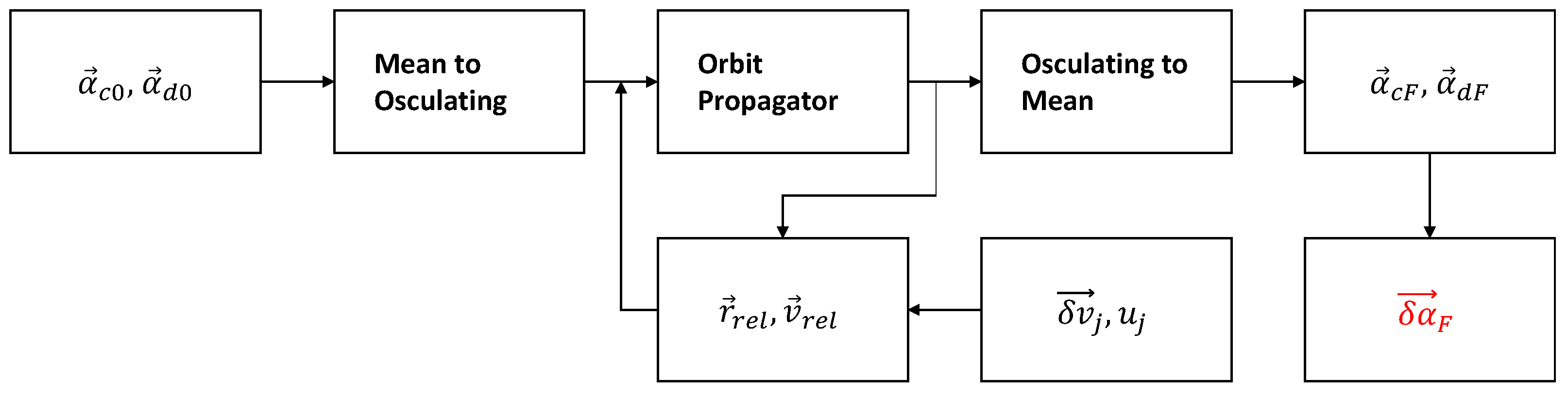As shown in Figure 1, the orbit propagator is initialized with the osculating orbital elements of both satellites, derived from the corresponding mean orbital elements and using the linear mapping developed by Schaub and Junkins [33]. Impulsive maneuvers, calculated using the algorithms presented in this paper, are introduced as discontinuities in the relative velocity of the deputy satellite within the RTN reference frame. At the end of the predetermined time interval available for reconfiguration, the osculating orbital elements of both satellites are converted back to their corresponding mean values, and the final mean relative orbital elements are extracted. After the simulation, the achieved and desired mean relative orbital elements are compared to assess the accuracy of the closed-form maneuvering schemes.

In test Case 1, in-plane reconfiguration is analyzed using the solution of Scheme 1 in Table 1. Results are compared with the global optimum and with the strategy adopted in the AVANTI demonstration [23]. The global optimum is obtained using Matlab function fmincon, with $4N$ parameters ($3N$ for the planar case) that correspond to the application times and the components of number N of impulses. The numeric optimization procedure is initialized with the unrefined solution of Scheme 1 and it utilizes sequential quadratic programming as the nonlinear optimizer. Two parametric analyses are also performed to infer the goodness of the solution of Scheme 1 with respect to different aimed reconfiguration parameters (i.e., variations in mean relative orbital elements). In test Case 2, the three-dimensional problem is considered and different values of inclination vector change are used to assess and compare the performance of Schemes 2, 3 and 4.

4.1. Test Case 1—In-Plane Control

The chief orbit is a near-circular low Earth orbit and is described by the following absolute mean orbital elements:

$${[a,e,i,\mathsf{\Omega },\omega ,M]}_c=[R_E+750 \mathrm{km}, 0.001, {80}^{\circ }, 0^{\circ }, 0^{\circ }, 0^{\circ }],$$

(38)

where $R_E$ is the Earth radius. Mean relative orbital elements at the initial and final time, as well as the mean relative orbital elements total variations, are

$$a_c{(\delta a,\delta \lambda ,\delta e_x,\delta e_y)}_0=(50, -\mathrm{10,000}, 230, -50) \mathrm{m},$$

(39)

$$a_c{(\delta a,\delta \lambda ,\delta e_x,\delta e_y)}_F=(0, -5000, 150, 0) \mathrm{m},$$

(40)

$$a_c(\Delta \delta a,\Delta \delta \lambda ,\Delta \delta e_x,\Delta \delta e_y)=(-50,5942.5,-80,50) \mathrm{m}.$$

(41)

The predominant variation regards the relative mean longitude, and the final value of the mean argument of latitude is set equal to $u_F=4\pi$, that is, a fast re-phasing scenario with two revolutions around the Earth. We note that time t and the reference mean argument of latitude are related by $u=nt$ and the duration of the mission is approximately $3.33$ h. This representative case is used to assess the discretization grid density introduced in Scheme 1. The size of the grid equals the product of the number of samples considered for each variable: if the number of variables is large and/or the discretization step is small, the time required to obtain a solution with a grid-based search could be prohibitive. On the other hand, an excessively large discretization step may lead to an unsatisfactory solution in terms of a certain figure of merit that in our case is the cost index defined in Equation (13). The problem presented at the beginning of this section is resolved by considering three different discretization grids, similarly to what was performed in [34]. Specifically, all the three grids are equally spaced, but the discretization steps are set equal to ${20}^{\circ },1^{\circ }$ and ${0.05}^{\circ }$ for the first, second and third grid, respectively.

The best grid points in the fourth column of

Table 2. Grid Search Algorithm.

Step, ${}^{\circ }$	Time, s	Samples	Best Points, m/s	Optimized Value, m/s	Deviation, %
20	0.01	350	0.3106	0.3075	0.9992
1	0.03	130139	0.3105	0.3075	0.9799
0.05	2.53	51850799	0.3105	0.3075	0.9799

indicate the square root of the cost index of the unrefined solution for Scheme 1 (i.e., without solving the KKT system of equations). Instead, the optimized value in the fifth column is the square root of the optimal cost index obtained using Matlab function fmincon, initialized with the corresponding unrefined solution and with sequential quadratic programming as the nonlinear optimizer. The computational time of the finest grid is approximately two orders of magnitude greater than that of the grid with a step size of $1^{\circ }$, even though the performance in terms of optimality is nearly identical. On the other hand, choosing a step size of $1^{\circ }$ allows for achieving a cost index that is closer to the optimal value compared to that of the grid with a step size of ${20}^{\circ }$, while still maintaining the computational time within fully acceptable values (hundredths of a second). It is therefore reasonable to use a discretization step of $1^{\circ }$ for $u_2$ and $u_3$ in Scheme 1.

Table 3. Test Case 1 Solutions.

-	Scheme 1	AVANTI	Numerical
$u_1,\mathrm{rad}$	0	2.5830	0
$u_2,\mathrm{rad}$	8.8550	5.7246	9.4540
$u_3,\mathrm{rad}$	12.5573	8.8662	12.5664
$\delta v_{1T},\mathrm{m}/\mathrm{s}$	−0.1654	−0.2964	−0.1645
$\delta v_{2T},\mathrm{m}/\mathrm{s}$	0.0084	−0.0379	0.0079
$\delta v_{3T},\mathrm{m}/\mathrm{s}$	0.1308	0.3080	0.1304
$\delta v_{1R},\mathrm{m}/\mathrm{s}$	−0.0264	0	−0.0296
$\delta v_{2R},\mathrm{m}/\mathrm{s}$	−0.0012	0	−0.0002
$\delta v_{3R},\mathrm{m}/\mathrm{s}$	−0.0204	0	−0.0235
$\sqrt{J},\mathrm{m}/\mathrm{s}$	0.3083	0.6422	0.3075
%	0.2716	108.8497	-

compares the results of Scheme 1, AVANTI demonstration strategy and global optimum. Scheme 1 is very close to the global optimum and clearly outperforms the strategy implemented for AVANTI demonstration, which was specifically designed to better work when the shape of the relative orbit (i.e., relative eccentricity vector) is the predominant change [23], and is therefore not suited for this test case. The initial and final times of reconfiguration (i.e., 0 and $3.33$ h) are the optimal application times of the first and last impulses, respectively, as shown by the numerical solution. It is well known that the best strategy to change the mean longitude is to move the spacecraft to a phasing orbit with a different period (that is, by changing a, and, as a consequence, $\delta a$); once again, the longer the time spent in drift, the lower the relative major-axis change to achieve the same longitude. Scheme 1 follows this strategy here, with almost tangential first and last impulses to modify $\delta a$, which are close to the initial and final time, respectively. A small intermediate impulse is added for minor adjustments after $2.34$ h from the beginning of the mission.

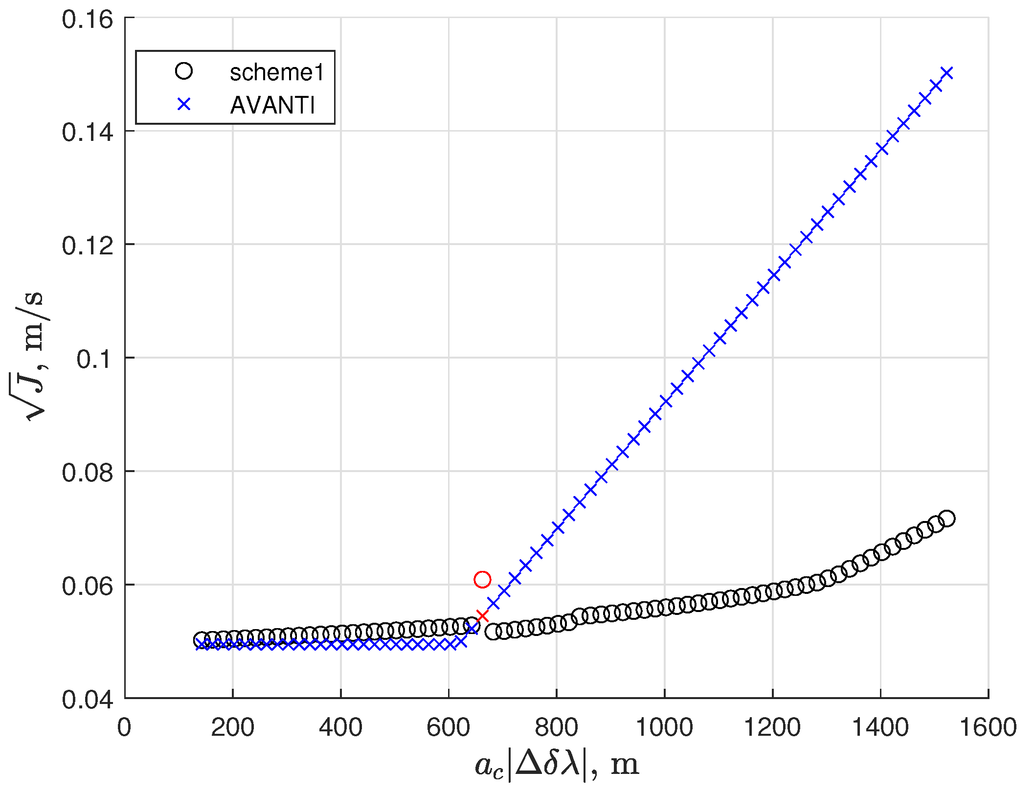
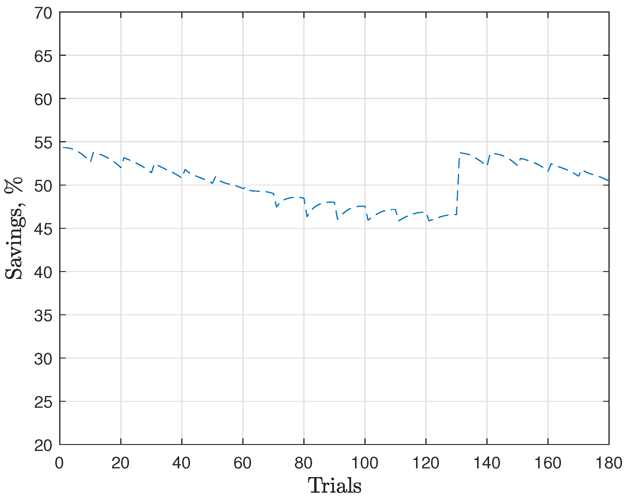
Even though Scheme 1 is designed for rephasing scenarios, it is intrinsically flexible and it can almost reach the minimum propellant consumption even when the relative mean longitude is not the parameter that varies the most. This feature is shown in Figure 2, where the square roots of the cost indexes of Scheme 1 (black circles) and of AVANTI code (blue markers) are plotted for increasing $a_c\left|\Delta \delta \lambda \right|$, while keeping the other changes in orbital parameters constant. For the small changes (less than approximately 643 m), AVANTI is slightly better than the Scheme 1 solution, which becomes more convenient for larger values. It should be noted that, at the point where $a_c\left|\Delta \delta \lambda \right|=662.5\mathrm{m}$ (as indicated by the red symbols in Figure 2), Scheme 1 exhibits a noticeable decline in performance compared to other cases. This decline stems from a possible drawback of the search grid algorithm utilized in Scheme 1, which struggles to accurately identify the optimal positions of the impulses (i.e., $u_2$ and $u_3$), resulting in the attainment of only a local minimum [34]. Nevertheless, it is noteworthy that the percentage difference between the square roots of the cost indexes of Scheme 1 and AVANTI algorithm in that point amounts to just $11.78\%$.

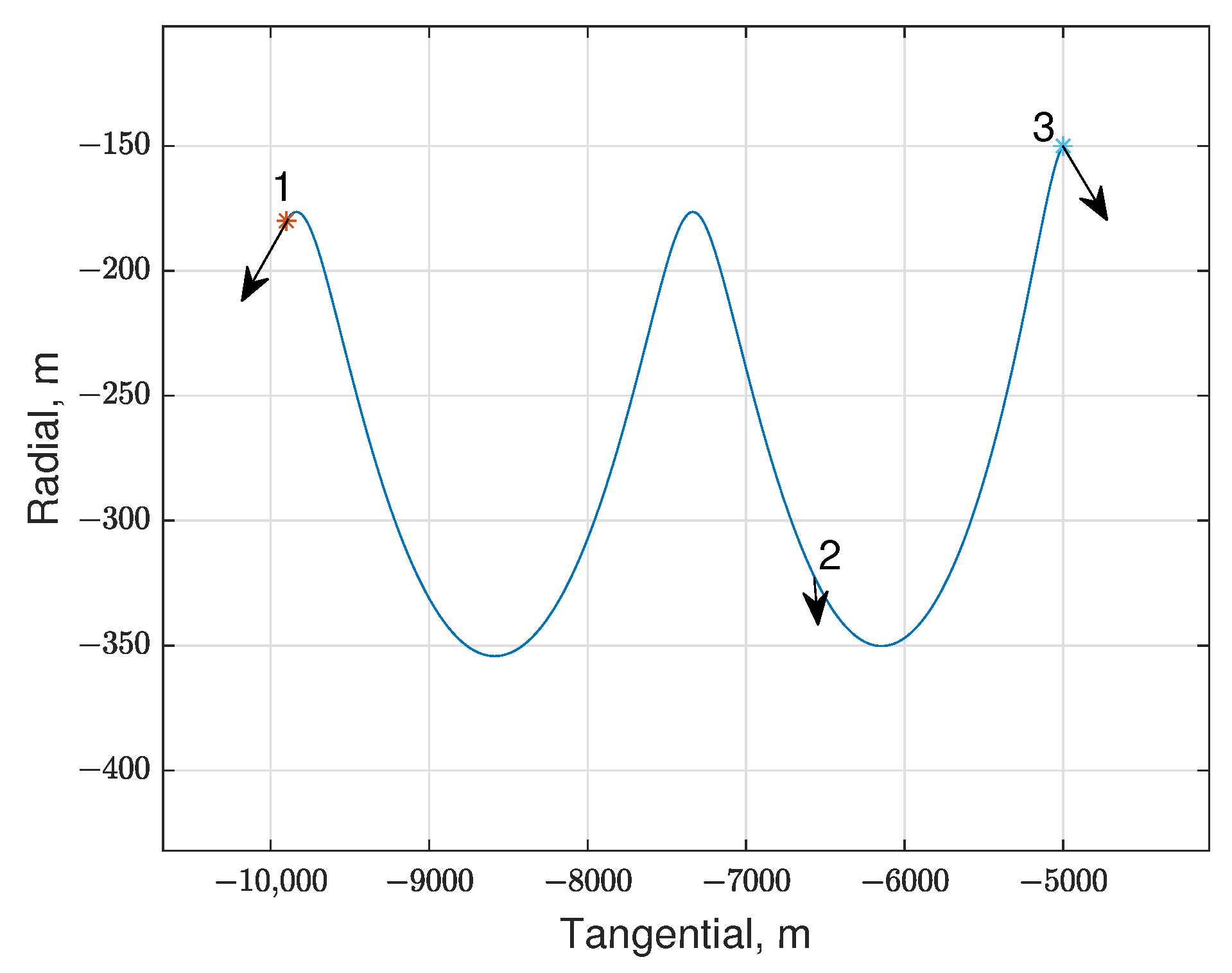
For Scheme 1, Figure 3 shows the relative 2D trajectory of the deputy in the Hill’s coordinate frame centered on the chief spacecraft. The linear mapping provided in D’Amico [26] has been used to convert ROE into Hill’s coordinates. Red and light blue asterisks denote the initial and final relative position, respectively, whereas Points 1, 2 and 3 indicate where the impulses (arrows) are applied.

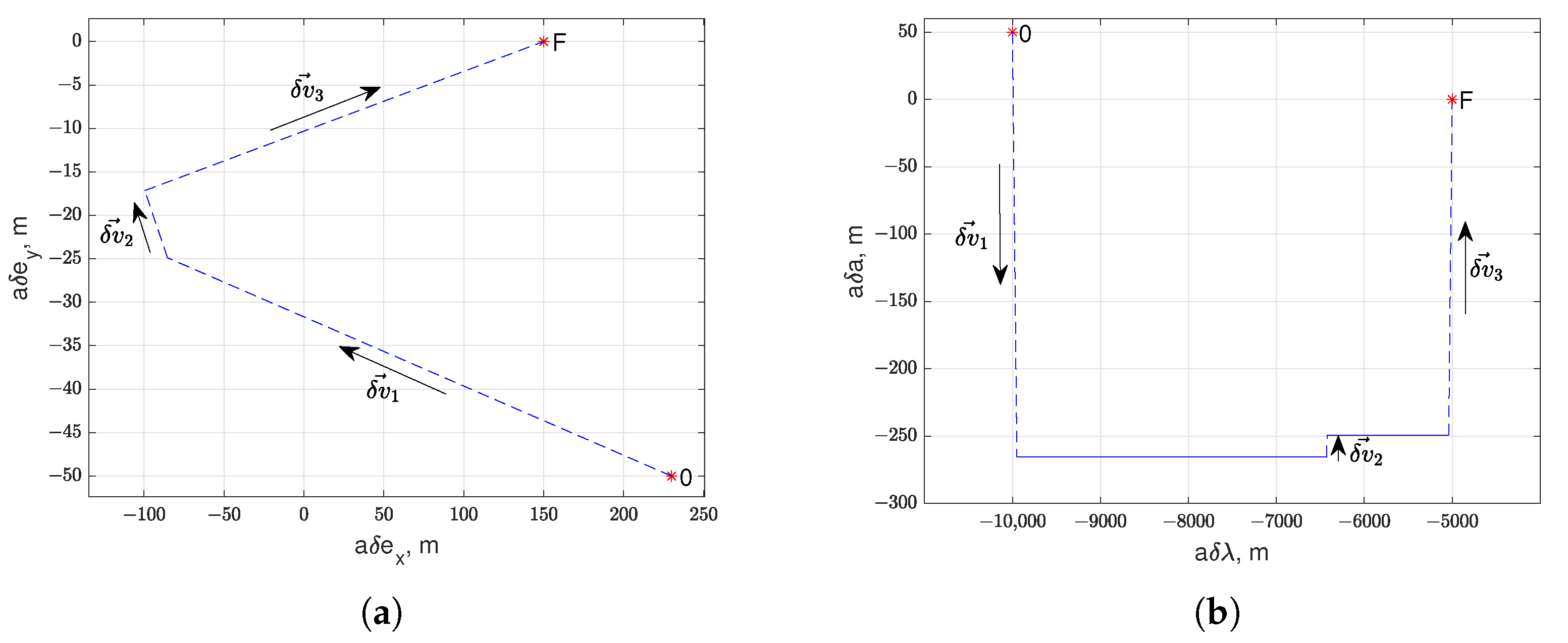
Figure 4a,b depict the transfer in the relative eccentricity vector plane and in the relative semi-major axis/relative mean longitude plane, respectively. Red asterisks with 0 and F indicate initial and final values of the corresponding mean relative orbital elements. The dotted lines represent the instantaneous changes in the mean relative orbital elements due to the impulses, whereas the solid lines denote the evolution of the mean relative orbital elements due to the natural dynamics (only the relative mean longitude varies linearly with time).

Table 4. Accuracy of the reconfiguration for Scheme 1.

	Mean Relative Orbital Elements, m
	${\mathit{a}}_{\mathit{c}}\mathit{\delta }\mathit{a}$	${\mathit{a}}_{\mathit{c}}\mathit{\delta }\mathit{\lambda }$	${\mathit{a}}_{\mathit{c}}\mathit{\delta }{\mathit{e}}_{\mathit{x}}$	${\mathit{a}}_{\mathit{c}}\mathit{\delta }{\mathit{e}}_{\mathit{y}}$
Desired	0	−5000	150	0
Achieved	−0.2386	−5000.5059	150.1075	−2.7300

displays the results of the simulation outlined in Figure 1, when Scheme 1 is employed to address the reconfiguration problem introduced at the beginning of this section. Errors in the achieved mean relative orbital elements, arising from the omission of perturbations and linearization assumptions, are less than 3 m.

Parametric analysis including 1690 reconfiguration problems is performed to infer how different variations of mean relative orbital elements affect the performance of Scheme 1 with respect to the AVANTI algorithm. All changes of the mean ROE take different values and specifically $a_c\Delta \delta a$ and $a_c\Delta \delta e_x$ vary from $-100 \mathrm{m}$ to $80 \mathrm{m}$ with a step of $15 \mathrm{m}$, $a_c\Delta \delta e_y$ from $10 \mathrm{m}$ to $100 \mathrm{m}$ with a step of $10 \mathrm{m}$, whereas the relative mean longitude change is such that the aimed final value is $a_c\delta {\lambda }_F=-5000 \mathrm{m}$, and the initial value is $a_c\delta {\lambda }_0=-10,000 \mathrm{m}$. Figure 5 shows the percentage propellant saving of Scheme 1 with respect to the AVANTI algorithm, that is, on average, of 49.88%.

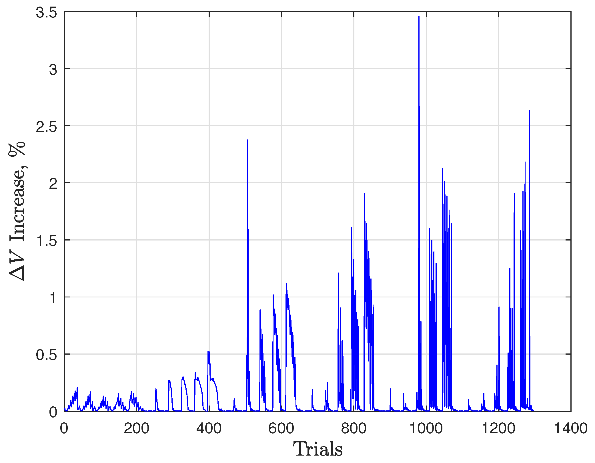
A second parametric analysis is carried out to better understand how different variations of mean relative orbital elements as well as different time windows could influence the performance of Scheme 1 in terms of optimality. In this case, 1296 reconfiguration problems are considered: $a_c\Delta \delta a$ and $a_c\Delta \delta e_x$ vary from $-40 \mathrm{m}$ to $+60 \mathrm{m}$ with a step of $20 \mathrm{m}$, $a_c\Delta \delta e_y$ from $0 \mathrm{m}$ to $50 \mathrm{m}$ with a step of $10 \mathrm{m}$, and the predominant change in relative mean longitude is such that $a_c\delta {\lambda }_F=-3000 \mathrm{m}$ and $a_c\delta {\lambda }_0=-\mathrm{10,000} \mathrm{m}$. The final mean argument of latitude $u_F$ is an additional parameter that ranges from $4\pi$ to $5\pi$. Figure 6 reports the percentage $\Delta V$ growth with respect to the global optimum, always lower than 3.5%.

On average, the time to solve each reconfiguration problem is $0.05$ seconds on a PC based on Intel (R) Core(TM) i7-10750H CPU @ 2.60 GHz 2.59 GHz using a nonoptimized Matlab code, fully suitable for the mentioned autonomous guidance applications. For comparison, the solution with fmincon and the AVANTI solution as a tentative guess is typycally 10–20 times slower.

4.2. Test Case 2—3D Control

For this test case, the same reference orbit of test Case 1 is used, described by Equation (38). The in-plane mean ROE aimed variations are the ones from Equation (41) and the corresponding solution using Scheme 1 is discussed in Table 3. Schemes 2 and 3 in Table 1 are then applied for $M=179$ of relative inclination vector variations, all of the same magnitude:

$$a_c{\left|\left(\overrightarrow{\Delta \delta i}\right)\right|}_j=a_c\sqrt{{(\Delta \delta i_x)}_j^2+{(\Delta \delta i_y)}_j^2}=90 \mathrm{m},$$

(42)

with $j=1,\dots ,M$ and phases described by Equation (32) ranging from $1^{\circ }$ to ${179}^{\circ }$.

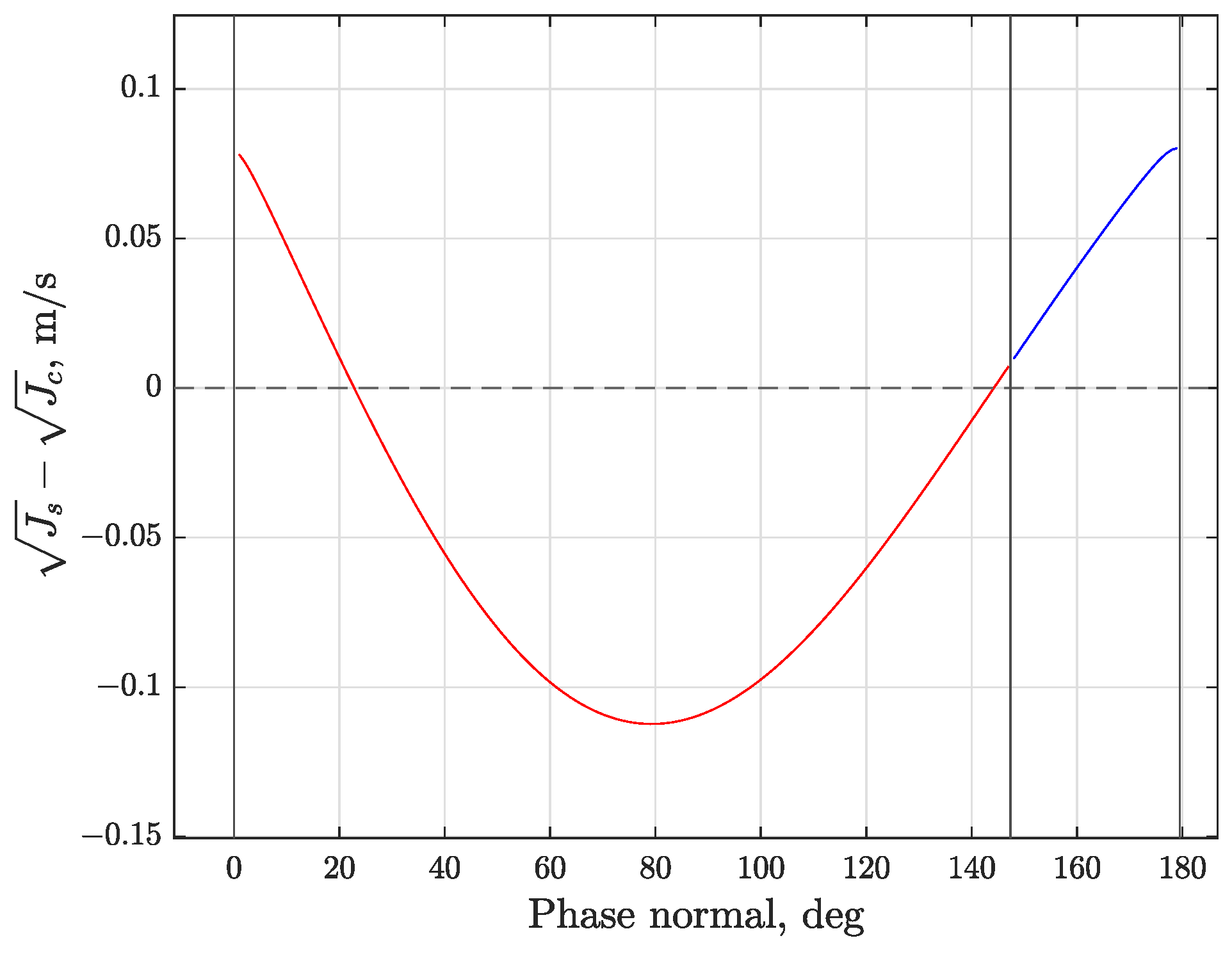
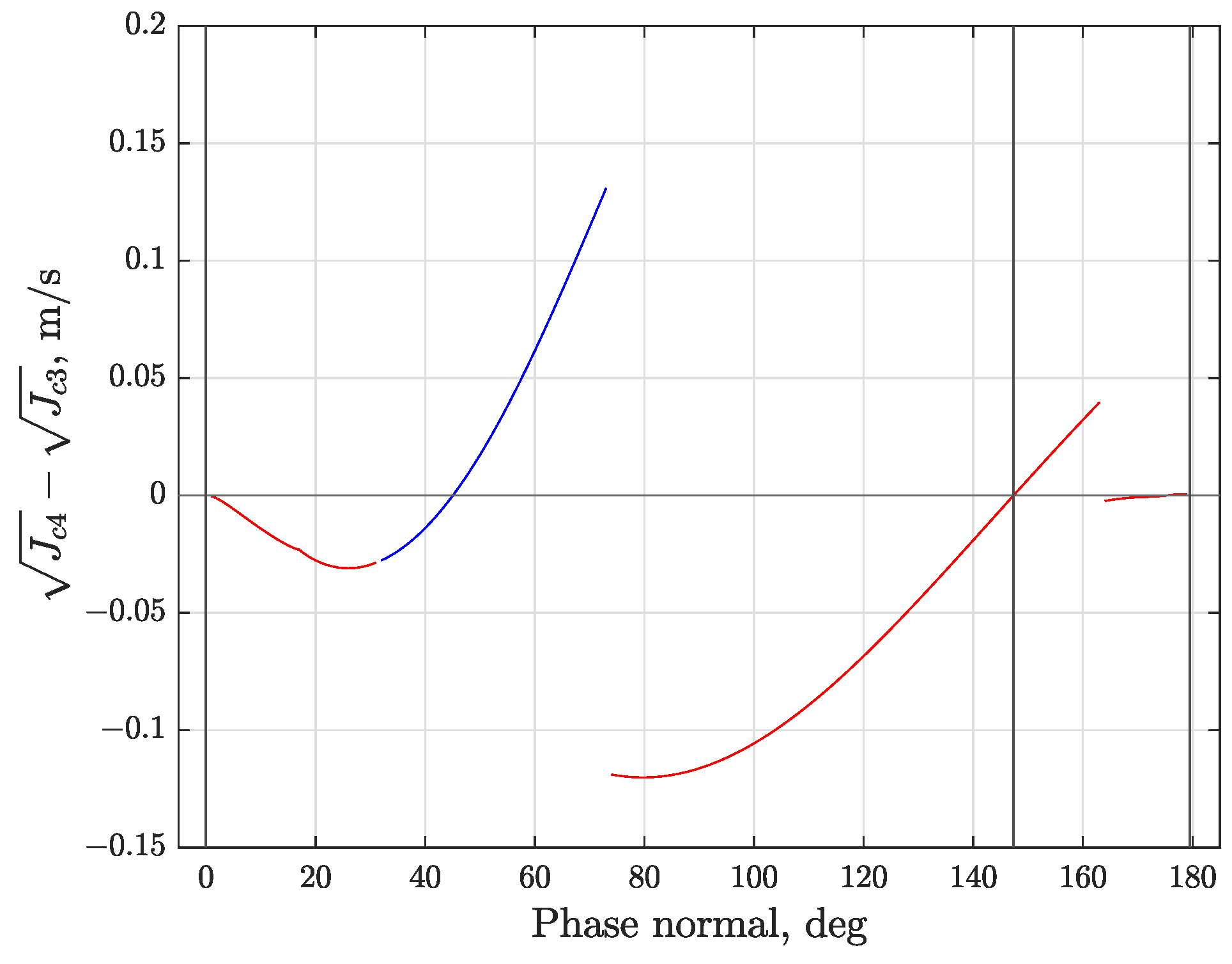
In Figure 7, the difference in the square root of the cost index of Scheme 2 minus the square root of the cost index of Scheme 3 is plotted versus the phase of relative inclination vector variations. The vertical black lines indicate the angular positions, wrapped to the interval $0^{\circ }$–${180}^{\circ }$ of the planar impulses. The plot color distinguishes solutions where the out-of-plane components of $\overrightarrow{\delta v}$ are added at the first and second planar impulses (red) from cases where the addition is at the second and third ones (blue). It is evident that the out-of-plane components of the impulses are more favorable at the positions that surround the phase of the required inclination change. When the plotted difference is positive, Scheme 3 outperforms Scheme 2, i.e., the combination of in-plane and out-of-plane maneuvers leads to propellant savings with respect to the separate approach. For the out-of-plane reconfiguration only, minimum $\Delta V$ is obtained with one or more impulses applied at the mean arguments of latitude $u_{ns}$, defined in Equation (32) [23]. When 3D reconfiguration is considered and the phase $u_{ns}$ is sufficiently close to the positions of the planar impulses selected by Scheme 3, the combination of the impulses is definitely convenient. In these cases (here, for phases close to either $0^{\circ }$ or ${180}^{\circ }$), it is advantageous to slightly shift the normal impulses in time (i.e., different $u_{ns}$) and to combine them with the planar impulses due to vector combination properties.

The same analysis is used to compare the performances of Schemes 2 and 4.

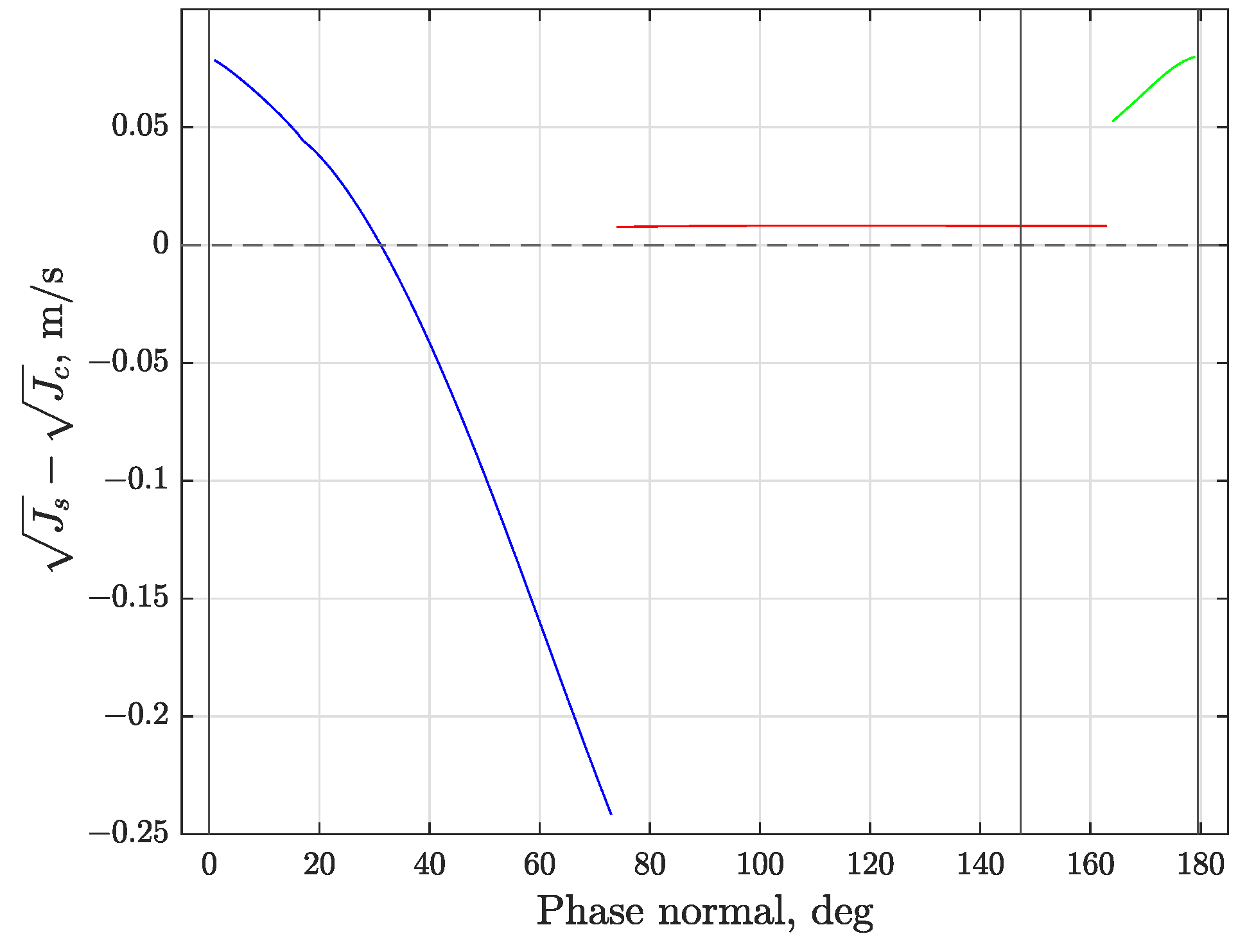
In Figure 8, the difference in the square root of the cost index of Scheme 2 minus the square root of the cost index associated with Scheme 4 is plotted with respect to the phase of the relative inclination vector variation. Once again, the vertical black lines represent the values of the mean argument of latitude of the planar impulses (wrapped to $0^{\circ }$–${180}^{\circ }$), and the line color identifies which planar impulse is moved to the mean arguments of latitude of the cross-track maneuver: blue for the first, red for the second, and green for the third. When the plotted difference is positive, the combination of planar and out-of-plane maneuvers is beneficial. Figure 8 reveals that it is convenient to disrupt the optimal planar solution and to move one of the planar impulses when the corresponding mean argument of latitude is sufficiently close to $u_{ns}$ due, again, to vector combination. In similarity to Scheme 3, it is favorable to move the impulse which is closer to the required phase of the relative inclination vector variation. We note that when the second planar impulse is moved (red line), since its magnitude is small (compared to the magnitudes of first and third impulses), the vector combination yields only a modest reduction in the performance index.

Figure 9 plots the square root of the cost index associated with Scheme 4 minus the square root of the cost index associated with Scheme 3. The blue line identifies the cases in which both Schemes 3 and 4 do not outperform the separate strategy, contrary to the red lines, for which at least one of the combined strategies is beneficial. For this particular reconfiguration problem, Scheme 4 is more convenient than Scheme 3 when combination is useful, excluding two small ranges of the phase that vary from ${148}^{\circ }$ to ${163}^{\circ }$ and from ${176}^{\circ }$ to ${179}^{\circ }$. We note that when $u_{ns}$ is very close to the mean arguments of latitude of the planar impulses, the plotted difference approaches zero, meaning that almost the same cost reduction can be obtained with both Schemes 3 and 4.

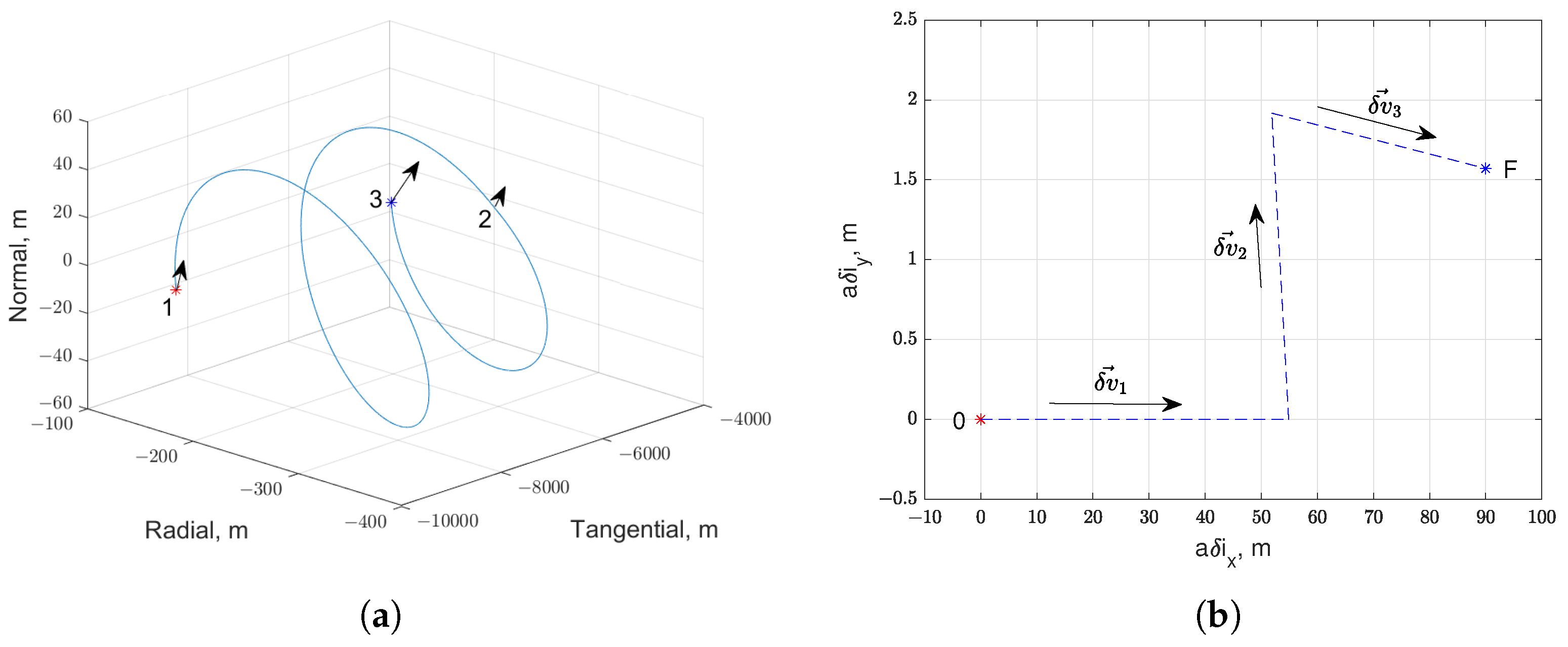
Figure 10a shows the relative trajectory of the deputy in the Hill’s coordinate frame centered on the chief spacecraft, referring to Scheme 3. Among the M reconfiguration problems of test Case 2, the phase of the total variation in the relative inclination vector is fixed to $u_{ns}=1^{\circ }$. Red and blue asterisks denote the initial and final relative position, respectively, whereas Points 1, 2 and 3 indicate where the impulses are applied. Figure 10b illustrates the same transfer just described, but depicted in the relative inclination vector plane. The three dotted lines represent the instantaneous changes in the relative inclination vector components due to the three impulses. As expected, most of the out-of-plane reconfiguration is performed with the first and the last impulse, whose mean arguments of latitude are close to $u_{ns}$, and only a small normal component is used with the second impulse (note the different scales of the axes).

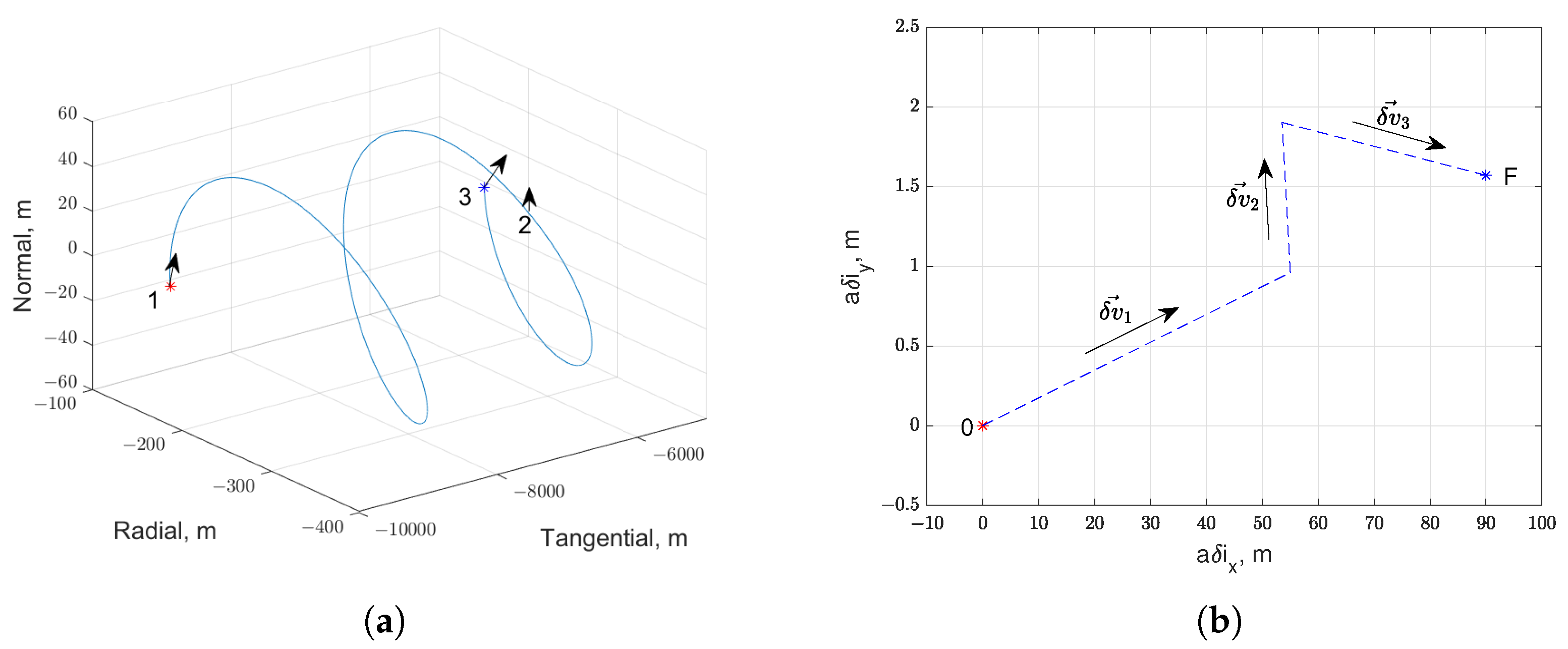
Figure 11a shows the solution with Scheme 4 for the same maneuver ($u_{ns}=1^{\circ }$). The initial and final relative positions are identified by the red and blue asterisks, respectively, and Points 1, 2, and 3 are where the impulses are applied. The three dotted lines in Figure 11b connect the three different relative inclination vectors, achieved by the impulsive maneuvers. Similar to the previous results for Scheme 3, Scheme 4 concentrates most of the out-of-plane change in correspondence to the first and the last impulses, as their positions are close to $u_{ns}$.

As in the case of planar reconfiguration,

Table 5. Accuracy of the reconfiguration for Schemes 2, 3 and 4.

		Mean Relative Orbital Elements, m
Algorithm	Metric	${\mathit{a}}_{\mathit{c}}\mathit{\delta }\mathit{a}$	${\mathit{a}}_{\mathit{c}}\mathit{\delta }\mathit{\lambda }$	${\mathit{a}}_{\mathit{c}}\mathit{\delta }{\mathit{e}}_{\mathit{x}}$	${\mathit{a}}_{\mathit{c}}\mathit{\delta }{\mathit{e}}_{\mathit{y}}$	${\mathit{a}}_{\mathit{c}}\mathit{\delta }{\mathit{i}}_{\mathit{x}}$	${\mathit{a}}_{\mathit{c}}\mathit{\delta }{\mathit{i}}_{\mathit{y}}$
Scheme 2	Desired	0	−5000	150	0	89.9863	1.5707
	Achieved	−0.2774	−5001.5310	150.1351	−2.7309	89.9618	0.2859
Scheme 3	Desired	0	−5000	150	0	89.9863	1.5707
	Achieved	−0.2781	−5001.0765	150.1301	−2.7313	89.9647	−0.7769
Scheme 4	Desired	0	−5000	150	0	89.9863	1.5707
	Achieved	−0.2897	−4992.6705	150.6405	2.7705	89.9661	−1.7231

displays the accuracy of the proposed algorithms when, among the M reconfiguration problems of test Case 2, the phase of the total variation in the relative inclination vector is fixed to $u_{ns}=1^{\circ }$. It is noteworthy that all the algorithms successfully attain the desired reconfiguration with a high degree of accuracy, as evidenced by errors in the mean relative orbital elements of less than 8 m.

5. Trajectory Constraints

In proximity operations and rendezvous scenarios, mission requirements may impose constraints on either the state variables or control inputs. To demonstrate the ability of the proposed algorithms in managing these constraints, we utilize the linear mapping discussed in Section 4, recalled here for comprehensive understanding. Cartesian components $y_1, y_2, y_3$ of position vector $\overrightarrow{y}={(y_1, y_2, y_3)}^T$ in the RTN frame are expressed at the generic mean argument of latitude u as

$$\overrightarrow{y}\left(u\right)=M\left(u\right)a\overrightarrow{\delta \alpha }\left(u\right)=M\left(u\right)\mathsf{\Phi }(u,u_0)a\overrightarrow{\delta \alpha }\left(u_0\right)+\frac{1}{n}\sum _{j}M\left(u\right)\mathsf{\Phi }(u,u_j)\mathsf{\Psi }\left(u_j\right){\overrightarrow{\delta v}}_j$$

(43)

by using matrix

$$M\left(u\right)=\left[\begin{array}{cccccc}1& 0& -cosu& -sinu& 0& 0\\ 0& 1& 2sinu& -2cosu& 0& 0\\ 0& 0& 0& 0& sinu& -cosu\end{array}\right].$$

(44)

By employing Equation (43), the constraints are straightforwardly expressed as functions of the unknowns within the problem, specifically the components of the impulses. Detailed discussion of constraint handling is beyond the scope of the present article, but two simple examples are here discussed for a planar problem with

$${\overrightarrow{\delta \alpha }}_0=(0, -200, 230, -70) \mathrm{m},$$

(45)

$${\overrightarrow{\delta \alpha }}_F=(0, -190, 100, 0) \mathrm{m}.$$

(46)

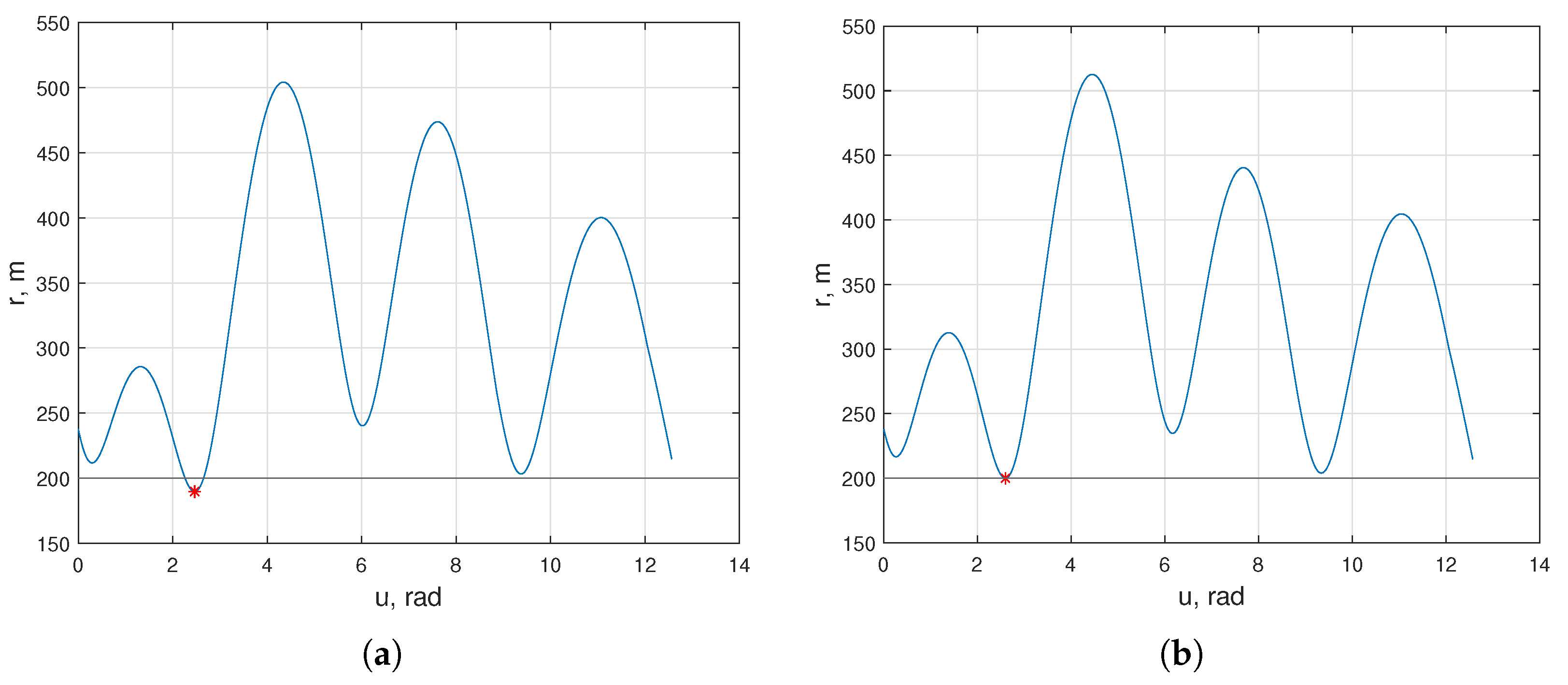
The reference orbit is the same defined in Equation (38) and $u_F=4\pi$. First, a specific way-point is introduced by forcing the deputy to be at y = 0 in the RTN frame (i.e., above or below the chief) at a specified $u=\overline{u}$ in the planar reconfiguration example. The constrained solution can be obtained by adding constraint $y_2\left(\overline{u}\right)=0$ during the refinement of Scheme 1 solution. The KKT system of Equation (19) is thus rewritten accordingly and solved to obtain the required $\Delta V$ components.

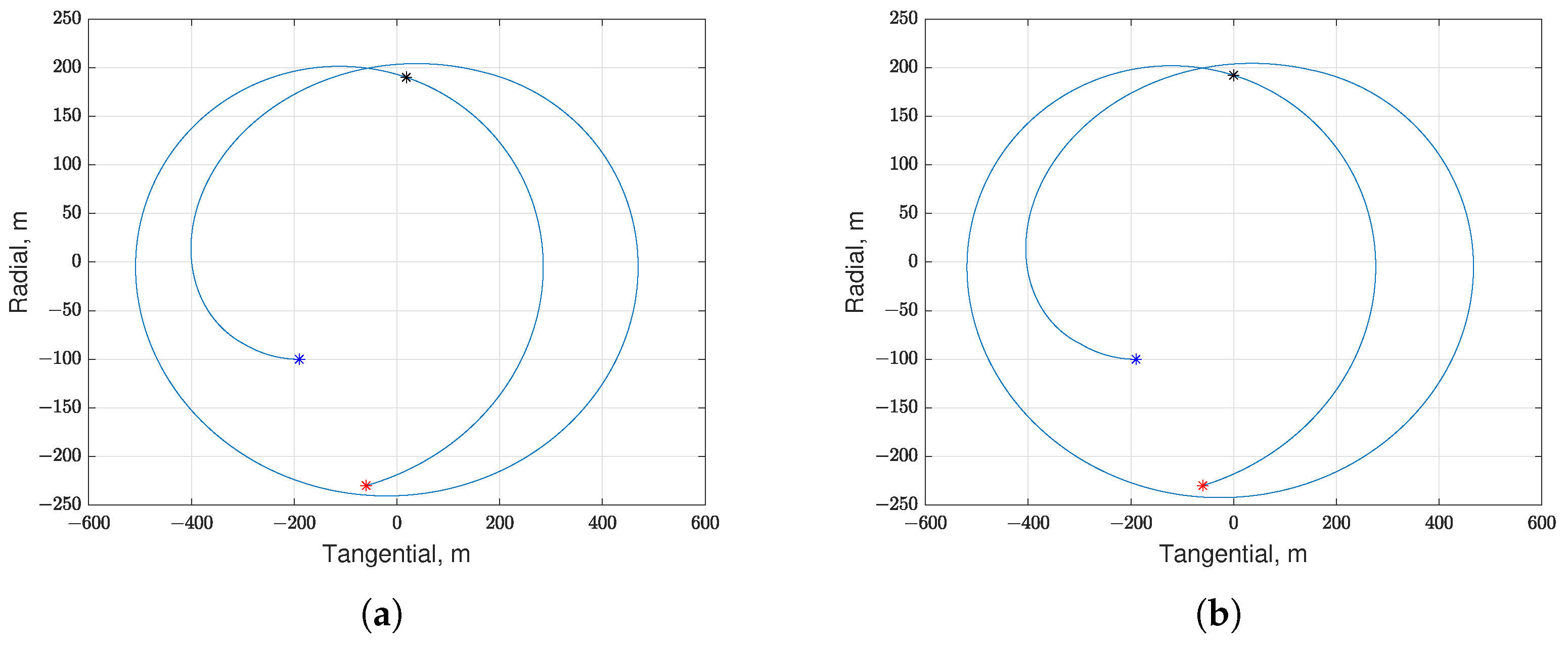
Figure 12a shows the unconstrained relative path and Figure 12b depicts the corresponding constrained trajectory. The position vector at the specified time instant corresponding to $u=\overline{u}$ is marked with black asterisks, while red and blue asterisks represent the initial and final relative position vectors, respectively.

The second example concerns collision avoidance. In the context of relative orbital elements, these requirements are commonly met through passive strategies based on the concept of separating eccentricity and inclination vectors, a principle derived from the collocation of geostationary satellites [26]. Notably, our formulation not only enables the derivation of passive strategies, but also facilitates the computation of collision avoidance maneuvers. To illustrate this, we establish the condition that the deputy spacecraft must operate on or beyond the boundaries of a spherical forbidden region with radius $R_{ca}$ centered around the target, that is,

$${\overrightarrow{y}}^T\overrightarrow{y}\ge R_{ca}.$$

(47)

The planar reconfiguration problem is again taken as example and $R_{ca}=200 \mathrm{m}$. If Scheme 1 solution enters the forbidden region, the refinement is again tweaked to account for the constraint. Given the reference mean argument of latitude $\overline{u}$ of the minimum distance point in the unrefined solution (red point in Figure 13a), with the corresponding position vector ${\overrightarrow{y}}_{ref}$, Equation (47) is linearized and

$${\overrightarrow{y}}_{ref}^T\overrightarrow{y}=R_{ca}\left|{\overrightarrow{y}}_{ref}\right|$$

(48)

is added to the problem constraints to solve the KKT equations. Linearization of Equation (47) introduces errors, and the accuracy index of the solution is expressed as

$$|\overrightarrow{y}\left(\overline{u}\right)-\overrightarrow{y}{\left(\overline{u}\right)}_{ref}|.$$

(49)

When $\overrightarrow{y}$ exhibits relevant changes, the constraint may still be violated, but, in this case, the accuracy improvement to a satisfactory level can be easily accomplished by iteratively solving the KKT system of equations where the reference trajectory is set equal to the solution obtained in the preceding step.

Figure 13b shows that the constrained optimization leads to a feasible trajectory and the relative distance $r\left(u\right)=|\overrightarrow{y}\left(u\right)|$ never falls below the pre-established threshold $R_{ca}$.

It is important to note that all the procedures delineated in this section can be directly applied to three-dimensional transfer by considering Schemes 3 and 4 in Section 3. Moreover, the effective handling of multiple constraints can be easily addressed by introducing additional impulses where necessary. While outside the current scope of this work, this section offers insights into the potential for addressing typical mission constraints. Future efforts will be devoted to a more comprehensive analysis of the extendability of our algorithms.

6. Conclusions

We proposed four simplified analytical strategies to solve complex proximity operations problems comprising significant changes in the relative mean longitude and three-dimensional reconfiguration. The analytical nature of the solutions ensures that computational times are negligible when compared to the typical scales of reconfiguration maneuvers. As a result, these strategies guarantee real-time capabilities and can be employed alongside existing approaches (e.g., those used in the AVANTI demonstration) to choose the optimal solution for a given scenario. Furthermore, when a more complex numeric optimization procedure is necessary for higher accuracy, the solutions proposed here may offer tentative solutions and valuable insights for planning relative trajectories and solving the problem of relative motion reconfiguration with additional fidelity.

Results for the planar case show that percentage difference of the cost indexes of our scheme and the optimum is always less than 3.5%. The proposed strategy focuses on problems with a dominant change in mean longitude and outperforms existing strategies not specifically designed for these types of transfers (averaged $\Delta V$ savings of $49.88$%). Our algorithm is also proven to be flexible enough to almost reach the global minimum propellant consumption when the relative semi-major axis or the relative eccentricity vector dominate the reconfiguration.

The different schemes proposed for the three-dimensional reconfiguration problems show the benefit that may be obtained by combining in-plane and out-of-plane maneuvers. This versatility allows for (almost) optimal performance in terms of propellant consumption, but it may also offer hints for the general theoretical understanding of 3D reconfiguration (e.g., how the plane change is best split between impulses, when impulse combination is most beneficial, etc.). In addition, the availability of different analytical algorithms able to solve the same 3D reconfiguration problem allows for a better management of practical time windows, in which mission requirements may impose the absence of maneuvers. Such requirements could be easily tackled with small tweaks to the algorithms.

Even if this paper deals with near circular reference orbits, the mapping from impulse components to ROE changes can be generalized for elliptic orbits [21], whereas the state transition matrix remains the same. In principle, the method can readily be extended to this case. However, the optimality of the proposed schemes is not guaranteed, and investigation of different strategies could be required. Extension to elliptic orbits is left for future work.