1. Introduction
Historically, the development of aircraft has depended on the combined use of empirical data, experimental testing, physics-based models, and simulations. But, as practitioners seek to develop unconventional aircraft or designs that have little to no historical data, the use of physics-based models has become integral to the design process. Moreover, rather than relying solely on integrated parameters, such as lift or drag coefficients, to quantify the high-level performance of the system, it is crucial to consider the spatio-temporal distribution of quantities, such as pressure over the wing, to guide decision making. These distributions are often referred to as fields and may have thousands to millions of data points, which can be used to obtain integrated parameters. Understanding and accurately analyzing these high-dimensional fields, including the strength, shape, position, and variation of nonlinear features within them, such as shocks, is vital to optimizing the structural, aerodynamic, and aeroelastic performance of the aircraft. Physics-based models not only enable the precise determination of these features and their variations to design changes, but also reduce program costs and accelerate the time to production.
However, depending on the field being evaluated, it may be greatly impacted by geometry changes, uncertainties in flight and atmospheric conditions, and variations in the manufacturing process. Ideally, the design of aircraft would not simply account for these uncertainties, but also focus time and resources to enhance system robustness. Uncertainty quantification (UQ) refers to the process of propagating the impact of these changes in uncertain parameters through the system to calculate statistical moments, such as expected value and standard deviation, and obtain output distributions on key performance metrics. The Monte Carlo (MC) method is the standard approach for performing UQ, but it suffers from slow convergence rates and requires a significant number of samples to accurately model the system. For computationally expensive analyses, their limited sampling budget poses a practical challenge for such MC-based approaches. Thus, there is a need to develop a methodology to not only efficiently propagate uncertainty, but also do so in high-dimensional fields to enable robust design.
1.1. Surrogate Modeling
In the literature, there exist several methods to reduce the computational cost of MC and enable UQ. One example is to reduce the number of samples needed for MC by omitting certain variables. This approach is followed in [
1], where the authors explore the sensitivity of variables to uncertainties, but use prior knowledge about the simulation to remove certain variables. This strategy, though powerful when the dynamics of the system are well understood, is unsuitable for simulations where the practitioner has little or no prior knowledge. In such cases, reducing variables may lead to the loss of valuable information and insights, limiting the effectiveness of the UQ procedure.
An alternative to this approach is to use adjoint-based methods, which rely on analytical equations to calculate sensitivities of outputs with respect to inputs. This is commonly used in robust design and optimization where the goal is to generate designs that are resilient to uncontrollable variations. There, the purpose of uncertainty propagation is to obtain expressions for the sensitivity of the outputs to uncertain parameters. In such cases, this adjoint-based formulation enables a drastic reduction in computational cost [
2]. However, one significant challenge of these methods is that they require substantial code modifications to implement the adjoint equations. Often, software packages and simulation tools utilize proprietary solvers which cannot be modified or even accessed, severely limiting the usability of adjoint-based methods.
A common option that overcomes the limitations of the above methods is surrogate modeling. In this approach, the practitioner first builds a mathematical approximation of the underlying system being analyzed and then uses this cheap-to-evaluate model to perform MC. While there exist a variety of approaches to perform surrogate modeling in UQ [
3,
4], this study focuses on polynomial chaos expansions (PCE).
PCE models rely on a set of predefined orthogonal basis functions to express the output random variable by separating its deterministic and stochastic contributions. PCE boasts a robust mathematical foundation rooted in probability theory and provides guarantees on error convergence rates [
5,
6]. More important, the coefficients of a PCE surrogate model can be used to analytically obtain precise estimates for statistical moments and Sobol sensitivities without the need for MC simulations. This not only reduces the overall sampling cost, but also prevents the accumulation of additional errors. Given these strengths, this study explores the use of PCE for high-dimensional UQ problems. For the past two decades, PCE has been widely adopted and extensively studied in capturing and handling scalar stochastic variables. However, the application of PCE to high-dimensional stochastic simulations which produce millions of correlated random variables is still challenging and an active area of study. Hence, the discussion below focuses on methods for performing UQ in high-dimensional spaces.
1.2. Reduced Order Models
Reduced order modeling is a data-driven surrogate modeling method to efficiently handle high-dimensional data and approximate a complex simulation. The core concept behind ROM is that the high-dimensional data exist on some lower-dimensional space, which captures all the essential features of the problem. ROMs strive to identify this low-dimensional space and employ it to predict solutions at unseen points, all while keeping computational costs low. Using a process known as dimensionality reduction, ROMs not only compress the data into a smaller, low-dimensional space, but also maintain spatial coherence within the model. Further, since ROMs provide estimates of the entire spatio-temporal field, they can be used to predict all downstream integrated quantities of interest.
The proper orthogonal decomposition (POD) method is a linear method for dimensionality reduction and has been predominantly used for ROMs due to its simplicity. Over the past decade, researchers have attempted to combine POD-based approaches with PCE to enable UQ in high-dimensional problems. For example, Raisee et al. [
7] developed a POD approach to reduce the high cost associated with training PCE models (discussed further below), but still relied on fitting a scalar-PCE model at each node in the computational mesh. Moreover, as noted by several researchers [
8,
9], Raisee’s method still relies on expert knowledge and can be viewed as a variant of a scalar surrogate model, introducing inconsistencies in spatial coherence.
Recently, some researchers have explored the use of POD to first reduce the dimensionality of the problem and then construct a PCE model in the latent space to capture the dynamics of the stochastic simulation. The application of this method has however largely been restricted to problems with small degrees of nonlinearity or benchmark problems from mathematics [
10,
11,
12,
13,
14,
15,
16]. An assessment of the performance of these models in problems with discontinuities, nonlinearities, and real-world engineering datasets is necessary prior to their adoption in the aircraft conceptual design process. Therefore, the combination of POD and PCE remains a subject requiring further investigation.
1.3. Contribution of the Paper
This study leverages the POD–PCE method in uncertain aerodynamic problems with possibly millions of outputs. Specifically, the problems addressed are from computational fluid dynamics (CFD) simulations designed to resemble those seen in supersonic and transonic aircraft design, where aerodynamic solutions can have several localized nonlinear, discontinuous features, such as shocks. To the knowledge of the authors, a comparison of POD–PCE with Monte Carlo results for real-world aircraft in supersonic or transonic CFD simulations has been unexplored in the literature. More broadly, given that the previous literature has mostly been confined to linear problems, this would provide empirical insight into the performance and robustness of POD–PCE in non-trivial problems encountered often during aerodynamic design. Through methodical demonstration, the research showcases a comprehensive characterization of the ROM in accurately and efficiently predicting statistical moments and point predictions at a fraction of the original computational cost.
The conclusions drawn from these experiments will not only offer new perspectives for the fields of ROM and UQ but also contribute to the advancement of robust aircraft design methodologies.
The structure of the manuscript is as follows:
Section 2 provides an overview of the POD and PCE methods.
Section 3 outlines the UQ methodology with error metrics.
Section 4 discusses the performance of the method in three test cases and
Section 5 summarizes key findings and next steps.
2. Reduced Order Modeling
The sections below provide the underlying theory and numerical details for proper orthogonal decomposition and polynomial chaos expansion.
2.1. Proper Orthogonal Decomposition
The POD method is renowned for its simplicity and has been used not only in aerospace engineering, but also in numerous other fields, such as statistics and computer science. The fundamental concept behind POD is to identify a linear subspace using the principal component vectors or singular vectors of the training data supplied. These vectors are obtained using Singular Value Decomposition (SVD) and identify those directions in the high-dimensional vector space that best capture the variance of the outputs. In approximating the Full Order Model (FOM) with this reduced order approximation, the computational cost is drastically reduced.
To begin, assume that there exists some deterministic model
which acts on a set of inputs,
, and yields some vector output,
∈
. Consider a matrix,
, that consists of
m training vectors obtained at
m input parameters. For simplicity, but without loss of generality, assume that the matrix is mean-centered:
The SVD algorithm applied to this matrix results in:
where
is the matrix of POD modes,
is a matrix of right singular vectors, and
is a diagonal matrix of singular values, such that
and
.
The next step is to identify the
d most dominant POD modes using a measure like the Relative Information Content (RIC). The RIC is defined as:
Most often, the practitioner sets the RIC to some
, then selects
d basis vectors such that RIC
. A matrix spanned by the
d most dominant POD modes is then constructed:
. Having obtained this matrix, each snapshot is then projected onto the reduced space:
where
is the matrix whose columns correspond to each snapshot’s coordinates in the latent space, such that
. Each
is then paired with its associated set of input parameters,
, and used to train a scalar regression model.
2.2. Polynomial Chaos Expansion
Polynomial Chaos Expansion is a method for uncertainty quantification that separates a random variable into its deterministic and stochastic contributions using a linear combination of orthogonal polynomials [
17].
Suppose that represents a full-order model which acts on a set of uncertain random variables and yields a field. Let be a random field where each spatial location is a scalar random variable and is determined by random inputs that form a random vector.
For each
, one selects a family of polynomials
with a polynomial order,
. Define the inner product:
For each random variable, using the underlying probability density function (PDF),
, it is possible to derive an associated set of orthogonal polynomials,
, that satisfy
where
is the Kronecker delta. Xiu and Karniadakis [
17] found the orthogonal polynomial basis for common PDF distributions. These are summarized in
Table 1 and offer exponential convergence rates of error for statistical moments [
5,
6].
By multiplying the polynomial basis for every input variable with every other variable’s basis, one obtains the following multivariate basis, which is orthogonal with respect to the joint probability distribution of all the inputs:
Using this multivariate polynomial basis, it is possible to express
:
where
are deterministic coefficients that vary with
.
As was done with POD, the practitioner typically truncates the infinite expansion to some order
P depending upon the accuracy sought.
A common way to truncate the expansion is to set an upper bound on the total degree of the polynomial expansion to
p such that
Thus, the total number of terms in the expansion is given by .
Since the PCE model is constructed using orthogonal polynomials, statistical moments can be obtained using closed-form expressions:
and
Having established the underlying theory for PCE models, the discussion below focuses on the numerical details of the non-intrusive training procedure.
Collocation-Based PCE
During implementation, the estimation of the PCE coefficients can be accomplished using different techniques such as Galerkin approaches, quadratures, and stochastic collocation. The reader is referred to [
18,
19] for a thorough overview of the various methods for determining the PCE coefficients. The discussion below provides a brief review and the implementation details for stochastic collocation methods.
The Galerkin procedure is part of a family of methods known as intrusive methods, all of which require modifications to the underlying FOM. Since this is unsuitable for black-box codes, it is not explored below. Quadrature methods involve collecting samples at specific integration points in the domain. However, this approach may request samples at points in the domain where the simulation cannot converge to an answer (which can occur frequently with CFD simulations at high angles of attack or complex geometries with complicated flow patterns). Stochastic collocation, alternatively referred to as regression-based PCE, is a robust, cost-effective approach to perform PCE with black-box tools.
Stochastic collocation starts by generating
samples of the random vector
, which are used to acquire snapshots of the FOM. Since each element of the field is a random variable, for simplicity, the discussion below focuses on scalar outputs. However, these approaches can be readily extended to fields with millions of random variables. The coefficients
can be found by solving the following over-determined linear system:
The procedure above requires a minimum of
points to ensure a solution exists. It is common to use an oversampling of at least twice more than the required points as this yields a better approximation for the statistical moments [
20]. The formulation above uses an
-norm, but this study also explores the use of sparse methods which employ least angle regression to determine the most significant PCE coefficients [
21].
The two research domains of UQ and ROM have developed several techniques which have strong parallels. Recently, the combined usage of UQ and ROM has been an active area of research.
3. Methodology
The section below introduces the POD–PCE method, which is a parametric, non-intrusive ROM technique to propagate user-defined uncertainties to high-dimensional fields. In general, the procedure can be decomposed into two phases: the offline phase, where the model is trained, and the online phase, where the model is used to predict uncertain fields for unseen parameter points. During the offline phase, the following steps occur (see Algorithm 1):
The uncertain parameters, , are identified, and the underlying probability density function for each random variable, , is defined.
A design of experiments (DOE) is used to sample m combinations of design variables, , and the FOM, , is evaluated to generate the solutions of the random field.
The matrix of snapshots, , is generated, and the POD procedure is employed to construct a low-dimensional embedding, . The dimensionality of the latent space is based on the desired threshold, , such that of the data.
A multivariate PCE model is used to learn the dynamics of each stochastic latent space coordinate, , to obtain such that . This parameterizes the latent space.
During the online phase, the multivariate PCE models are used to first predict the latent space coordinates at some specified input parameter, , using . Then, the POD modes are used to transform the embedded coordinates to the full-dimensional space by the projection .
The above training procedure results in the following model:
where
and
are the PCE and POD basis functions, respectively. This formulation highlights that the model is a linear combination of POD modes; the coefficients of those modes are determined by a PCE expansion.
Figure 1 provides a visualization of the training process.
Note that once the PCE models are built in the latent space, the coefficients of the polynomials can be readily used to obtain the mean, standard deviation, and any statistical moment of the reduced space analytically. Once these latent space moments are calculated, the POD modes can be used to map them to the high-dimensional space. For example, the mean can be analytically computed as follows:
This capability of rapidly and analytically obtaining moments without the need for further MC simulations is a primary benefit of the POD–PCE method.
| Algorithm 1: Offline ROM Algorithm |
Input: - 1
Utilize DOE to generate m samples of input uncertainties, - 2
Construct snapshot matrix, , using FOM evaluations - 3
Perform dimensionality reduction to identify latent space coordinates - 4
Train regression models for each latent space coordinate, , to obtain such that - 5
Return and
|
The analysis below uses several error metrics to characterize the performance of the ROMs. In general, the error metrics can be decomposed into scalar and vector metrics. The scalar metrics enable the rapid comparison of one model to another by providing one numerical value that measures accuracy. On the other hand, the vector metrics provide a visual representation of the error for a particular model over the entire computational domain. This allows the practitioner to determine regions of the domain where the models deteriorate in accuracy.
The root mean square error (RMSE) is one vector metric that provides an assessment of the overall predictive performance of the models over the entire validation set. This error is evaluated at each node in the
—dimensional computational mesh across all
test cases. Each component of this vector can be determined using:
where
is the predicted solution from the ROM and
is the exact FOM solution at the
ith node for the
jth test case.
To visualize the discrepancy for a particular test case, the following error metric can be defined:
Note that this metric can be used to compare the predicted moments from the ROM to those obtained using the FOM. Suppose that the mean field predicted using the ROM is denoted as
. Then, the error between the predicted solution to the exact FOM mean,
, is:
Having established the vector metrics, the normalized RMSE (NRMSE) will be used as a scalar measure to assess the overall accuracy across ROMs:
NRMSE can be decomposed into a reconstruction and regression error. The former measures the error introduced by the dimensionality reduction procedure, while the latter measures the error from the PCE models. The reconstruction error is given by:
The regression error is given by:
where
is the predicted latent space coordinate found using the PCE regression models.
Lastly, a scalar metric using the
-norm will be used to compare statistical moments:
4. Experimentation and Results
The empirical investigation below sheds novel insight into the behavior of the linear UQ procedure when applied to engineering datasets that may be encountered during aircraft design. These test cases include uncertain flow inside a converging-diverging nozzle, over a 2D airfoil, and over a 3D geometry. In each case, the flow field is high-dimensional, with at least 1000 random variables and as large as 77,000 variables in the 3D case. Further, the solutions are obtained using CFD solvers that either use the Euler equations or Navier–Stokes equations, which are second-order nonlinear partial differential equations. The geometry and boundary conditions are set such that there is a localized region of supersonic flow in each solution that results in expansion fans and shockwaves, further increasing the complexity of the underlying model. Lastly, the number of inputs is increased from one to three as the training data are varied to test the performance in multiple input parameter problems. Thus, these experiments are tailored to meticulously assess the proposed method in practical problems and establish its advantages and disadvantages for future practitioners.
4.1. Converging-Diverging Nozzle
The first experiment addresses a simplified test problem with uncertain flow through a converging-diverging nozzle due to geometry changes. The governing equations for the FOM are
where
is the area distribution,
is density,
p is pressure,
u is velocity, and
is the specific heat ratio of the fluid. Uncertainty is introduced in the problem through changes in the throat area (
) which impact the pressure ratio through the nozzle. The nozzle has a parabolic shape whose cross sectional area changes from
, with the throat located at
. The throat area varies as a uniform random variable on the interval [0.75, 1]. Using the boundary conditions,
and
, the governing equations are solved using a finite difference procedure over a uniform grid with 1000 nodes. This results in a shockwave inside the nozzle. A Latin Hypercube Sampling (LHS) DOE is used to generate
m samples for training and
for testing. The training set is varied in size (
) to evaluate the impact of sampling density on prediction results.
The variation of the pressure distribution inside the nozzle for different uncertain parameters is shown in
Figure 2. It is seen that the size and location of the shockwave depends on the throat area. Equally important, the pressure value after the shock is dependent on the strength of the shock. Thus, the accurate prediction of the flow field requires both the precise determination of the large amplitude changes in shocks and the smooth pressure variation at all other points.
Figure 3 illustrates the test case responses predicted using the ROM for both a low-order and high-order PCE model. The results demonstrate that the POD–PCE model can accurately predict responses away from the shock region, but exhibits significant errors near the shockwave. Specifically, the solution exhibits overshoots and undershoots and errors persist in locations away from the actual discontinuity. Increasing the PCE order decreases the magnitude of the error, but higher-frequency oscillations appear near the shock. This behavior is referred to as the Gibbs phenomenon [
22], and is expected to occur since the PCE model may not be able to capture the latent space accurately [
23].
To better understand the effectiveness of the ROM, it is possible to analyze the latent space identified after dimension reduction.
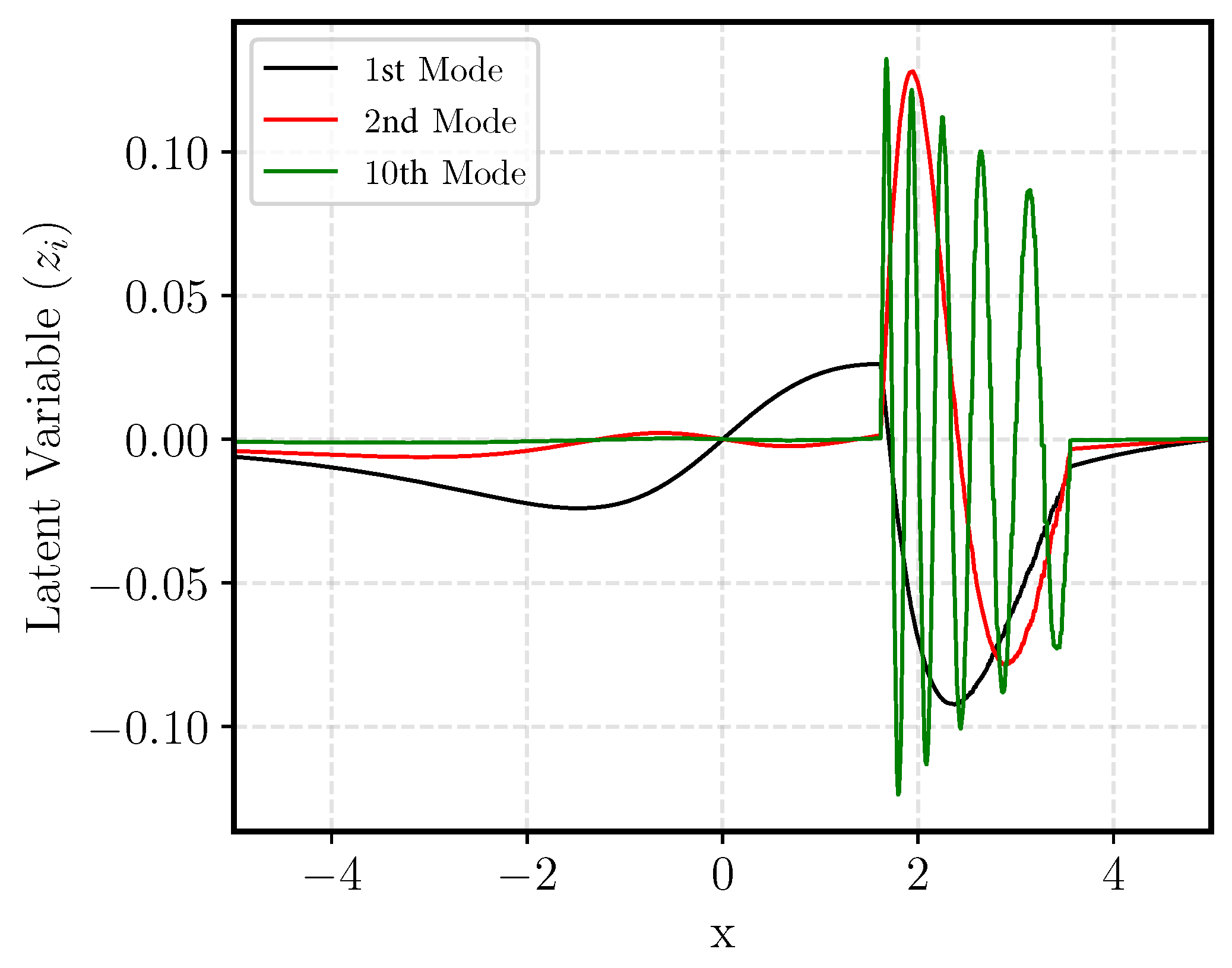
Figure 4 shows some of the POD modes identified. In general, it is seen that other than the first mode, most of the variations have high frequency. These modes are associated with the sharp discontinuity and contribute to the oscillatory behavior seen in the above plots. This necessitates the use of higher-order PCE models, but, even with a fifth-order regression, a large portion of the shockwave variation may not be precisely captured. To verify this,
Figure 5 shows the predictive performance of the PCE models for the first and tenth latent space coordinates. It is observed that the PCE model is able to capture the low-order dynamics of the first latent space coordinate. On the other hand, the tenth POD mode has an extremely nonlinear latent space, requiring a large number of PCE coefficients to fit it. These discrepancies manifest as oscillations and highlight the importance of precisely predicting the dynamics in the latent space.
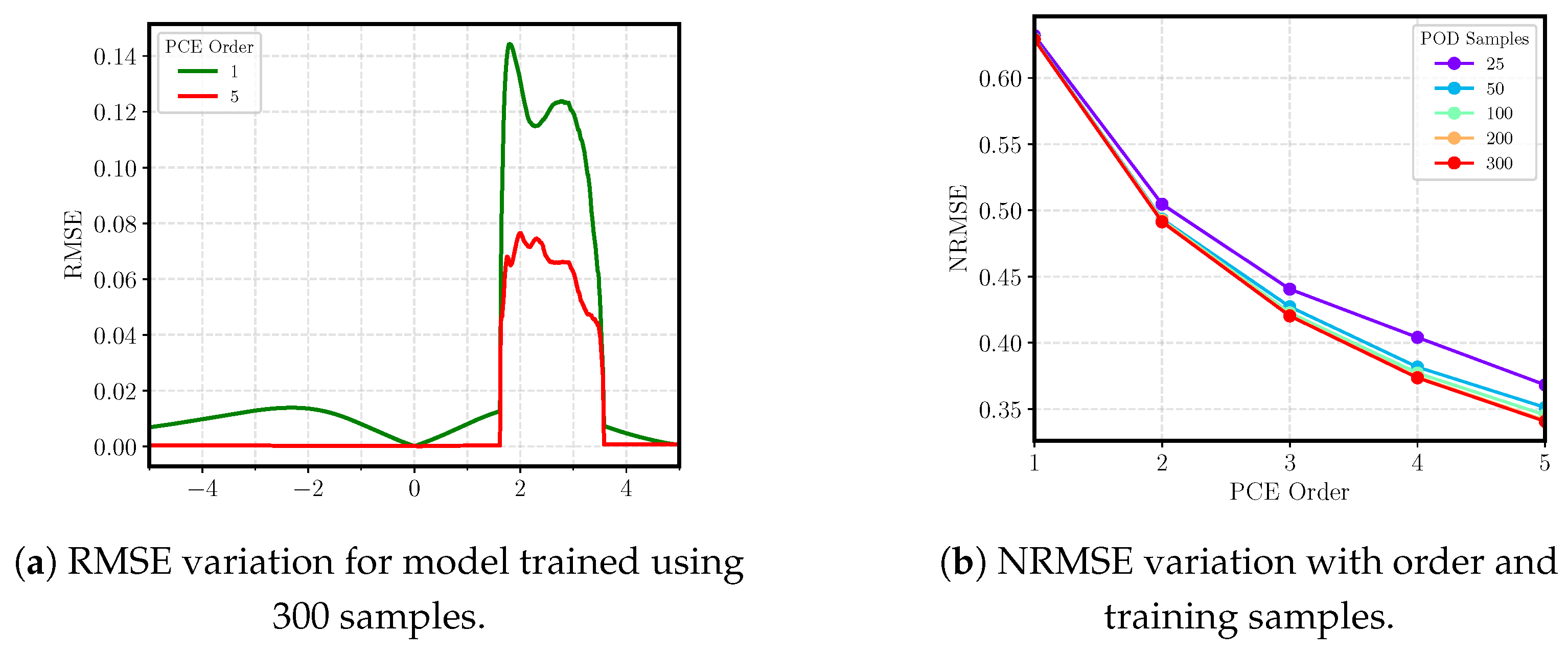
Figure 6 provides a visualization of the RMSE for ROMs trained using 300 samples but with different PCE regressions. The low-order model exhibits consistently high errors, not simply near discontinuities but also in the regions without shocks. As the order increases, the regression model better captures the dynamics of the latent space. This diminishes the error in the regions away from the shock, but the solution continues to exhibit oscillations near the discontinuity.
Figure 6b provides a more refined assessment of error as the PCE order increases. Though errors monotonically decrease with increases in the PCE order, there is no clear asymptote, which indicates that even the largest PCE model is insufficient to accurately model the latent space. This is because flows with shockwaves have a slow eigenvalue decay and thus a large number of POD modes are required to meet the relative information content threshold of 99.99%. However, as additional singular vectors are added to the POD basis, the regression procedure becomes more complex. Thus, a higher-order PCE model is required during training. Similarly, increases in the samples provided during training also decrease the error, though with only marginal improvements. Since the NRMSE is more impacted by the PCE order than the number of samples, it is once again seen that the regression model cannot predict variations of the embeddings.
Figure 7 shows the variations in the reconstruction and regression error that contribute to NRMSE. It is observed that increasing the number of samples from 25 to 100 reduces the reconstruction error by over 50%. Further increasing the samples does result in an error decrease, though with diminishing returns. The PCE order and reconstruction error are independent of one another. Note that the number of POD modes required to capture the RIC increases rapidly with training samples (see
Table 2). Consequently, for a fixed PCE order, regression errors increase with more sampling data, given the increasingly nonlinear and higher-dimensional nature of the latent space. Thus, any improvement to the regression procedure that would have been obtained with the additional training data is nullified by the increasing complexity of the latent space. In fact, the regression error contributes more than 75% of the NRMSE, reflecting the latent space modeling challenges. Thus, the hypothesis that the regression error, and therefore the PCE model’s limitations, contribute more significantly to the NRMSE than the reconstruction error is supported.
Figure 8 presents statistical moments calculated through Monte Carlo analysis using the FOM and those obtained using analytical expressions for PCE coefficients. The FOM results shown utilize a bootstrapping procedure with 500 re-samples to obtain confidence intervals for the moments, but the confidence interval is small enough that the solutions collapse onto one curve. The mean response shows a gradual pressure change that is a byproduct of averaging the discontinuous jumps in pressure across samples. The variance plot shows that the largest changes occur between
because the shockwave exhibits the most significant variation within this range. The results show that when the mean is calculated analytically, it perfectly matches the MC results. Note that the convergence of the moments calculated using MC to the exact moments is slow. Specifically, it can be shown that the error for MC drops with a rate of
, where
m is the number of samples. POD–PCE avoids this additional MC cost and yet maintains precision, and therefore is a powerful tool for uncertainty propagation. While increasing the order improves the accuracy of predicting the variance, a fifth-order PCE model still cannot predict the maximum variance.
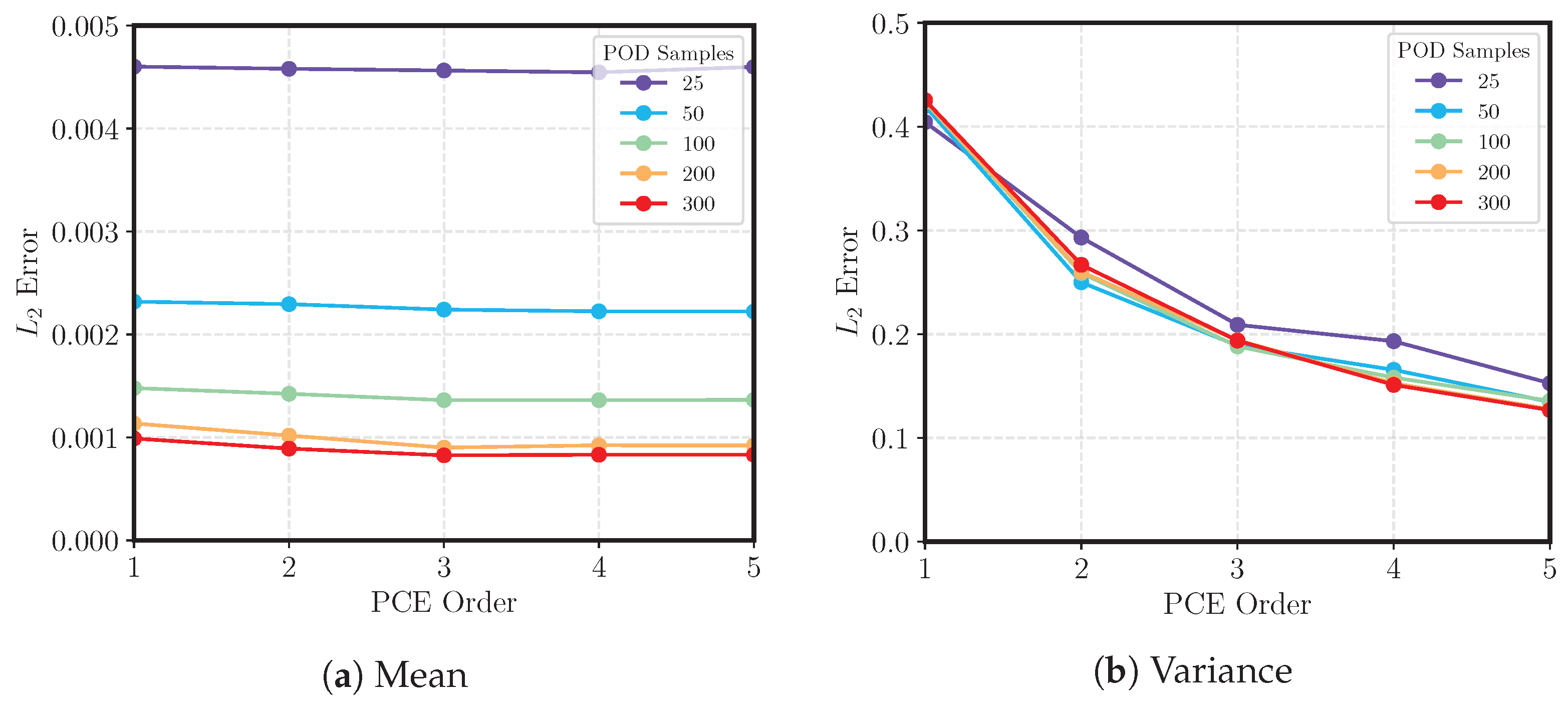
Figure 9 depicts the impact of different training samples and PCE orders on the relative
-norm errors in the mean and variance. In both figures, an increase in the samples leads to a decrease in error. More important, the POD–PCE method can accurately estimate the mean response, and the error is largely unaffected by the order of regression. This indicates that a sparse POD–PCE model is able to not only create parsimonious models, but also maintain the salient features of the problem for analytical computation of moments.
Note that the integrated error for variance is two orders of magnitude larger than that of the mean. To minimize variance error, high-order PCE models should be used. However, it is equally important that this be accompanied with an increase in RIC during dimensionality reduction. The RIC used to truncate the POD modes during dimensionality reduction measures the amount of variance captured by the low-dimensional subspace. Thus, the maximum accuracy for a POD–PCE model’s variance prediction is set during the POD truncation phase. For flows with discontinuities, which have slow eigenvalue decay, an RIC near 1 improves the variance and shock prediction, but drastically increases the number of POD modes retained.
Lastly, since the discussion above has focused on the accuracy of the models over the entire field, it is important to also assess the performance at specific points in the computational domain. Each point would represent a scalar random variable and would have an associated distribution.
Figure 10 shows the distribution obtained from the FOM and the ROM at two points in the domain. The first location is at
, where the flow has no discontinuities. It is seen that the ROM is able to perfectly reconstruct the variation and distribution of the outputs without any inconsistency. On the other hand, at
, the flow varies significantly due to the presence of the shock and the model is unable to predict the discrete jump. The linear model smooths this distribution. Thus, it can be concluded that the performance of POD–PCE is accurate in flows where the shockwave is restricted to a small portion of the domain or in regions where the shockwave does not exist.
4.2. RAE2822 Airfoil in Transonic Flow
The following experiment for uncertain transonic flow over an RAE2822 airfoil further increases the complexity of the problems in three ways: First, the number of inputs increases from one to three, which makes the latent space regression more challenging. Second, the underlying governing equations are now the Navier–Stokes equations solved with turbulence models, which make both the dimensionality reduction and regression step difficult. Third, the flow domain itself is 2D and has 10 times the number of random variables. Moreover, the field has mixed supersonic and subsonic flows and shockwaves that vary in size, shape, strength, and location. Thus, this experiment adds significant, novel empirical insight into the performance of POD–PCE in real-world aerodynamic simulations that may arise during conceptual design or aerodynamic shape optimization.
The FOM used in this simulation is a Reynolds-Averaged Navier–Stokes (RANS) CFD solver, SU2. A Spalart–Allmaras (SA) turbulence model is used to resolve the viscous effects over an O-grid mesh with 10,500 nodes. An RAE2822 airfoil is parameterized using the Free-Form Deformation (FFD) approach, whereby a bounding box around the airfoil is used to perturb its shape [
24]. Uncertainties are introduced by defining two control points at the mid-chord of the airfoil and independently changing their vertical displacement from the baseline by
of the chord length. Perturbations from the baseline are uniformly distributed. The angle of attack is also an uncertain parameter, which varies uniformly over the interval [−
,
]. The freestream Mach number is fixed at 0.725 for all simulations, resulting in a shockwave either on the upper or lower surface.
An LHS DOE with 2500 points is used to sample the FOM. From this set, 60% of points are randomly selected to be a part of the validation set and the training dataset is varied such that . In doing so, the impact of sparse training data on overall performance is evaluated as was done in the previous test case.
Figure 11 compares the accuracy of the ROM to the CFD solution for a case from the validation set. The POD–PCE method accurately predicts the pressure distribution around the body in regions with fully subsonic flow. However, near shockwaves, the error steadily increases and is largest near the actual discontinuity location. This large region of localized error is due to the imprecise prediction of the shock shape and location and also due to the presence of Gibbs oscillations. Since the POD–PCE model performs well in the purely subsonic regions, it can be hypothesized that the method is most proficient in problems where shockwaves are a small fraction of the overall solution or when discontinuities are absent. The last experiment investigates whether this accuracy is maintained in purely supersonic flows over 3D bodies.
When the performance is inspected across the entire validation set (
Figure 12), the limitations of the linear methodology become clearer. The RMSE is nearly 0 throughout the computational domain, except on the upper surface where the shock varies most. As the regression order is increased, the RMSE steadily decreases and the region of error shrinks significantly in size. In fact, when a first-order model is used, both the upper and lower surfaces have a large RMSE, while a fifth-order model restricts the error to the mid-chord of the upper surface. This is because an increase in the regression order improves the latent space prediction of all modes, but especially assists with the prediction of the trialing modes that are associated with the shock dynamics. Quantitatively, as the PCE order increased, the maximum RMSE decreased by nearly 50% from 0.144 to 0.76. This performance improvement is reflected in the NRMSE plots in
Figure 13a with a decrease in error of 61%.
Further, when the training data points are increased, the NRMSE consistently decreases, though with diminishing returns. This is because the oversampling ratio increases and improves the accuracy of the PCE coefficients. It is worth noting that the number of modes does not change after 200 training samples (see
Table 3), thus fixing the dimensionality of the latent space. As such, any improvement in NRMSE beyond 200 samples is purely due to improvements in the regression procedure and minor changes in the accuracy of the POD modes. As the PCE order is increased, the differences between the ROMs become amplified and there is a monotonic decrease in error. Specifically, for sparse datasets, there is a rapid asympotote in the regression error as the PCE order increases. For larger ones, the asymptote is delayed and error continues to diminish because of the availability of more training data without an increase in the number of POD modes. This behavior is seen for all sample sizes except when 50 training data points are supplied. For this case, the slight increase in error when the PCE order is increased beyond a quadratic model is because the oversampling ratio falls below 2. In fact, a fifth-order model requires at least 56 samples, but with only 50 supplied, the problem becomes underdetermined and the solution is inaccurate.
Figure 13 also displays the variations in reconstruction and regression errors. The reconstruction error is an order of magnitude smaller than the regression error, reflecting the challenge of the PCE model in predicting the latent space variations. As the sample size increases, the reconstruction error decreases, although it saturates beyond 300 samples, indicating that the additional data supplied add minimal novel information to the POD modes. Similar to the trends seen in the CD Nozzle test case, the regression error dictates the performance of the NRMSE and supports the conclusion that the linear assumptions used within PCE (although beneficial for analytical moment computation) are a hindrance to the effectiveness of POD–PCE.
Finally, note that in the first test case, the number of nodes retained was nearly eight times larger than the current test case (see
Table 2). This can be attributed to the fact that the shock occupies a smaller fraction of the overall computational domain. Consequently, a smaller number of POD modes are required to meet the RIC and the NRMSE is also lower (even though the number of nodes is 10 times larger). Together, these findings further support the hypothesis that POD–PCE models perform well in simulations with few discontinuities or when the nonlinearities are restricted to a small fraction of the domain.
Figure 14 and
Figure 15 present a comparison of the statistical moments. Since the geometry changes, the results shown are overlaid on the baseline airfoil at zero angle of attack. In both sets of plots, the error is largest near the shockwave. The analytically calculated mean closely matches the FOM and is unaffected by the PCE order. The variance, being much harder to predict, has errors that are an order of magnitude larger. The flow has the largest variation in pressure coefficient near the leading edge and on the upper surface of the airfoil. However, the error is restricted to the upper surface and reaches a maximum value at the shock location. This suggests that even if the variance is high, the POD–PCE method can predict it accurately. However, if the variations are accompanied by or due to shockwave movements, there is rapid decrease in precision as the ROM exhibits the Gibbs phenomenon. As expected, as PCE order increases, both the extent of error and its magnitude decrease for the variance.
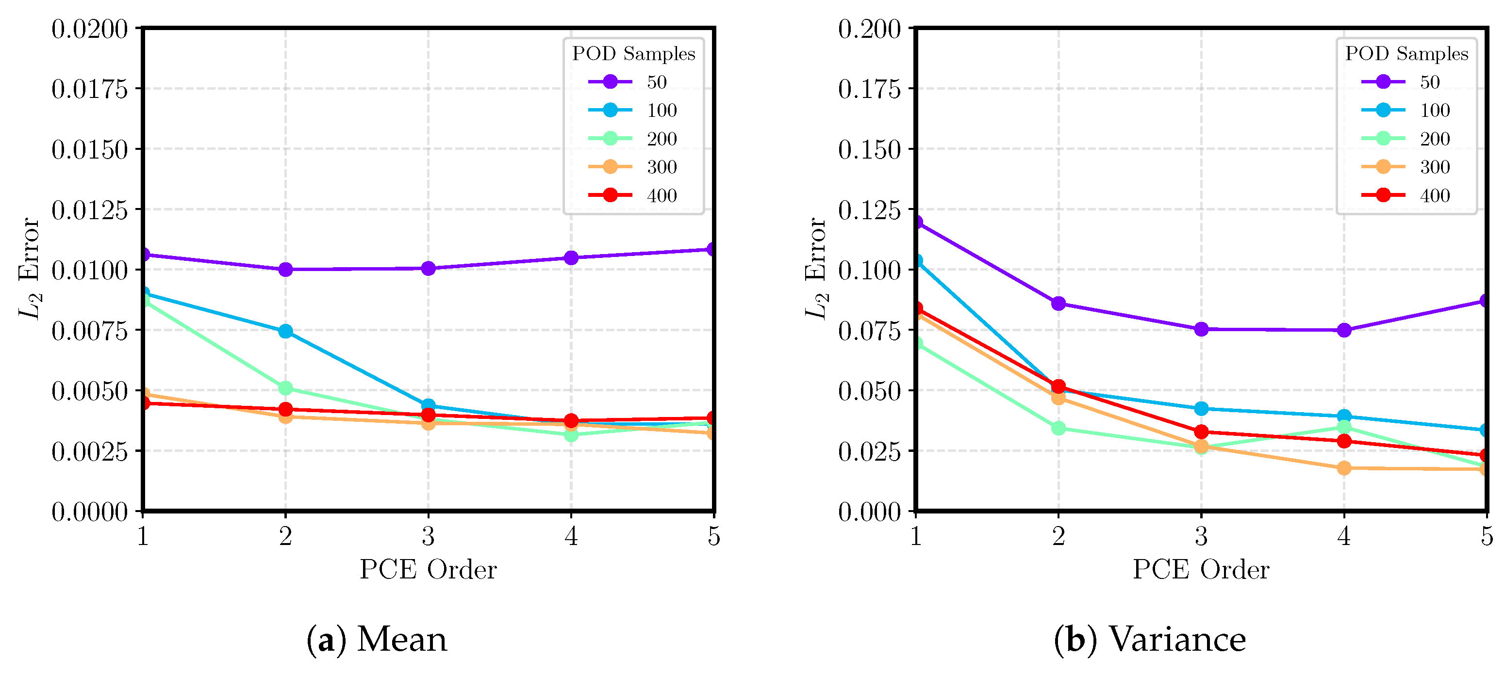
Figure 16 shows the impact of varying training samples and PCE order on the integrated error for the mean and variance. Overall, the mean response is predicted accurately, and performance improves marginally if PCE order increases and the uncertain PDFs are sampled more densely. For variance, there is a decrease in error with increasing samples and PCE order, but since RIC is fixed, all curves asymptote to nearly the same value as higher-order polynomials are used. Thus, if the variance or any higher-order statistic is to be better captured, the PCE order, the RIC, and the training sample size should all be increased.
It is essential to not only understand how well the models perform over the entire domain, but also to isolate their ability to reconstruct the variations of integrated quantities. As such,
Figure 17 shows the variation of the lift coefficient for the airfoil. It is seen that the ROM is able to accurately reconstruct the distribution. This indicates that lift coefficient can be predicted precisely even if the shockwaves in the flow are not.
4.3. Uncertain Supersonic Flow over Commercial Passenger Aircraft
The test case below assesses the performance of the methodology in predicting 3D uncertain supersonic flow over a supersonic transport aircraft (SST). While this test case also uses a CFD solver to obtain the snapshots, the number of nodes in the mesh is seven times larger compared to the airfoil test case. Moreover, since this is a fully 3D flow, there are strong interactions between components of the aircraft.
The geometry used is based on a notional 60-passenger SST designed for a cruise Mach number of 1.6 (see
Figure 18). The nacelle and tail were removed to simplify the computational domain and reduce convergence time. Uncertainty is introduced in the problem through two variations in the operating conditions: Specifically, the Mach number is normally distributed with a mean of 1.6 and a standard deviation of 0.05. The angle of attack is also normally distributed with a mean of
and a standard deviation of
. Together, these parameters change the flow over the entire aircraft by varying the shockwave structure and shape around the body. To resolve the flow, a computational mesh with 118 M nodes is created around the aircraft. Since the computational mesh is large, an inviscid analysis was executed with the compressible Euler equations. The Barth–Jespersen limiter [
25] is used for controlling numerical dissipation along with the flux-vector splitting approach of van Leer [
26]. An LHS DOE was used to obtain 300 training and 1500 validation snapshots.
Based on the results from the airfoil test case, only a fifth-order PCE model is used to fit the latent space since it is expected to be highly nonlinear. Given the large size of the computational domain, the ROM is fit only on the extracted surface data, which resulted in a snapshot having n = 77,500 nodes.
Figure 19 shows the solution predicted for one sample from the validation set. From the FOM solution, it is seen that the flow has a shockwave that occurs toward the wing tips and lacks discontinuities everywhere else in the domain. Thus, although the governing equations themselves are nonlinear PDEs, the solution is largely smooth other than at the wing tips. Unlike the airfoil test case, the inviscid analysis, combined with the variation of the uncertainties, results in flows where the Mach number is greater than one for all points on the surface. In agreement with the previously seen trends, the POD–PCE model performs well in the regions without shockwaves and is able to accurately reproduce the pressure distribution with little error. The Gibbs phenomenon is witnessed near the wing tips where an oscillatory error pattern exists. The region of error increases toward the trailing edge of the wing where the shockwave has greater variance, which causes an increase in the nonlinearity of the POD modes. Thus, the data suggest that if the flow is entirely supersonic (or subsonic) or if the shockwave’s variance is limited, then the POD–PCE method can predict the pressure distribution accurately.
For different Mach numbers and angles of attack, the intersection of the Mach cone with the wing leads to variations in the shock location. The aggregate performance of the models can be assessed using the RMSE, which
Figure 20 provides. Given that the POD–PCE model has shown error near the discontinuity, the RMSE has a large rise near the wing tips. The region of error increases downstream of the leading edge as the variations increase and oscillations rise. Away from the shock, the model has near-zero error and closely matches the FOM data.
Figure 21 shows the mean field over the aircraft surface and the componentwise relative error at each node. For POD–PCE, the mean is precise everywhere except near the wing leading edge. This results in an integrated error of
. The integrated error for variance is an order of magnitude larger compared to the mean error and equals
. As can be seen from the FOM plot in
Figure 22, there is a larger variation in the pressure values for the aircraft toward the leading edge, which results in a corresponding decrease in accuracy. Other than this isolated region of high error, at all other points, POD–PCE performs well and enables the rapid computation of moments.
5. Conclusions
The design of novel aircraft, especially those which deviate significantly from previous designs, is challenging due to the lack of historical data and high cost of experimental data acquisition. This challenge is further exacerbated by uncertainty during the manufacturing process, flight conditions, and atmospheric properties, which can cause significant changes to the aircraft performance. In some cases, the variations in performance can lead to program delays that increase overall cost.
While the methods used for reduced order modeling and accelerating uncertainty quantification are closely related, the two disciplines have largely operated in isolation until recently. This research provides a comprehensive characterization of the POD–PCE method, a parametric, non-intrusive, ROM-based strategy for accurately and efficiently predicting high-dimensional fields. Using three CFD-based test cases from quasi-1D internal flow to 2D flow over airfoils, to 3D flows over aircraft, a thorough assessment of the POD–PCE method is provided.
The findings show that, even with sparse datasets, the current methodology enables the efficient propagation of uncertainty in fields with shockwaves as the dimensionality is reduced by over two orders of magnitude. Specifically, it was observed that if the flow is entirely supersonic (or subsonic) or if discontinuities are limited to a small fraction of the overall computational domain, then the POD–PCE method can predict the pressure distribution accurately. However, near shocks, the above method has a sharp rise in error due to the inherent limitations of the PCE model in capturing the highly nonlinear variations of POD modes.
The POD–PCE method is limited by the effectiveness of the UQ model in the latent space. In fact, the regression error contributes to over 75% of the total error in some cases and reflects the challenges of capturing the dynamics of the latent space. The RMSE, and the error of the variance field, are near zero throughout the domain except near the vicinity of the shockwaves. However, as the PCE regression order and training sample size are increased, the models become increasingly more accurate, albeit less parsimonious.
Together, these findings further support the hypothesis that the proposed method performs well in simulations seen in subsonic aircraft design. In the future, the use of alternative dimensionality reduction methods, such as those that rely on manifold learning to identify a nonlinear latent space, will be explored. It is hypothesized that nonlinear DR methods may alleviate the challenges of approximating shocks and therefore reduce error. Future studies will also investigate extensions to PCE models, such as multi-element and kernel-based approaches, to improve latent space regression.


