1. Introduction
The exploration of Venus has captivated scientists and space enthusiasts since the beginning of the space age. In 1962, the Mariner II probe performed a close flyby of Venus, collecting crucial atmospheric data and marking the first successful interplanetary mission [
1,
2]. Following this, the Venera program accomplished noteworthy achievements, including the first impact on another celestial body (Venera 3, 1965) and successful atmospheric entry (Venera 4, 1967). Subsequently, the program achieved data transmission (Venera 7, 1970) and imagery capture (Venera 9, 1975) from the surface of Venus [
3,
4]. These early missions were primarily dedicated to the landing of probes on the Venusian surface, and it took 13 years after Mariner II for the deployment of the first orbiter, Venera 9.
Starting from the late 70’s and through the 80’s, the interest in comprehending Venus’s surface and atmosphere prompted the development of orbiters. Data from the Pioneer Venus 1–2 spacecraft (1978) allowed producing the first topographical map of Venus surface and provided atmospheric data within an altitude range of 10 to 50 km [
5]. These results were later improved by Magellan (1989), offering a high-resolution synthetic aperture radar map of the Venusian surface with details down to 120 and 300 m [
6]. Furthermore, Venus Express (2005) generated a temperature map of the planet’s southern hemisphere and collected information to study the upper atmosphere [
7].
To date, the only spacecraft orbiting Venus is Akatsuki (2010), operated by JAXA, dedicated to investigate Venus’s climate. However, a renewed interest in the planet’s evolution and human space exploration is leading the design of novel mission architectures [
8,
9,
10,
11]. In this context, Haibin et al. explored the feasibility of fast low-energy halo-to-halo transfers to reduce fuel consumption and flight time with respect to traditional solutions [
12]. Zubko et al. proposed the use of resonant orbits to expand landing areas and ensure landing in the desired region [
13,
14]. This approach could even be extended to transfer an orbiter from Earth to Venus using a free-impulse flyby of an asteroid [
15]. Heiligers et al. studied the application of solar sails to maintain pole-sitters at Venus, enabling continuous planetary polar observation [
16]. Girija et al. expanded the use of aerocapture at Venus, demonstrating its effectiveness in deploying satellites in low-altitude circular orbits with different inclinations [
17]. The problem of rideshare launches to Venus was also addressed by Graham et al., who combined patched perturbed Sims–Flanagan trajectories and low-thrust propulsion to design an Earth-Venus trajectory which concludes in a weak capture around the arrival planet [
18]. Additionally, in the broader context of space exploration, the choice of a nominal space telescope orbit around the Sun-Venus L2 libration point has been discussed by Shirobokov et al., emphasizing its appeal for observing potentially hazardous asteroids approaching Earth from the daytime side of the sky [
19].
In this work, we develop an Earth-Venus mission which leverages the use of traditional high-energy interplanetary transfers, low-energy captures and nonlinear orbit control for low-thrust propulsion to inject a spacecraft into any desired orbit at Venus. Low-energy trajectories are special solutions of the restricted 3-body problem, whose applications were extensively investigated in the past decades [
20,
21,
22,
23,
24,
25]. Their use in the design of an Earth-Venus transfer, though attractive because it leads to savings in the total delta-V (propellant mass) required [
26,
27], has a major drawback in the longer transfer time. The combined use of high- and low-energy trajectory, developed here, allows preserving the saving in propellant mass while limiting the increase in the transit time [
28]. Nonlinear orbit control, implemented through an original feedback control law, and low-thrust propulsion allow maneuvering the spacecraft from the capture orbit to the target one [
29].Two target orbits, originally selected for the Venus Flagship Mission by the Goddard Space Flight Center, are considered in this study: (i) an elliptic orbit with semilatus rectum of 12,075.7 km, eccentricity of 0.9011 and inclination of 90
, and (ii) a circular orbit with the same inclination and altitude of 300 km [
30].
The paper is organized as follows. The mathematical model of the dynamical frameworks are presented in
Section 2. Nonlinear orbit control is developed in
Section 3.
Section 4 provides an overview of the mission profile and a description of the Earth-Venus interplanetary arc. The low-energy capture at Venus and the orbit injection are discussed in
Section 5, including also applications on the above-mentioned test cases. Final remarks are reported in
Section 6.
3. Nonlinear Orbit Control
We present a nonlinear feedback orbit control law for the guidance of a spacecraft toward some desired conditions. These are specified in terms of modified equinoctial elements, as a function of
only, in the following target set:
where
is a nonlinear vector function, such that
(at most one condition can be imposed for each orbital element contained in
).
The feedback control law is constructed using the direct method of Lyapunov, which provides sufficient conditions for stability and avoids linearization around a reference solution [
44]. The following candidate Lyapunov function is introduced:
where
is a diagonal matrix with positive constant elements (representing weight coefficients selected a priori based on the application) and it is positive definite. It is easily recognized that
, with
if and only if
(i.e., if the target state is reached), making it a definite positive function. Additional conditions must be satisfied for
V to be a valid Lyapunov function. First, we introduce the following auxiliary vector:
Two propositions establish the conditions for V to serve as a Lyapunov function and lead to the identification of a saturated feedback law.
Proposition 1. If ψ and are continuous, unless , and , then the feedback control lawleads a dynamical system governed by Equations (4) and (7) to converge asymptotically to the target set associated with Equation (20). Indeed, the proposed control law ensures that
with
, which corresponds to the attracting set. Therefore, it establishes the candidate function (
21) as a valid Lyapunov function [
44]. As a result, the control law (
23) drives the dynamical system to asymptotically converge to the target state defined by (
20). This control law incorporates feedback from the spacecraft state in all its terms, except for the weight matrix. By leveraging the information provided by the state variables, the control law dynamically adjusts the direction and magnitude of thrust at each iteration, enabling the achievement of the desired orbital conditions. However, the physical feasibility of the control lies in ensuring that the magnitude of
does not exceed
. Consequently, the condition
must be satisfied to ensure control feasibility. In cases where this constraint is violated, an alternative feedback control law can be employed, which operates in a saturated manner by applying maximum thrust.
Proposition 2. If ψ and are continuous, unless , and and , then the feedback control lawleads a dynamical system governed by Equations (4) and (7) to converge asymptotically to the target set associated with Equation (20). It can be shown that for the given control law,
if
, while no conclusions can be drawn if
[
45]. The sign of this term generally varies over time and relies on the specific time-evolution of the dynamical system. Consequently, an additional sufficient condition is necessary to ensure that
even when
.
Proposition 3. If ψ and are continuous, unless , and , then the feedback control law in Equation (24) leads a dynamical system governed by Equations (4) and (7) to converge asymptotically to the target set associated with Equation (20). Proposition 3 provides a valuable sufficient condition with a clear interpretation: if the magnitude of the thrust acceleration, , exceeds the perturbation acceleration magnitude, , then unless .
The two feedback laws presented in Equations (
23) and (
24) can be combined into a single expression:
This control law can be implemented using steerable and throttleable propulsive thrust, where both the magnitude and direction can vary over time.
Propositions 1–3 establish sufficient conditions for Lyapunov stability. Consequently, the asymptotic convergence is not necessarily compromised if becomes positive within limited time intervals.
Nonlinear Control for Semi-Major Axis, Eccentricity, and Inclination
With the newly defined control law, we aim to achieve a specific target state identified by the following orbit elements: semi-major axis, eccentricity, and inclination. This implies that the other orbital elements are left free and can take any value within their respective ranges. The desired conditions, denoted with the subscript
d, can be expressed by the following equations:
where
and
. We define the vector that represents the target set as:
We analytically derive the components
of the vector
to be used in the control law (
25):
where
represent the elements of the diagonal matrix
.
We proceed with the identification of the attracting set, collecting all the dynamical states that satisfy . This set includes the target set since implies . However, the reverse is not guaranteed. As a matter of fact, considering the definition of , it includes the term among its factors: if this term is zero, then . However, it is possible for to cancel out due to other terms. This implies that but , resulting in the non-attainment of the target state. Hence, it is possible to reach the attracting set without reaching the target set (, ), leading to the settling of the Lyapunov function at a nonzero steady-state value, thereby achieving a different condition than the desired target.
In our case, the attracting set includes the following subsets [
46]:
- 1.
(rectilinear trajectories);
- 2.
, , and (equatorial elliptical orbits with semilatus rectum and eccentricity );
- 3.
, , and (circular orbits with radius and inclination );
- 4.
, , and (circular equatorial orbits with radius );
- 5.
, , and (target set).
The application of LaSalle’s invariance principle allows ruling out subset 1.
Given the continuity of
and
(except within the attracting set, denoted as
A), the condition
, where
represents the evaluation of
at the initial time, defines a compact set
C. To apply LaSalle’s principle, we seek the invariant set within the intersection of
A and
C. The invariant set comprises dynamical states within the attracting set of
that remain unchanged when
. Consequently, once the invariant set is reached,
at subsequent times, implying
while
. In this specific scenario, when
, the time derivatives of the three components of
can be expressed as
An examination of
reveals that subset 1 (
) does not belong to the invariant set, thereby ruling out convergence toward rectilinear trajectories. On the other hand, subsets 2 and 5 constitute the invariant set for the given problem [
46].
It should be noted that convergence toward subsets 2 through 5 is purely theoretical, as demonstrated in [
46], with the interesting practical consequence that the dynamical system under consideration exhibits global convergence toward the desired operational conditions when the control law (
25) is adopted.
4. Interplanetary Transfer
The mission begins at the satellite deployment on a Trans-Lunar Injection (TLI) trajectory, chosen to be compatible with currently available rideshare opportunities, with orbit parameters summarized in
Table 1. Depending on mission requirements, the orbital inclination can be either 57
or the supplementary 123
(retrograde launch), while the right ascension of the ascending node and the argument of perigee can be freely chosen.
After being released from the launcher, the spacecraft undergoes a first three-dimensional impulsive maneuver at the apogee to increase its energy and adjust the inclination, which is necessary for the spacecraft to be on the right trajectory toward Venus. The perigee altitude is raised to 1000 km, a value chosen to minimize the energy losses by thrusting as close as possible to the attracting body (Earth) [
34], while avoiding crossing the Low Earth Orbit region. The selection of 1000 km, although arbitrary, appears reasonable and serves as a mission constraint. Subsequently, at the perigee, another critical impulsive maneuver called Trans-Venus Injection (TVI) is executed. With this maneuver, the spacecraft is transferred to a hyperbolic orbit, reaching Venus at a pericenter altitude of 300 km. Upon reaching Venus, the mission explores two distinct scenarios to achieve capture around the planet and the attainment of the target orbits, with the goal of minimizing the total propellant usage:
- 1.
The first scenario, named “APO”, achieves this objective by first targeting a specific “optimal apocenter” altitude for the initial capture around Venus and then employing nonlinear low-thrust control to reach the desired target orbit.
- 2.
The second scenario, labelled as “L1”, focuses on the use of low-energy captures designed in the equilibrium region about .
These scenarios will be comprehensively discussed in
Section 5.
The preliminary interplanetary trajectory from Earth to Venus is designed using the patched conics method, which simplifies calculations in a multi-body environment while ensuring accuracy [
34]. This method divides the trajectory into three arcs: a hyperbolic departure trajectory from Earth, an elliptical heliocentric transfer arc, and a hyperbolic arrival trajectory to Venus. The first and third arcs are considered within the sphere of influence of the respective planet, with the Sun acting as the only attracting body beyond these regions in the second arc. To determine the velocities at departure and arrival, the hyperbolic excess velocities
and
are calculated.
represents the excess velocity at departure relative to Earth, while
corresponds to the velocity at arrival at Venus. These velocities are obtained by subtracting the velocities of Earth and Venus from the departing and arriving velocities in the heliocentric frame, respectively. Specifically, we have:
Here, and represent the departing and arriving velocities, while and denote the velocities of Earth and Venus, respectively.
The mission timeline is set between 2029 and 2033, aligning with the launch periods of notable future missions such as VERITAS, EnVision, DAVINCI+, Venera-D, and the Venus Flagship Mission [
10,
47,
48,
49,
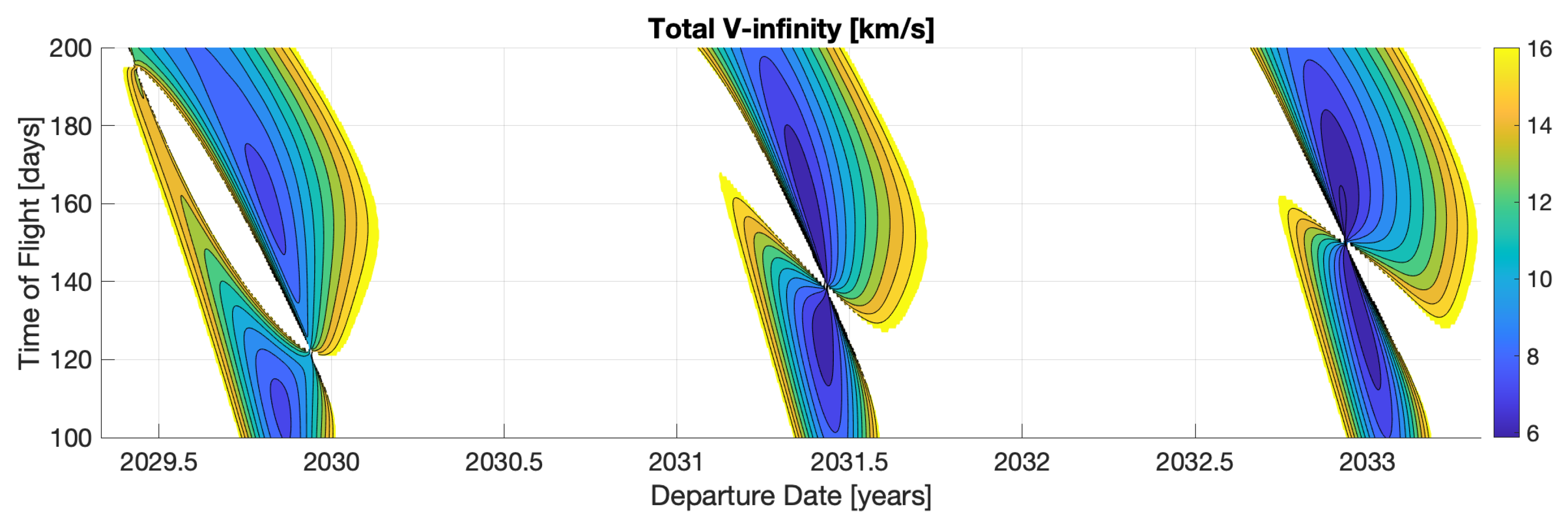
50]. To analyze the optimal launch opportunities, porkchop plots are generated for the years 2029–2033, covering each day of the year with a flight duration (ToF, Time of Flight) ranging from 100 to 200 days. This range for the ToF is chosen based on the consideration of a “short” journey to Venus, although more fuel efficient longer duration solutions may exist. By examining the results of the porkchop plots, launch opportunities that align with the available propulsion capabilities can be identified. These plots depict contour lines of the hyperbolic excess velocity (
) in relation to combinations of departure and arrival dates. They are generated by solving the Lambert’s problem for all possible combinations of departure and arrival dates within specified intervals. The algorithm outputs the initial and final velocities of the spacecraft,
and
, along the transfer heliocentric trajectory. Then the two hyperbolic excess velocities (
and
) are calculated using Equations (
32) and (
33). The DE405 ephemerides are used for the positions and velocities of the two planets.
To systematically search for the optimal heliocentric transfer, the sum of the hyperbolic excess velocities is minimized:
The desired solution corresponds to the best combination of departure date and corresponding time of flight which minimizes . This overall minimization reduces the propulsion effort required for departure from Earth and orbital insertion around Venus, resulting in propellant savings.
An exhaustive investigation is conducted to find the minimum value of
, with the porkchop plots generated using MATLAB. The obtained solution is presented in
Table 2.
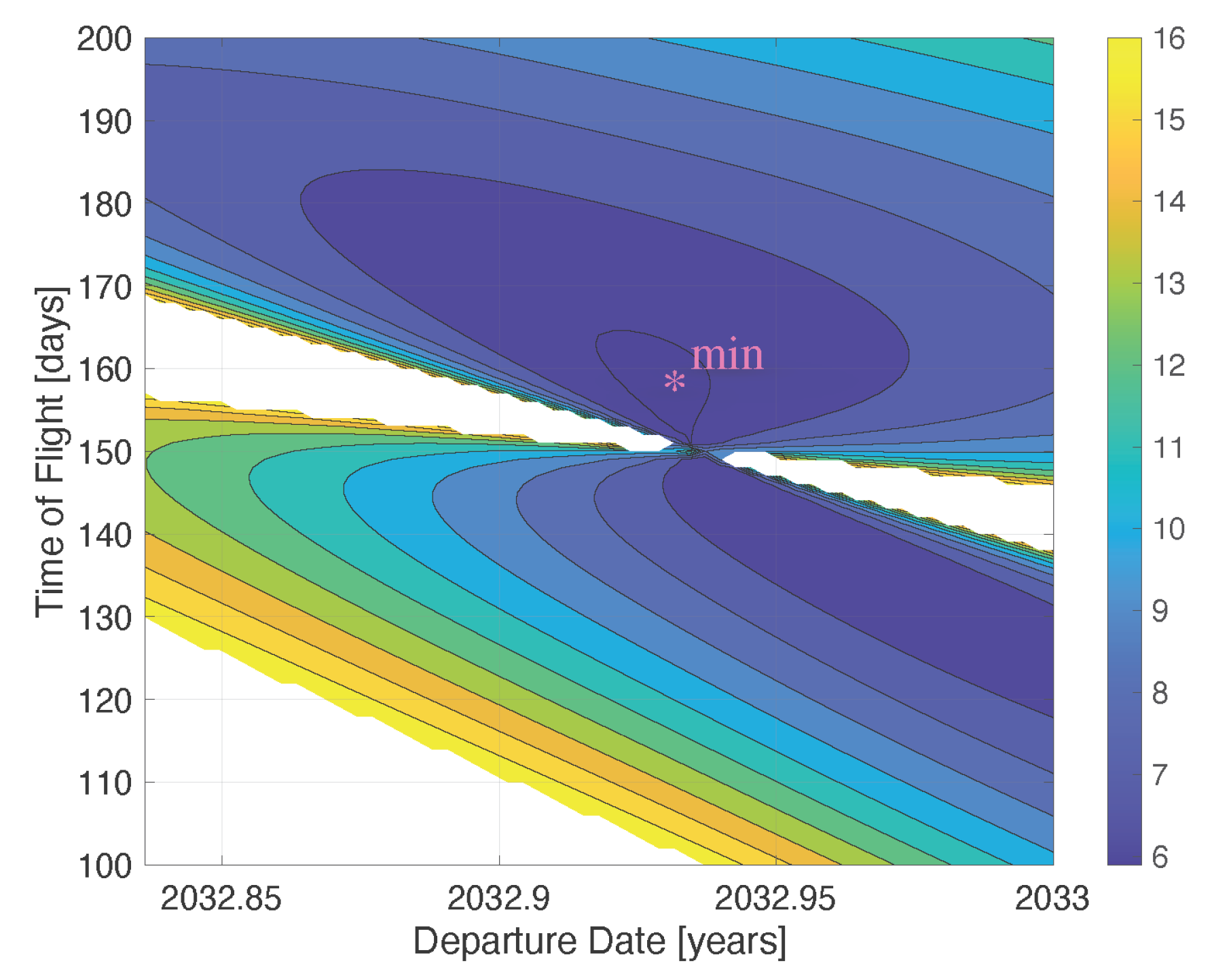
The porkchop plots, displayed in
Figure 2 and
Figure 3, provide a visual representation of the transfer options for the years 2029 to 2033, with a specific focus on 2032. The optimal solution corresponds to a departure on 6 December 2032, and an arrival 158 days later on 13 May 2033. The resulting
is calculated as
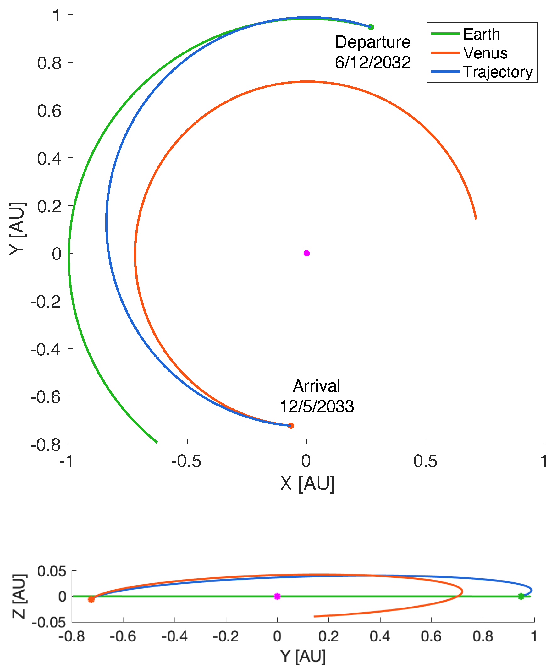
km/s. Notably, this solution is located in the same region as the minimum arrival hyperbolic excess velocity at Venus, rather than the departure from Earth. The trajectory corresponding to this optimal solution, obtained using the Lambert problem solver algorithm, is depicted in
Figure 4. This trajectory serves as the baseline for the mission and is reproduced using the General Mission Analysis Tool (GMAT) propagator [
51], in a high-fidelity framework.
During our investigation, we explored alternative trajectories and discovered a more advantageous solution that involved multiple revolutions. This alternative solution, with a departure on 5 June 2032, and arrival on 31 August 2033, resulted in a total
of 5.6163 km/s. Compared to the previously identified optimal solution, this alternative solution offered a reduction of 280 m/s in total
, but at the expense of a 452-day travel duration, nearly three times longer.
Table 3 presents the main parameters of the Hohmann transfer for reference, which can serve only as a comparative case (because it assumes coplanar circular orbits of Earth and Venus). Taking into account the trade-off between energy savings and extended travel durations, we selected the shorter optimal solution as the reference for our mission.
The initial reference solution involves departing from Earth on 6 December 2032, at 05:00 UTC, and arriving at Venus on 12 May 2033, at 17:00 UTC. It’s important to note that these dates do not consider the dynamics inside the spheres of influence or perturbations. In the following sections, we will address these factors by employing GMAT for the propagation.
The mission profile outlined at the beginning of
Section 4 is designed using backward propagation, from the Venus arrival date, which allows for a more detailed specification of arrival conditions and enhances flexibility during the Earth departure phase. The spacecraft’s arrival at Venus is set to 12 May 2033, at 17:00 UTC. The trajectory is hyperbolic, characterized by a pericenter altitude of 300 km and an excess velocity
km/s (
km
/s
), as determined from the porkchop plots. By employing a Target sequence in GMAT, the orientation of the hyperbola at Venus is determined, enabling backward propagation to achieve an Earth return with an altitude of 1000 km from the hyperbolic perigee. The dynamical model for this phase includes the Sun, Venus, Earth, and the Moon as point masses, while disregarding other perturbations. It is worth noting that multiple combinations of parameters exist that yield the same
, resulting in hyperbolas that share energy and asymptote direction. To further optimize the mission, additional conditions can be imposed, such as matching the initial inclination to the one of the TLI trajectory, thereby eliminating the need for costly plane change maneuvers.
In the APO strategy, the spacecraft is transferred to the TVI trajectory on 5 December 2032, at 14:40 UTC, which is approximately 14 h earlier than the solution derived from the porkchop plots. This indicates that the solution obtained in GMAT, which considers accurate propagation, deviates by less than a day compared to the Lambert algorithm. Moreover, the obtained in GMAT is 3.1651 km/s, closely matching the reference value of 3.1757 km/s, with a difference of approximately 11 m/s. These results can be considered satisfactory.
On the other hand, the L1 strategy requires one or more deep space maneuvers (DSMs), within the interplanetary arc, to adjust the angles
of the arrival hyperbolic trajectory at Venus so that the spacecraft can be later injected into the equilibrium region about
, as detailed in
Section 5.2. To determine the necessary DSM, a new Target sequence is created in GMAT, focusing on finding the maneuver components in the Vertical-Normal-Binormal (VNB) reference frame [
51]. This DSM, like the other maneuvers, is considered impulsive. In interplanetary missions, corrective maneuvers typically involve modest impulses of tens of m/s. Analytical studies have shown that applying an infinitesimal impulse at an infinite distance from the attracting body can modify the eccentricity of a hyperbolic trajectory without changing its energy [
53]. This insight is valuable as it allows for the adjustment of the pericenter radius through small impulses at significant distances, without introducing substantial energy variations to the trajectory.
In this particular case, a single corrective impulse, represented as
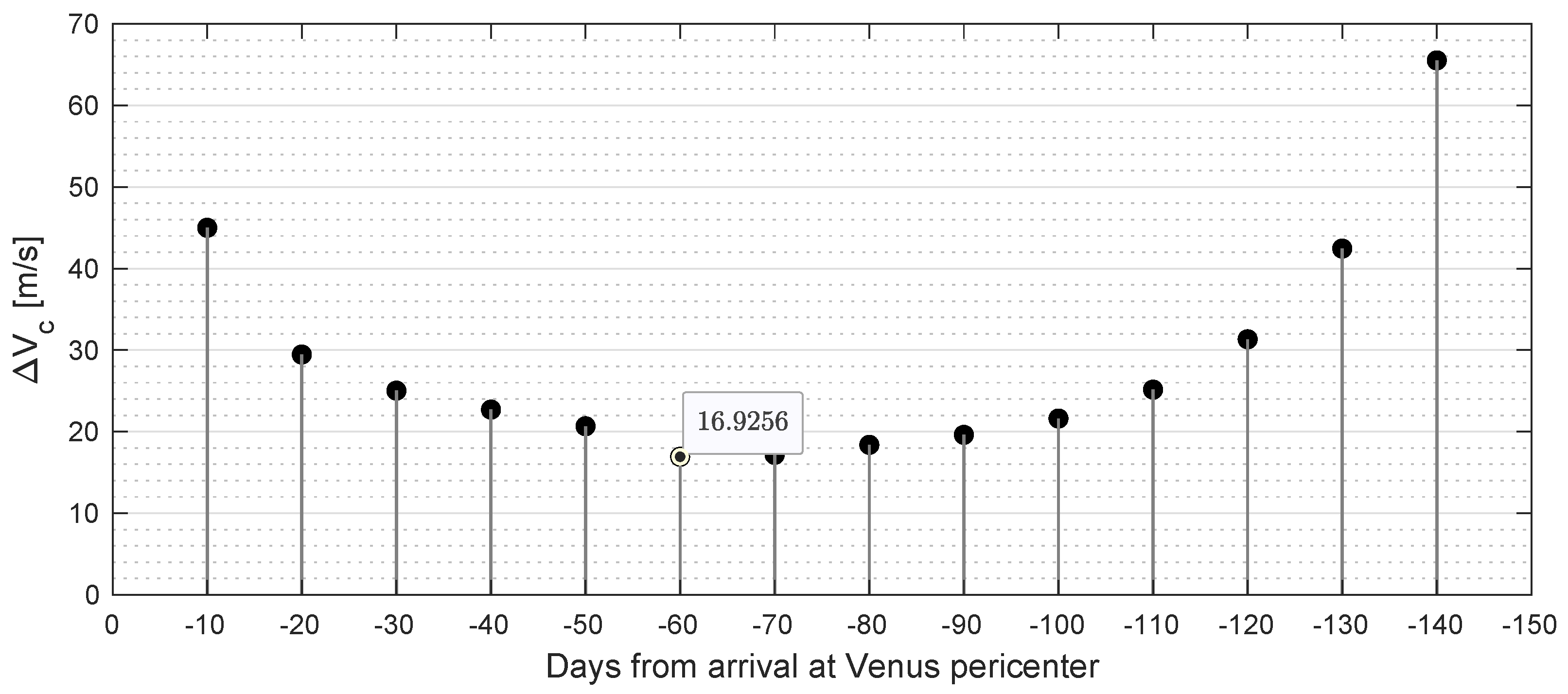
, is sufficient. The timing of the maneuver is a parameter that can be adjusted to minimize the magnitude of the delta-v and reduce propellant consumption. By iteratively modifying the application position in GMAT and calculating the corresponding delta-v magnitude, it is possible to approximate the region where the minimum occurs.
Figure 5 provides a visualization of some of these results. The magnitude of the corrective delta-v is plotted as a function of the days before arrival at Venus pericenter. The results indicate a decreasing trend until reaching a minimum value at approximately 60 days prior to arrival (
m/s at −60 days). Beyond this point, the magnitude of the delta-v starts to increase.
Further investigation leads to the determination of the optimal solution. Utilizing the Yukon optimizer, a slightly different solution is obtained with a delta-v magnitude of 16.8 m/s at −59.98 days. This final solution, achieved by adjusting the corrective impulse, ensures an inclination close to 123
at the perigee, enabling the utilization of the retrograde TLI trajectory. The components of the corrective impulse are listed in
Table 4.
Finally, for both the APO and L1 strategies, the angles
that identify the orientation of the hyperbola are presented in
Table 5 in the VCI frame.
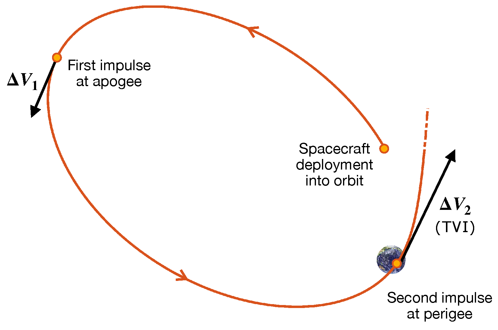
4.1. Impulsive Maneuvers in the Geocentric Arc and Propellant Consumption Analysis
Two maneuvers are performed in Earth’s orbit to transition from the Trans-Lunar Injection trajectory (specified in
Table 1) to a hyperbolic departure from Earth. The first maneuver,
, occurs at apogee and aims to increase the radius at perigee. It is typically a three-dimensional maneuver, with an out-of-plane correction if necessary. The second maneuver,
, takes place at perigee and is executed along the velocity vector to enter the desired hyperbolic orbit with a perigee altitude of 1000 km.
Figure 6 depicts a representation of this phase, starting from the spacecraft’s orbital insertion after launch.
According to Kepler’s theory, the
value can be calculated as
In the above equation, the subscript
P denotes the perigee, while the subscripts + and − represent the values after and before the maneuver. This value serves as a reference for refinement in GMAT, where the dynamic model incorporates Earth’s gravitational contribution, considering spherical harmonics up to the 4th degree and order, as well as perturbations from the Sun and Moon.
Using GMAT, the magnitude of
is determined to be
m/s. The individual components in the VNB reference frame are reported in
Table 6.
The magnitude of obtained through GMAT’s Target sequence is very close to the predicted value, measuring m/s. The overall delta-v budget in Earth’s orbit, , is the sum of and , amounting to m/s.
To estimate the propellant required for these maneuvers, we apply the Tsiolkovsky equation with an effective exhaust velocity of m/s. This allows us to calculate the mass ratio , representing the final mass () of the spacecraft after all maneuvers, relative to its initial mass (). After applying the equation to the total delta-v, , we find a final mass ratio of or , indicating that only of the propellant has been consumed compared to the probe’s initial mass.
For the L1 strategy, the magnitude of the delta-v values are
m/s (at apogee) and
m/s (at perigee), respectively. The components of
in the VNB reference frame are detailed in
Table 6. In this case, the total delta-v in Earth’s orbit,
, includes the two delta-v values in the geocentric arc and the corrective delta-v. The sum is
m/s. The final mass ratio is determined to be
or
, indicating a propellant consumption of
before entering Venus’s sphere of influence.
4.2. Comparative Analysis of Mission Profiles
It is beneficial to compare the two mission profiles designed so far.
For the “APO” scenarios, the trajectory follows the following sequence:
- 1.
Launch and insertion into a direct TLI trajectory on November 24, 2032, at 1:03 UTC.
- 2.
Application of a three-dimensional impulsive maneuver at apogee to lower the pericenter altitude and slightly change the inclination (magnitude of 7.7 m/s).
- 3.
Application of an impulsive maneuver at perigee in the direction of velocity for insertion into the departure hyperbola (magnitude of 560 m/s).
- 4.
Ballistic interplanetary arc until arrival at Venus with a pericenter altitude of 300 km and a velocity of 10.473 km/s.
For the “L1” scenario, the sequence presents some differences:
- 1.
Launch and insertion into a retrograde TLI trajectory on 23 November 2032, at 21:17 UTC.
- 2.
Application of a three-dimensional impulsive maneuver at apogee to lower the pericenter altitude and slightly change the inclination (magnitude of 24.9 m/s).
- 3.
Application of an impulsive maneuver at perigee in the direction of velocity for insertion into the departure hyperbola (magnitude of 565.6 m/s).
- 4.
Interplanetary arc with an intermediate corrective impulse (magnitude of 16.8 m/s).
- 5.
Arrival at Venus with a pericenter altitude of 300 km and corresponding velocity of 10.473 km/s.
5. Capture and Orbit Injection at Venus
Upon reaching the 300 km pericenter along the hyperbolic orbit on 12 May 2033, at 17:00, the spacecraft can employ various strategies to achieve the desired orbits around Venus. In the subsequent paragraphs, we present comprehensive descriptions of these strategies for both target orbits. Each scenario involves a Venus Orbit Insertion (VOI) maneuver at the pericenter to decelerate the spacecraft, with the magnitude of deceleration tailored to the specific strategy. Chemical propulsion is employed for the high-thrust phase, while electric propulsion is used for the low-thrust phase, following the control law (
25) to achieve the target orbit parameters, including semi-latus rectum, eccentricity, and inclination. The performance parameters for the low-thrust system are:
Here,
represents the effective exhaust velocity for low-thrust propulsion (LT), and
represents the maximum thrust acceleration relative to the spacecraft’s initial mass (
) at launch. The values selected are of the same order of magnitude as those of Busek BIT-3 ion thrusters [
54]. To consider the maximum propulsive acceleration relative to the initial mass
during the low-thrust control phase, normalization of
by the corresponding mass ratio
is necessary.
5.1. Capture in Highly Elliptic Orbit and Low-Thrust Orbit Injection
The first scenario (named “APO”) involves the impulsive application of the VOI maneuver at the pericenter of the inbound hyperbolic trajectory toward Venus, followed by a low-thrust orbital control phase. The VOI maneuver, performed using chemical propulsion in the opposite direction of the spacecraft’s velocity, reduces the spacecraft’s energy and inserts it into an elliptical capture orbit around Venus.
For this scenario, three different strategies are considered, indicated as “APO.A,” “APO.B,” and “APO.C.” Each strategy is analyzed twice: for the final elliptical orbit and for the final circular orbit. The magnitude of the impulsive delta-v at the pericenter associated to the VOI, denoted as
, varies case by case based on the strategy and the target orbit. It is optimized to minimize the overall propellant consumption, considering both chemical and electric propulsion. Depending on the magnitude of
, the spacecraft is inserted into an elliptical orbit with varying eccentricities (same pericenter radius and different apocenter radii). Increasing the magnitude of
reduces the apocenter radius of the elliptical orbit, while decreasing the impulsive maneuver intensity results in a more energetic elliptical orbit with a higher apocenter altitude. At first glance, the latter case may seem more advantageous as it allows for initial propellant savings followed by the low-thrust phase. However, due to the non-linearity of the control law, reducing
does not necessarily reduce the overall propellant consumption since the low-thrust phase may require higher consumption. If it were the case, the minimum value of
would be sought, which would subsequently allow for the successful application of the non-linear low-thrust control. This delta-v might not be the minimum for inserting into an elliptical orbit, which means reducing the velocity just below the escape velocity. In fact, Equation (
25) can work in some cases even when applied to a hyperbolic orbit if the available thrust levels are sufficient [
55]. Since the intensity of the impulsive maneuver cannot be determined in advance, the value of
is sought to maximize the resulting mass ratio once the target orbit is reached.
To conduct this search, the insertion into an elliptical orbit with apocenter radius equal to the radius of Venus’s Sphere of Influence (SOI) is taken as a reference:
km (using the Laplace definition). A very high apocenter allows for significant savings in maneuver costs. The corresponding delta-v, denoted as
, is calculated using Keplerian theory:
where
represents the velocity at the pericenter before the maneuver (on the hyperbola), and
the velocity just after the maneuver (on the ellipse). The pericenter radius is calculated as:
, with
km [
56]. The result in (
36) is confirmed in GMAT.
The optimization process involves searching for the optimal value of in the vicinity of . Once the maneuver is applied, the low-thrust orbital control phase begins, aiming to reach the two target orbits using different strategies for each. The numerical iteration proceeds as follows:
This iterative process is repeated for a series of values to determine the one that maximizes the final mass ratio.
For each control gain, namely , , and , an initial range is manually defined. These intervals serve as a starting point for the Particle Swarm Optimization (PSO) process. Within these ranges, the particles in the swarm can explore and move. The results obtained from PSO can be further refined by using MATLAB’s fminsearch routine. The optimization of weights is performed for each strategy using a reference case that applies , and then these optimized weights are used for all considered values.
Since the exact time required to reach the target state is unknown in advance, the propagation is initiated for a predetermined number of days considered sufficient to achieve the objective. If needed, the propagation can be restarted for a longer duration. A stopping condition is also implemented: the numerical integration is halted when
, which implies
, related to MATLAB’s machine precision [
57]. When the weights are well-optimized, this condition is easily met. However, if the weights are not fully optimized, the propagation continues for the entire planned duration. It is important to note that even if the stopping condition is not met, it does not necessarily mean that the target conditions (such as obtaining
) are not reached. It simply suggests that the used weights may not be fully optimized yet.
In our study, we explore various cases based on the moment of ignition for electric propulsion, referred to as APO.A, APO.B, and APO.C strategies. These strategies aim to achieve the target orbit with the highest possible mass ratio while considering realistic mission scenarios and limitations.
The APO.A strategy assumes the immediate activation of low-thrust nonlinear control right after the application of . By initiating propulsion effects starting from the pericenter, this strategy allows us to analyze the impact of thrust on the trajectory. However, it is important to note that APO.A is not practically implementable as it assumes an instantaneous application of the VOI maneuver and immediate activation of the electric thruster right after.
In order to introduce more realism, the APO.B strategy incorporates a time delay of one hour between the impulsive application of and the activation of low-thrust control. This delay simulates the scenario where spacecraft state control can be performed and the two maneuvers can be temporally separated.
For the APO.C strategy, the low-thrust control is applied after propagating the spacecraft for an entire orbit until reaching the new pericenter. This approach ensures that the pericenter does not end up inside the planet with a negative altitude, which can be caused by significant third-body perturbations. In fact, solutions that result in a return to Venus with an altitude lower than 200 km are disregarded, as atmospheric perturbations become highly significant and potentially destructive.
The analysis begins with the examination of the elliptical target orbit with dimensions
km. The desired orbital parameters expressed in the VCI reference frame are:
The comprehensive results for all strategies and target orbits can be found in
Table 7, which provides the final mass ratio and the associated time of flight during the low-thrust control phase.
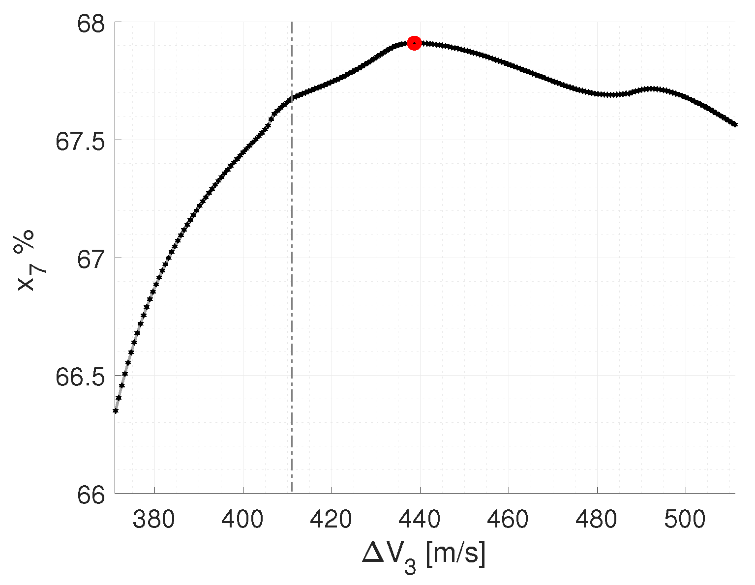
For the APO strategies, each time a range for
is explored for the optimization. For example, for APO.A,
is analyzed. The results of this analysis, with the
interval discretized into 200 points, are depicted in
Figure 7.
The maximum final mass ratio achieved is 67.91%, corresponding to
= 438.7 m/s. The reference
position, corresponding to a final mass ratio of 67.68%, is marked by a gray dashed vertical line. Further optimization in the vicinity of this solution leads to convergence to the target state after 17.77 days with a final mass ratio of 68.05%. Instantaneously applying
438.7 m/s corresponds to
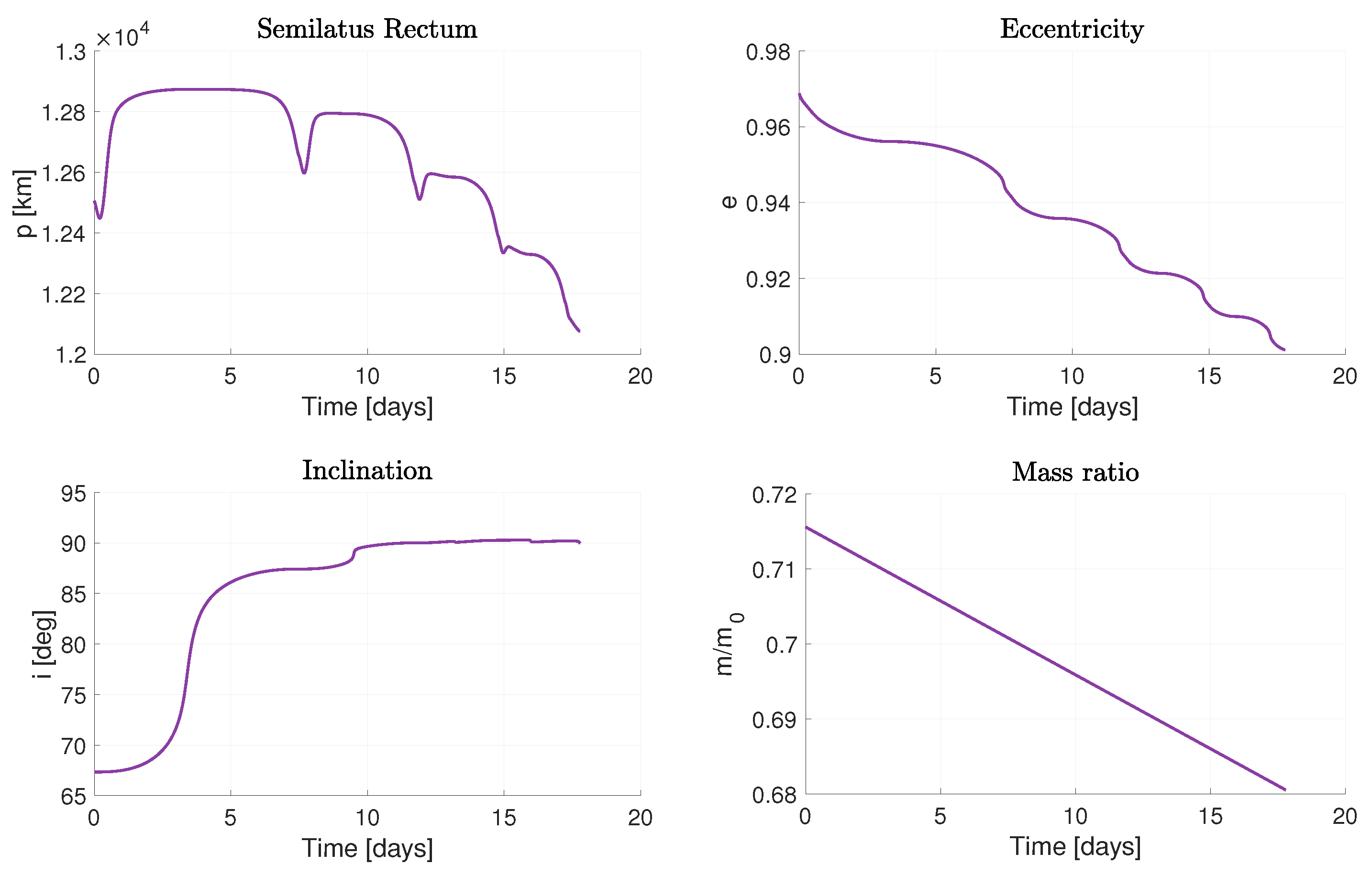
400,384.4 km. However, due to the gravitational effect of the Sun perturbing the trajectory, propagating to the apocenter yields a radius of 396,877.6 km. The temporal behaviors of controlled orbital parameters and the mass ratio are shown in
Figure 8.
By propagating beyond the necessary time to reach the target state, a change in the slope of the mass ratio can be observed. The absolute value of the slope decreases as the orbit tracking phase is completed, and the maintenance phase begins to compensate the gravitational effects related to spherical harmonics and the third body. For instance, by maintaining control for an entire year, the mass ratio decreases to 67.03%, resulting in an approximate 1% of mass depletion.
Similar results are obtained for the APO.B and APO.C strategies. The most favorable solution is provided by the APO.C strategy, with a higher final mass ratio of 68.12%. It also corresponds to the shortest time of flight, approximately 10 days.
The objective now is to achieve a circular orbit with an altitude of 300 km. The same principles discussed for the elliptical target orbit apply here as well. The desired orbital elements in the VCI reference frame are:
The three strategies are investigated again to minimize propellant consumption. The results are presented in
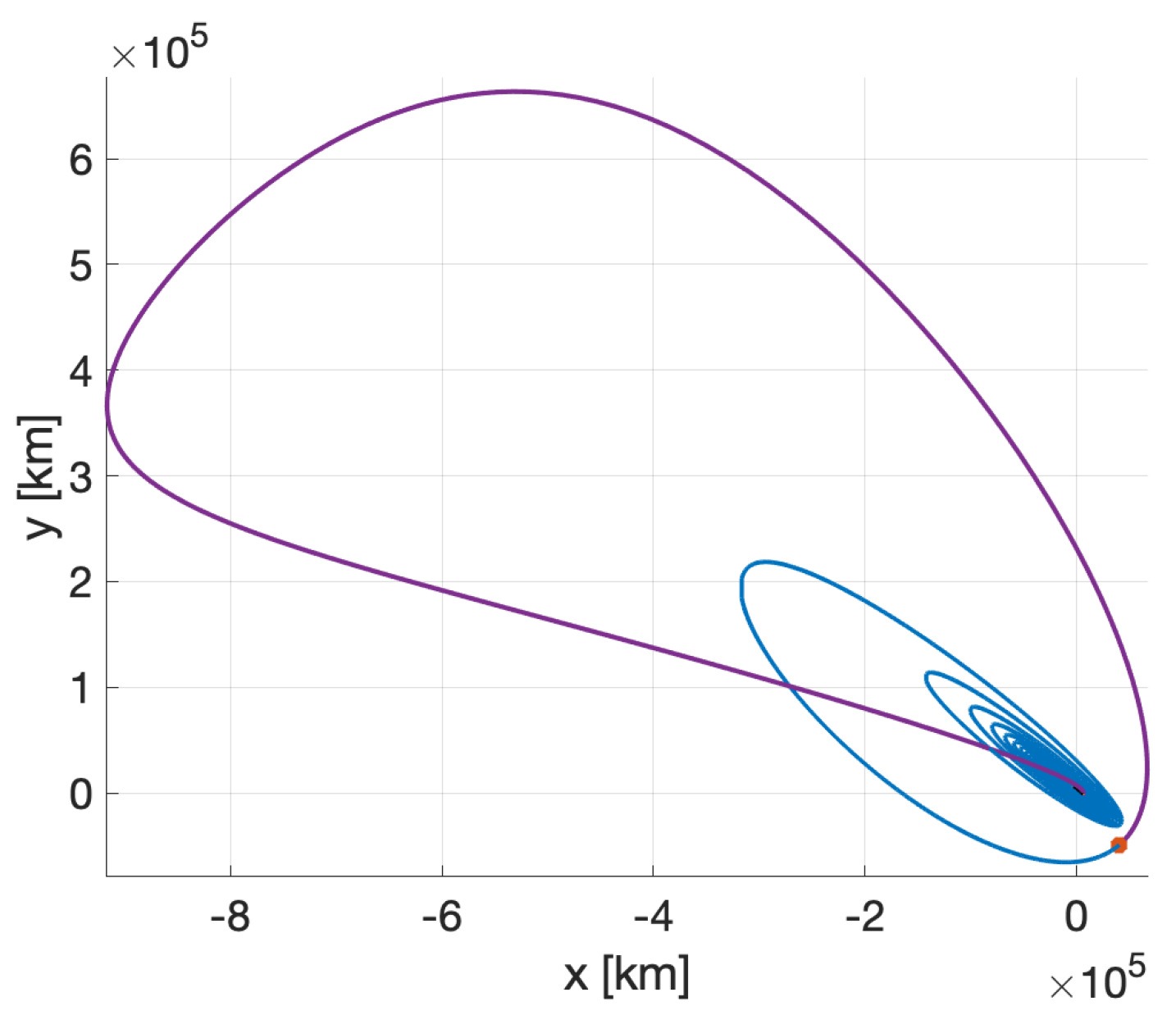
Table 7. Once again, the optimal solution aligns with strategy APO.C, with a mass ratio of 56.10% achieved in 86 days, this time with
. The trajectory undergoes significant deformation due to the gravitational effect of the Sun, as evident in the violet portion of
Figure 9.
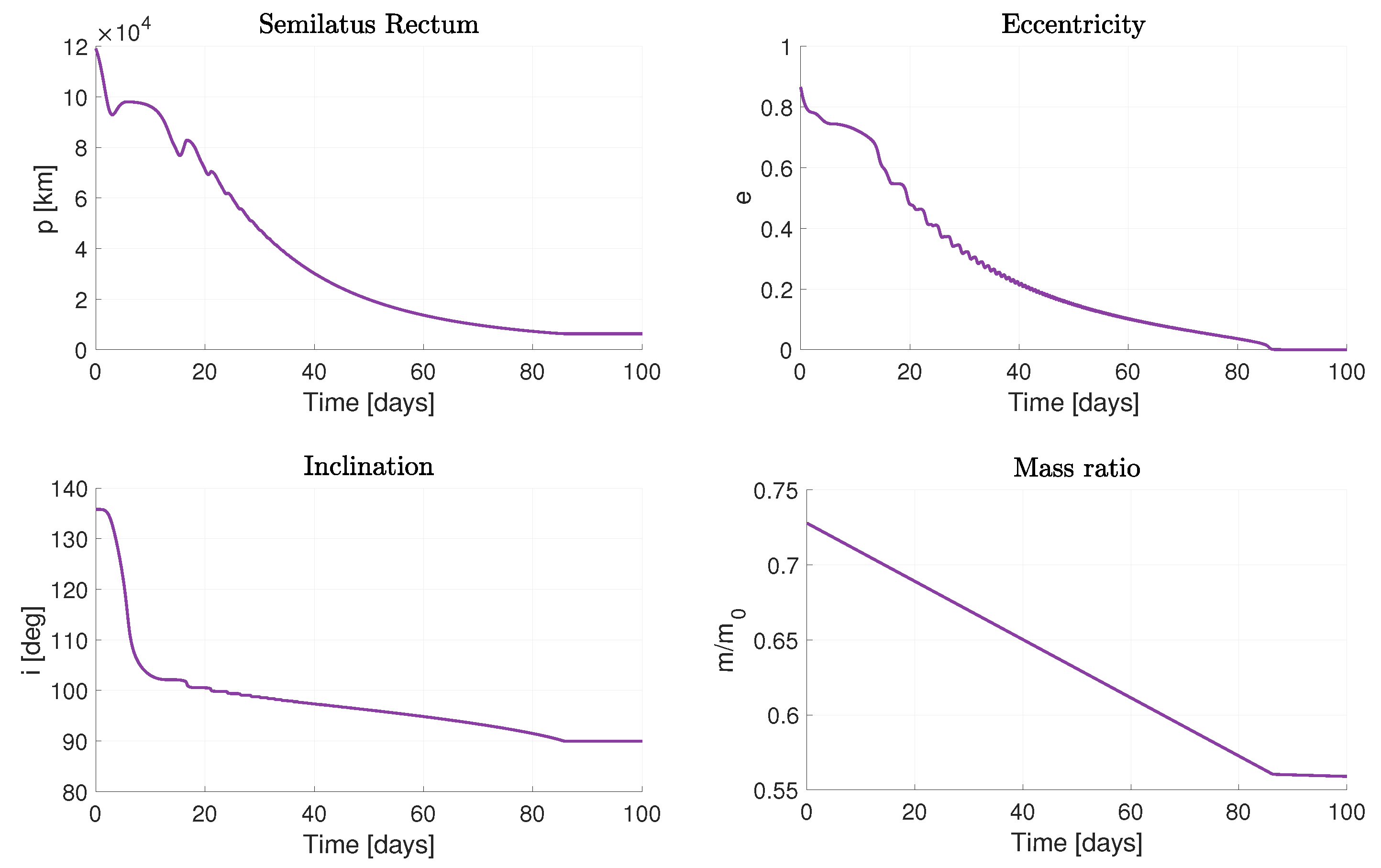
Numerous revolutions around the planet are completed, as often happens in low-thrust applications. The orbit gradually reduces its semimajor axis, eliminating eccentricity at an altitude of 300 km. The corresponding temporal variations of the relevant orbital parameters are presented in
Figure 10. At approximately 86 days, a change in slope is observed in the mass ratio, marking the beginning of the orbit’s station-keeping phase.
5.2. Low-Energy Capture and Low-Thrust Orbit Injection
In this scenario the spacecraft is transferred from the hyperbolic trajectory (interplanetary arc) to a long-term capture orbit by a two-impulse maneuver. The first maneuver is provided during the Venus flyby, at the pericenter, and allows injecting the spacecraft into the equilibrium region surrounding
of the Sun-Venus system. This is achieved providing a
that reduces the energy level from the high value of the interplanetary trajectory
to a lower
compatible with the models described in
Section 2.3. The corresponding
is lower compared to the previously discussed cases in
Section 5.1, as
lies outside Venus’s sphere of influence.
At the entrance into the equilibrium region, the spacecraft dynamical state is characterized by
,
and
, therefore a second maneuver
is performed to establish the long-term capture condition given by Equation (
19) (
).
In this study, energy levels of the order
inside the equilibrium region are considered and the following capture conditions are computed:
km,
km and
km/s. Then a target sequence in GMAT allows determining the hyperbola’s orientation angles at flyby (see
i,
, and
in
Table 5) and
387.9 m/s, applied opposite to the spacecraft’s velocity. From these data, the value
51 m/s is finally determined.
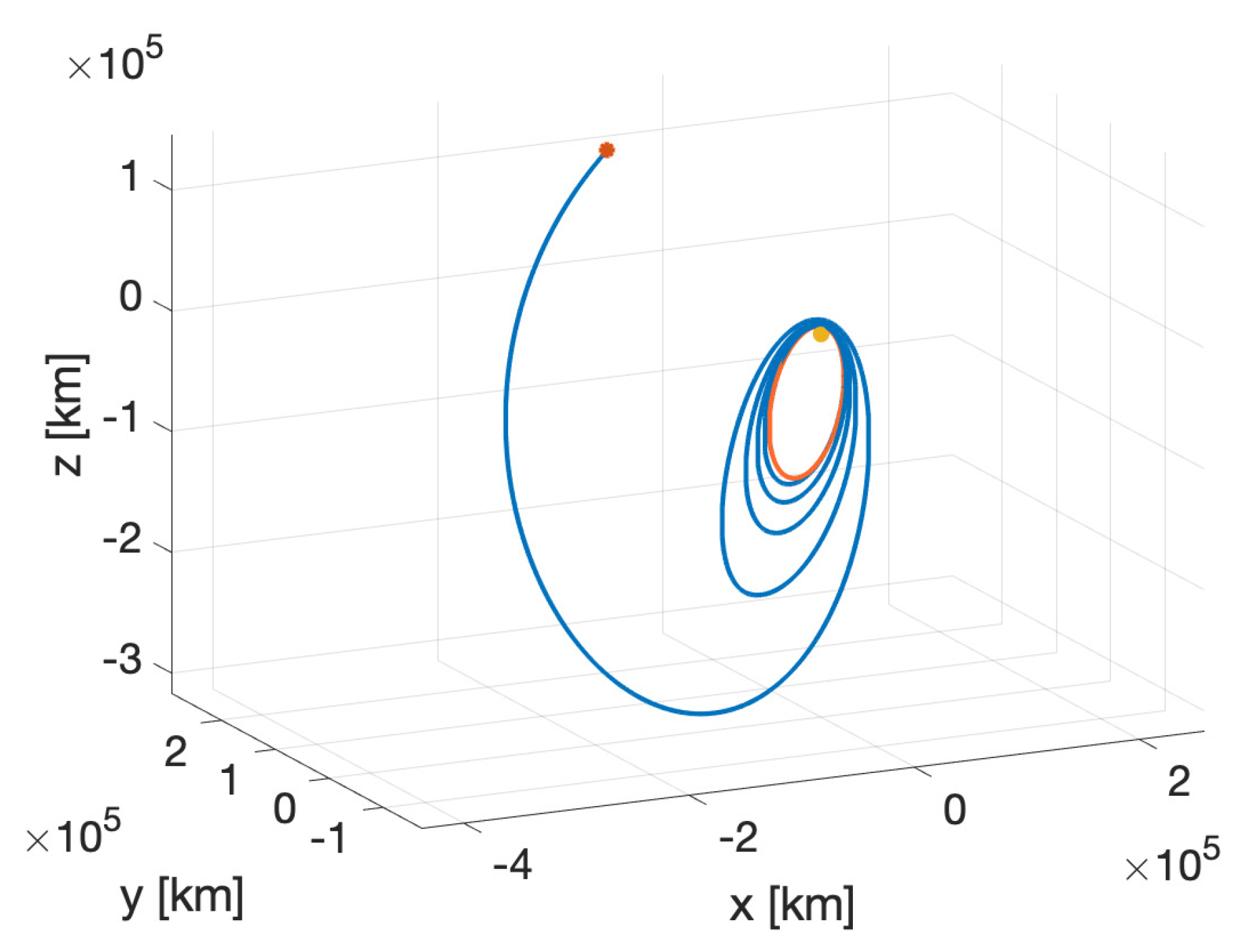
Figure 11 shows the obtained trajectory.
This is a low-energy trajectory that is “trapped” by the planet’s gravitational field for a relatively long period. During this period, low-thrust control is activated, allowing the spacecraft to reach the desired target orbit.
The total delta-v from the start of the mission, entirely associated with chemical propulsion, is calculated as 1041.5 m/s. This corresponds to a mass ratio 70.67%.
Various cases are explored based on the moment of ignition for electric propulsion, identified as “L1.A,” “L1.B,” and “L1.C.” The objective remains to minimize the overall propellant consumption. In the L1.A strategy, low-thrust control is activated one hour after applying within the equilibrium region. In the L1.B strategy, control is activated at the first pericenter (expected to be reached on 2 November 2033) at an altitude of 219,818 km, which already possesses an inclination of approximately 90. Since the trajectory constructed for this scenario with weak capture involves numerous revolutions around the planet, this behavior can be utilized to identify other potential points for low-thrust application over the years. Specifically, reference is made to the subsequent pericenters and apocenters after the first one. Using the same weights as in the L1.B strategy, we examine whether convergence to the target state is achievable at these points.
The attainment of the target elliptical and circular orbits, with orbital elements defined in (
37) and (
38), is now examined. The results are presented in
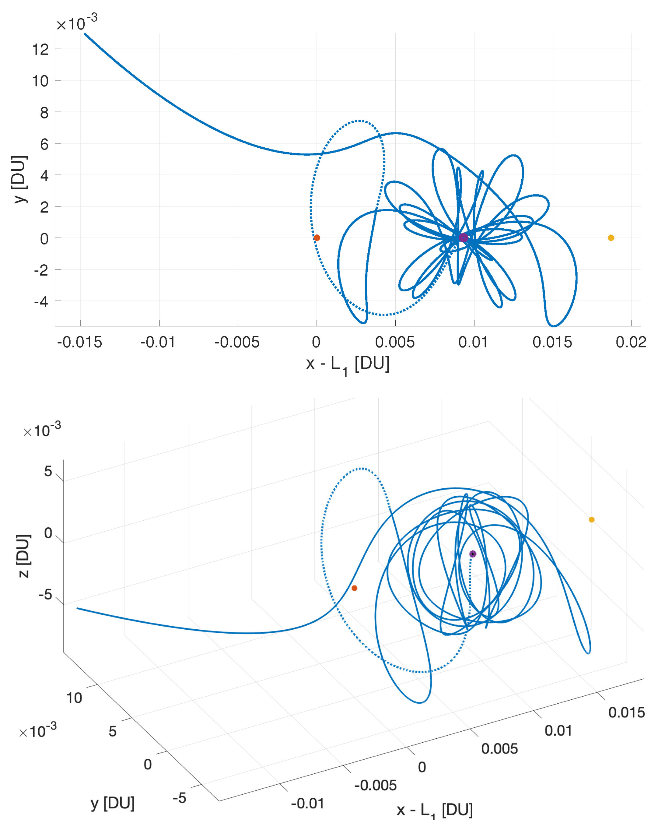
Table 7. The optimal solution for the elliptical target orbit is achieved by activating thrust from the first pericenter at Venus, using strategy L1.B. The trajectory is shown in
Figure 12.
In this case, the inclination at pericenter is already 90
, which provides an advantage. Further exploration using the L1.C strategy for subsequent pericenters and apocenters reveals results depicted in
Figure 13. The optimal solution corresponds to activating control at the first pericenter, resulting in a final mass ratio of 65.82%.
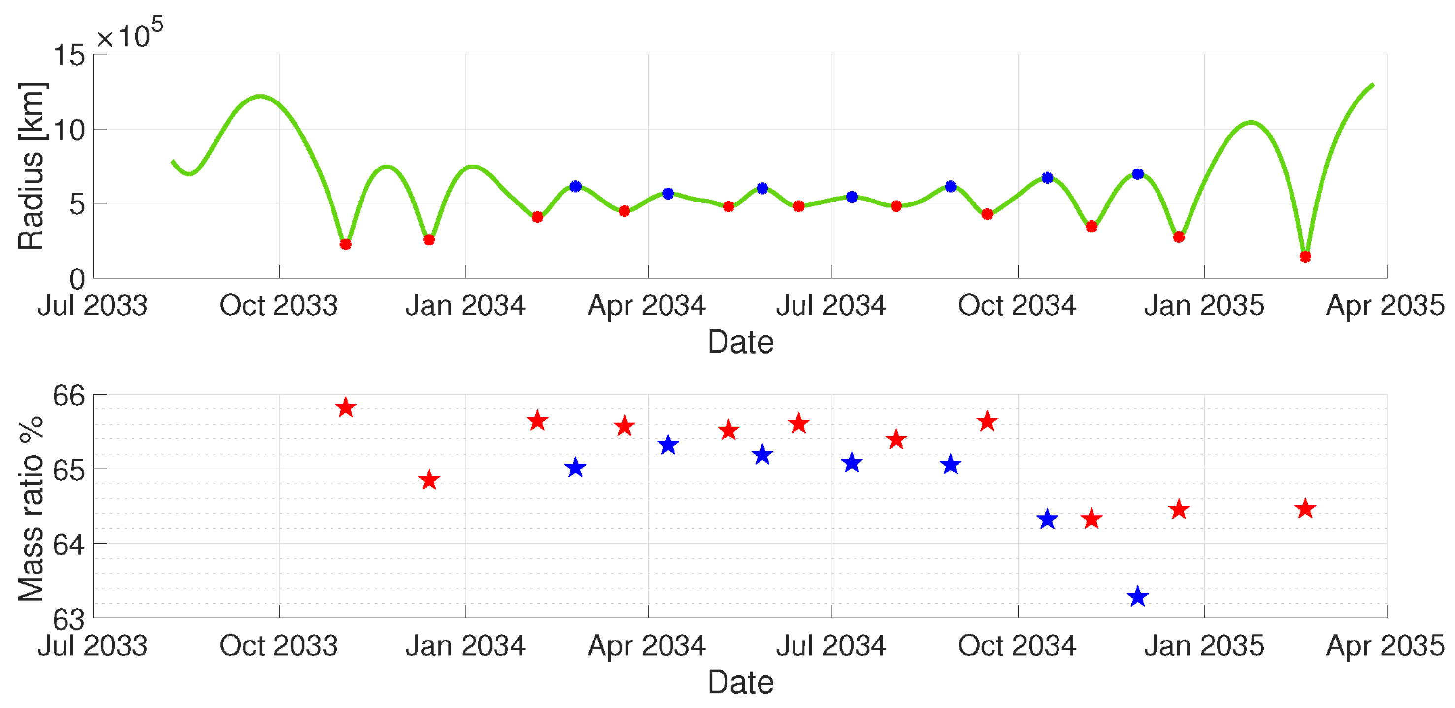
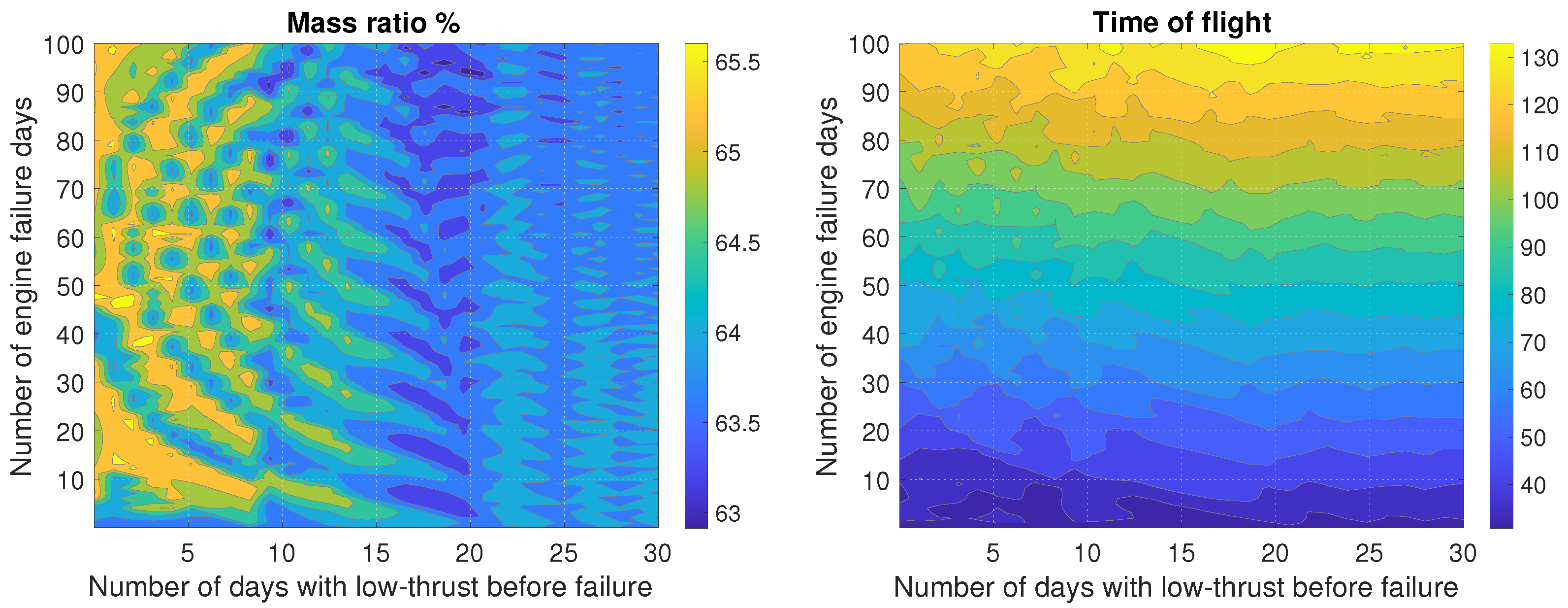
The L1 strategy offers flexible low-thrust control activation for achieving the desired orbit. Real-time adaptability is enabled by a feedback control law, which has been demonstrated to consistently converge to the target state. To validate its effectiveness, simulations are conducted considering temporary propulsion system failure. The L1.B strategy, identified as the most fuel-saving, involves activating low-thrust control at pericenter for
days, followed by a temporary propulsion failure lasting
days. For elliptical orbits, the resulting mass ratio and total flight time vary with
and
, as shown in
Figure 14. A range of
and
is explored, encompassing all scenarios, including delayed control activation (
). Convergence is achieved in all 3000 cases, with higher mass ratio values when the failure occurs within the first 10 days after reaching Venus’s pericenter. The total flight time increases with
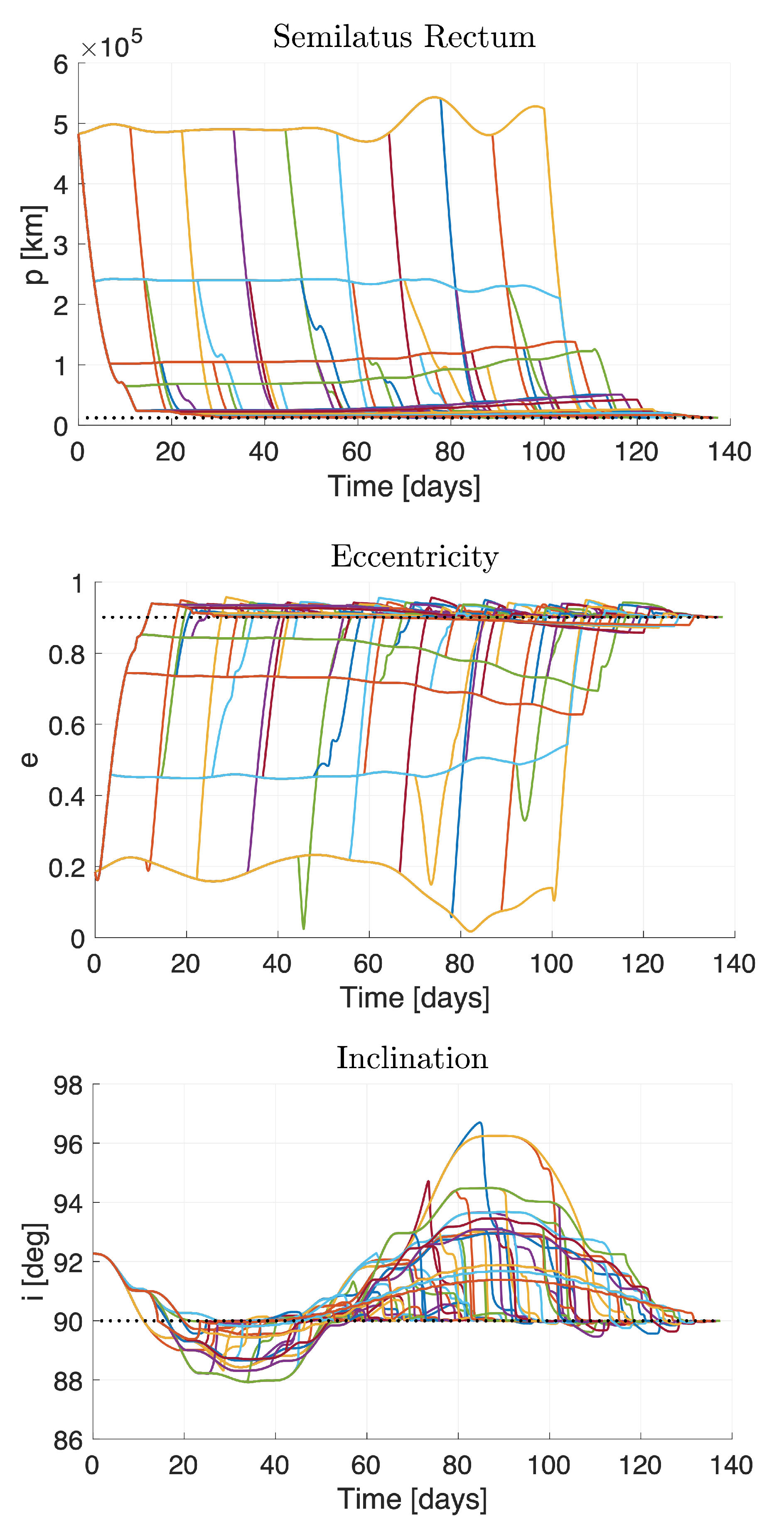
. On average, the mass ratio is 64.26%, with a standard deviation of 0.61%, and the average total flight time is 82.08 days, with a standard deviation of 29.50 days.
Figure 15 displays overlaid profiles for the controlled orbital parameters.
Moving on to achieving a circular orbit, the L1 strategies yield optimal results by initiating low-thrust control once the spacecraft enters orbit around Venus. In this scenario, a slightly superior outcome is attained at the pericenter reached on 19 December 2034, corresponding to a mass ratio of 55.71% compared to 55.70% at the initial pericenter on 2 November 2033. Multiple opportunities exist for implementing low thrust during the capture phase around the planet.
5.3. Discussion of Results
The analysis of different strategies for achieving orbits around Venus has revealed significant findings, demonstrating the effectiveness of both APO and L1 strategies. These strategies combine impulsive maneuvers with chemical propulsion and subsequent low-thrust control using electric propulsion.
For the elliptical target orbit, the APO.C strategy stood out as the most fuel efficient solution, resulting in a final mass ratio of 68.12% achieved within a short time of 10.31 days. In the L1 scenario, the L1.B strategy emerged as the one with the highest final mass ratio of 65.82% and a total flight time of 24.31 days. However, when comparing these results with a traditional strategy that relies solely on optimized impulsive chemical propulsion, with a final mass ratio around 67%, the proposed strategies offer little or no advantage in terms of propellant savings.
For the circular target orbit, the APO strategies achieved mass ratios ranging from approximately 54% to 56%, with the APO.C strategy performing slightly better than the others. On the other hand, the L1 strategies demonstrated favorable outcomes, with the L1.B strategy standing out with a mass ratio of 55.71% and the shortest total flight time of 75 days. When contrasting these outcomes with a specific case with only chemical propulsion, resulting in a mass ratio of approximately 27%, the superiority of the proposed APO and L1 strategies becomes even more evident. These strategies deliver mass ratios that are approximately twice the values with impulsive injection, leading to a substantial enhancement in efficiency and performance. The comparison clearly demonstrates the superiority of the proposed approaches over traditional methods, emphasizing their significant advantage in achieving circular target orbits around Venus.
Furthermore, the analysis considered the impact of temporary propulsion system failure on the L1.B strategy. Simulations demonstrated that convergence to the target state was still attainable in all cases, with the mass ratios deviating only slightly from the nominal case. This highlights the robustness and adaptability of the proposed strategies in real mission scenarios.
6. Concluding Remarks
We developed a novel mission profile to transfer a spacecraft from a highly elliptic Earth orbit to a target orbit around Venus. This study, verified by means of numerical integration, includes a novel approach that (i) combines traditional high-energy interplanetary trajectories with low-energy ones, to transfer the spacecraft into a weak capture orbit at Venus, and (ii) implements a novel nonlinear orbit control using low-thrust propulsion, to inject the spacecraft into the desired final orbit. This mission profile benefits from the use of low-energy arcs and low-thrust propulsion to reduce the propellant mass required for maneuvers, while still allowing for short transfer times, only marginally longer than Earth-Venus transfers designed using a traditional approach.
Two different scenarios were investigated, named as APO and L1. In the APO scenario, an impulsive maneuver performed at the first Venus flyby injects the spacecraft into a highly elliptic orbit and then nonlinear orbit control, implemented by a low-thrust propulsion system, allows transferring it into the desired target orbit. In the L1 scenario, the spacecraft is initially injected into the equilibrium region surrounding Sun-Venus . From here, it is sequentially transferred to a weak capture trajectory and finally, by means of nonlinear orbit control and low-thrust propulsion, into the target orbit.
To evaluate the feasibility of these two options, we performed numerical studies in GMAT and MATLAB, considering departure dates for Venus missions planned between 2028 and 2033. If compared to a traditional (impulsive) strategy, the proposed mission profiles result in significant savings in the propellant mass. Specifically, the propellant usage reduces from the 73% to the 44% for the APO strategy and to the 45% for the L1 strategy, considering a circular target orbit around Venus. Even-though the L1 scenario requires an additional mid-course interplanetary maneuver (DSM) and is less favorable with respect to the APO scenario, it enhances the mission flexibility and reliability, since the low-thrust propulsion system can be actuated at any apocenter or pericenter of the low-energy capture orbit ensuring successful injection into the target orbit.
Furthermore, our research proves that delaying the injection into the low-energy capture trajectory from the beginning of the interplanetary arc to its end can lead to savings in the total transfer time. While low-energy transfers from Earth to Venus can take up to 300% more time than traditional ones, the L1 scenario demonstrates a better outcome, with only a 56% increase in total transfer time.
In conclusion, the proposed novel mission profiles, leveraging low-energy trajectories and low-thrust propulsion, offer significant propellant savings and improved mission efficiency, making them promising candidates for future interplanetary missions from Earth to Venus.


