Article

Aerodynamic Robust Design Research Using Adjoint-Based Optimization under Operating Uncertainties

1
School of Aeronautics, Northwestern Polytechnical University, Xi’an 710072, China
2
State Key Laboratory for Strength and Vibration of Mechanical Structures, School of Aerospace Engineering, Xi’an Jiaotong University, Xi’an 710049, China
3
AVIC The First Aircraft Institute, Xi’an 710089, China
*
Author to whom correspondence should be addressed.
Aerospace 2023, 10(10), 831; https://doi.org/10.3390/aerospace10100831
Submission received: 5 August 2023 / Revised: 20 September 2023 / Accepted: 21 September 2023 / Published: 24 September 2023
(This article belongs to the Special Issue Adjoint Method for Aerodynamic Design and Other Applications in CFD)

Abstract

:
Robust optimization design (ROD) is playing an increasingly significant role in aerodynamic shape optimization and aircraft design. However, an efficient ROD framework that couples uncertainty quantification (UQ) and a powerful optimization algorithm for three-dimensional configurations is lacking. In addition, it is very important to reveal the maintenance mechanism of aerodynamic robustness from the design viewpoint. This paper first combines gradient-based optimization using the discrete adjoint-based approach with the polynomial chaos expansion (PCE) method to establish the ROD framework. A flying-wing configuration is optimized using deterministic optimization and ROD methods, respectively. The uncertainty parameters are Mach and the angle of attack. The ROD framework with the mean as an objective achieves better robustness with a lower mean (6.7% reduction) and standard derivation (Std, 18.92% reduction) compared to deterministic results. Moreover, we only sacrifice a minor amount of the aerodynamic performance (an increment of 0.64 counts in the drag coefficient). In comparison, the ROD with Std as an objective obtains a very different result, achieving the lowest Std and largest mean The far-field drag decomposition method is applied to compute the statistical moment variation of drag components and reveal how the ROD framework adjusts the drag component to realize better aerodynamic robustness. The ROD with the mean as the objective decreases the statistical moment of each drag component to improve aerodynamic robustness. In contrast, the ROD with Std as an objective reduces Std significantly by maintaining the inverse correlation relationship between the induced drag and viscous drag with an uncertainty parameter, respectively. The established ROD framework can be applied to future engineering applications that consider uncertainties. The unveiled mechanism for maintaining aerodynamic robustness will help designers understand ROD results more deeply, enabling them to reasonably construct ROD optimization problems.

1. Introduction

The traditional aerodynamic design operates as a deterministic process, which may cause the aerodynamic performance to be extremely sensitive to uncertainty parameters (operating conditions and manufacturing), or can bring about certain security risks [1]. Zang [2] has summarized the needs and opportunities for multidisciplinary design methods under uncertainty influences for aerospace vehicles, including aerodynamic design. Optimization that considers uncertainties, such as those in operating conditions, is known as robust optimization design (ROD). Huyse and Lewis [3] and Walters and Huyse [4] applied ROD to two-dimensional airfoils; the results show obvious differences between deterministic optimization and ROD, emphasizing the significance of considering uncertainty parameters.
Computational fluid dynamics (CFD) and optimization algorithms have matured in the realm of aerodynamic optimization design [5,6,7,8,9]. Moreover, drag production analysis tools are being utilized for research into aerodynamic mechanisms, such as using the far-filed decomposition method [10]. The primary objective in developing ROD is to combine the existing advanced CFD and optimization approaches with uncertainty quantification methods to achieve efficient and robust aerodynamic optimization design.
Depending on whether the optimization algorithm relies on gradients, both gradient-based and gradient-free ROD approaches are being researched and developed. Dodson and Parks [11] used a non-intrusive PCE method in conjunction with CFD and differential evolution (DE) for robust optimization. The objective is to maximize the lift-to-drag ration for a two-dimensional airfoil while minimizing its sensitivity to uncertainty in the leading-edge thickness. Compared to the deterministic optimization result, the robust optimization is significantly less sensitive to input variations. Wang et al. [12] proposed an efficient and robust aerodynamic optimization method based on the PCE model and the multi-objective genetic algorithm (MOGA) for compressor optimization.
Sabater et al. [13] developed a ROD framework based on CFD, linear stability theory, and surrogate models, specifically for laminar flow wings. The bi-level surrogate model is applied; it combines a surrogate-based optimization framework as an outer layer, with a surrogate-based uncertainty quantification framework in the inner layer. The critical N factors are taken as uncertainty parameters. The ROD results are more balanced than the deterministic optimization results since the transition smoothly moves upstream as the critical N factors (Tollmien–Schlichting and cross-flow instabilities) are reduced.
We will now focus on gradient-based ROD research. Sriram and Jameson [14] combined Euler equations and the corresponding adjoint with the non-intrusive PCE method for robust optimal control. The ROD implementation and stochastic investigation on an airfoil highlight the significance of considering uncertain inputs. A novel reduced quadrature technique [15] is used in the gradient-based ROD of aerodynamic shapes. The CFD code used for this study couples the full potential equations in the inviscid flow region with the integral equations representing the viscous flow region. A robust optimization problem that focuses on the conceptual design of a transonic airfoil shows that the solutions considering uncertainty parameters can outperform the deterministic solution.
Moreover, low-fidelity models are insufficient at capturing dominant trade-offs [16], leading to the development of ROD based on high-fidelity CFD (RANS-based solver). Mura et al. [17] discussed the efficiency and flexibility of least squares surrogates and gradient-enhanced PCE for uncertainty quantification and robust optimization based on the gradient-based algorithm. The proposed method’s advantages over collocation approaches were verified using the NACA0012 airfoil under transonic conditions. Based on adjoint gradient-based optimization, Jofre and Doostan [18] proposed a stochastic gradient approach to perform the rapid aerodynamic shape optimization under uncertainty. The NACA0012 airfoil optimization under operating conditions and turbulence model uncertainty was implemented. The results show that the stochastic gradient approach significantly improves the aerodynamic design’s performance across a broad spectrum of operating conditions and turbulence models.
For the modern refined aircraft design, it faces the “curse of dimensionality” problem. Currently, gradient-based optimization algorithms are the only viable way to handle optimization problems with larger numbers of variables [6]. The discrete adjoint-based method ensures that a large number of derivatives can be computed in an accurate and efficient way, taking full advantage of gradient-based optimization algorithms. The adjoint-based gradient optimization with high-fidelity CFD simulation has been widely used in aerodynamic shape optimization in engineering applications [19,20,21,22,23,24,25]. Thus, the adjoint-based gradient optimization approach would be a good basis for developing the ROD framework.
As discussed previously, the non-intrusive PCE method is frequently applied and is a prime candidate in the aerodynamic ROD and sensitivity analysis due to its attainability and high accuracy at reasonable costs [26,27,28]. Moreover, the PCE method uses the sum of orthogonal polynomials with independent random variables to simulate random processes without random sampling, and can directly obtain relevant statistical moment information through analytical expressions. The mathematical principle of PCE makes it compatible with the existing gradient optimization method system based on the adjoint method. Thus, the PCE method coupled with the adjoint gradient-based optimization algorithm would be a powerful ROD tool. Meanwhile, the information from the derivatives helps to improve PCE efficiency at the given sampling points [29]. Reviewing the development of ROD based on PCE reveals that most implementations have been verified and applied to two-dimensional airfoils, while a three-dimensional aircraft ROD framework and application are required.
For practical three-dimensional aerodynamic problems, the optimizations can only provide optimization results. The drag production analysis (such as far-field drag decomposition) together with the sensitivity analysis can explain the formation mechanism of uncertainty production, and assist designers in reasonably constructing ROD optimization problems to improve optimization results and efficiency. However, research on far-field drag decomposition (to explain and analyze ROD results) is still missing.
Based on the developments made by researchers and the analysis discussed previously, this paper mainly contributes in several ways. We construct an efficient and reliable ROD framework-based PCE method and adjoint-based gradient algorithm, using a high-fidelity CFD simulation. For the uncertainty quantification, the derivatives and sparsity-of-effects are researched to improve the PCE efficiency. The far-field drag decomposition and sensitivity analysis in the ROD framework are then applied and coupled to explain the ROD results. Significantly, a three-dimensional flying-wing configuration concerned in the engineering application is optimized using the ROD framework and the maintenance mechanism of aerodynamic robustness is researched.
This paper is constructed as follows. The non-intrusive PCE method and global sensitivity analysis based on PCE are first introduced in Section 2. We then establish the adjoint-based ROD framework based on MACH-Aero and the PCE method (Section 3). The statistical moment derivatives are computed to operate gradient-based optimization. In Section 4, the far-field drag decomposition is introduced and verified. We further apply our established ROD work and stochastic investigation to a flying-wing configuration in Section 5. We finally summarize our work in Section 6.

2. Uncertainty Quantification and Global Sensitivity Analysis Approach

2.1. Polynomial Chaos Expansions

We rely on the PCE to approximate the quantity of interest (QoI). The input random variables, Ξ = { Ξ k | k = 1 , 2 , . . . , d } , are independent and described by the probability density function (PDF). The stochastic model with Ξ can be defined as Y = f ( Ξ ) . For the stochastic analysis of Y , the model f ( Ξ ) can be approximated by
Y = j = 0 c j Ψ j ( Ξ ) .
The coefficients c j are the expansion coefficients, which are dependent on the deterministic input variables X = { X i | i = 1 , 2 , . . . , n } .
In Equation (1), Ψ j ( Ξ ) are the multivariate orthogonal polynomials and are constructed using the tensor product of the univariate orthogonal polynomials with respect to the corresponding marginal PDF, as follows:
Ψ α ( Ξ ) = k = 1 d φ k α k Ξ k ,
where φ k α k is the univariate orthogonal polynomial ( { φ k 0 ( Ξ k ) , φ k 1 ( Ξ k ) , , φ k p ( Ξ k ) } ) with degree α k for the random variable Ξ k . In practice, the PCE Equation (1) is truncated to the set of P + 1 basis functions associated with the subspace of polynomials of a total-order no greater than p, which is k = 1 d α k p . To improve the computation efficiency, a hyperbolic index set Λ p , q d (q-quasi-norms) can be used, then Equation (1) can be written as
Y ( Ξ ) = α Λ p , q d c α Ψ α ( Ξ ) .
The total-degree basis of degree p is given by
Λ p , q d = { Ψ α : | | α | | q p } ,   α = { α 1 , , α d } .
When q (sparse coefficient) is equal to 1, it corresponds to the usual truncation scheme, and the total number of terms P + 1 in the polynomial is computed as
P + 1 = ( p + d ) ! p ! d ! .
The use of norms penalizes the high-rank indices all the more. This favors the main effects and low-order interactions, which are more likely to be significant than the high-order interactions in the governing equations of the model, according to the sparsity-of-effects principle [30].
The key of PCE computes the coefficients c = c 0 , , c P . We use the collocation technique and linear regression-based method to obtain the coefficients. The regression-based method aims to build a surrogate model of the PCE. The PCE approximation for a response Y using regression can be given as
Y = Ψ c + ε ,
where ε is the truncation error. For a given design of experiment (DOE) with size N s and corresponding function evaluations Y = { y 1 , . . . , y N s } T , dropping the truncation error gives us a linear system:
Ψ c = Y ,
and can be further expressed as
Ψ 0 Ξ 1 Ψ 1 Ξ 1 Ψ P Ξ 1 Ψ 0 Ξ 2 Ψ 1 Ξ 2 Ψ P Ξ 2 Ψ 0 Ξ N s Ψ 1 Ξ N s Ψ P Ξ N s c 1 c 2 c P = Y 1 Y 2 Y N s .
Ψ represents a measurement matrix of size N s × ( P + 1 ) and has components Ψ i j = Ψ j ( Ξ i ) . The least-squares approach involves minimizing the sum of the squares of the squares of residuals in Equation (6), i.e., min | | Ψ c Y | | 2 . The coefficients are obtained by c = Ψ T Ψ 1 Ψ T Y . In general, it is suggested that the number of samples be greater than the number of PCE terms, i.e., N s > P + 1 , to improve the accuracy. The oversampling ratio n p is given, and the total sampling number is N s = n p ( P + 1 ) .

2.2. Gradient-enhanced Polynomial Chaos Expansions

It has been found that PCE coefficients can be obtained with a comparable level of accuracy but significantly fewer sampling points if the gradient information (gradient-enhanced PCE, GEPCE) is provided [17,31]. Since the linear system of the PCE coefficients (Equation (8)) is not underdetermined, the number of sampling points can be reduced by simply writing a number of additional equations to achieve full rank. For the k-th point, we have
Y ( Ξ k ) = j = 1 N s c j Ψ j ( Ξ k ) .
With differentiation, Equation (9) is expressed as
Y ( Ξ k ) Ξ j = j = 1 N s c j Ψ j ( Ξ k ) Ξ j .
Finally, we extend Equation (8) as
Ψ 0 Ξ 1 Ψ 1 Ξ 1 Ψ P Ξ 1 Ψ 0 Ξ 1 Ξ 1 Ψ 1 Ξ 1 Ξ 1 Ψ P Ξ 1 Ξ 1 Ψ 0 Ξ 1 Ξ n Ψ 1 Ξ 1 Ξ n Ψ P Ξ 1 Ξ n Ψ 0 Ξ 2 Ψ 1 Ξ 2 Ψ P Ξ 2 Ψ 0 Ξ 2 Ξ 1 Ψ 1 Ξ 2 Ξ 1 Ψ P Ξ 2 Ξ 1 Ψ 0 Ξ 2 Ξ n Ψ 1 Ξ 2 Ξ n Ψ P Ξ 2 Ξ n Ψ 0 Ξ N s Ψ 1 Ξ N s Ψ P Ξ N s Ψ 0 Ξ N s Ξ 1 Ψ 1 Ξ N s Ξ 1 Ψ P Ξ N s Ξ 1 Ψ 0 Ξ N s Ξ n Ψ 1 Ξ N s Ξ n Ψ P Ξ N s Ξ n c 0 c 1 c P = Y Ξ 1 Y Ξ 1 Ξ 1 Y Ξ 1 Ξ n Y Ξ 2 Y Ξ 2 Ξ 1 Y Ξ 2 Ξ n Y Ξ N s Y Ξ N s Ξ 1 Y Ξ N s Ξ n .
For each point, n more equations become available. The ratio between the minimal required number of points without and with gradient information is ( n + 1 ) , regardless of the expansion order. For the left side of Equation (11), the gradient of Ψ j / Ξ i can be derived analytically. The gradients on the right side of Equation (11) ( Y i / Ξ i ) are computed by using the gradients of the deterministic sampling points.
When we obtain the coefficients c by using PCE or GEPCE, the mean and variance can be computed according to
f ( Ξ ) μ Y = E ( Y ) = f ( Ξ ) w ( Ξ ) d Ξ = j = 0 P c j Ψ j w ( Ξ ) d Ξ = j = 0 P c j Ψ j w ( Ξ ) d Ξ .
where w ( Ξ ) is the joint PDF. For every PDF w ( Ξ ) , there exists < Ψ j ( Ξ ) , Ψ i ( Ξ ) > : = Ψ j ( Ξ ) Ψ i ( Ξ ) d Ξ = 0 ( i j ) . Being Ψ 0 = 1 , Ψ j w ( Ξ ) d Ξ is zero for every j > 0 . Thus, we have
μ Y = c 0 .
For the variance, we have
σ 2 ( Y ) = E ( Y E ( Y ) ) = ( j = 0 P c j Ψ j c 0 ) 2 w ( Ξ ) d Ξ = ( j = 1 P c j Ψ j ) 2 w ( Ξ ) d Ξ = j = 1 P c j c j Ψ j 2 w ( Ξ ) d Ξ = j = 1 P c j 2 | | Ψ j | | 2 = j = 1 P c j 2 ,
where < Ψ j , Ψ j > is 1 as the polynomial basis functions are normalized.
In addition, the normal root mean square deviation (NRMSD) is used for the precision measurement, i.e.,
NRMSD = 1 n i = 1 n ( Y ˜ i Y i ) 2 max ( Y ) min ( Y ) .

2.3. Global Sensitivity Analysis

To estimate the relative contribution of each uncertainty input variable, we choose the global sensitivity analysis method, denoted as Sobol indices. For the model of Y = f ( Ξ ) , the input parameters are defined on the d-dimensional independent vector, i.e., Ξ = { Ξ 1 , . . . , Ξ d } . Sobol’s decomposition of f ( Ξ ) into the summands of increasing dimension reads [32]
f ( Ξ ) = f 0 + k d f k ( Ξ k ) + k < i d f ki ( Ξ k , Ξ i ) + + f 1 , , d ( Ξ 1 , , Ξ d ) .
This decomposition is unique if conditions 0 1 f k 1 k s d Ξ k j = 0 for 1 j s are satisfied. Here 1 k 1 < < k s d . By integrating the square of Equation (16) and by using the condition of 0 1 f k 1 k s d Ξ k j = 0 for 1 j s , the total variance can be decomposed as follows:
V = k = 1 d V k + k i V ki + + V 1 , 2 , , d ,
where the partial variances are described as
V k 1 , , k s = f k 1 , , k s 2 ( Ξ k 1 , , Ξ k s ) d Ξ k 1 , , d Ξ k s ,
where there exists 1 k 1 < k s d , s = 1 , , d .
The Sobol indices are defined as
S k 1 , , k s = V k 1 , , k s / V .
By definition, according to Equation (18), there exists
k = 1 d S k + k i S ki + + S 1 , 2 , , d = 1 .
As a consequence, each index S k 1 , , k s is a sensitivity measure that describes the proportion of the total variance due to the uncertainties in the set of input variables { k 1 , , k s } . The first-order indices S k estimate the influence of each parameter taken alone, and are described as
S k = Var Ξ k ( E ( Y | Ξ k ) ) V = α { k 1 , , k s } c α 2 E ( Ψ α 2 ) j = 1 P c j 2 E ( Ψ j 2 ( Ξ ) ) ,
whereas, the higher-order indices account for the possible mixed influences of various uncertainties. The variance-based total sensitivity index S T k is defined as the sum of all partial sensitivity indices V k 1 , , k s involving parameter k,
S T k = E ( Var Ξ k ( Y | Ξ k ) ) V = 1 Var Ξ k ( E Ξ k ( Y | Ξ k ) ) V = ( k 1 , , k s ) J ( i 1 , , i t ) V k 1 , , k s j = 1 P c j 2 E ( Ψ j 2 ( Ξ ) ) .
where Ξ k indicates the exclusion of input parameter Ξ k , and J i 1 , , i t = { ( k 1 , , k s ) , ( i 1 , , i t ) ( k 1 , , k s ) } .
Once the PCE model is established and correspondent coefficients are obtained, the Sobol sensitivity indices of the system of output responses can be obtained [33]. Therefore, the PCE-based global sensitivity analysis is widely used in engineering applications [34,35,36].

2.4. Ishigami Test Case

Take the Ishigami function [37] into consideration:
Y = f ( X ) = sin X 1 + a sin 2 X 2 + b X 3 4 sin X 1 ,
where the stochastic input variables are independent and are subject to a uniform distribution, i.e., X 1 , X 2 , X 3 U ( π , π ) . The values of a and b are 7 and 0.1 , respectively. The theoretical mean and variance are
E ( Y ) = a 2 = 3.5 , σ 2 ( Y ) = 1 2 + a 2 8 + b 2 π 8 18 + b π 4 5 = 13.844587940719254 .
Sobol’s decomposition variances are
V 1 = 1 2 1 + b π 4 5 2 , V 2 = a 2 8 , V 1 , 3 = b 2 π 8 8 255
and V 3 = V 1 , 2 = V 2 , 3 = V 1 , 2 , 3 = 0 . This leads to the following first-order Sobol indices:
S 1 = V 1 σ 2 ( Y ) ,   S 2 = V 2 σ 2 ( Y ) ,   S 3 = 0 ,
and the following total-order indices:
S T 1 = V 1 + V 1 , 3 σ 2 ( Y ) ,   S T 2 = S 2 ,   S T 3 = V 1 , 3 σ 2 ( Y ) .
We use the Ishigami function to verify the precision of hyperbolic PCE and the GEPCE method, or their combination. The sparse coefficient q is defined as 1.0, 0.5, and 0.7. The order p ranges from 1 to 20, and the sampling number is from 10 to 300. The relative error is defined as ε I = | I PCE I theroy | / I theroy . The corresponding precision comparison with the difference parameter settings is shown in Table 1. The oversampling ratios are selected as n p = 1 and n p = 2 , respectively. We show the order, sampling number, and oversampling ratio when NRMSD is lower than 0.3%, which is an acceptable error in engineering applications. From the comparison results, the sparse coefficient q could help lower the sampling number (PCE, PCE-Sparse0.5, and PCE-Sparse0.7). The oversampling ratio helps to reduce the sampling number slightly, but it might also cause an overfitting problem. The gradient information greatly improves the efficiency of the PCE model. When we combine sparse techniques, appropriate sparse coefficients would help to further reduce the sampling number (GEPCE and GEPCE-Sparse0.7). If we use the oversampling ratio on GEPCE, it does not help to improve the efficiency, and the required sampling number is increased a lot. Comparing all the results, the GEPCE with the appropriate sparse coefficient proves to be an efficient and accurate combination for approximating the QoI.
We also implement the global sensitivity analysis with GEPCE and the sparse technique (Table 2). When we apply the GEPCE with p = 8 (136 sampling number), and a combination of GEPCE and the sparse technique with q = 0.7 , p = 8 (100 sampling number), the relative error compared with theoretical solutions could be lower than 0.5%. With the increase of order p, the relative error is reduced a lot, lower than 10 4 . For the GEPCE with p = 13 , the sampling number is 274; while for the GEPCE with q = 0.7 , p = 15 , the sampling number is 223. From the first-order Sobol indices, the third uncertainty parameter X 3 has no influence on the QoI. The first two uncertainty parameters ( X 1 and X 2 ) are the main contributing factors.

3. Adjoint-Based Robust Optimization Design Framework

We use the high-fidelity aircraft design optimization tool as the basis, i.e., the MDO of aircraft configurations with high fidelity (MACH-Aero) https://github.com/mdolab/MACH-Aero. In this paper, we incorporate uncertainty quantification, compute its gradients, and discuss the sampling method employed for the PCE model. In this section, we mainly introduce the RANS solver and detail the computation of derivatives, statistical moment computations, and their respective derivative computations, along with the ROD framework.

3.1. RANS-Based CFD Solver and Its Adjoint Equation

We use the open-source solver (ADflow https://github.com/mdolab/ADflow). ADflow is a finite-volume structured multi-block and overset mesh solver [6]. We focus on three-dimensional, steady-state turbulent flow equations (RANS equations). ADflow supports several turbulence models, including the one-equation SA model [38] and the two-equation Menter shear stress transport (SST) model [39]. Herein, we use the SA model. In ADflow, the inviscid fluxes are discretized by using different numerical schemes, and we use the Jameson–Schmidt–Turkel (JST) artificial dissipation scheme. The viscous fluxes use standard central differencing. The solver addresses steady flow by alternating between different numerical algorithms, including a Runge–Kutta (RK) algorithm, a diagonal dominant alternating direction implicit (D3ADI) scheme, an approximate Newton–Krylov (ANK) algorithm [40], and a full Newton–Krylov (NK) algorithm. We can combine RK or D3ADI with ANK or NK, or both. The combination of ANK and NK is also a good choice. Finally, we converge the residuals R ( x , q ) of the governing equations to an acceptable tolerance, and x , q are the design variables and state variables (three-dimensional velocities ( u , w , v ) , pressure p, total energy E, and ν ˜ of the SA model).
The discrete adjoint method assumes that a discretized form of the RANS equations meets
R ( x , q ) = 0 .
The functions of interest are functions of both design variables ( x ) and the state variables ( q ), i.e.,
I = I ( x , q ) .
The derivative of d I d x can be described by the chain rule:
d I d x = I x + I q d q d x .
The derivatives of d q / d x are expensive since q is implicitly determined by the residual equations R ( q , x ) = 0 . Whereas, since the partial derivatives I / x and I / q only involve explicit computations, they cost much less.
To compute d q / d x , we differentiate the residual equations, and we obtain
R x = R q d q d x .
As a result, d q / d x = [ R / q ] 1 [ R / x ] . Then, we have
d I d x = I x I q R q 1 ϕ T R x .
A linear system can be written as
R q T ϕ = I q ,
avoiding the very expensive computations (a huge number of computations) of residual equations; Equation (28). In the adjoint equation (Equation (33)), ϕ is denoted as the adjoint vector. The total derivatives are then computed as
d I d x = I x ϕ T d q d x .
Since the design variables do not explicitly appear in Equation (33), we only need to solve the adjoint equation once. In other words, the computational cost is almost independent of the number of design variables. From Equation (34), the computational cost is proportional to the number of functions of interest. For the aircraft design, the adjoint method has a huge advantage because the functions of interest are no more than 10, while the design variables can be hundreds to thousands. In ADflow, the chain rule, automatic differentiation, and Jacobian-free technique are used to obtain the Jacobian matrix vector in the adjoint equation and the partial derivatives in the total derivatives. The generalized minimal residual (GMRES) algorithm is applied to solve the adjoint equation.

3.2. Derivatives Computation of Statistic Moment
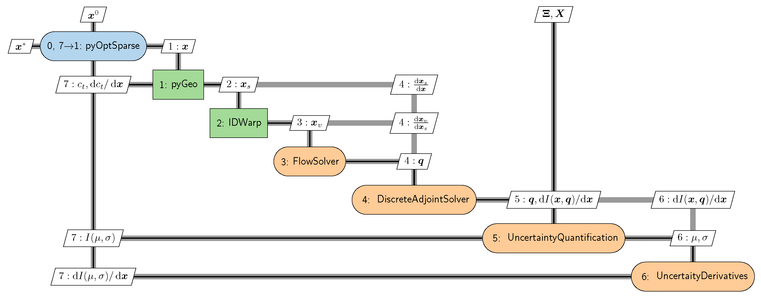
For the deterministic optimization, the objectives are functions of interest, i.e.,
Min I ( x ) .
Whereas, the objective function of the ROD can be a linear combination of the mean and Std, or the mean, or the Std. To implement the gradient-based ROD, the derivatives of statistical moments are required, i.e., d μ Y / d x and d σ Y / d x . From Equations (13) and (14), the derivatives of the mean and variance can be expressed as
d μ Y d x = d d x < Y > = d Y d x ,
and
d σ Y 2 d x = j = 1 P c j 2 d x = 2 j = 1 P c j d c j d x .
Then, we would obtain the derivatives of the Std with respect to the design variables
d σ Y d x = = 1 2 σ d σ Y 2 d x = 1 σ j = 1 P c j d c j d x .
The key is to compute d c j / d x . We differentiate Equation (1) from the set of P + 1 basis functions, i.e.,
Y x i = j = 0 P d c j ( x ) d x i Ψ j ( Ξ ) ,
where the left side values, Y / x i , are computed by deterministic samplings using the adjoint method. The x i is the i-th design variable. The Ψ j ( Ξ ) is determined by the established PCE model. Subsequently, we can construct a new PCE model; the coefficients are d c j / d x , denoted as b j i . For the i-th design variable, the linear system is constructed as
Ψ 0 Ξ 1 Ψ 1 Ξ 1 Ψ P Ξ 1 Ψ 0 Ξ 2 Ψ 1 Ξ 2 Ψ P Ξ 2 Ψ 0 Ξ N s Ψ 1 Ξ N s Ψ P Ξ N s b 0 i b 1 i b P i = Y Ξ 1 x i Y Ξ 2 x i Y Ξ N s x i .
We have N linear systems (N design variables). When the d c j / d x is obtained, we obtain the objective functions of ROD with respect to deterministic design variables. The derivatives are the input to the gradient-based optimization framework.

3.3. ROD Framework

The whole ROD framework is constructed in Figure 1. In Figure 1, x denotes the deterministic design variables. x s and x v are the surface and volume coordinates. The FFD (free-form deformation) method connects the control frame (control points) with the surface coordinates. When the control points change, the concerned geometry deforms continuously, and we obtain the updated surface coordinates. We use the open-source FFD code (pyGeo https://github.com/mdolab/pygeo); this code also provides the derivatives of d x s / d x . After we obtain the updated surface coordinates, a moving mesh wrapping is required to obtain the new volume mesh. The IDwarp https://github.com/mdolab/pygeo code is applied to provide the updated volume mesh and correspondent derivatives ( d x v / d x v ). Then, the flow solver and its adjoint begin to work. The uncertainty parameters ( Ξ ) and samples ( X ) using the Latin hypercube method are provided for the (G)PCE model. The flow solution and derivatives are also used for the (G)PCE model. The mean and Std compose the uncertainty objective ( I ( μ , σ ) ). The statistical moment derivatives are finally computed by using the deterministic derivatives of the samples (Equation (36)) and newly constructed linear systems (Equations (38) and (40)). The uncertainly objective function ( I ( μ , σ ) ) and the derivatives ( d I ( μ , σ ) / d x ), together with constraint information ( c t , d c t / d x ), are returned to the pyOptSpase https://github.com/mdolab/pyoptsparse. The uncertainty quantification and the derivatives of statistical moments are added to the MACH-Aero for the ROD framework. We would use this ROD framework in Section 5.

4. Far-Field Drag Decomposition Technique and Verification

4.1. Far-Field Drag Decomposition Method

The far-field drag decomposition method is based on the linear momentum relation [10] for the fixed control volume. Based on the linear momentum equation, the drag coefficient can be computed as
D t = S ( p p ) n x + ρ ( u u ) ( U · n ) ( τ x · n ) d S .
where S is the far-field boundary. The denotes the freestream value. The U is the velocity vector ( u , w , v ) . The τ is the stress tensor ( τ x , τ y , τ z ). The n is the unit normal vector ( τ x , τ y , τ z ) . The S is relative to the surface, and p is pressure. The far-field drag encompasses integration over surfaces within the flowfield, extending beyond just the boundary. The physical breakdown of the drag is based on thermodynamic processes, and it aims to separate the drag by irreversible processes (shock wave and viscous drag) from the drag generated by reversible processes (wake vortices).
We first decompose the axial velocity defect, i.e., u u into reversible ( Δ u r ) and irreversible ( Δ u ¯ ). The axial velocity defect of irreversible processes can be defined according to Destarac and Van Der Vooren [42]:
u ¯ = u 1 + 2 Δ H u 2 2 ( γ 1 ) M 2 p p e Δ s / R ( γ 1 ) / γ 1 v 2 + w 2 u 2 ,
where Δ H = H = ( γ / ( γ 1 ) ) p / ρ p / ρ + ( u 2 + v 2 + w 2 ) / 2 u 2 / 2 , and γ is the specific heat ratio. The Δ s is defined as ln ( ( T 2 / T 1 ) ( γ / ( γ 1 ) ) R / ( p 2 / p 1 ) R ) , where R is gas constant, and T 1 and T 2 denote temperature. Equation (42) does not have approximation assumptions. We now introduce the notation of Gariépy et al. [10]
f = ( p p ) n x ρ U ( u u ) + τ x
Using the axial velocity defect Δ u ¯ , we can split f into f vw and f i , and they are described as
f vw = ρ Δ u ¯ U + τ x f i = ρ ( u u Δ u ¯ ) U ( p p ) n x .
The f vw is related to the irreversible drag, and f i is the force acting on the control surface by a reversible process (mechanical power loss). Based on these definitions, we can define the viscous drag, shock wave drag, induced drag, and spurious drag as follows:
D v = S v · f vw d S D w = S w · f vw d S D i = S v + S w + S s · f i d S D s = S s · f vw d S ,
where S v and S w are the outer surfaces of the viscous area and shock area, respectively, and S s = S ( S v S w ) . The shock area ( S w ) can be detected by Lovely and Haimes [43], and the viscous area ( S w ) is determined by using laminar and turbulence viscosity [44]. The drag is divided by the dynamic pressure and area to obtain the drag coefficient component.
From the definition of the drag components (Equations (43)–(45)), one core is to compute the axial velocity defect of irreversible processes ( Δ u ¯ ). There are different methods to compute Δ u ; the first one introduced here is proposed by Paparone and Tognaccini [45]
Δ u ¯ = u ¯ u u ¯ = u 1 + f s 1 Δ s R + f s 2 Δ s R 2 ,
where f s 1 = 1 / ( γ M 2 ) and f s 2 = ( 1 + ( γ 1 ) M 2 ) / ( 2 γ 2 M 4 ) . We denote the first approach as “Paparone”. The second one is proposed by Destarac and Van Der Vooren [42]
Δ u ¯ = u ¯ u u ¯ = u 1 + 2 Δ H u 2 2 ( γ 1 ) M 2 ( e Δ s / R ) ( γ 1 ) / γ 1 ] .
We name this method “Destarac”. The third approach [46] is described as
Δ u ¯ = u u 1 + 2 Δ H u 2 2 M 2 ( γ 1 ) p p γ 1 / γ 1 v 2 + w 2 u 2 ,
and we call it “Gariepy”. According to Qiao et al. [47], the first formula Equation (46) has the best stability, but the drag prediction accuracy is slightly poor, and the definition of induced drag is lacking. The other two formulas (Equations (47) and (48)) lack definitions in specific areas. Thus, Qiao et al. [47] proposed a mixture of several axial velocity defects, such as “Destarac” and “Paparone” (“DP”), “Destarac” and “Gariepy” (DG), as well as “Gariepy” and “Paparone”. “DP” and “DG” show better precision [47].

4.2. Test Case

We choose the common research model (CRM) [48] to validate the far-field drag decomposition method. The reference area is 383.69 m 2 and span is 29.38 m. The flow condition used here is set as M = 0.85 , C L = 0.5 , R e = 5 × 10 6 . The grid mesh is provided by the DPW committee, and we show the L2 grid mesh in Figure 2. The grid information is shown in Table 3. For the finest grid (L0), the total drag coefficient matches well with the value by ONERA [49].
We choose the “DP” mixture method to compute the drag components. The results are shown in Table 4. For the L0 grid, the viscous drag of “DP” [47] is larger than that of ONERA by 0.2 counts, which indicates a good match. The wave drag and induced drag also match well between the “DP” and ONERA. The comparison results demonstrate that the far-field decomposition method and the mixture “DP” method are accurate and can be applied to analyze the optimization results.

5. Flying Wing ROD and Aerodynamic Robustness Research

The robust design has become significant in the aerodynamic performance of flying wings [50]. We implement our ROD framework to execute the robust design, and we utilize drag decomposition and sensitivity analysis to elucidate the underlying aerodynamic robustness maintenance mechanism. We first introduce the optimization problem formulation; then we implement the deterministic optimization and ROD under flight condition uncertainties. Finally, we implement the drag composition and sensitivity analysis on statistical moments.

5.1. Optimization Problem Formulation

The benchmark configuration is shown in Figure 3. The span is 19.84 m and the mean aerodynamic chord (MAC) is 6.571 m. The reference area is 87.41 m 2 . The inner and outer sweep angles are 55° and 30°, respectively. We optimize the configuration at conditions of M = 0.7 and R e = 3.436 × 10 7 based on the MAC. The computation mesh generated by pyhyp https://github.com/mdolab/pyhyp is shown in Figure 3a. The grid used for the CFD computation is 3.48 million cells (285 points around the profile in the chordwise direction, 121 points in the normal direction, and 101 points in the spanwise direction). The first layer spacing is set to ensure that y + is lower than 0.5, accurately simulating the boundary layer. The far-field boundary is located at 20 times the span. The grid growth ratio in the normal direction is 1.15, meeting the computation requirement. The geometry design variables are described by the FFD control points, as shown in Figure 3b.
To reveal the maintenance mechanism of aerodynamic robustness, we perform both deterministic optimization and ROD. The goal of deterministic optimization is to minimize the drag coefficient at the cruise condition, subject to the lift coefficient ( C l = 0.2 ) and longitudinal moment constraint ( C my = 0.0 ). For the ROD, the mean and standard deviation (Std, σ ) are set as the objectives, respectively.
For both the deterministic optimization and ROD considering uncertainty parameters, the design variables include the geometry control points (Figure 3b), the angle of attack (AoA), and the twist. There are 190 geometry control points. We have six-section twist design variables (Figure 3b), and the center of the twist rotation is fixed at the leading edge. We set the Mach number and AoA as the flight uncertainty parameters. The Mach number and angle of attack are assumed to be normally distributed as M N ( 0.7 , 0.05 ) and AoA N ( AoA Init , 0.5 ) , respectively. The AoA Init is the basis of the angle of attack. For the prescribed condition, AoA Init changes accordingly.
The optimization can only be implemented under carefully constrained conditions. We first implement the thickness constraints, which are set from the 5% chord at the leading edge to the 95% chord near the trailing edge. A total of 132 thickness constraints are imposed in a 22 by 6 grid. The lower bound is 98% of the baseline thickness, and there is no upper bound. The thickness constraints ensure sufficient height and fuel volume. Moreover, we use the trim constraint and the target lift constraint.

5.2. Deterministic Optimization and ROD under Flight Condition Uncertainties

As discussed previously, we performed three aerodynamic shape optimizations. All optimizations were performed with a gradient-based algorithm (SNOPT). A feasibility tolerance was set as 10 5 , and the optimizations were converged to an optimality tolerance of 10 5 .
The deterministic optimization (“DeOpt”), the ROD with minimum mean (“UnOpt-Mean”), and the ROD with minimum Std (“UnOpt-Std”) results are compared in Table 5. For “UnOpt-Std”, the mean is no more than 156.0 counts. Compared to “Initial”, “DeOpt” obtained drag reduction by 6.3 counts (6.22% reduction). The correspondent mean ( μ ) and Std ( σ ) are 98.93 counts and 17.2 counts. The mean is reduced, but the Std is even larger than that of “Initial”. For “UnOpt-Mean”, the mean value is reduced by 7.04 counts compared with “Initial”, and is smaller than that of “DeOpt”. Moreover, the Std is reduced by 2.8 counts compared with “Initial”. Whereas, the benchmark value of the drag coefficient is slightly enlarged, which indicates that the “UnOpt-Mean” has to sacrifice a little aerodynamic performance at the cruise condition to obtain good robustness at uncertainty conditions. For comparison, we implement an optimization; the objective is to minimize the Std. As a result, we obtain a much lower Std (6.3 counts) compared with “Initial”, “DeOpt”, and “UnOpt-Mean”. However, the mean ( μ ( C d ) ) and benchmark value ( C d ) are increased a lot (156.0 counts).
We show the C p contour, sectional airfoil profile, C p , lift, and twist distribution in Figure 4, Figure 5 and Figure 6; η s is the wing span location. The purple line describes the elliptical distribution, corresponding to the lowest induced drag. The deterministic optimized results are presented in red in Figure 4. The lift distribution of “DeOpt” is closer to the elliptical distribution compared with the “Initial”. Thus, the induced drag is reduced. The lift distribution variation is realized by changing the twist and shape design variables. The sectional C p distribution comparison indicates that “DeOpt” has a higher suction peak at the outer wing, which benefits the pressure drag reduction. The outside movement of the aerodynamic load increases the difficulty of the pitching moment control. The “DeOpt” optimization result trims the nose-down pitching by increasing the suction peak and maintaining the reverse camber of airfoil tailing to move the pressure center of the outer wing forward.
For “UnOpt-Mean” and “UnOpt-Std”, the Mach number and AoA are taken as uncertainty parameters, and the wing shape, AoA, and twist are the deterministic design variables. From the lift distribution, the “UnOpt-Mean” also reduces the induced drag coefficient compared with the initial case. The lift variation increases the pitching moment. The optimized peak of C p on the outside moves close to the leading edge, benefiting the pressure drag coefficient reduction and helping to trim the pitching moment. Moreover, the aft loading is reduced at the inner wing, which would decrease the pitching moment. The C p of “UnOpt-Mean” is obviously different from “DeOpt”. We then move on to the results of “UnOpt-Std” (Figure 6). The C p at different spanwise positions present wave-like shapes. The loading moves close to the position around the kink region, and there exists a weak shock wave around the 80% chordwise positions in the kink region.
We also plot the optimization converge history in Figure 7. To make the results clear, we plot the y axis of “UnOpt-Std” on the right side (blue line and blue tick labels). We show the C d , mean, and Std value convergence history. From the C d convergence, “UnOpt-Mean” finally converges to a lower value, which is a little higher than that of “DeOpt”. Moreover, the Std is converged and reduced correspondingly. For “UnOpt-Std”, the mean and Std are both reduced in the first steps. However, the C d and mean of “UnOpt-Std” increase sharply when the Std is lowered than some value (9.73 counts). It does not make sense to continue optimizing. Thus, we constrain the mean value (no more than 156.0 counts). After that, the Std is still lowered and decreases to a relatively low value (8.5 counts). The maintenance mechanisms of aerodynamic robustness behind the ROD are investigated in Section 5.3.

5.3. Aerodynamic Robustness Maintenance Mechanism Research

For the ROD, the Std is reduced, and we plot the C p response with ± 2 Std results using shadowed areas in Figure 8. Compared to “DeOpt”, “UnOpt-Mean” is free of the shock wave in the response region (Figure 8c–e). For “UnOpt-Std”, the response region is much smaller than “UnOpt-Mean” and “DeOpt”. Lesser sensitivity of C p to uncertainty parameters indicates more aerodynamic robustness of the ROD result. To reveal the robustness mechanisms behind the ROD and compare different optimizations, we apply the drag decomposition method (Section 4) and the sensitivity analysis. As discussed in Section 5.2, “UnOpt-Mean” reduces the mean and Std, and “UnOpt-Std” obtains a very robust result with the lowest standard deviation.
The mean and Std of different drag components are shown in Table 6. Compared to “DeOpt”, “UnOpt-Mean” possesses a lower mean of wave drag and viscous drag but exhibits a slightly larger induced drag. For the “UnOpt-Mean”, the Std of the wave drag, induced drag, and viscous drag are lower than those of “DeOpt”. The Std of the wave drag of “UnOpt-Mean” is almost close to zero. This obvious Std reduction of the wave drag can be reflected by the C p response region. In the ± 2 Std response region, the C p of “UnOpt-Mean” is almost free of the shock wave. In contrast, the shock wave appears at the outer wing of “DeOpt”. However, the statistical drag components of “UnOpt-Std” present very different phenomena. Although “UnOpt-Std” corresponds to the lowest Std, both wave drag and viscous drag Std of “UnOpt-Std” are larger than those of “UnOpt-Mean”, where the viscous drag Std is even larger than that of “DeOpt”.
To further explain the drag decomposition results, we plot the correlation between the drag components ( C dw , C di , and C dv ), AoA, and M, respectively (Figure 9). For the “DeOpt” and “UnOpt-Mean”, all the drag components are positively correlated with the uncertainty parameters. Thus, all the drag components of “UnOpt-Mean’ are less sensitive to the uncertainty parameters, resulting in a more robust design than “DeOpt”. For “UnOpt-Std”, the viscous drag ( C dv ) is negatively correlated with AoA, and the induced drag is negatively correlated with M. The other drag components are positively correlated with AoA and M. The negative correlation between the drag components and uncertainty parameters can explain the phenomenon that although the wave and viscous drag components, Std, are large, “UnOpt-Std” has the smallest Std of the total drag.
Compared to “DeOpt” and “UnOpt-Mean”, the induced drag Std is significantly reduced. The induced drag coefficient is proportional to the square of the lift coefficient. Thus, the sensitivity of the lift coefficient to the uncertainty parameters would directly affect the Std of the induced drag. We plot the lift coefficient comparison contours within the ± 2 Std of AoA and M (Figure 10). In Figure 10, the yellow solid circle represents the design condition of the traditional deterministic optimization. The red arrow shows the gradient direction of the lift coefficient with respect to the AoA and M. In comparison, the variation range of the lift coefficient of “DeOpt” is the largest, followed by “UnOpt-Mean”, with “UnOpt-Std” being the smallest. The small variation range of the lift coefficient helps to significantly lower the induced drag Std. Further, we can see from the gradient direction that the ROD results obviously reduce the sensitivity of the lift coefficient to the Mach number. The optimization results of “UnOpt-Std” show that the lift coefficient is almost independent of the Mach number M. This independence also benefits the reduction in induced drag Std.
The contribution of uncertainty parameters is important in the ROD analysis, so we show the Sobol indices (Section 2.3) of statistical characteristics for the total drag and drag components. The global sensitivities (Sobol indices) of drag coefficients to AoA and M for “DeOpt”, “UnOpt-Mean”, and “UnOpt-Std” are shown in Figure 11. These three subgraphs (Figure 11a–c) illustrate that the interaction between AoA and M is not the main contribution to the statistical characteristic for both the total and drag components, especially for these two ROD results. For “DeOpt”, the induced drag ( C di ) is mainly influenced by the AoA uncertainty parameter, while the wave drag ( C dw ) M is mainly influenced by M. Both AoA and M greatly affect the total drag. Compared to “DeOpt”, only AoA is the main effect of the total drag for `UnOpt-Mean”. Moreover, the main contribution of the viscous drag changes from M to AoA. We now focus on the result of “UnOpt-Std”. The main contributions of “UnOpt-Std” are similar to “DeOpt”, but the influence level of M on viscous drag is enlarged. Compared to “UnOpt-Mean”, the M significantly affects the viscous drag for “UnOpt-Std”.
The drag decomposition results, correlation analysis, and global sensitivity analysis explain and reveal how the ROD framework adjusts the different drag components to obtain a robust design and how the different uncertainty parameters affect the statistical characteristics. The explanation is significant in the ROD and can be applied to guide the engineering ROD.

6. Conclusions

In this paper, we establish an efficient and reliable ROD framework, and conduct optimizations of flying-wing configurations with a large number of geometric design variables under flight condition uncertainties. The far-field drag decomposition and global sensitivity analysis are applied to research the aerodynamic robustness maintenance mechanisms for different optimizations.
The non-intrusive PCE method is applied to UQ. To improve efficiency and precision, the gradient-enhanced method and hyperbolic sparse technique are applied. Taking the Ishigami function as a test case, the GPCE improves both efficiency and precision, and its amalgamation with the sparse technique offers additional advancements. Moreover, the PCE-based global sensitivity is applied, and the Sobol indices by PCE agree well with the theoretical values.
Building on the highly developed deterministic optimization algorithm, we incorporate components of the PCE model and compute the derivatives of statistical moments to formulate the gradient-based ROD framework The derivatives of the mean are computed by using the derivatives of the sampling points, and for the standard deviation, new linear systems are reconstructed according to the non-intrusive PCE definition to compute the derivatives. The pyOptSparse calls all the components and implements the ROD framework.
A flying-wing configuration is optimized, including the deterministic optimization, the ROD with the mean as the objective, and the ROD with Std as the objective. The mean-based optimization obtains a much more robust design with a lower mean (6.7% reduction) and Std (18.92% reduction) compared to deterministic optimization. Compared to deterministic optimization, the mean-based optimization is free of shock waves in the ± 2 Std region of C p . Moreover, the mean-based optimization sacrifices only a little aerodynamic performance at the design condition. The Std-based optimization gains a very low Std (8.5 counts). For Std-based optimization, the mean is constrained not to exceed an upper limit.
To better understand the robust optimization results, we apply the far-field drag decomposition, and then the statistical moments of the induced drag, wave drag, and viscous drag could be computed. We found that for mean-based optimization, all the drag components are positively correlated with uncertainty parameters (AoA and M). The reduction of the statistical moment of each drag component ensures the significantly improved aerodynamic robustness of ROD. For Std-based optimization, the viscous drag Std is negatively correlated with AoA, and the induced drag is negatively correlated with M. The inverse correlation relationship between the induced drag and viscous drag with uncertainty parameters benefits the maintenance of a very low Std. Moreover, the lift coefficient response to uncertainty parameters demonstrates that the Std-based result possesses the smallest lift coefficient variation, indicating a smaller Std of the induced drag. The gradient direction of C l to uncertainty parameters indicates that for Std-based optimization, the uncertainty influence of the Mach number on the lift coefficient is almost eliminated at the given variation range. The global sensitivity explains the uncertainty parameter influence on the different drag components. The drag decomposition and sensitivity analysis reveal how the ROD framework adjusts the different drag components to gain a final robust design.
The ROD framework established in this paper is suitable for the aerodynamic robust optimization of three-dimensional configurations with a large number of design variables. The revealed mechanisms for maintaining aerodynamic robustness can guide designers in constructing ROD optimization problems.

Author Contributions

Conceptualization, T.Y.; Methodology, T.Y.; Software, Y.S.; Investigation, J.D., L.W. and W.W.; Writing—review and editing, Y.M. All authors have read and agreed to the published version of the manuscript.

Funding

This work was supported by the Postdoctoral Research Foundation of China under grant number 2021M692569 and the National Natural Science Foundation of China under grant number 12002284.

Institutional Review Board Statement

Not applicable.

Informed Consent Statement

Informed consent was obtained from all individual participants included in the study.

Data Availability Statement

The numerical results presented to support the conclusions outlined can be obtained using existing approaches described in the literature.

Conflicts of Interest

On behalf of all authors, the corresponding author states that there are no conflict of interest.

References

  1. Giesing, J.; Barthelemy, J.F. A summary of industry MDO applications and needs. In Proceedings of the 7th AIAA/USAF/NASA/ ISSMO Symposium on Multidisciplinary Analysis and Optimization, St. Louis, MO, USA, 2–4 September 1998; p. 4737. [Google Scholar]
  2. Zang, T.A. Needs and Opportunities for Uncertainty-Based Multidisciplinary Design Methods for Aerospace Vehicles; National Aeronautics and Space Administration, Langley Research Center: Hampton, VA, USA, 2002. [Google Scholar]
  3. Huyse, L.; Lewis, R.M. Aerodynamic Shape Optimization of Two-Dimensional Airfoils under Uncertain Conditions; Number 2001; ICASE, NASA Langley Research Center: Hampton, VA, USA, 2001. [Google Scholar]
  4. Walters, R.W.; Huyse, L. Uncertainty Analysis for Fluid Mechanics with Applications. 2002. Available online: https://www.google.com.hk/url?sa=t&rct=j&q=&esrc=s&source=web&cd=&ved=2ahUKEwj5mMnZocKBAxWetlYBHWajAdcQFnoECBgQAQ&url=https%3A%2F%2Fwww.cs.odu.edu%2F~mln%2Fltrs-pdfs%2Ficase-2002-1.pdf&usg=AOvVaw1nzU3Hu2jZ6kdqYWZbkCYW&opi=89978449 (accessed on 4 August 2023).
  5. Jameson, A. Aerodynamic Shape Optimization Using the Adjoint Method; Lecture Series; Von Karman Institute for Fluid Dynamics: Rode Saint Genèse, Belgium, 2003. [Google Scholar]
  6. Kenway, G.K.W.; Mader, C.A.; He, P.; Martins, J.R.R.A. Effective Adjoint Approaches for Computational Fluid Dynamics. Prog. Aerosp. Sci. 2019, 110, 100542. [Google Scholar] [CrossRef]
  7. Li, J.; Zhang, M. On deep-learning-based geometric filtering in aerodynamic shape optimization. Aerosp. Sci. Technol. 2021, 112, 106603. [Google Scholar] [CrossRef]
  8. Bernardini, E.; Spence, S.M.; Wei, D.; Kareem, A. Aerodynamic shape optimization of civil structures: A CFD-enabled Kriging-based approach. J. Wind. Eng. Ind. Aerodyn. 2015, 144, 154–164. [Google Scholar] [CrossRef]
  9. Zhang, X.; Xie, F.; Ji, T.; Zhu, Z.; Zheng, Y. Multi-fidelity deep neural network surrogate model for aerodynamic shape optimization. Comput. Methods Appl. Mech. Eng. 2021, 373, 113485. [Google Scholar] [CrossRef]
  10. Gariépy, M.; Malouin, B.; Trépanier, J.Y.; Laurendeau, É. Far-field drag decomposition applied to the drag prediction workshop 5 cases. J. Aircr. 2013, 50, 1822–1831. [Google Scholar] [CrossRef]
  11. Dodson, M.; Parks, G.T. Robust aerodynamic design optimization using polynomial chaos. J. Aircr. 2009, 46, 635–646. [Google Scholar] [CrossRef]
  12. Wang, X.; Hirsch, C.; Liu, Z.; Kang, S.; Lacor, C. Uncertainty-based robust aerodynamic optimization of rotor blades. Int. J. Numer. Methods Eng. 2013, 94, 111–127. [Google Scholar] [CrossRef]
  13. Sabater, C.; Bekemeyer, P.; Görtz, S. Robust design of transonic natural laminar flow wings under environmental and operational uncertainties. AIAA J. 2022, 60, 767–782. [Google Scholar] [CrossRef]
  14. Shankaran, S.; Jameson, A. Robust optimal control using polynomial chaos and adjoints for systems with uncertain inputs. In Proceedings of the 20th AIAA Computational Fluid Dynamics Conference 2011, Honolulu, HI, USA, 27–30 June 2011. [Google Scholar] [CrossRef]
  15. Padulo, M.; Campobasso, M.S.; Guenov, M.D. Novel uncertainty propagation method for robust aerodynamic design. AIAA J. 2011, 49, 530–543. [Google Scholar] [CrossRef]
  16. Hwang, J.T.; Jasa, J.; Martins, J.R.R.A. High-fidelity design-allocation optimization of a commercial aircraft maximizing airline profit. J. Aircr. 2019, 56, 1165–1178. [Google Scholar] [CrossRef]
  17. Mura, R.; Ghisu, T.; Shahpar, S. Least squares approximation-based polynomial chaos expansion for uncertainty quantification and robust optimization in aeronautics. In Proceedings of the AIAA Aviation 2020 Forum, Virtual, 15–19 June 2020; p. 3163. [Google Scholar]
  18. Jofre, L.; Doostan, A. Rapid aerodynamic shape optimization under uncertainty using a stochastic gradient approach. Struct. Multidiscip. Optim. 2022, 65, 196. [Google Scholar] [CrossRef]
  19. Albring, T.; Sagebaum, M.; Gauger, N.R. Development of a consistent discrete adjoint solver in an evolving aerodynamic design framework. In Proceedings of the 16th AIAA/ISSMO Multidisciplinary Analysis and Optimization Conference, Dallas, TX, USA, 22–26 June 2015; pp. 22–26. [Google Scholar] [CrossRef]
  20. Apponsah, K.P.; Zingg, D.W. Aerodynamic Shape Optimization for Unsteady Flows With Application to Laminar Flows. In Proceedings of the AIAA Aviation 2021 Forum, Virtual, 2–6 August 2021; pp. 1–20. [Google Scholar] [CrossRef]
  21. Secco, N.R.; Kenway, G.K.W.; He, P.; Mader, C.A.; Martins, J.R.R.A. Efficient Mesh Generation and Deformation for Aerodynamic Shape Optimization. AIAA J. 2020, submitted. [CrossRef]
  22. Yildirim, A.; Gray, J.S.; Mader, C.A.; Martins, J.R.R.A. Boundary Layer Ingestion Benefit for the STARC-ABL Configuration. J. Aircr. 2020. Submitted. [Google Scholar]
  23. He, X.; Li, J.; Mader, C.A.; Yildirim, A.; Martins, J.R.R.A. Robust aerodynamic shape optimization—from a circle to an airfoil. Aerosp. Sci. Technol. 2019, 87, 48–61. [Google Scholar] [CrossRef]
  24. Shi, Y.; Mader, C.A.; He, S.; Halila, G.L.O.; Martins, J.R.R.A. Natural Laminar-Flow Airfoil Optimization Design Using a Discrete Adjoint Approach. AIAA J. 2020, 58, 4702–4722. [Google Scholar] [CrossRef]
  25. Shi, Y.; Mader, C.A.; Martins, J.R.R.A. Natural Laminar Flow Wing Optimization Using a Discrete Adjoint Approach. Struct. Multidiscip. Optim. 2021, 64, 541–562. [Google Scholar] [CrossRef]
  26. Najm, H.N. Uncertainty quantification and polynomial chaos techniques in computational fluid dynamics. Annu. Rev. Fluid Mech. 2009, 41, 35–52. [Google Scholar] [CrossRef]
  27. Zuhal, L.R.; Zakaria, K.; Palar, P.S.; Liem, R.P. Polynomial-Chaos—Kriging with Gradient Information for Surrogate Modeling in Aerodynamic Design. AIAA J. 2021, 59, J059905. [Google Scholar] [CrossRef]
  28. Tang, Z.; Zhang, M.; Hu, X. Optimal shape design and transition uncertainty analysis of transonic axisymmetric natural laminar flow nacelle at high Reynolds number. Aerosp. Sci. Technol. 2022, 121, 107345. [Google Scholar] [CrossRef]
  29. Peng, J.; Hampton, J.; Doostan, A. On polynomial chaos expansion via gradient-enhanced l1-minimization. J. Comput. Phys. 2016, 310, 440–458. [Google Scholar] [CrossRef]
  30. Adaptive sparse polynomial chaos expansion based on least angle regression. J. Comput. Phys. 2011, 230, 2345–2367. [CrossRef]
  31. Guo, L.; Narayan, A.; Zhou, T. A gradient enhanced l1-minimization for sparse approximation of polynomial chaos expansions. J. Comput. Phys. 2018, 367, 49–64. [Google Scholar] [CrossRef]
  32. Lamboni, M.; Iooss, B.; Popelin, A.L.; Gamboa, F. Derivative-based global sensitivity measures: General links with Sobol’indices and numerical tests. Math. Comput. Simul. 2013, 87, 45–54. [Google Scholar] [CrossRef]
  33. Sudret, B. Global sensitivity analysis using polynomial chaos expansions. Reliab. Eng. Syst. Saf. 2008, 93, 964–979. [Google Scholar] [CrossRef]
  34. Buzzard, G.T. Global sensitivity analysis using sparse grid interpolation and polynomial chaos. Reliab. Eng. Syst. Saf. 2012, 107, 82–89. [Google Scholar] [CrossRef]
  35. Garcia-Cabrejo, O.; Valocchi, A. Global sensitivity analysis for multivariate output using polynomial chaos expansion. Reliab. Eng. Syst. Saf. 2014, 126, 25–36. [Google Scholar] [CrossRef]
  36. Soize, C.; Ghanem, R. Physical systems with random uncertainties: Chaos representations with arbitrary probability measure. SIAM J. Sci. Comput. 2004, 26, 395–410. [Google Scholar] [CrossRef]
  37. Torre, E.; Marelli, S.; Embrechts, P.; Sudret, B. Data-driven polynomial chaos expansion for machine learning regression. J. Comput. Phys. 2019, 388, 601–623. [Google Scholar] [CrossRef]
  38. Spalart, P.; Allmaras, S. A One-Equation Turbulence Model for Aerodynamic Flows. La Rech. Aerosp. 1994, 1, 5–21. [Google Scholar]
  39. Menter, F.R. Two-equation eddy-viscosity turbulence models for engineering applications. AIAA J. 1994, 32, 1598–1605. [Google Scholar] [CrossRef]
  40. Yildirim, A.; Kenway, G.K.W.; Mader, C.A.; Martins, J.R.R.A. A Jacobian-free approximate Newton–Krylov startup strategy for RANS simulations. J. Comput. Phys. 2019, 397, 108741. [Google Scholar] [CrossRef]
  41. Lambe, A.B.; Martins, J.R.R.A. Extensions to the Design Structure Matrix for the Description of Multidisciplinary Design, Analysis, and Optimization Processes. Struct. Multidiscip. Optim. 2012, 46, 273–284. [Google Scholar] [CrossRef]
  42. Destarac, D.; Van Der Vooren, J. Drag/thrust analysis of jet-propelled transonic transport aircraft; definition of physical drag components. Aerosp. Sci. Technol. 2004, 8, 545–556. [Google Scholar] [CrossRef]
  43. Lovely, D.; Haimes, R. Shock detection from computational fluid dynamics results. In Proceedings of the 14th Computational Fluid Dynamics Conference, Norfolk, VA, USA, 1 January 1999. [Google Scholar] [CrossRef]
  44. Tognaccini, R. Methods for drag decomposition, thrust-drag bookkeeping from CFD calculations. CFD-Based Aircr. Drag Predict. Reduct. 2003, 2003, 02. [Google Scholar]
  45. Paparone, L.; Tognaccini, R. Computational fluid dynamics-based drag prediction and decomposition. AIAA J. 2003, 41, 7300. [Google Scholar] [CrossRef]
  46. Gariépy, M.; Trépanier, J. A new axial velocity defect formulation for a far-field drag decomposition method. Can. Aeronaut. Space J. 2012, 58, 69–82. [Google Scholar] [CrossRef]
  47. Qiao, L.; He, X.L.; Sun, Y.; Bai, J.Q.; Li, L. Far-field drag decomposition using hybrid formulas and vorticity based area sensors. Proc. Inst. Mech. Eng. Part G J. Aerosp. Eng. 2021, 235, 1411–1426. [Google Scholar] [CrossRef]
  48. Vassberg, J.; Dehaan, M.; Rivers, M.; Wahls, R. Development of a common research model for applied CFD validation studies. In Proceedings of the 26th AIAA Applied Aerodynamics Conference, Honolulu, HI, USA, 18–21 August 2008; p. 6919. [Google Scholar]
  49. Yamazaki, W.; Matsushima, K.; Nakahashi, K. Drag decomposition-based adaptive mesh refinement. J. Aircr. 2007, 44, 1896–1905. [Google Scholar] [CrossRef]
  50. Aubeelack, H.; Segonds, S.; Bes, C.; Druot, T.; Bérard, A.; Duffau, M.; Gallant, G. New Methodology for Robust-Optimal Design with Acceptable Risks: An Application to Blended/Wing/Body Aircraft. AIAA J. 2022, 60, 3048–3059. [Google Scholar] [CrossRef]
Figure 1. The XDSM diagram showing the adjoint-based RDO framework [41].
Aerospace 10 00831 g001
Figure 2. The L2 grid mesh for CRM.
Aerospace 10 00831 g002
Figure 3. The O-grid mesh and FFD control points of the flying wing configuration. (a) The gird mesh; (b) The FFD control points.
Aerospace 10 00831 g003
Figure 4. The deterministic optimized design reduced drag by 6.22% compared to the initial case.
Aerospace 10 00831 g004
Figure 5. The “UnOpt-Mean” reduced the mean by 6.73% and Std by 18.92% compared to the initial case.
Aerospace 10 00831 g005
Figure 6. The “UnOpt-Std” reduced Std by 42.57% compared to the initial case.
Aerospace 10 00831 g006
Figure 7. The convergence history comparisons of “DeOpt”, “UnOpt-Mean”, and “UnOpt-Std”.
Aerospace 10 00831 g007
Figure 8. The C p response with ± 2 Std for “DeOpt”, “UnOpt-Mean”, and “UnOpt-Std”. (a) C p response at η s = 0.15 ; (b) C p response at η s = 0.3 ; (c) C p response at η s = 0.45 ; (d) C p response at η s = 0.63 ; (e) C p response at η s = 0.78 .
Aerospace 10 00831 g008
Figure 9. The correlation between drag decomposition coefficients and uncertainty parameters. (a) The correlation with AoA; (b) the correlation with M.
Aerospace 10 00831 g009
Figure 10. The gradient contour of the lift coefficient with respect to AoA and M for “DeOpt”, “UnOpt-Mean”, and “UnOpt-Std”. (a) “DeOpt”; (b) “UnOpt-Mean”; (c) “UnOpt-Std”.
Aerospace 10 00831 g010
Figure 11. The global sensitivity (Sobol indices) of statistical characteristics under uncertainty parameters and their interactions. (a) “DeOpt”; (b) “UnOpt-Mean”; (c) “UnOpt-Std”.
Aerospace 10 00831 g011
Table 1. The accuracies of various PCE approaches.
qGradient-Enhanced n p pSampling NumberRelative Error
PCE1.0No1.0122350.07%
PCE-Sparse0.50.5No1.0201810.27%
PCE-Sparse0.70.7No1.0151900.30%
PCE-Oversampling1.0No2.082720.30%
PCE-Sparse0.5-Oversampling0.5No2.0142240.30%
PCE-Sparse0.7-Oversampling0.7No2.0102000.28%
GEPCE1.0Yes1.081360.30%
GEPCE-Sparse0.50.5Yes1.0141120.29%
GEPCE-Sparse0.70.7Yes1.0101000.30%
GEPCE-Oversampling1.0Yes2.082180.30%
GEPCE-Sparse0.5-Oversampling0.5Yes3.0142240.24%
GEPCE-Sparse0.7-Oversampling0.7Yes2.0102000.28%
Table 2. Global sensitivity analysis of the Ishigami function.
IndicesTheoretical solutionsGEPCE
p = 8
GGEPCE
q = 0.7, p = 10
Relative error
GEPCE ( p = 8 )
Relative error
GEPCE (q = 0.7, p = 12 )
S 1 0.31390519110.31535935200.31402837180.46%0.039%
S 2 0.44241114480.44083090580.44141443790.35%0.23%
S 3 0.00.00003545290.0000111491//
S T 1 0.55758885520.55861498440.55851628960.18%0.17%
S T 2 0.44241114480.44083090580.44141443790.35%0.23%
S T 3 0.24368366410.24325563240.24448791780.17%0.33%
IndicesTheoretical solutionsGEPCE
p = 13
GGEPCE
q = 0.7, p = 15
Relative error
GEPCE ( p = 13 )
Relative error
GEPCE (q = 0.7, p = 15 )
S 1 0.31390519110.31389417960.31390348363.5 ×   10 5 5.4 ×   10 6
S 2 0.44241114480.44241681400.44241753741.3 ×   10 5 1.4 ×   10 5
S 3 0.06.2791472705 ×   10 10 2.0149134521 ×   10 10 //
S T 1 0.55758885520.55758317110.55758246171.0 ×   10 5 1.1 ×   10 5
S T 2 0.44241114480.44241681400.44241753741.3 ×   10 5 1.4 ×   10 5
S T 3 0.24368366410.24368899150.24367897812.2 ×   10 5 1.9 ×   10 5
Table 3. Convergence study with different grid sizes.
NameGrid Size y + μ ( C d )
L3Coarse2,156,5441.33254.6
L2Medium5,111,8081.00252.1
L1Fine17,252,3520.67250.3
L0Extra-fine40,894,4640.50249.8
L0 (ONERA) [49]Extra-fine40,894,4640.50249.9
Table 4. Drag decomposition results of the CRM case.
L3L2L1L0L0 (ONERA) [49]
C d 253.1251.5250.5249.8249.7
C dv 158.6157.0156.1155.5155.3
C dw 4.44.44.44.43.8
C di 90.190.190.090.090.6
Table 5. The force coefficients and statistical values of deterministic optimization and ROD results.
C l C d AoA C my μ ( C d ) σ ( C d )
Initial0.2101.263.2737−0.0030104.5614.8
DeOpt0.294.962.81850.000098.9317.2
UnOpt-Mean0.295.603.01550.000097.5212.0
UnOpt-Std0.2154.913.12400.0007156.08.5
Table 6. The statistical values and drag decomposition results for ROD results.
μ ( C d ) σ ( C d ) μ ( C dw ) σ ( C dw ) μ ( C di ) σ ( C di ) μ ( C dv ) σ ( C dv )
DeOpt98.9317.21.465.7129.2610.7869.615.07
UnOpt-Mean97.5212.00.290.7130.1410.7469.302.21
UnOpt-Std156.08.50.241.0244.839.13116.726.23
Disclaimer/Publisher’s Note: The statements, opinions and data contained in all publications are solely those of the individual author(s) and contributor(s) and not of MDPI and/or the editor(s). MDPI and/or the editor(s) disclaim responsibility for any injury to people or property resulting from any ideas, methods, instructions or products referred to in the content.

