Article

Aerocapture Optimization Method with Lift–Drag Joint Modulation Suitable for Variable Structure Spacecraft

1
Research and Development Department, China Academy of Launch Vehicle Technology, Beijing 100076, China
2
School of Aerospace Engineering, Beijing Institute of Technology, Beijing 100081, China
*
Author to whom correspondence should be addressed.
Aerospace 2023, 10(1), 24; https://doi.org/10.3390/aerospace10010024
Submission received: 5 November 2022 / Revised: 10 December 2022 / Accepted: 12 December 2022 / Published: 26 December 2022
(This article belongs to the Special Issue Dynamics and Control Problems on Asteroid Explorations)

Abstract

:
Aerocapture, the action of delivering a vehicle from a hyperbolic orbit to a planetary orbit by using the aerodynamic force, could potentially lower fuel consumption. By controlling the direction and size of the aerodynamic force, the vehicle can accurately enter the target orbit. This paper focuses on a preliminary study of the optimal trajectory for aerocapture on the basis of a novel flight control option, which considers lift and drag joint modulation so as to suit variable structure spacecraft. In the preliminary evaluation of such a flight control option, the aerocapture corridors under lift modulation and drag modulation and the influence of the ballistic coefficient on aerocapture were analyzed, demonstrating that joint modulation can achieve complementary advantages compared with pure lift modulation and drag modulation. Based on this flight control option, optimal aerocapture trajectories with different path constraints, target orbital constraints and control variable constraints were found. It bears noting that both the bank angle and the reference area were taken as control variables for lift modulation and drag modulation, respectively, during the atmospheric flight in the process of designing the optimal trajectories. The optimal results indicate that the flight control option with lift and drag joint modulation can greatly broaden the necessary conditions for aerocapture and extend the target orbital range.

1. Introduction

The maneuver of capturing a vehicle from a hyperbolic orbit to a planetary orbit is a vitally important step for planetary research. The traditional capturing impulse maneuver consumes a large amount of fuel. The aerocapture maneuver was proposed to make it possible to take more payloads and reduce the proportion of the fuel mass in the entire weight of the vehicle, and it has been widely studied over in recent decades [1,2,3,4,5,6,7,8,9]. To date, NASA had used this efficient technology for certain Mars exploration missions, such as the Mars Global Surveyor (MGS) [10], the Mars Odyssey (ODY) [11] and the Mars Reconnaissance Orbiter (MRO) [12].
In the beginning, lift modulation flight control for aerocapture was performed, and the typical lift modulation was bank angle modulation or angle of attack modulation. Although lift modulation provides relatively high precision and accurate delivery, lift modulation requires the vehicle to have a lift structure and a heat shield, which take up a large fraction of the volume of the vehicle and thus reduce the size of the payload [13,14,15]. To improve the efficiency and reduce the mass and volume of the aerocapture device, drag modulation was proposed for Mars aerocapture considering the modulation of the ballistic coefficient enabled by the deployable or inflatable deceleration device fixed in a vehicle [16,17,18,19]. Due to the compressibility of the inflatable device, the most significant advantage of this method is the smaller allocated space required. However, such an inflatable device makes lift modulation impractical, which directly weakens the adjustment ability of the vehicle during atmospheric flight and impairs the aerocapture precision [7,20,21].
Therefore, combining the respective advantages of lift modulation and drag modulation is an attractive prospect in the context of Mars aerocapture. On the theoretical level of the optimal control problem, both the bank angle and ballistic coefficient can be considered as control variables; to date, such a control mode has not been considered in most studies.
The aim of this study was to investigate the Mars aerocapture maneuver considering lift and drag joint modulation during atmospheric flight and to optimize aerocapture trajectories under different constraints. Furthermore, the impacts on the optimal results caused by path constraints, the boundaries of control variables and the different target orbits were also quantitatively analyzed. This paper confirms the feasibility of the pro-posed flight control option and demonstrates its benefit in Mars aerocapture.

2. Preliminary Feasibility of Joint Modulation

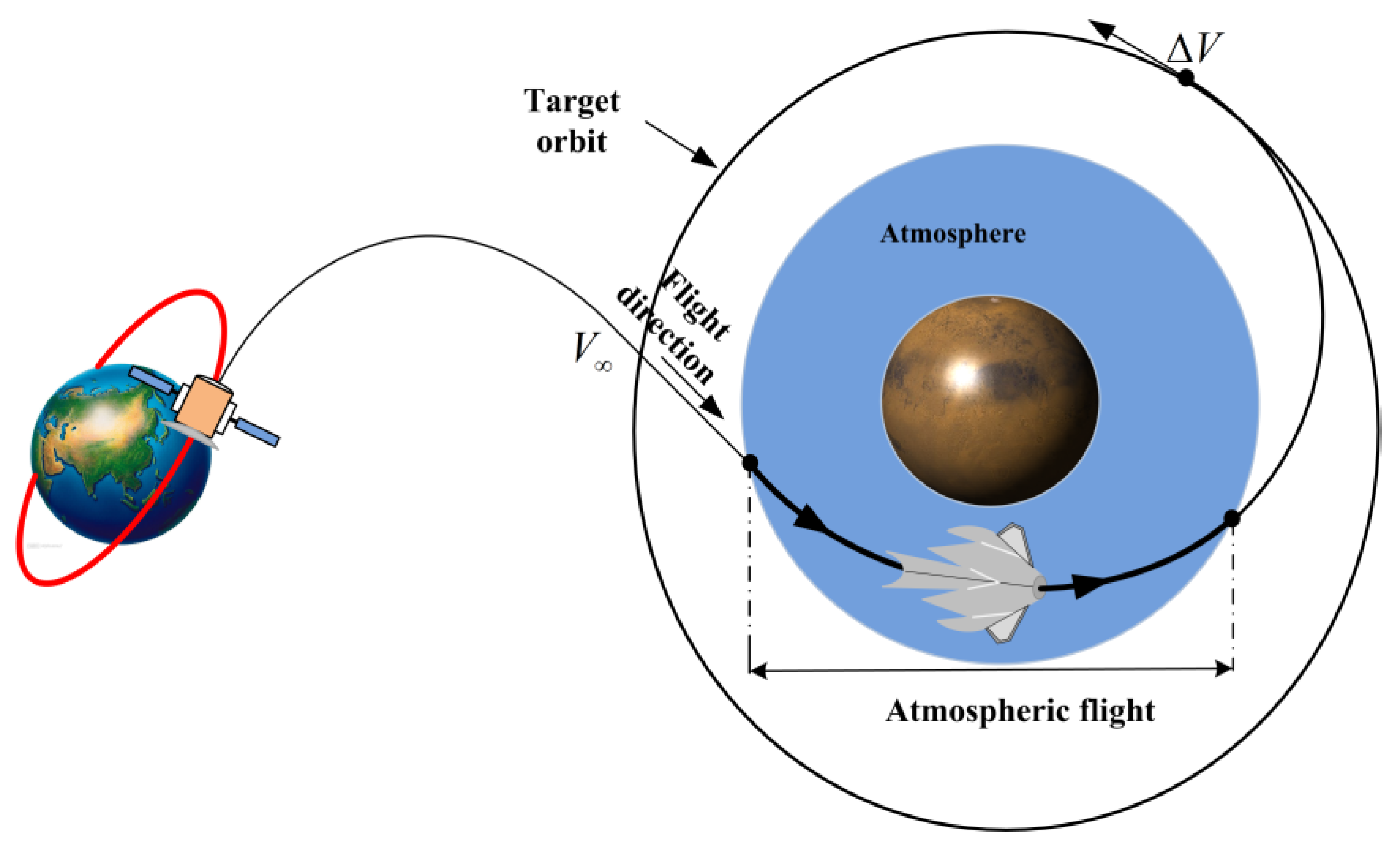
2.1. Aerocapture Process

As shown in Figure 1, the entire aerocapture process starts with the vehicle entering the atmosphere from a hyperbolic orbit; after completing atmospheric flight and flying out of the atmosphere, a single pulse maneuver is performed at the apoapsis to insert the vehicle into the target orbit.

2.2. Equation of Motion and Vehicle Model
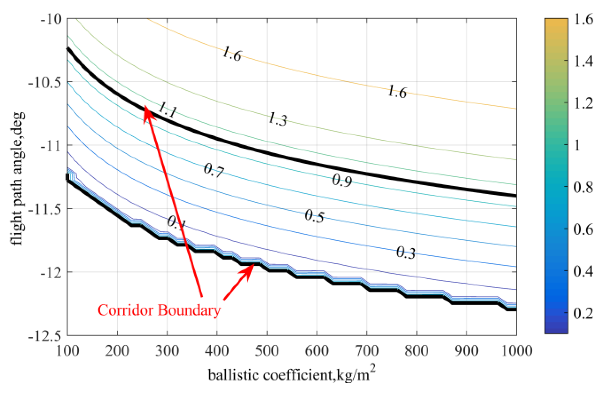
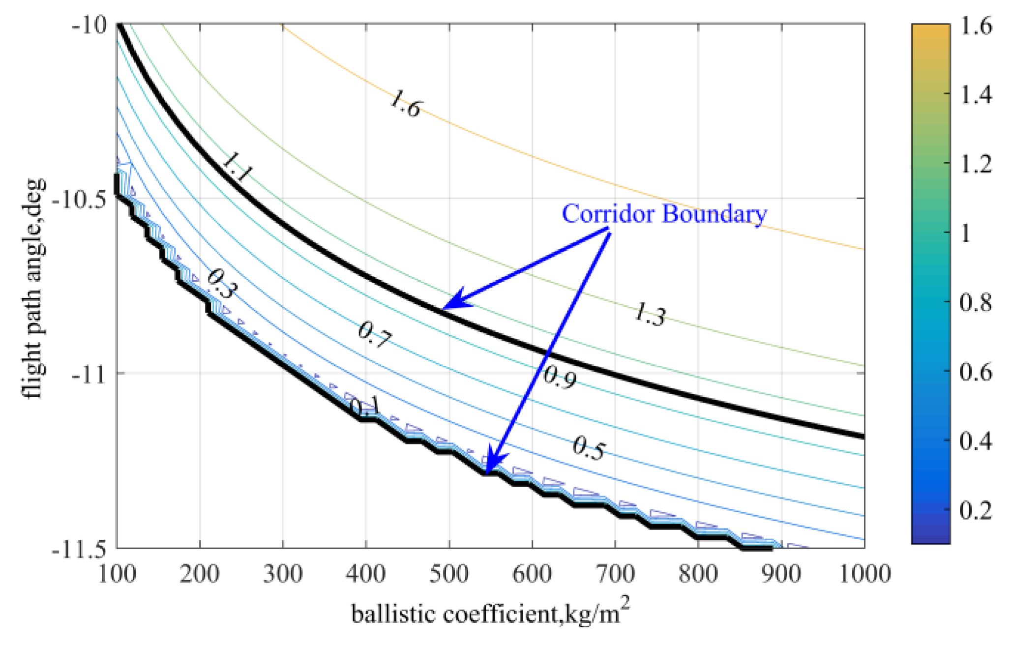
The atmospheric phase of Mars aerocapture is considered in this paper, and the motion of the vehicle is modelled as a point mass over a spherical nonrotating Mars. During the atmospheric flight, the vehicle is under the influence of gravity and the aerodynamic force. Thus, the differential equations of motion are given as [22].
d V d t = D m μ r 2 sin γ
d γ d t = L cos σ m V + ( V 2 r μ r 2 ) cos γ V
d ψ d t = L sin σ m V cos γ V r cos γ cos ψ tan ϕ
d r d t = V sin γ
d ϕ d t = V cos γ sin ψ r  
d θ d t = V cos γ sin ψ r cos ϕ
where the state vector is x = [ V , γ , ψ , r , ϕ , θ ] ; specifically, V is the velocity of the vehicle, γ is the flight path angle, ψ is the heading angle, r is the radial position and θ and ϕ are the longitude and latitude, respectively. σ is the bank angle, μ is the gravitational parameter and m is the mass of the vehicle. L and D are the lift and drag, respectively, and their specific forms are
{ L = 0.5 ρ V 2 S C L D = 0.5 ρ V 2 S C D
where 0.5ρV2 is the dynamic pressure, S is the reference area and C L and C D are the lift coefficient and the drag coefficient, respectively, which depend on the angle of attack, α . To make C L and C D invariable during atmospheric flight, α is always the given function of the Mach number, that is, the trim angle of attack. ρ is the Mars atmospheric density, for which an exponential model is applied, defined as follows
ρ = ρ 0 exp ( β h )
Finally, the specific values of spcific constants are shown in Table 1.

2.3. Corridor

The initial flight path angle plays an important role in the aerocapture maneuver, as its magnitude directly determines whether aerocapture is successful and, to a large extent, affects the size of the vehicle’s orbit after flying out of the atmosphere. The aerodynamic corridor intuitively indicates the value ranges of the initial flight path angle with the changes in the ballistic coefficient; when the initial flight path angle is within this range, the vehicle can be captured. The upper and lower bounds of the value range are the corridor boundaries. Thus, the orbital eccentricity after capture is chosen as a criterion, and only when the eccentricity is less than 1 can the aerocapture be completed successfully.
Figure 2 shows the aerocapture corridor when the vehicle has lift during atmospheric flight for an initial velocity of 6 km/s. The initial flight path angle and the ballistic coefficient jointly determine the corridor, and the initial flight path angle has a dominant influence on the corridor. In Figure 2, the value of the contour map is the orbital eccentricity out of the atmosphere. The two striking black and bold lines represent the corridor boundaries. The upper boundary line signifies the following: above this line, the vehicle will escape from Mars after the atmospheric flight, signifying that the aerocapture maneuver failed. In addition, the lower boundary line denotes that the vehicle will drop into Mars and not fly out of the atmosphere. The corridor trends show that the corridor width remains almost 1 deg, although the corridor boundary changes with the ballistic coefficient.
Figure 3 shows the aerocapture corridor considering no lift or a zero lift to drag ratio. This situation will appear when the deployable device is used for aerocapture. From the corridor boundary indicated by the black and bold lines, it can be seen that the corridor width is almost less than 0.5 deg. Since the corridor width to some extend characterizes the feasibility of aerocapture, when the corridor in Figure 3 is compared with the corridor in the premise of lift in Figure 2, it can be seen that lift modulation is more reliable than drag modulation.

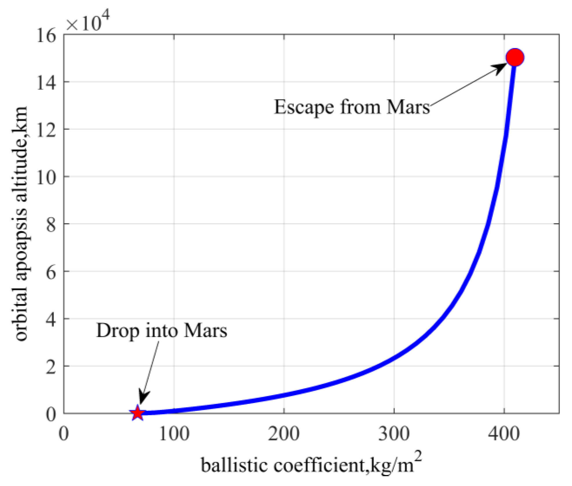
2.4. Influence of Ballistic Coefficient

The ballistic coefficient, an important variable for an aero-assisted vehicle, is defined as follows
B = m C D S
From Equation (9), we know that the ballistic coefficient is the ratio of mass to the product of the drag coefficient and reference area. Decreasing the ballistic coefficient substantially increases the drag force. The advantage of a deployable deceleration device is that the drag modulation system can greatly decrease the ballistic coefficient to increase the efficiency of aerocapture and achieve the capture of the vehicle to the target orbit while only requiring a single atmospheric flight. Figure 4 shows the influence of the ballistic coefficient on the target orbital altitude of apoapsis, which results in obvious changes ranging from hundreds of kilometers to almost millions of kilometers. Thus, varying the ballistic coefficient of the aero-assisted vehicle can promote the ability to control its energy depletion to efficiently capture the vehicle to any target orbit.
From the analysis in Section 2.3 and Section 2.4, it is clear that lift modulation can widen the aerocapture corridor and drag modulation can extend the target orbital range after aerocapture. Thus, the combination of lift modulation and drag modulation is very appealing. In other words, the joint lift and drag modulation flight control option can achieve complementary advantages.
The following sections of this paper will theoretically analyze the aerocapture processes under this flight control option and provide the optimal trajectories. It will demonstrate the feasibility and benefits of the joint modulation flight control option by analyzing the optimal aerocapture results, and the optimal trajectories will clearly illustrate the flight path in the Mars atmosphere under this flight control option. The analysis of the results will provide a reference for the establishment of the Mars aerocapture scheme and the design of the aerodynamic configuration of the aerocapture vehicle.

3. Optimal Aerocapture Problem Formulation

The aerocapture illustrated in Figure 1 is the controlled atmospheric flight process, and this section will present a detailed formulation of the optimal control problem. It should be noted that the joint flight control of lift and drag is determined by the optimal bank angle and reference area profiles.

3.1. Initial and Terminal Constraints

Aerocapture starts at the atmospheric edge, where the initial state variables are always certain, and the initial orbit is a hyperbola; thus, the initial conditions are given as
r ( t 0 ) = r 0 = h a t m + R M     γ ( t 0 ) = γ 0     V ( t 0 ) = V 0 ψ ( t 0 ) = ψ 0       θ ( t 0 ) = θ 0         ϕ ( t 0 ) = ϕ 0
where the initial heading angle, initial longitude and initial latitude are arbitrarily set to zero. One important issue to note here is that γ 0 should be negative to enable vehicle entry into the atmosphere. In addition, the terminal conditions and corresponding constraints are
              r f = h a t m + R M             γ f 0        
V f 2 2 μ e r f = μ 2 ( 2 r t r f 2 V f 2 cos 2 γ f μ r t 2 )
where r t is the apoapsis altitude of the target orbit. To ensure that the vehicle can fly out of the atmosphere, the terminal flight path angle must be positive. Because the vehicle should be inserted into the target orbit by only one burning, the apoapsis of the transfer orbit after atmospheric flight should equal the apoapsis of the target orbit, that is, the two orbits should be tangent in apoapsis.

3.2. Control Variables

To combine drag modulation and lift modulation, the control variables are the ballistic coefficient and bank angle. Assuming that the mass of the vehicle is unchanged during the entire aerocapture process, and the drag coefficient is a constant because of the trim angle-of-attack, the ballistic coefficient is directly determined by the reference area. Here, the reference area is simply chosen as a control variable to represent the ballistic coefficient; thus, the control variables must satisfy the following inequality constraints
S min S S max σ min σ σ max
where the upper and lower bounds of the control variables are given. To enable the optimization process to easily converge, based on experience, new control variables, u 1 , u 2 , are chosen to replace the reference area and bank angle, specifically, as
u 1 = S cos σ   ;   u 2 = S sin σ
σ = tan 1 u 2 u 1       ;       S = u 1 2 + u 2 2
Thus, the bounds of the new control variables will be reset as
S max u 1 S max   ;     S max u 2 S max
and to ensure that the optimal solution under the new control variables is equivalent to the original problem, an additional path constraint must be satisfied as follows
S min u 1 2 + u 2 2 S max

3.3. Path Constraints

The typical path constraints during atmospheric flight include the heating rate and load factor because the ability to endure the heating rate and load factor is limited; thus, such path constraints should be considered for aerocapture, and the specific constraints are [22]
Q = 9.4369 × 10 1 ( g 0 R M ) 3.15 ρ ( V g 0 R M ) 3.15 Q max
n = L 2 + D 2 m g 0 n max
The heating rate (unit: watts per square centimeter) of the stagnation point on the surface of the vehicle with a curvature radius of 0.3048 m, defined as Equation (18), is taken from Reference [20]; ρ is in kilograms per cubic meter, V has a unit of meters per second and the load factor is in g 0 . Note that Q max and n max are the heating rate limit and load factor limit, respectively.

3.4. Performance Index

The objective of this optimal control problem is to minimize the impulse used to insert the vehicle into target orbit (this impulse is hereinafter referred to as the insertion impulse), that is
J = 2 μ r b r t ( r t + r b ) r f r t V f cos γ f
where r b and r t are the periapsis and apoapsis of the target orbit, respectively, and the corresponding altitudes are h b and h t , respectively.

3.5. Optimal Control Problem

The complete form of the optimal control problem corresponding to Mars aerocapture is now stated as follows. The differential equations describing atmospheric flight are given in Equations (1) to (6). The state variables x = [ V , γ , ψ , r , ϕ , θ ] and the controls [ u 1 , u 2 ] are subject to the dynamic equations. The initial and terminal constraints are given in Equations (10)–(12), and the path constraints are given as Equations (17)–(19). The cost function is given as Equation (20).
For the optimal control problem, the direct method is currently widely used due to the development of computers and more robust performance. The hp-adaptive pseud-spectral method [21,22,23], one of the direct methods, performs better in terms of numerical precision and computing speed than other direct methods because of the adaptive meshing strategy, so it was to optimize the aerocapture trajectories. In this way, the optimal control problem was discretized into a nonlinear programming problem (NLP). The initial and terminal state variable constraints formulated in Equations (10)–(12) were added into constraint sets of the NLP. The control variable constraints given in Equation (16) were used as the upper and lower bounds of the control variables. The path constraints given in Equations (17)–(19) also has to be satisfied at each discrete point. Naturally, the performance index formulated in Equation (20) is the optimization objective of the NLP. In this research, the NLP was solved via the nonlinear programming problem solver SNOPT [24]. All computations were performed by MATLAB-R2016a.

4. Results and Analysis

In this section, the aerocapture trajectories were optimized based on lift and drag joint modulation. Considering different constraints and sizes in terms of the target orbit, the analysis of the results will reveal the benefit of such joint modulation. For Mars aerocapture, the initial state variables depend on the hyperbolic orbit because the orbital condition must be highly precise when the vehicle arrives at the edge of the Mars atmosphere; here, the initial states were not considered as variables. The vehicle completes the aerocapture maneuver through only a single atmospheric flight for all of the following optimization results. The initial state variables of the aerocapture are given in Table 2.

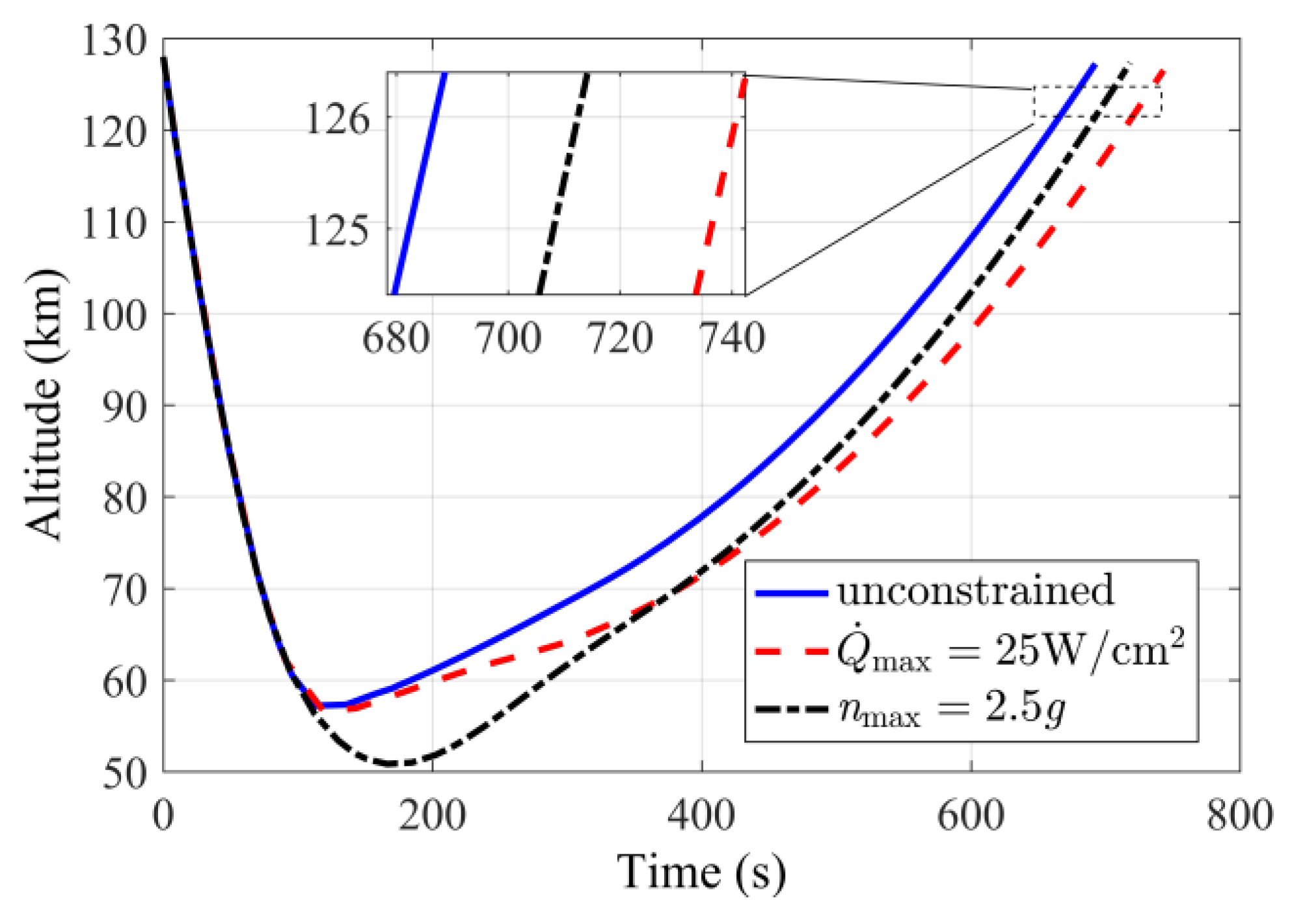
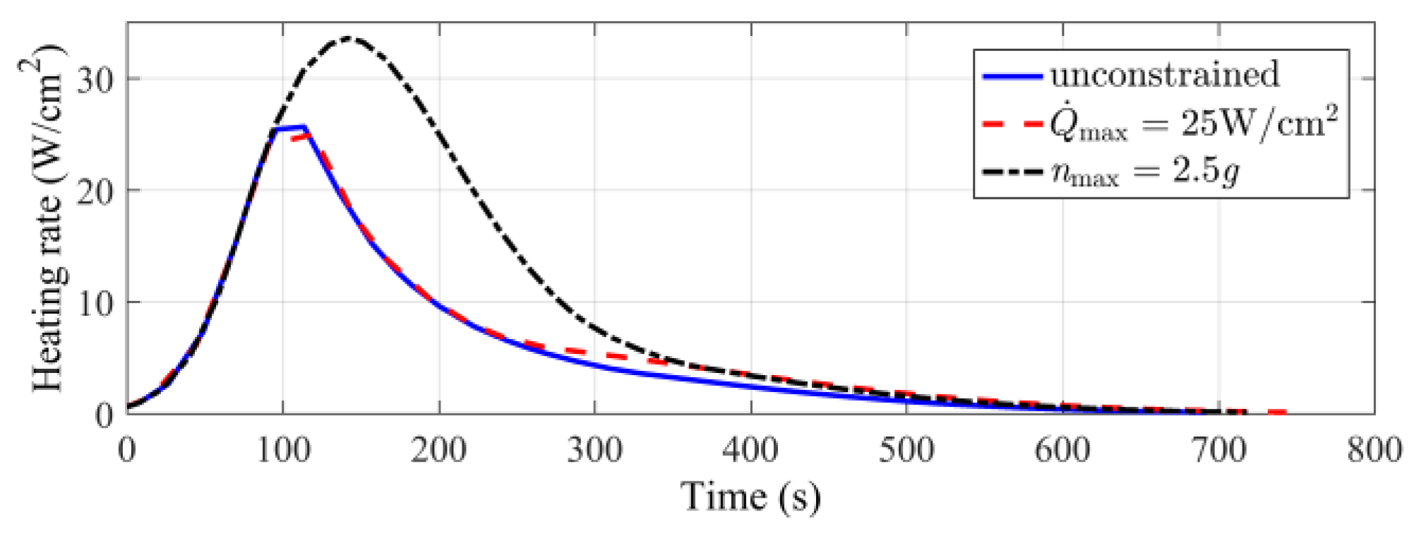
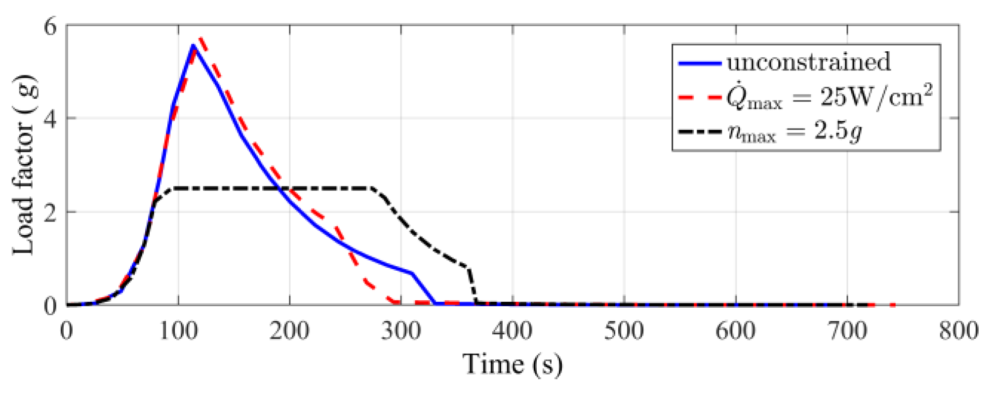
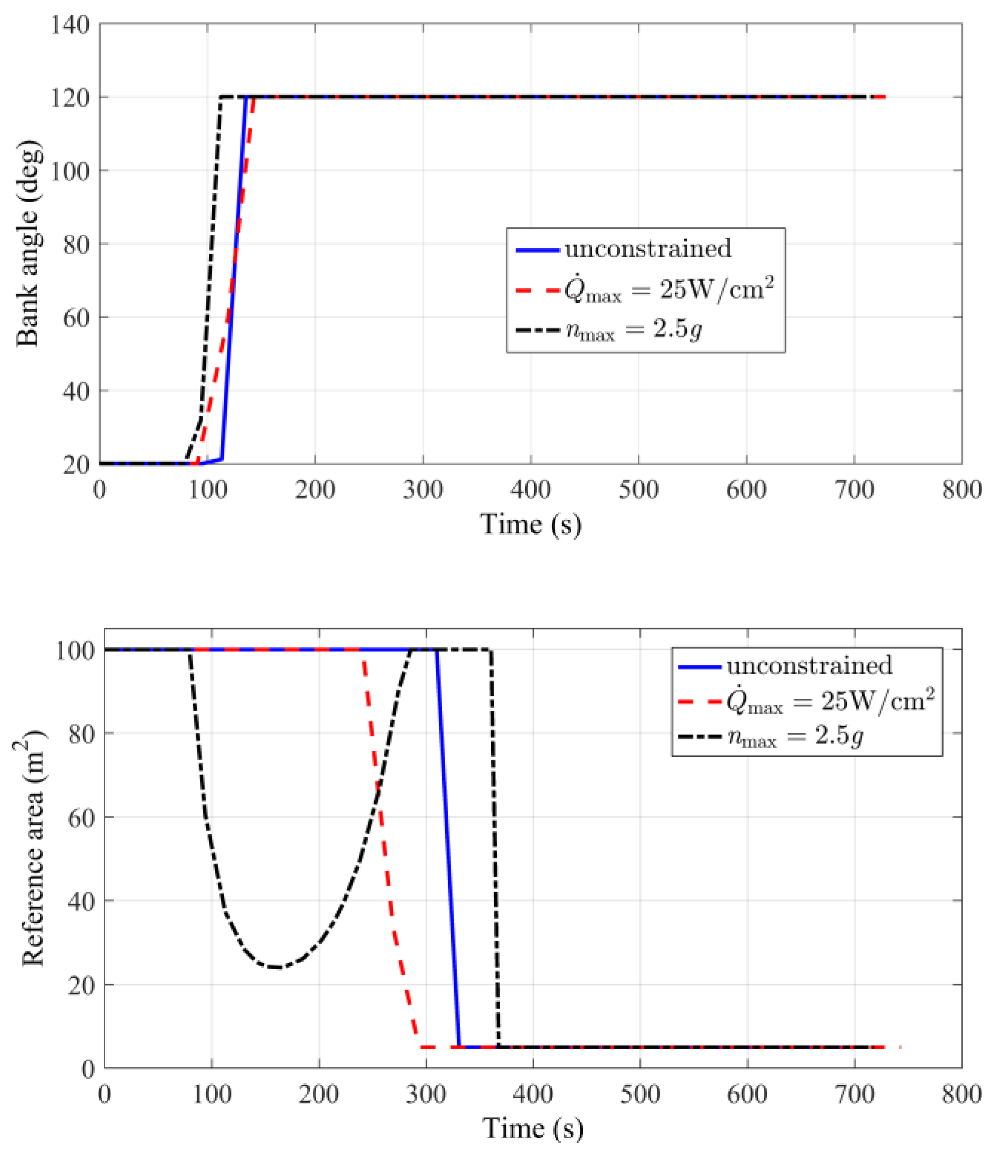
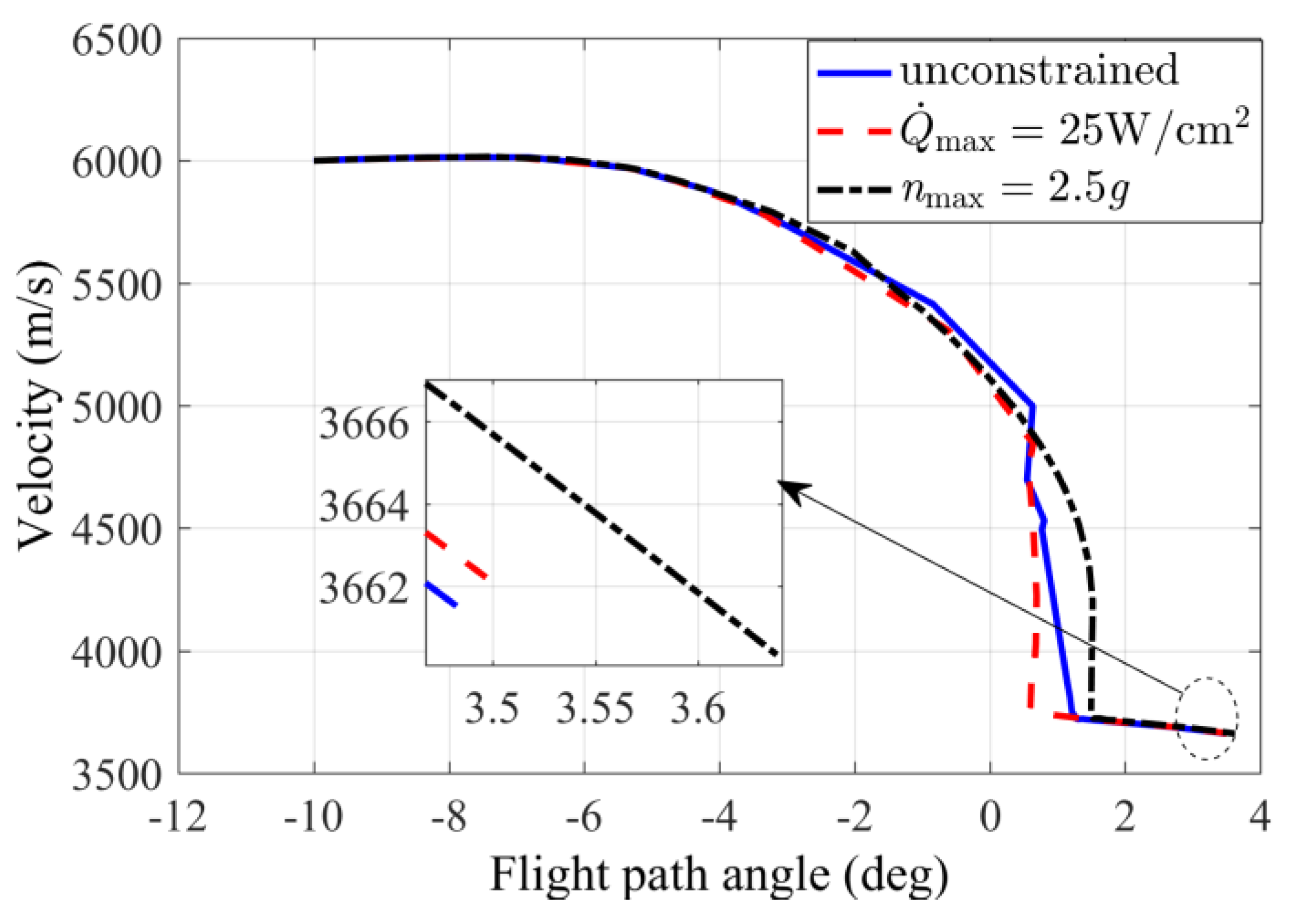
4.1. Influences of Path Constraint

The typical inequality trajectory path constraints formulated in Equations (18) and (19) during the atmospheric flight must be considered. Path constraints usually have a great impact on the optimal trajectories, so, here, the optimal results considering the different path constraints were analyzed. The initial state variables of the aerocapture remained as shown in Table 2. The height of the atmosphere edge h a t m was 128 km. The bounds on the magnitude of the reference area were set at S min = 5 and S max = 100 m2. The lower and upper bounds of the bank angle were σ min = 20 and σ max = 120 deg. The target orbit was considered as a circular orbit without loss of generality, so the altitude of the periapsis and the apoapsis of the target orbit were h t = 1000 and h b = 1000 km, respectively. The values of the limits of the path constraints were Q max = 25 W/cm2 and n max = 2.5( g 0 ), and values of the other variables and constants were the same as those stated in the above sections.
The altitude profiles during the atmospheric flight with different path constraints are plotted in Figure 5, in which the constraints of the heating rate and the load factor led to longer flight times, although the trajectories approximately overlapped at the initial entry phase (from the atmospheric initial edge to minimum altitude). Figure 6 shows the heating rate and the load factor profiles. Evidently, the peak heating rate is negligible because it is approximately 30 W/cm2, as proved in References [25,26,27]. Thus, as in the following sections, strict heating rate constraints were not imposed on the process of the atmospheric flight. However, the load factor constraint still had to be considered because the peak value was relatively high.
The bank angle and reference area histories are shown in Figure 7. The bank angle had a bang–bang structure, regardless of whether the path constraints were considered. A single step (momentarily switching from the minimum value to the maximum value) occurred at almost the same time for the unconstrained case, the heating rate constrained case and the load factor constrained case. The reference area also had a bang–bang structure, with only one switch under the unconstrained case and the heating rate-constrained case. However, it exhibited a singular segment (i.e., it was no longer a bang–bang structure but a continuously changing curve) for the load factor-constrained case, and this segment existed in the interval where the maximum value lay.
Figure 8 shows the velocity versus flight path angle profiles under different path constraints. Since the orbital size and the velocity at the apoapsis of the orbit out of atmosphere depend entirely on the terminal state variables (at the edge of the atmosphere) V f and γ f , as can be seen from the curves in Figure 8, all optimal trajectories would approximately overlap when the vehicle flies to the atmospheric exit, despite the flight times being slightly different, which indicates that the optimal V f and γ f for different path constraints were very close, with such terminal state variables directly determining the minimum orbit insertion burn. The results listed in Table 3 indicate that the impulse used to insert the vehicle into the target orbit is approximately 193 m/s, and when both heating rate and load factor constraints exist, the impulse consumption is slightly higher.

4.2. Impact of Control Variable Margins

During the atmospheric flight, the lift and drag subjected to the vehicle are modulated by control variables. For the joint modulation, the bank angle and the reference area are set as control variables. These two active control variables represent the flight control option, and the bounds of control variables determine the output control limit and the maneuverability of the vehicle. Therefore, it is necessary to analyze the influence of the bounds of the control variables on optimal aerocapture trajectories.

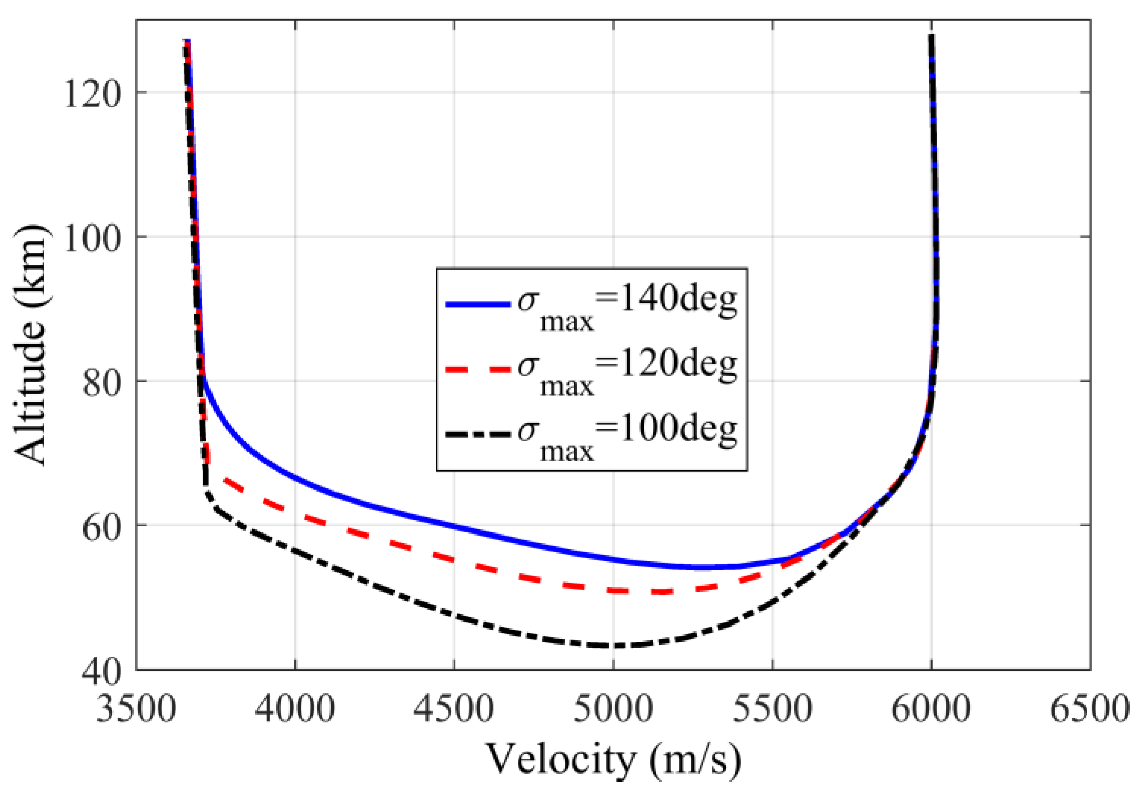
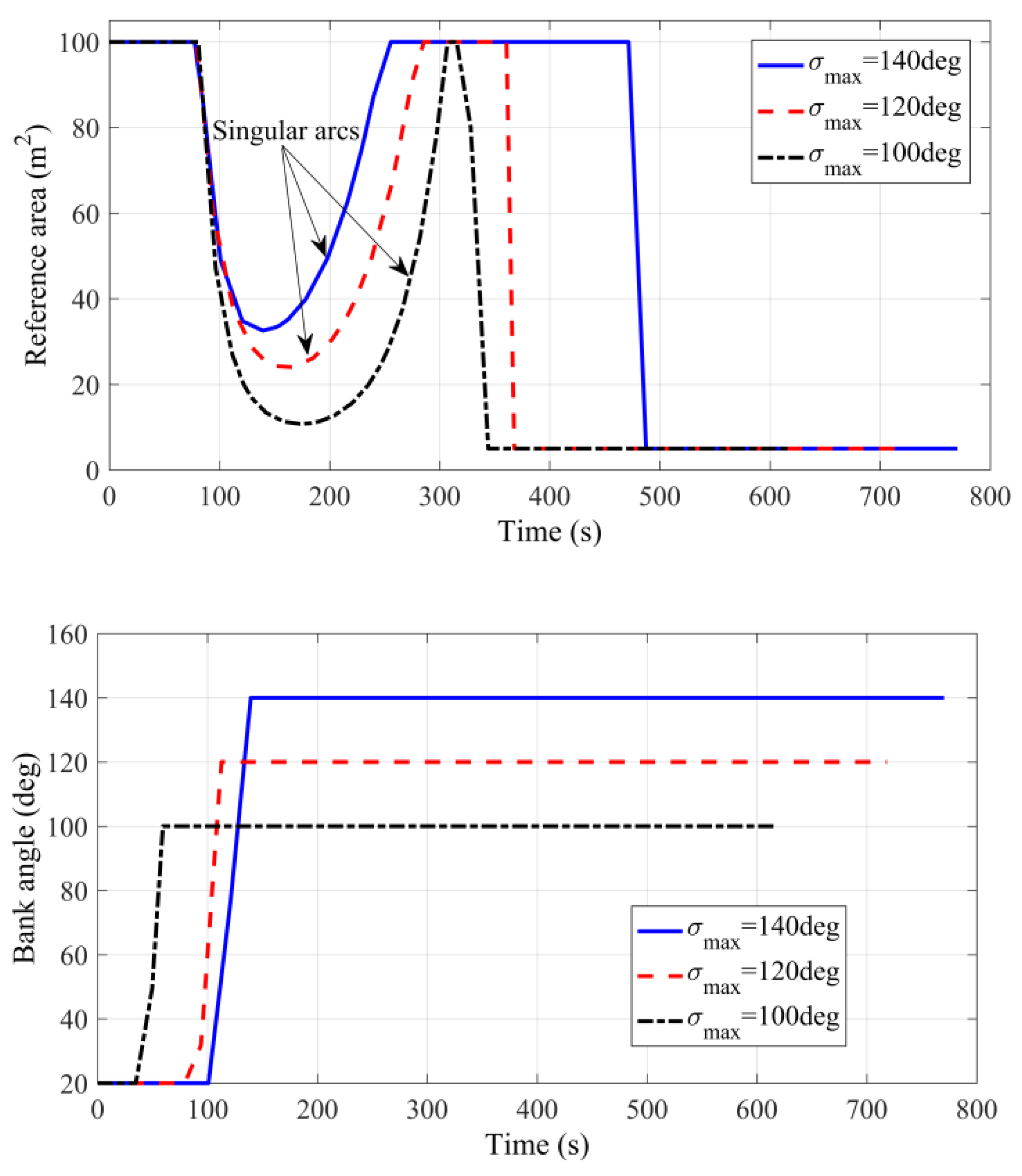
4.2.1. Upper Bounds of the Bank Angle

First comes the analysis of the impact of the bounds of the bank angle on the aerocapture trajectory. The regulating capability of the vehicle is directly determined by the upper bound of the bank angle, and it vastly affects the longitudinal control capability of the vehicle; thus, the effects of different maximum allowable bank angles on the optimal aerocapture trajectory were quantitatively analyzed. Three maximum bank angles, σ max = 140 deg, σ max = 120 deg and σ max = 100 deg, were chosen; the minimum bank angle remained unchanged.
Only the load factor constraint was considered. The heating rate constraint could be ignored because the peak heating rate does not need to be considered, as proved in the previous section. The load factor constraint was n max = 2.5 g 0 , where g 0 = 3.7137 m/s2 is the Mars gravitational acceleration at the Martian surface. Figure 9 shows the optimal trajectories with the different upper bounds in terms of the bank angle, the results of which indicate that σ max directly changes the aerocapture path and the flight range. When the upper bound of the bank angle σ max decreases, the flight altitude in the Mars atmosphere is relatively low, and the velocity at the minimum altitude is smaller, indicating that the velocity reduction in the descent phase is greater.
Figure 10 gives the reference area and bank angle histories with the different upper bounds of the bank angle. The decrease in σ max indicates that the vehicle flew at a relatively lower reference area during the entire atmospheric flight. According to Equation (1), the differential of the velocity was approximately proportional to 1 / r 2 , so the lower altitude necessarily promoted the decrease in the velocity. However, in order to minimize the insertion burn, the terminal velocity should be appropriate (not minimum). Hence, the drag D should be modulated to be smaller. As can seen from Equation (7), the drag can be reduced by reducing the reference area. Thus, from the altitude histories plotted in Figure 9 and the reference area histories plotted in Figure 10, the essence of this change can be revealed.
In addition, a large σ max causes the switch time of the bank angle to be advanced to maintain the maximum bank angle for a long time, which guarantees that the velocity reduction satisfies the terminal constraint given in Equation (12). The minimum insertion impulses, the peak path variables and the atmospheric flight times corresponding to the optimal results are given in Table 4. When σ max decreases, the minimum insertion impulses will clearly increase, especially for the case of σ max = 100 deg. Moreover, though the peak values of the heating rate and the load factor increase, the atmospheric flight time decreases to some extent because of the decrease in σ max .

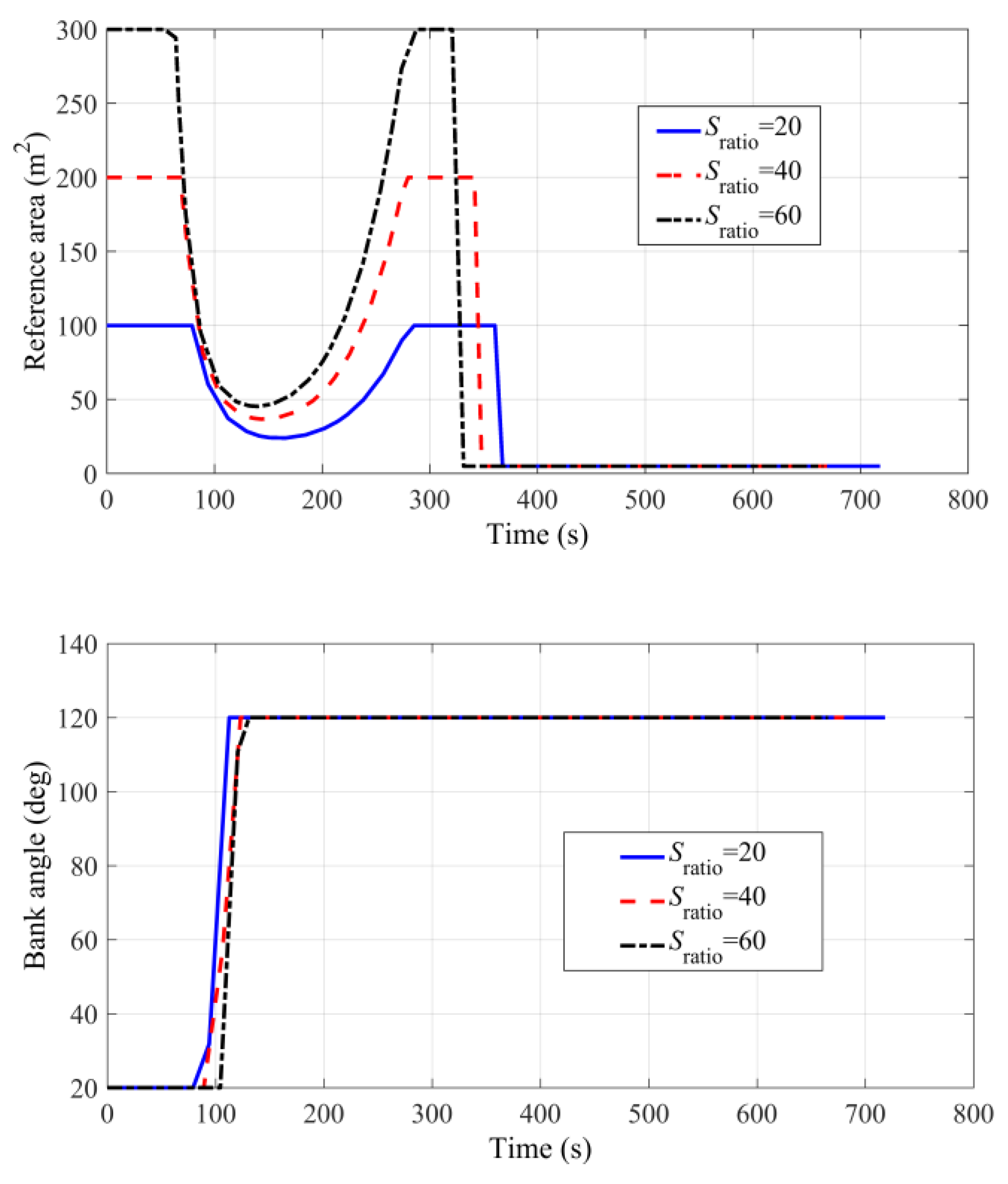
4.2.2. Reference Area Ratios

The ballistic coefficient is directly determined by the reference area, and the upper bound of the reference area is an indication of the maximum deployable ability or the minimum ballistic coefficient decrease via the expandable rigid wing of the vehicle; thus, the influence of the reference area on the optimal trajectory needs to be analyzed. Suppose that the lower bound of reference area S min is fixed (this assumption is indeed reasonable, because it represents that the expandable rigid wing of the vehicle is completely contracted) and that the upper bound of reference area S max is a multiple of the lower bound, that is, S r a t i o = S max / S min . The lower bound of the reference area S min = 5 m2, and the load factor constraint is n max = 2.5 g 0 . Three cases to consider are S r a t i o = 20 , S r a t i o = 40 and S r a t i o = 60 .
The data of minimum altitudes listed in Table 5 shows that a larger S r a t i o is found to lead to larger minimum altitude. As the reference area increases, the increase in the drag is inevitable. Therefore, the flight altitude should be relatively high in order to balance the rate of velocity reduction. Consequentially, the higher the S r a t i o , the higher the altitude curve during the atmospheric flight.
Additionally, it is obvious that the aerocapture effect is more beneficial for a larger S r a t i o . In addition, a larger S r a t i o decreases the peak heating rate and peak dynamic pressure simultaneously. Since increasing the S r a t i o can improve the vehicle’s ability to decelerate, the flight time is decreased and the insertion burn is reduced accordingly. Figure 11 gives the reference area and bank angle profiles with different S r a t i o . It is clear that a larger S r a t i o will make the switch time of the reference area decrease slightly, whereas the structures of the bank angle will remain nearly unchanged and will retain a bang–bang shape. Comparing Figure 10 with Figure 11, the bounds of the bank angle clearly affect the change in terms of the reference area, whereas the change in the bank angle is only marginally affected by the reference area ratios. Therefore, during the atmospheric flight of the aerocapture, the bank angle profile should be as fixed as possible.
The complete distributions of the minimum insertion impulse with different bounds in terms of the control variables are illustrated in Figure 12. When the upper bounds of both the bank angle and reference area ratios change, the minimum insertion impulse still has a similar distribution law, with the results listed in Table 4 and Table 5. It is noted that the upper bound of the bank angle plays a leading role in reducing the insertion impulse, and a smaller upper bound in terms of bank angle will lead to no solution.

4.3. Optimal Trajectories with Different Target Orbits

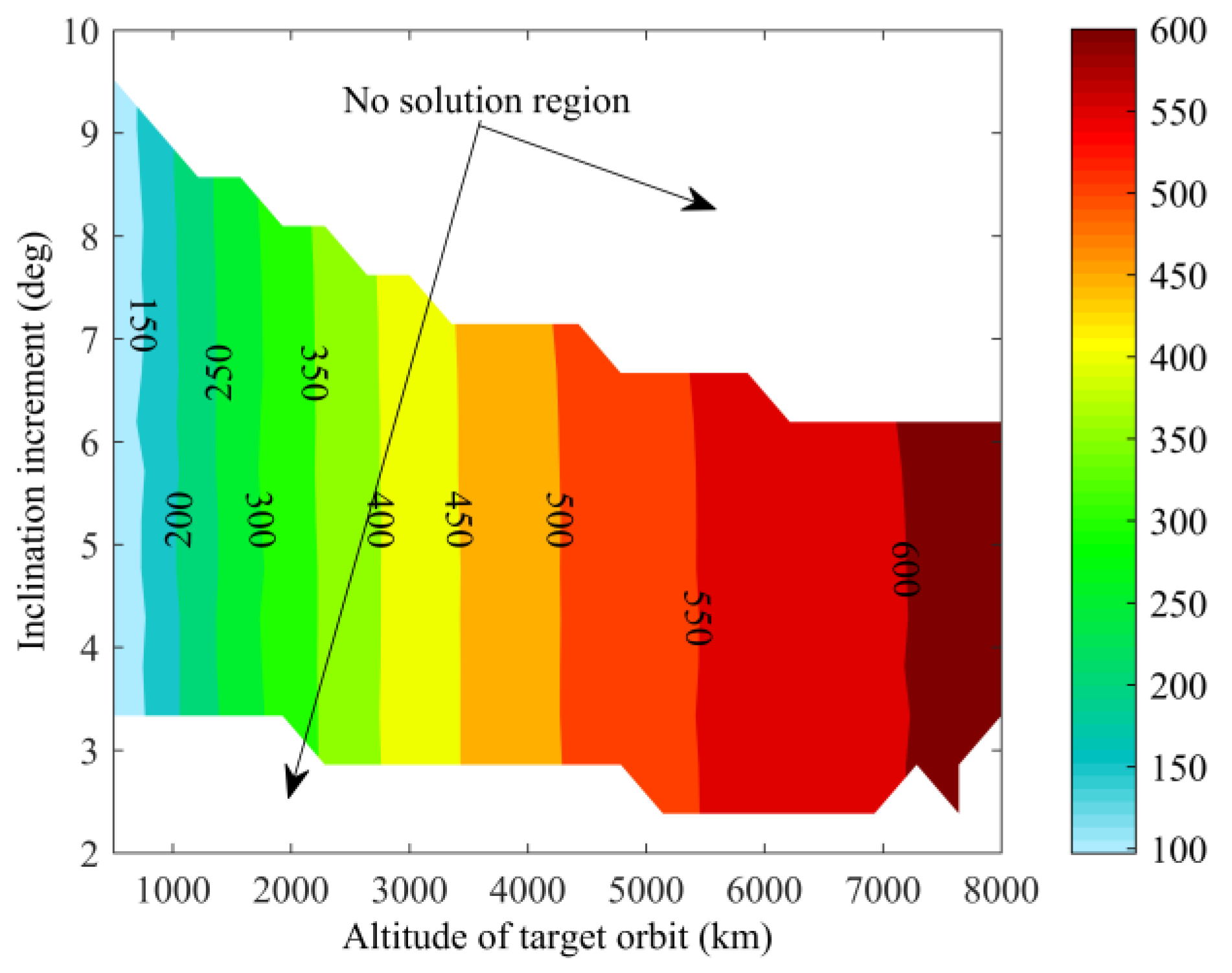
4.3.1. Different Target Orbit Altitudes

From Equations (12) and (20), the terminal constraints and the performance index are determined by the target orbit, i.e., they influence the optimal results and aerocapture trajectories. The target orbit is still considered to be a circular orbit. The influences of the altitudes of target orbits were analyzed under the assumption of a circular target orbit. The load factor constraint was n max = 2.5 g 0 . The flight trajectories with different altitudes of the target orbits are shown in Figure 13; when h t increases, the deceleration phase of aerocapture will become shorter, although the initial trajectories almost overlap. Table 6 lists the minimum insertion burns and specific parameters of atmospheric flight; the altitudes of the target orbit will not obviously affect the peak heating rates although the performance index increases, with the flight time evidently reducing when it increases.
Although the minimum insertion impulses are largely different, the peak heating rate and the load factor subjected to the vehicle are similar, which indicates that the descent phase is the main deceleration process, with the terminal constraint of the target orbit having little effect on the trajectory of the descent phase. However, the ascent phase during the atmospheric flight is largely affected by the altitude of the target orbit because in this flight phase, the trajectory will be modulated to satisfy the constraint in Equation (12), which is a necessary condition to realize the minimum insertion impulse.
Figure 14 shows the insertion burns with the different target orbits altitudes, indicating that higher target orbits require more impulses for inserting the vehicle. From the perspective of orbital energy, a higher target orbit has a larger energy difference relative to the transfer orbit after aerocapture.
Comparing the trajectory optimization results corresponding to different engine models in Section 3.2 and Section 3.3, the results of continuously variable parameters are more fuel-efficient because the thrust and specific impulse of Section 3.2 are greater than the values in Section 3.3 under the same input power.

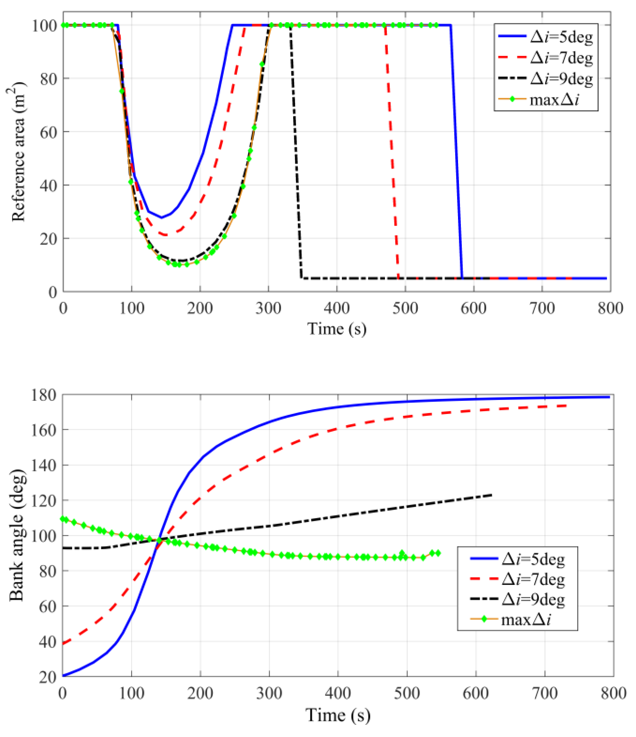
4.3.2. Different Inclination Increments

The inclination of the target orbit is always an orbital constraint for a specific Mars mission. Since changing the orbital inclination in space will consume a large amount of fuel using the purely propulsive maneuver, meeting the inclination of the target orbit will always be required during the atmospheric flight. The orbital inclination of the transfer orbit after the atmospheric exit is defined as
i f = arccos ( cos ψ f cos ϕ f )
where ψ f and ϕ f are the terminal heading angle and the terminal declination, respectively. The initial orbital inclination at the atmospheric interface is i 0 , and it was arbitrarily set to zero. Thus, the inclination increment was Δ i = i f i 0 = i f , which was the new constraint of the target orbit considered here. To analyze the maximum inclination increment in the atmosphere, an additional performance index J a = i f was considered, and the corresponding optimal solution is also shown in the last column in Table 6 and in the curves with green markers in Figure 15 and Figure 16. The maximum bank angle was σ max = 180 deg, and the load factor constraint was n max = 2.5 g 0 .
Table 7 shows the insertion burn, the peak path heating rate, the minimum altitude and the atmospheric flight time. With an increasing inclination increment, the insertion impulse and the atmospheric flight time will decrease, whereas the peak heating rate and the minimum altitude will, to some extent, increase. In addition, the maximum inclination increment that the vehicle can achieve during unpowered atmospheric flight is 9.181 deg.
The changes in inclination increments are shown in Figure 15, where the main change phase corresponds to the main deceleration phase. During the ascent phase, the inclination increment has little change, which also verified the fact illustrated in Section 4.3.1. That is, in this phase, the trajectory is modulated to satisfy the terminal altitude of the target orbit. Figure 16 shows the reference area and the bank angle profiles. The reference area still has a singular arc and a nonsingular arc, a continuously varying segment and a bang–bang segment. However, the bank angle continuously changes and is no longer a bang–bang structure because of the inclination increment constraint. When the inclination increment approaches the maximum inclination increment, the changing in the trend of the bank angle is relatively gentle, in the vicinity of 100 deg.
For aerocapture, sometimes both the altitude and inclination increment of the target orbit are required to be constrained. Figure 17 shows the minimum insertion impulse with different altitudes and inclination increments in terms of the target orbit. The insertion impulse is completely determined by the target altitude, but the inclination increment constraint largely limits the feasible region. Specifically, for a higher target altitude, the feasible region is smaller than the lower target altitude, which is because a shorter atmospheric flight time (as can be seen from Table 6) leads to less orbital plane maneuverability. Even so, for Mars aerocapture, such lift and drag joint modulation still has a large feasible region of target orbital constraint. Specifically, the feasible range of the target altitude is very wide, which is beneficial for the selection of the target orbit.
From the analysis above, the lift and drag joint modulation flight control options can greatly reduce the restrictions on the necessary conditions for Mars aerocapture. For different path constraints, control variable margins and target orbital constraints, the corresponding optimal solutions still exist. This fact indicates that such joint modulation can guarantee the existence of optimal trajectories under stringent constraints.
For pure drag modulation, the orbital plane constraint (such as the inclination increment constraint) surely cannot be met. For pure lift modulation, it is relatively difficult to satisfy the restricted target orbital constraint, with this being verified by a numerical simulation involving minimizing the apoapsis altitude of the orbit after aerocapture. When the condition is set as: σ min = 20, σ max = 160 deg and S = 10 m2, the minimum apoapsis altitude is 34,609.32 km, which means that the target orbit is never lower than this height and that it is only possible to choose a target orbit altitude higher than this value. Thus, from the contrasting analysis, the lift and drag joint modulation flight control option evidently extends the target orbital range after aerocapture, as visually demonstrated in Figure 17.

5. Conclusions

This work has proposed a flight control option with lift and drag joint modulation for Mars aerocapture and has revealed the feasibility and benefits of joint modulation through analyzing the corresponding optimal trajectories under different constraints. In the preliminary analysis for such a flight control option, Mars aerocapture corridors were contoured and the width of the corridor for lift modulation was found to be twice that for drag modulation. The results indicate that lift and drag joint modulation has potential complementary advantages. For different path constraints, the results show that the insertion impulse will increase on the condition of existing path constraints and that the heating rate constraint could be omitted for Mars aerocapture. Furthermore, control variable margins were found to clearly influence the optimal trajectories, although the insertion impulse was nearly unaffected. The bank angle continuously changes for different target orbital constraints and is no longer a bang–bang structure when the inclination increment constraint exists. In addition, if the inclination increment approaches the maximum inclination increment, the changing trend in terms of the bank angle is relatively gentle, in the vicinity of 100 deg. In contrast to pure lift modulation and drag modulation, the proposed flight control option relaxes constraints and extends target orbits.

Author Contributions

Conceptualization, Y.L. and H.H.; methodology, H.H.; software, G.S.; validation, Y.L., G.S. and H.H.; formal analysis, G.S.; investigation, H.H.; resources, G.S.; data curation, Y.L.; writing—original draft preparation, H.H.; writing—review and editing, Y.L.; visualization, G.S.; supervision, G.S.; project administration, H.H.; funding acquisition, Y.L. All authors have read and agreed to the published version of the manuscript.

Funding

This research was funded by the National Natural Science Foundation of China (Grant No. U20B2001).

Data Availability Statement

Not applicable.

Conflicts of Interest

The authors declare no conflict of interest.

References

  1. Parkinson, R.C. Why space is expensive-operational/economic aspects of space transport. Proc. IMechE. Part G J. Aerosp. Eng. 1991, 205, 45–52. [Google Scholar] [CrossRef]
  2. Gurley, J.G. Guidance for an aerocapture maneuver. J. Guid. Control. Dyn. 1993, 16, 505–510. [Google Scholar] [CrossRef]
  3. Wetzel, T.A.; Moerder, D.D. Vehicle/trajectory optimization for aerocapture at Mars. J. Astronaut. Sci. 1993, 42, 71–89. [Google Scholar]
  4. Miller, K.L.; Gulik, D.; Lewis, J.; Trochman, B.; Stein, J.; Lyons, D.T.; Wilmoth, R.G. Trailing Ballute Aerocapture: Concept and Feasibility Assessment. In Proceedings of the 39th AIAA/ASME/SAE/ASEE Joint Propulsion Conference and Exhibit, Huntsville, Alabama, 20–23 July 2003; pp. 2003–4655. [Google Scholar]
  5. Rohrschneider, R.R.; Braun, R.D. Survey of ballute technology for aerocapture. J. Spacecr. Rockets 2007, 44, 10–23. [Google Scholar] [CrossRef] [Green Version]
  6. Kozynchenko, A.I. Development of optimal and robust predictive guidance technique for Mars aerocapture. Aerosp. Sci. Technol. 2013, 30, 150–162. [Google Scholar] [CrossRef]
  7. Putnam, Z.R.; Braun, R.D. Drag-Modulation Flight-Control System Options for Planetary Aerocapture. J. Spacecr. Rocket. 2014, 51, 139–150. [Google Scholar] [CrossRef]
  8. Knittel, J.M.; Lewis, M.J. Concurrent aerocapture with orbital plane change using starbody waveriders. J. Astronaut. Sci. 2015, 61, 1–22. [Google Scholar] [CrossRef]
  9. Ai, Y.; Cui, H.; Zheng, Y. Identifying method of entry and exit conditions for aerocapture with near minimum fuel consumption. Aerosp. Sci. Technol. 2016, 58, 582–593. [Google Scholar] [CrossRef]
  10. Lyons, D.T.; Beerer, J.G. Mars global surveyor: Aerobraking mission overview. J. Spacecr. Rocket. 1999, 36, 307–313. [Google Scholar] [CrossRef] [Green Version]
  11. Smith, J.C.; John, C.; Bell, J.L. 2001 Mars Odyssey Aerobraking. J. Spacecr. Rocket. 2005, 42, 406–415. [Google Scholar] [CrossRef]
  12. Gladden, R.E. Mars reconnaissance orbiter: Aerobraking sequencing operations and lessons learned. Space Oper. Commun. 2009, 6, 1–10. [Google Scholar]
  13. Pontani, M.; Teofilatto, P. Post-aerocapture orbit selection and maintenance for the Aerofast mission to Mars. Acta Astronaut. 2012, 79, 168–178. [Google Scholar] [CrossRef]
  14. Lu, P.; Cerimele, C.J.; Tigges, M.A. Optimal Aerocapture Guidance. J. Spacecr. Rockets 2015, 38, 553–565. [Google Scholar]
  15. Haya-Ramos, R.; Blanco, G.; Pontijas, I.; Bonetti, D.; Freixa, J.; Parigini, C.; Bassano, E.; Carducci, R.; Sudars, M.; Denaro, A.; et al. The design and realization of the IXV Mission Analysis and Flight Mechanics. Acta Astronaut. 2016, 124, 39–52. [Google Scholar] [CrossRef]
  16. Cianciolo, A.M.; Davis, J.L. Entry, Descent and Landing Systems Analysis Study; NASA Technical Report; TM-2010-216720; NASA Langley Research Center: Hampton, VA, USA, 2010. [Google Scholar]
  17. Coustenis, A.; Atkinson, D.; Balint, T.; Beauchamp, P.; Atreya, S.; Lebreton, J.-P.; Lunine, J.; Matson, D.; Erd, C.; Reh, K.; et al. Atmospheric planetary probes and balloons in the solar system. Proc. IMechE Part G J. Aerosp. Eng. 2011, 225, 154–180. [Google Scholar] [CrossRef]
  18. Cianciolo, A.M.; Davis, J.L. Entry, Descent and Landing Systems Analysis Study; NASA Technical Report; TM-2011-217055; NASA Langley Research Center: Hampton, VA, USA, 2011. [Google Scholar]
  19. Dyke, R.E.; Hrinda, G.A. Aeroshell design techniques for aerocapture entry vehicles. Acta Astronaut 2007, 61, 1029–1042. [Google Scholar] [CrossRef] [Green Version]
  20. Girija, A.P.; Lu, Y.; Saikia, S.J. Feasibility and mass-benefit analysis of aerocapture for missions to Venus. J. Spacecr. Rocket. 2020, 57, 58–73. [Google Scholar] [CrossRef]
  21. Albert, S.W.; Schaub, H.; Braun, R.D. Flight Mechanics Feasibility Assessment for Co-Delivery of Direct-Entry Probe and Aerocapture Orbiter. J. Spacecr. Rocket. 2020, 59, 19–32. [Google Scholar] [CrossRef]
  22. Lu, P. Entry guidance: A unified method. J. Guid. Control. Dyn. 2014, 37, 713–728. [Google Scholar] [CrossRef]
  23. Rao, A.V.; Benson, D.A.; Darby, C.L.; Patterson, M.A.; Francolin, C.; Sanders, I.; Huntington, G.T. Algorithm 902: GPOPS, A MATLAB software for solving multiple-phase optimal control problems using the Gauss pseudospectral method. ACM Trans. Math. Softw. 2010, 37, 163–172. [Google Scholar] [CrossRef]
  24. Darby, C.L.; Hager, W.W.; Rao, A.V. Direct trajectory optimization using a variable low-order adaptive pseudospectral method. J. Spacecr. Rocket. 2011, 48, 433–445. [Google Scholar] [CrossRef]
  25. Darby, C.L.; Hager, W.W.; Rao, A.V. An hp-adaptive pseudospectral method for solving optimal control problems. Optim. Control. Appl. Methods 2010, 32, 476–502. [Google Scholar] [CrossRef]
  26. Gill, P.E.; Murray, W.; Saunders, M.A. SNOPT: An SQP algorithm for large-scale constrained optimization. SIAM J. Optim. 2002, 12, 979–1006. [Google Scholar] [CrossRef]
  27. Lockwood, M.K. Neptune aerocapture systems analysis. In Proceedings of the AIAA Atmospheric Flight Mechanics Conference and Exhibit, Providence, RI, USA, 16–19 August 2004. [Google Scholar]
Figure 1. Schematic diagram of the Mars aerocapture process.
Aerospace 10 00024 g001
Figure 2. Mars aerocapture corridor in the premise of lift.
Aerospace 10 00024 g002
Figure 3. The aerocapture corridor under pure drag modulation.
Aerospace 10 00024 g003
Figure 4. Orbital apoapsis altitude after aerocapture vs. ballistic coefficient.
Aerospace 10 00024 g004
Figure 5. Altitude profiles with different path constraints.
Aerospace 10 00024 g005
Figure 6. Heating rate and load factor profiles with different path constraints.
Aerospace 10 00024 g006aAerospace 10 00024 g006b
Figure 7. Bank angle and reference area profiles with different path constraints.
Aerospace 10 00024 g007
Figure 8. Velocity vs. flight path angle profiles with different path constraints.
Aerospace 10 00024 g008
Figure 9. Altitude vs. velocity histories with different upper bounds in terms of the bank angle.
Aerospace 10 00024 g009
Figure 10. Reference area and bank angle histories with different upper bounds in terms of the bank angle.
Aerospace 10 00024 g010
Figure 11. Reference area and bank angle with different reference area ratios.
Aerospace 10 00024 g011
Figure 12. Minimum insertion impulse (unit: m/s) with different upper bounds in terms of the bank angle and reference area ratios.
Aerospace 10 00024 g012
Figure 13. Altitude vs. velocity profiles with different target orbit altitudes.
Aerospace 10 00024 g013
Figure 14. Insertion velocity pulse vs. altitude of target orbit profiles.
Aerospace 10 00024 g014
Figure 15. Inclination profiles with different inclination increment constraints.
Aerospace 10 00024 g015
Figure 16. Optimal control variables with different inclination increment constraints.
Aerospace 10 00024 g016
Figure 17. Minimum insertion impulse (unit: m/s) with different altitudes and inclination increments in terms of the target orbit.
Aerospace 10 00024 g017
Table 1. The physical constants.
ParameterValueUnit
Gravitational parameter μ42,828m3/s2
Atmospheric density of the surface of Mars ρ00.01474kg/m3
Atmospheric density coefficient β1/8805.7m−1
Mass of the vehicle m2000kg
Mars radius RM3396km
Maximum altitude of sensible atmosphere hatm128km
Lift coefficient of the vehicle CL0.4--
Drag coefficient of the vehicle CD1.2--
Table 2. Initial state variables.
Parameterr0(km) V 0 ( m / s ) γ 0 ( ° ) ψ 0 ( ° ) θ 0 ( ° ) ϕ 0 ( ° )
Value35246000−10000
Table 3. Insertion impulses for different path constraints.
Path ConstraintsInsertion Impulses (m/s)
No constraints192.14
Heating rate constraint193.27
Table 4. Optimal results with different upper bounds in terms of the bank angle.
Upper Bounds of the Bank Angle σmax (deg)Minimum Insertion Impulses J (m/s)Peak Heating Rates (W/cm2)Peak Dynamic Pressures (KN/m2)Atmospheric Flight Times (min)Minimum Altitudes (km)
σmax = 140°190.94730.8690.45112.83954.14
σmax = 120°193.49633.6120.61111.97150.83
σmax = 100°200.45747.3441.36410.26843.36
Table 5. Optimal results with different reference area ratios.
Reference Area Ratios, SratioMinimum Insertion Impulses J, m/sPeak Heating Rates, W/cm2Peak Dynamic Pressures, KN/m2Atmospheric Flight Times, minMinimum Altitudes, km
Sratio = 20190.94730.8690.45112.83950.83
Sratio = 40193.49633.6120.61111.97154.69
Sratio = 60200.45747.3441.36410.26856.63
Table 6. Optimal results with different reference area ratios.
Altitude of Target Orbit ht, kmMinimum Insertion Impulses J, m/sPeak Heating Rates, W/cm2Peak Dynamic Pressures, KN/m2Atmospheric Flight Times, min
ht = 50102.09734.9770.68215.196
ht = 3000419.95431.3730.5028.7498
ht = 5500552.49230.7900.4567.6179
ht = 8000615.79730.7240.4357.0521
Table 7. Optimal results with different inclination increment constraints.
Inclination Increment Δi, degMinimum Insertion Impulses J, m/sPeak Heating Rates, W/cm2Peak Dynamic Pressures, KN/m2Atmospheric Flight Times, min
Δi = 5189.96132.78952.75813.242
Δi = 7190.59736.29050.07812.392
Δi = 9198.49046.09644.12010.389
Δi = 9.181 (max)207.03649.19242.8749.0864
Disclaimer/Publisher’s Note: The statements, opinions and data contained in all publications are solely those of the individual author(s) and contributor(s) and not of MDPI and/or the editor(s). MDPI and/or the editor(s) disclaim responsibility for any injury to people or property resulting from any ideas, methods, instructions or products referred to in the content.

