Article

Numerical Simulation and PIV Experimental Investigation on Underwater Autorotating Rotor

1
School of Aeronautic Science and Engineering, Beihang University, Beijing 100191, China
2
Institute of Unmanned System, Beihang University, Beijing 100191, China
3
Shanghai Aircraft Design & Research Institute, COMAC, Shanghai 201210, China
*
Author to whom correspondence should be addressed.
Aerospace 2023, 10(1), 20; https://doi.org/10.3390/aerospace10010020
Submission received: 17 November 2022 / Revised: 21 December 2022 / Accepted: 21 December 2022 / Published: 25 December 2022

Abstract

:
In this work, the flow field of an autorotating rotor in a water tunnel with various pitches and shaft backward angles was investigated via particle image velocimetry (PIV). The experiments were carried out on a free-rotating two-bladed single rotor. Computational Fluid Dynamics (CFD) based on moving overset grids were developed to study the hydrodynamic characteristics of an underwater autorotating rotor. The simulation results are in good agreement with the test results. The thrust and thrust coefficient of the underwater autorotating rotor were calculated by CFD simulation under different situations. The research demonstrates that rotational speed and thrust have a significant positive correlation with water velocity, pitch, and shaft back angle. In particular, the thrust coefficient scarcely varies with the shaft backward angle. An underwater autorotation rotor with a thin airfoil, negative torque, and a suitable number of blades can increase the thrust and thrust coefficient. The investigation is of significance in enriching the autorotation theory of rotors and helping to develop underwater autorotating rotors.

1. Introduction

Underwater vehicles are playing an important role in marine resource exploration and marine environmental investigation [1,2]. At present, the majority of underwater vehicles require power to provide propulsion for navigation [3]. It is important to develop an underwater vehicle that achieves long-time unpowered navigation with thrust provided by an autorotating rotor.
Autogiro is a mature aircraft. It has wide prospective applications in the future [4,5]. The autogiro was developed by Juan de la Cierva [6,7] in the 1920s, who introduced the mature age of rotorcrafts. Leishman [8,9] introduced the development history of rotorcraft in detail. Most of the research on autorotation was conducted in the early 20th century. Glauert [10] proposed a theory of autorotorcraft based on simplified assumptions, which established the basic theory for investigating the aerodynamic characteristics of autorotorcraft. Wheatley [11,12,13,14,15,16,17] carried out a lot of research on autorotorcraft. A scaled-down model of the VPM M16 rotorcraft was tested in a wind tunnel at Glasgow University, UK. Houston [18,19,20,21,22,23] investigated the advantages and disadvantages of this rotorcraft design scheme, the system identification technique, the maneuvering stability characteristics, the flight dynamics characteristics, and the flight quality. Bagiev [24,25,26] validated the mathematical simulation model of the rotorcraft in terms of leveling and maneuvering response by comparing numerical calculations with experimental results.
However, most of the research is mainly focused on autogiro in air, and less research has been done on autorotating rotors. With the development of technology, the performances of autorotation rotors can be better demonstrated. The autorotation state of the rotor can also be applied underwater, making so-called autonomous underwater vehicles [27,28,29], which is another meaning for this water tunnel experiment.
Particle image velocimetry (PIV) is a very mature technique developed in the 1970s, specializing in investigating flow features quantitatively [30,31]. For the helicopter rotor field, Yu et al. investigated the induced velocity and flow feature of the coaxial rotor in hovering and forward flight conditions in a water tunnel via PIV [32,33,34]. They compared the flow feature of coaxial rotors with single rotors in detail. With three-component PIV development, the flow features of full-equipped helicopters can be comprehensively investigated with multiple planes of observation windows [35,36,37].
Computational Fluid Dynamics (CFD) is a very mature technique developed in the 1960s, specializing in the flow field. Its advantages are low cost, short cycle time, and high accuracy. Many advanced CFD techniques have been used in the numerical simulation of helicopter rotors [38,39,40]. In particular, the overset grid technique [41,42,43,44,45,46,47,48] has been widely used in helicopter rotor simulation, and the method has been employed for various operating conditions such as hovering, forward flight, vertical flight, and near-ground flight of helicopters. PIV tests and CFD calculations for underwater rotorcraft are scarce [49]. Most of the studies have been conducted on rotorcraft flying in the air. Kim et al. [50] used computational fluid dynamics (CFD) for the numerical simulation of a six-degree-of-freedom (6DOF) free-running maneuver of an underwater vehicle. Dantas et al. [51] analyzed the hydrodynamic efforts generated on an AUV considering the combined effects of the control surface deflection and the angle of attack using CFD software based on the Reynolds-averaged Navier–Stokes formulations. Kilavuz et al. [52] conducted a numerical and experimental study of the flow characteristics of an unmanned underwater vehicle (UUV) with the commonly used Myring profile using computational fluid dynamics and particle image velocimetry techniques. Gao et al. [53] estimated the drag on an autonomous underwater vehicle (AUV) and optimized the shape using CFD. Hong et al. [54] conducted a numerical study of the hydrodynamic performance of a portable autonomous underwater vehicle (AUV). Current research on underwater vehicles is mainly focused on powered UAVs. There is a shortage of research on UAVs that rely on rotor autorotation to provide thrust and achieve unpowered navigation. In the future, unpowered underwater autorotates can be used for undersea mapping and military reconnaissance. Consequently, there is an enormous requirement to conduct experimental research and simulation analysis on underwater autorotating rotors.
The purpose of the paper is to investigate the hydrodynamic characteristics of the underwater autorotating rotor. Both an experimental and a numerical study have been performed. The rotational speed and flow field of the autorotating rotor was investigated in a water tunnel via the particle image velocimetry (PIV) technique. A three-dimensional overset grid numerical simulation was conducted on an underwater autorotating rotor. The test results were compared with the simulation data to validate the CFD simulations. The effect of water velocity, shaft backward angle, pitch, twist angle, airfoil, and blade number on the thrust and thrust coefficient was presented in detail.

2. Experiment Setup

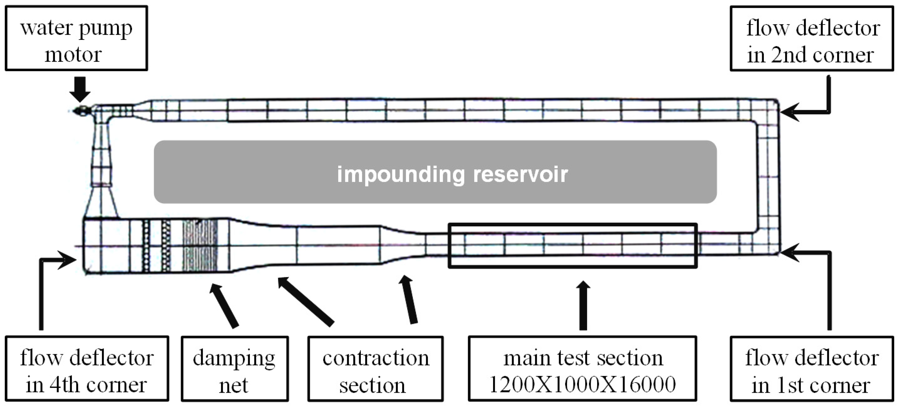
2.1. Water Tunnel and Rotor System

The experiments were carried out in the low-speed water tunnel of the Key Laboratory of the Ministry of Education at Beihang University. As shown in Figure 1, the water tunnel was in a closed loop form, which had a main test section of 1.2 × 1.0 × 16   m 3 with a turbulence intensity of 0.3 % . The walls of the test section were made of glass with good light transmission. The maximum velocity of the test section was approximately 0.366   m / s and the minimum velocity was 0.1   m / s . The testing water temperature was 20   .
The main part of the rotor system was a two-blade single rotor. The rotor was able to rotate freely in the clockwise direction (seen from above), and its rotational speed was recorded by a flange plate fixed on the rotation shaft that shaded a photoelectric switch fixed to the base. The photoelectric switch recorded the accurate time when the blade rotated to a specific phase position, which was an important reference of wake age. Each blade was untwisted and rigid and was connected rigidly to the hub. The rotor had a radius R = 0.25   m , with a blade root cutout of 0.053   m ( 21 % of rotor radius). The blade had a rectangular planform and a chord of 0.025   m . The airfoil was NACA 0015. The surface of the blades was painted black for reducing reflection. In the rotor system, there were two variable parameters. One was the pitch, the other was the shaft backward angle. The shaft backward angle could be changed from 60 ° to 60 ° . The detailed rotor properties are shown in Table 1.

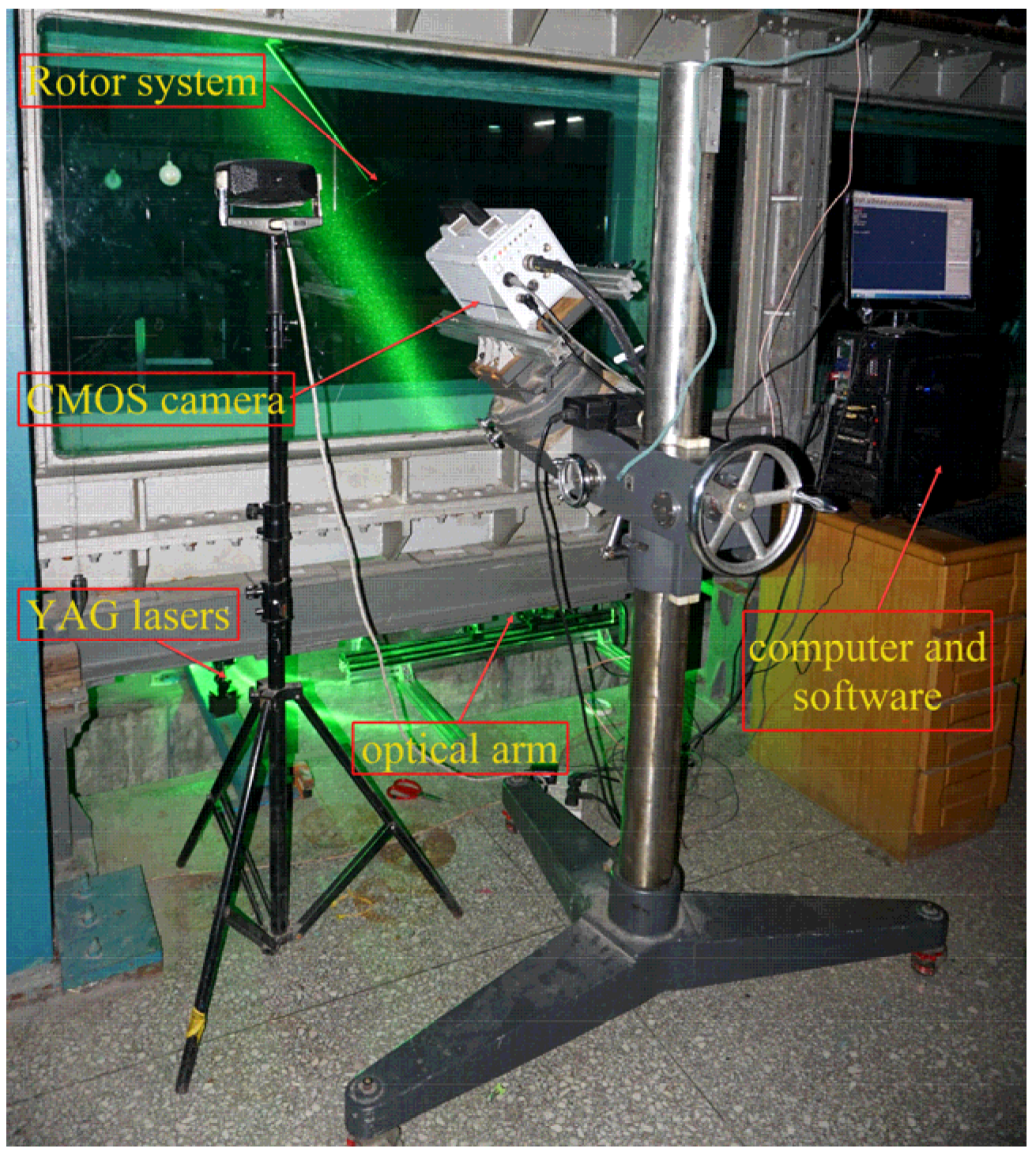
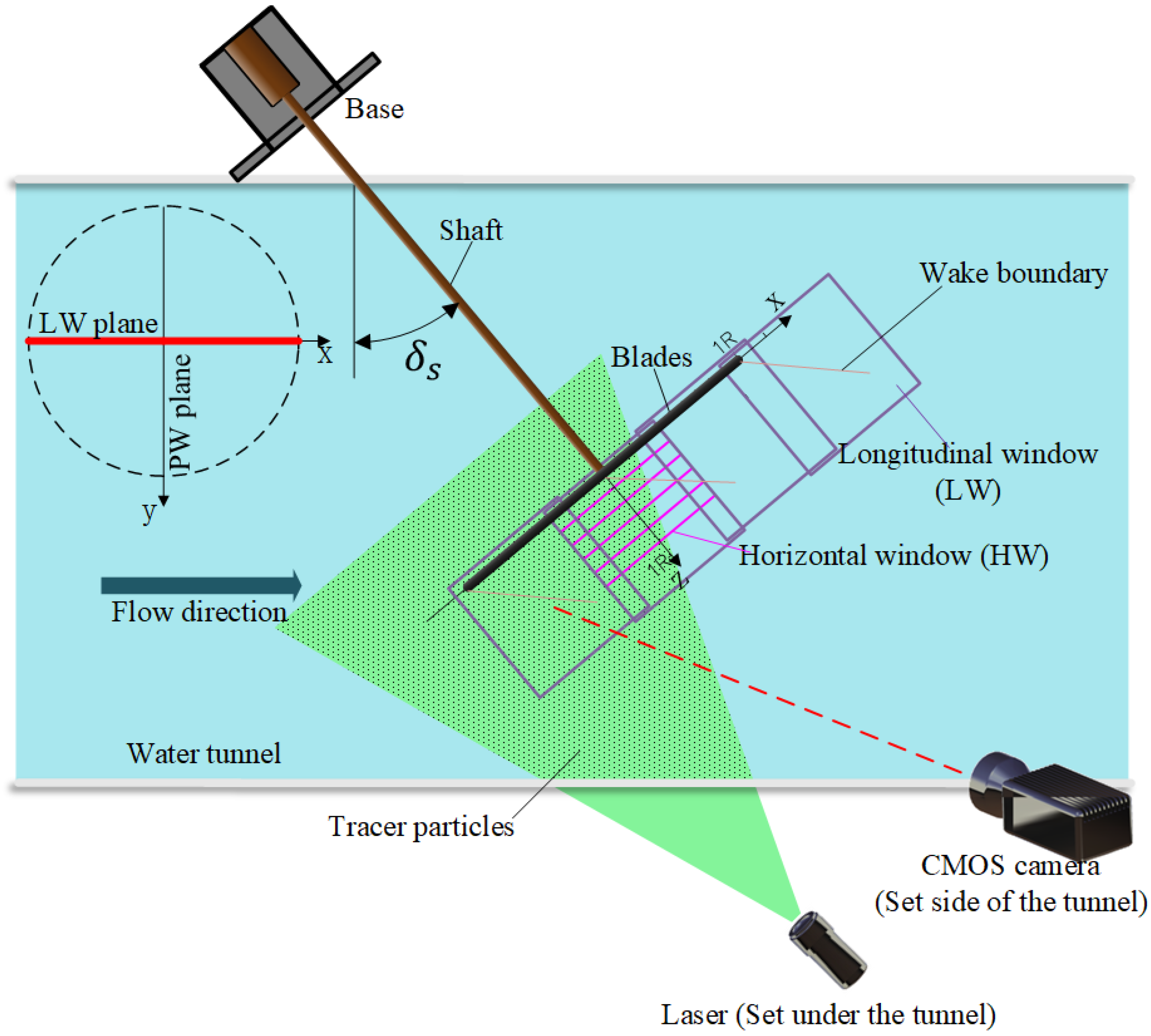
2.2. PIV Instrumentations

Figure 2 shows the entire PIV system and the rotor setup configuration. The complete system consisted of a pair of frequency-doubled Nd: YAG lasers, an optical arm, light-sheet optics, a digital CMOS camera of 2048 × 2048 pixels resolution, a high-speed frame grabber, image acquisition and analysis software, and a computer. The fiber optic light arm transmitted the laser light from the dual Nd: YAG lasers to the rotor flow field. The lasers lighted an observation plane in the wake, by emitting a 1 mm thickness light sheet.
As shown in Figure 3, the longitudinal observation planes were determined by the shaft axes and the flow direction. The longitudinal plane contained the longitudinal window (LW). The observation planes obtained a spatial view of the flow field, which got a clear comprehension of the autorotation mechanism. The CMOS camera captured images of the flow field from a direction perpendicular to the observation plane lit by the laser sheet.
In Figure 3, δ s means the shaft backward angle. It is a very important parameter of the autorotation that could influence the rotational speed greatly. The blade’s pitch angle θ could also be changed. A positive θ means that the blade’s leading edge rotated downward direction to the bottom of the water tunnel, while a negative θ means that the blade leading edge is rotated in an upward direction toward the surface of the water tunnel. This is to say, the device was placed upside down in the water tunnel, which has the advantage of avoiding the flow feature being disturbed by the rotating shaft.

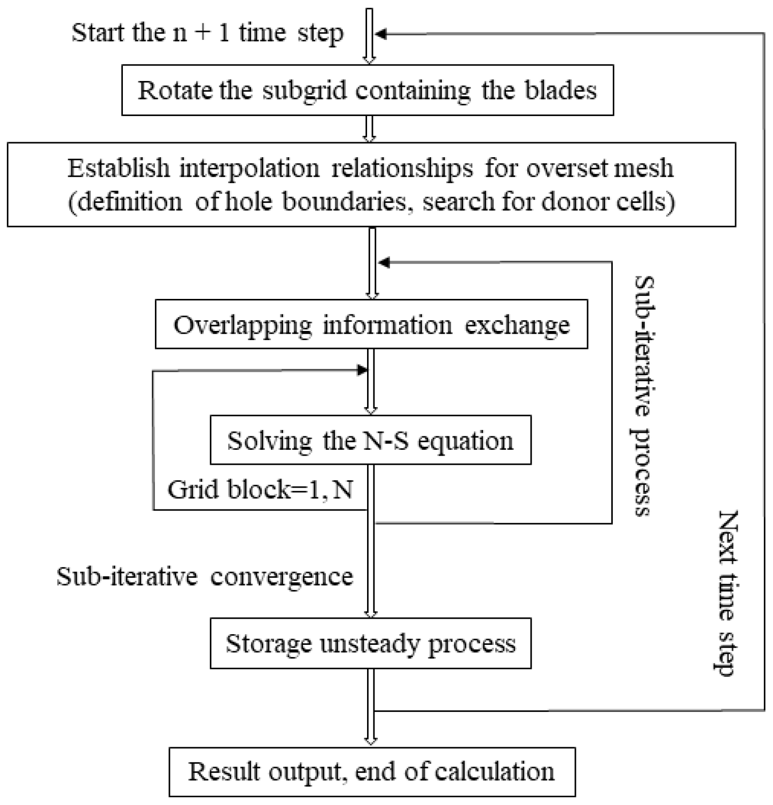
3. CFD Simulation Method

3.1. Governing Equation and Solution Method

The conserved Reynolds averaged Navier–Stokes equation [55] of three-dimensional, viscous, unsteady, and compressible flow in the inertial coordinate system can be obtained as:
t V W d V + S ( F c F v ) · n d S = 0
where W = [ ρ , ρ u , ρ v , ρ w , ρ e ] T is a conserved variable, F c = ( f , g , h ) is the convective flux, and F v = ( a , b , c ) is the viscous flux. The specific expression is:
f = [ ρ u ρ u 2 + p ρ u v ρ u w ρ u e + u p ] ,   g = [ ρ v ρ u v ρ v 2 + p ρ v w ρ v e + v p ] ,   h = [ ρ w ρ u w ρ v w ρ w 2 + p ρ w e + w p ]
a = [ 0 τ x x τ y x τ z x u τ x x + v τ y x + w τ z x q x ˙ ] b = [ 0 τ x y τ y y τ z y u τ x y + v τ y y + w τ z y q y ˙ ] c = [ 0 τ x z τ y z τ z z u τ x z + v τ y z + w τ z z q z ˙ ]
In the viscous flux, the stress can be expressed as follows:
{ τ x x = 2 ( μ l + μ t ) [ u 1 3 ( u + v + w ) ] τ y y = 2 ( μ l + μ t ) [ v 1 3 ( u + v + w ) ] τ z z = 2 ( μ l + μ t ) [ w 1 3 ( u + v + w ) ] τ x y = τ y x = ( μ l + μ t ) ( u + v ) τ y z = τ z y = ( μ l + μ t ) ( v + w ) τ z x = τ x z = ( μ l + μ t ) ( w + u )
where, μ l is laminar viscosity coefficient, μ t is turbulent viscosity coefficient, u , v ,   w is velocity in x , y , z direction.
The heat flow in x , y , z direction can be expressed as follows:
{ q ˙ x = γ R γ 1 ( μ l P r l + μ t P r t ) T x q ˙ y = γ R γ 1 ( μ l P r l + μ t P r t ) T y q ˙ z = γ R γ 1 ( μ l P r l + μ t P r t ) T z
The relationship between temperature and pressure can be expressed as follows:
p = ρ ( γ 1 ) [ E ( u 2 + v 2 + w 2 ) / 2 ]
T = p / ρ R
where, V r = V V t , V t are, respectively, the normal and tangential velocities on the boundary, n x , n y ,   n z are the unit external normal vectors, ρ is the fluid density, p is the total pressure of the fluid, E is the sum of the internal energy of the fluid per unit mass, H is the total enthalpy per unit mass, T is the temperature, γ is Specific heat capacity, P r l is the laminar Prandtl number, and P r t is the turbulent Prandtl number.

3.2. Turbulence Model

The Baldwin–Lomax (B-L) turbulence model [56] was adopted in this paper. In this model, the turbulent flow was divided according to the normal distance from the wall. The Prandtl–Van Driest model was used to calculate the inner region, and the Clauser model was used to calculate the outer region. The viscosity coefficient is as follows:
μ t = { ( μ t ) i n n e r , y y c r o s s o v e r ( μ t ) o u t e r , y > y c r o s s o v e r
where y is the normal distance from the wall.
The judgment basis y c r o s s o v e r is expressed as:
y c r o s s o v e r = min { y | ( μ t ) i n n e r = ( μ t ) o u t e r }
(1) Prandtl–Van Driest model
( μ t ) i n n e r = ρ l 2 | w |
where, | w | is the magnitude of the vorticity.
The length l can be expressed as:
l = k y [ 1 e x p ( y + / A + ) ]
The dimensionless distance parameter y + is expressed as:
y + = y ρ u t μ = y v τ w ρ
where, u t is the wall friction velocity, τ w is the wall shear stress, y is the wall distance, k and A + are constant.
(2) Clauser model
( μ t ) o u t e r = K C C P ρ F W A K E F K L E B ( y )
where K is the Clauser constant, C C P is an additional constant, and
F W A K E = m i n { y M A X F M A X , C W K y M A X u D I F 2 / F M A X }
The quantities y M A X and F M A X are determined from the function
F ( y ) = y | w | [ 1 e x p ( y + / A + ) ]
The quantity F M A X is the maximum value of F ( y ) that occurs in a profile and y M A X is the value of y at which it occurs.
The function F K L E B ( y ) is the Klebanoff intermittency factor given by
F K L E B ( y ) = [ 1 + 5.5 ( C K L E D y M A X ) 6 ] 1
The quantity u D I F is the difference between the maximum and minimum total velocity in the profile. C W K and C K L E D are constants.
In this paper, the two-time advance method with higher computational efficiency is selected for time discretization, and the Runge–Kutta explicit solution method is used in the sub-iteration process.
Figure 4 shows the flow diagram of the dual time advance format using the motion nested grid. This time advance method is widely used in the unsteady CFD simulation of the rotor.

3.3. Boundary Condition

The boundary in the whole flow field can be divided into the far-field boundary and the surface boundary. In this paper, the flow field of the rotor was calculated using the moving overset grid method, choosing the velocity inlet as the inlet and pressure outlet as the outlet, with a non-slip grid used for the other boundaries. The non-slip grid was used on the rotor surface.
The thermodynamic boundary conditions are as follows:
T n = 0
The dynamic boundary conditions are as follows:
p n = 0
where n is the normal gradient. In the numerical calculation, the pressure value on the blade surface is replaced by the pressure value at the center of the grid adjacent to the blade surface. The physical parameters: the medium is water, the temperature is 20 °C, density is 998.2 kg/m3, and kinematic viscosity is 1.0087 mPa∙s.

3.4. Dynamic Equation
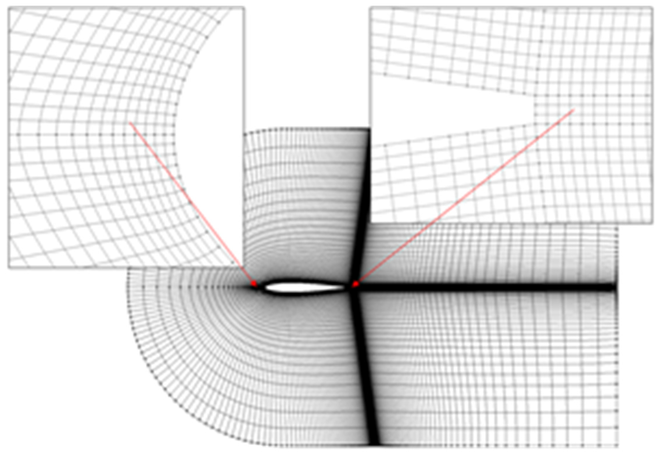
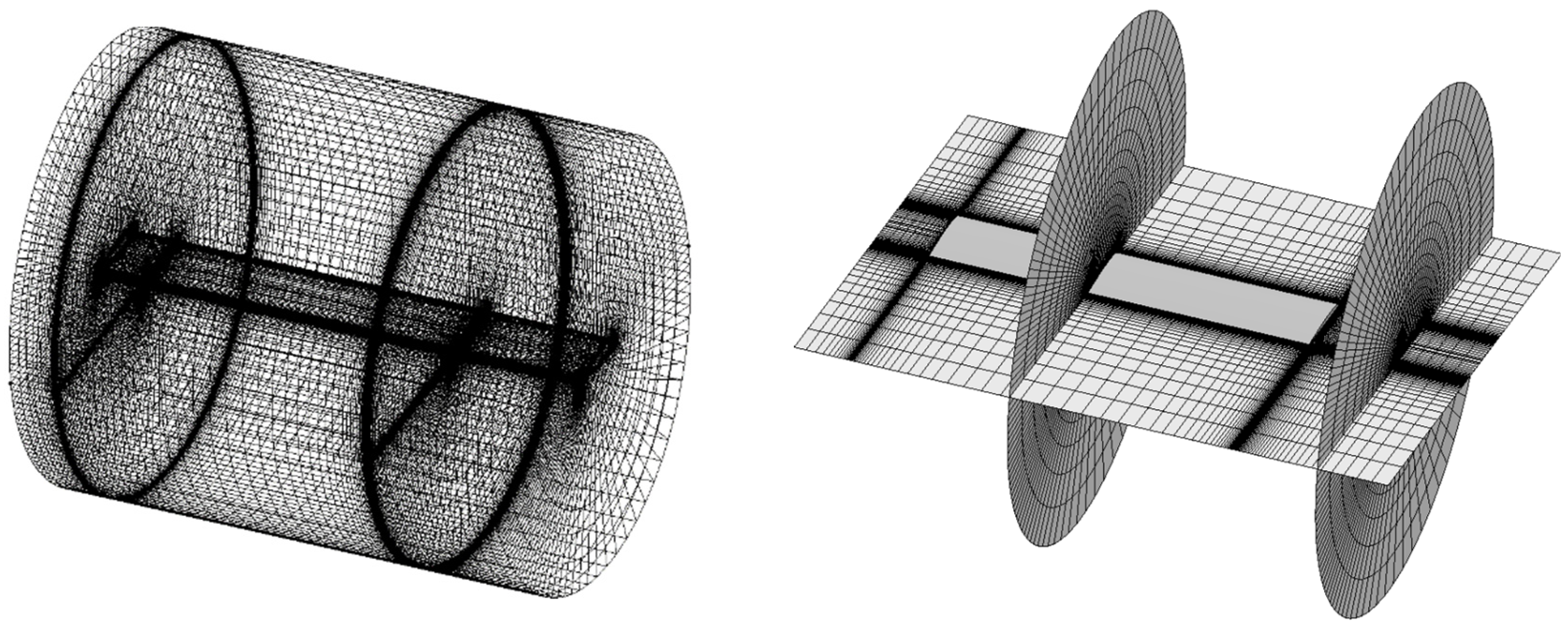
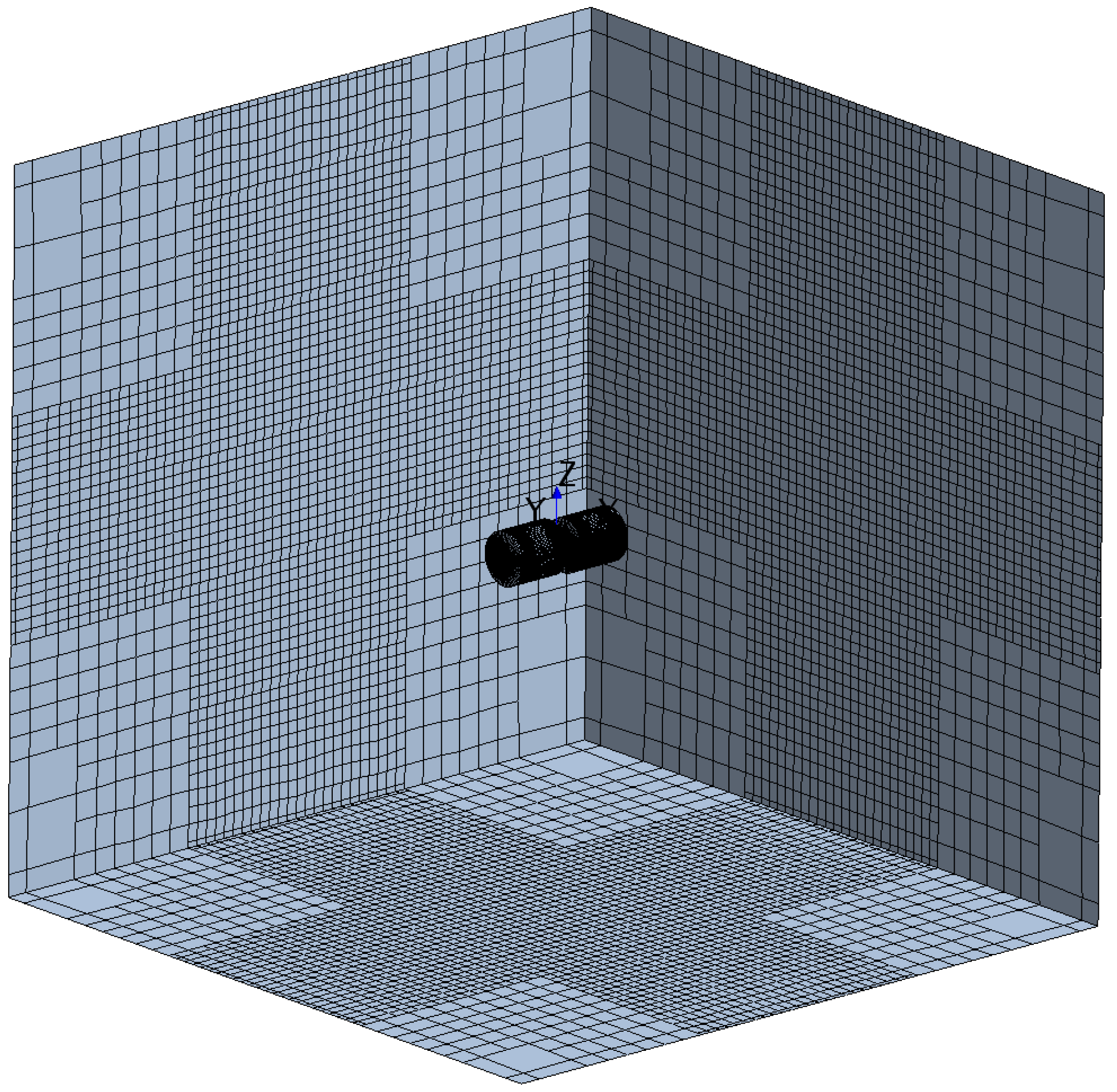
In this paper, each blade with uniform density is evenly distributed around the rotor shaft, so the center of mass of the whole rotor is located at the center of the rotor shaft, which is the origin of the rotor disk coordinate system. According to Newton’s law of motion, the six-degree of freedom equation of the rotor in space is expressed as follows:
m ( d V x d t + V z ω y V y ω z ) = F x m g sin θ m ( d V y d t + V x ω z V z ω x ) = F y m g cos θ cos γ m ( d V z d t + V y ω x V x ω y ) = F z m g cos θ sin γ I x d ω x d t + ( I z I y ) ω z ω y + I x y ( ω z ω x d ω y d t ) = M x I y d ω y d t + ( I x I z ) ω x ω z + I x y ( ω z ω y d ω x d t ) = M y I z d ω z d t + ( I y I x ) ω y ω x + I x y ( ω y 2 ω x 2 ) = M z
where m is the blade mass; θ is the pitch angle; γ is the roll angle; I x , I y , I z are the inertia moments; I x y is the inertia product; ω x , ω y ,   ω z are the three components of angular velocity; V x , V y , V z are the three components of water velocity; F x , F y , F z are the three components of the total aerodynamic force; and M x , M y , M z are the three components of the external moment. The convergence condition of the autorotation rotor is M z   = 0.

4. Grid System

In this paper, a structural overset grid system was developed, which can take into account the motion of the blade. The grid system is characterized by robustness and efficiency. The grid system consists of two kinds of grids: one is the blade body-fitted structural grid, and the second is the background structure grid, which belongs to the Cartesian grid and overlaps with the blade body-fitted grid to form a nested relationship.
The method of “plane to solid” was used to divide the blade’s grid. First, the blade was divided into grids on each blade element plane, and then the grids on blade element planes were combined to obtain a complete blade three-dimensional body-fitted grid. Finally, the algebraic method was used to generate the grids at the root and tip of the blade. Compared with the traditional elliptical grid generation method, the time required for mesh generation is reduced, although manual operations are increased. Furthermore, it can be extended to form high-quality meshes for blades with more complex shapes, which can demonstrate the tiny fluid flows on the blade surface.
As shown in Figure 5, the C-type mesh was selected as the blade body-fitted structure mesh. The two-dimensional cross section of the blade is distributed in an H-shape along the radial direction, resulting in a C-H blade body-fitted structure grid as shown in Figure 6. Due to the irregular shape of the blade tip, the flow field of autorotating rotors is inclined to have vortex dissipation. The advantage of using the H-shaped distribution is that the blade body-fitted structure grid has a high grid quality and is less capable of producing mesh distortion. In addition, this type of grid has high computational efficiency. In order to simulate blade tip vortex shedding, the mesh of the blade tip was encrypted in the radial direction.
There are two methods for the numerical CFD simulation of the rotor’s rotating flow field, a time multi-reference frame (MRF) model and a moving overset grid method.
In this paper, the moving overset grid method [57] was used to simulate the autorotating rotor. The flow field is divided into two parts: the motion region and the static region. The motion region is the blade grid. The 3D body-fitted grid of the blade is the moving grid. The static area is the background grid, as shown in Figure 7. In the process of grid nesting, it is necessary to dig holes and interpolate n the overlapping regions to ensure that the blade 3D body-fitted grid can be well-matched with the background grid near the blade.

5. Results and Discussion

In this section, the hydrodynamic characteristics of the underwater autorotating rotor are investigated. In the first three subsections of this section, the rotational speed, induced velocity, and tip vortex trajectory obtained from the test are compared with the CFD results to verify the accuracy of the CFD method. The fourth subsection calculates the thrust and thrust coefficients by the CFD method with different water velocities, shaft backward angles, blade pitches, blade twist angles, blade airfoils, and the number of blades.

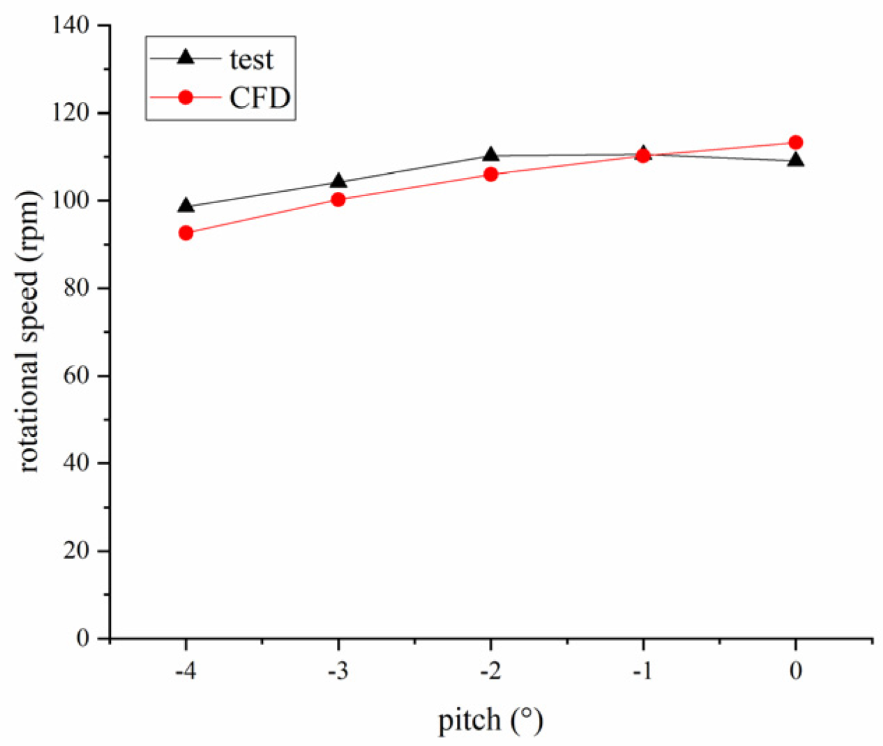
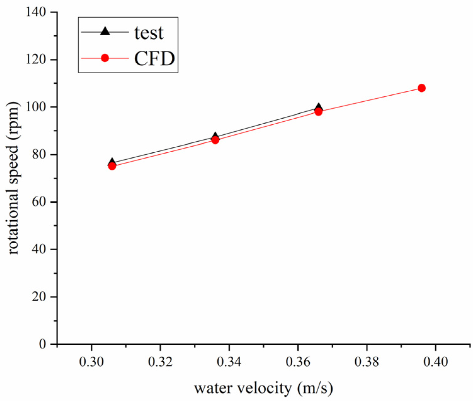
5.1. Rotational Speed

The pitch θ , water velocity v , and the shaft backward angle δ s were changed in the experiments to investigate the rotational speed of the underwater autorotating rotor.
The variation of rotational speed with δ s was shown in Figure 8. The rotational speed was linearly related to δ s .
The variation of rotational speed with θ is shown in Figure 9. A simple relationship between rotational speed and pitch is shown in Figure 8, first increasing and then decreasing, which was explained by the variable lift drag ratio with the angle of attack.
The variation of rotational speed with v is shown in Figure 10. There is an apparent positive linear correlation between rotational speed and water velocity.
It can be seen from Figure 8, Figure 9 and Figure 10 that the rotational speeds obtained by CFD simulation are generally in agreement with the test data. As can be seen from Table 2, the error is within 5%. As a result, the CFD simulations can be implemented for the calculation of the rotational speed.

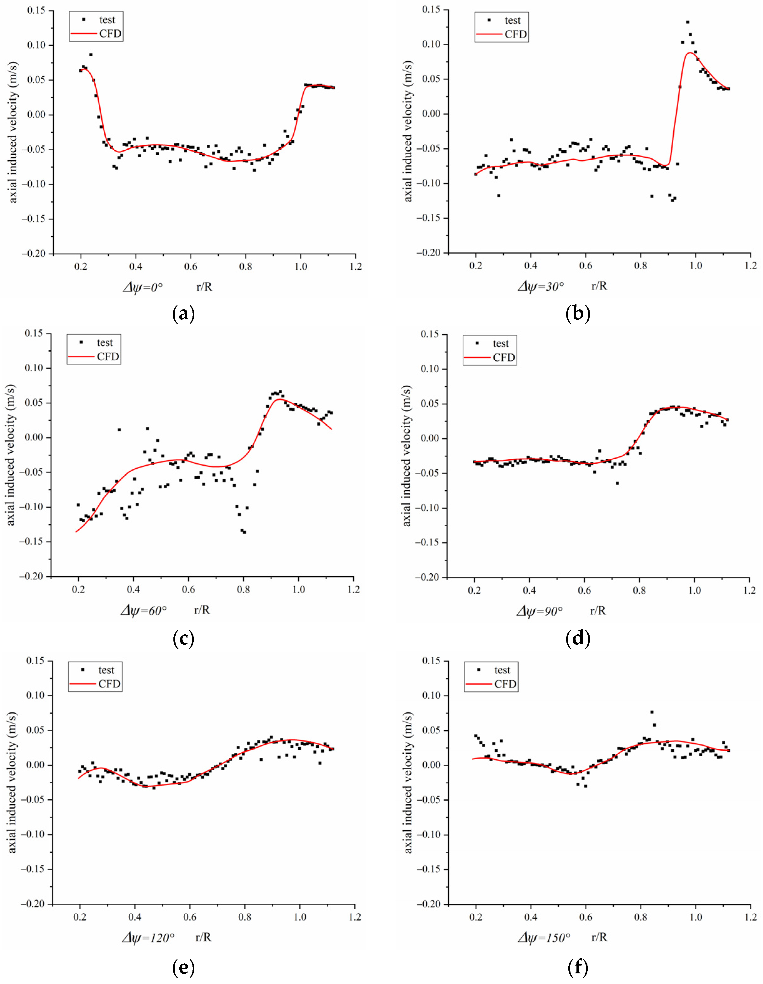
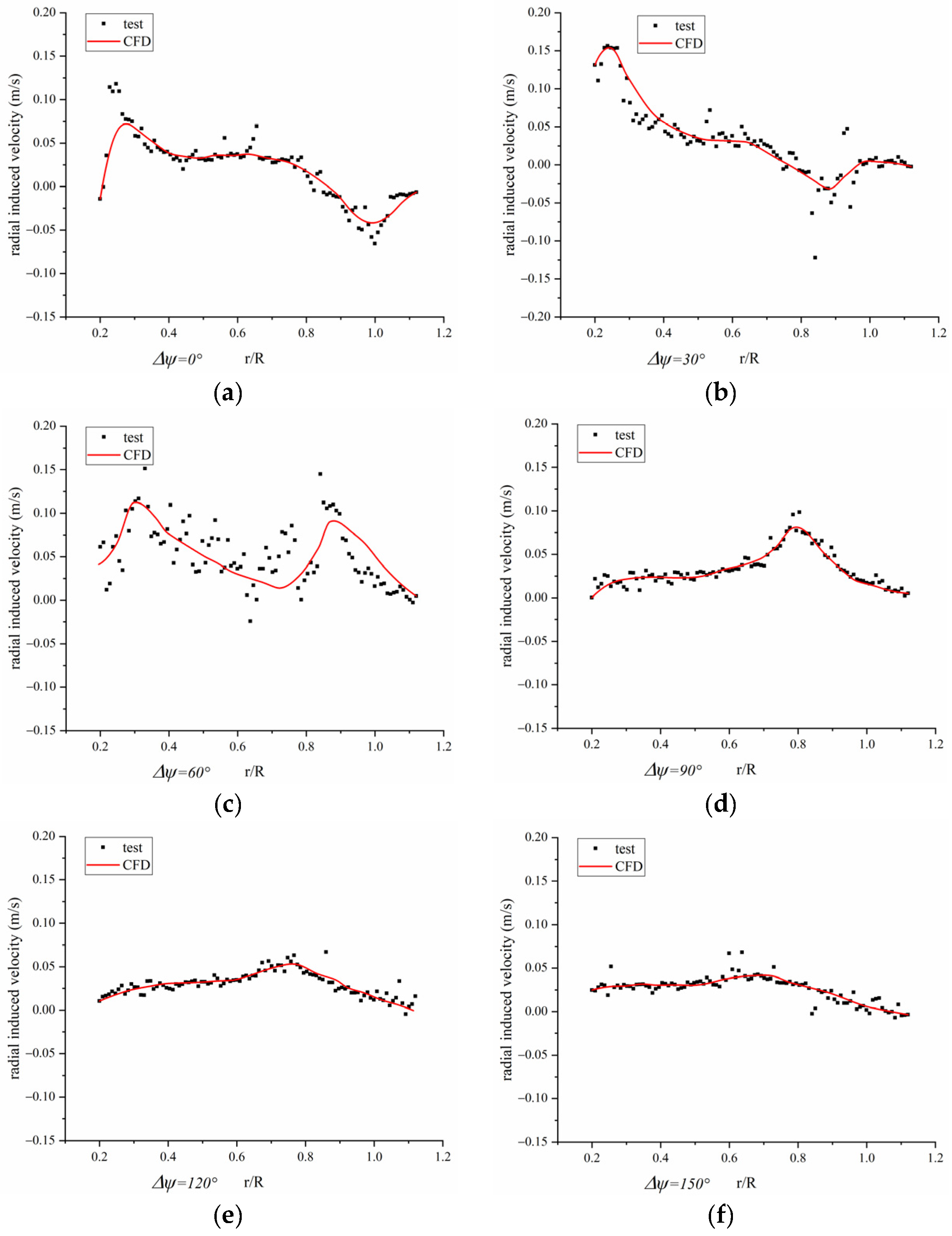
5.2. Induced Velocity

In this paper, when v = 0.306 m/s, δs = 40°, and θ = −3°, the induced velocity of the LW plane was investigated.
The LW plane recorded the longitudinal view of the axial-induced velocity viz and radial-induced velocity vir. Figure 11 shows the axial induced velocity at ψ = 180°. The positive axial induced speed is the decreasing z direction.
Figure 12 shows the radial induced velocity at ψ = 180°. The positive velocity direction is toward the blade tip. ∆ψ indicates the rotation angle of the blade after the blade position coincides with ψ = 180°.
As can be seen from Figure 11, the axial induced velocity is around 0.05 m/s. It is noteworthy that the induced velocity varies considerably at the blade root and tip, which was influenced by the hub, shaft, and tip vortices. This is a remarkable feature that the induced velocity after the blade tip drops rapidly to zero, which was influenced by tip vortices.
As shown in Figure 11 and Figure 12, the induced velocities obtained from CFD simulations correspond to the test data. Consequently, the CFD simulation method can be performed to calculate the induced velocity.
There are some reasons for the variation between CFD results and experimental results:
(1) The stable rotational speed calculated by CFD has some errors with the experimental results;
(2) The CFD calculation has not considered the interference of the hub and shaft;
(3) The experimental results have very few bad points.

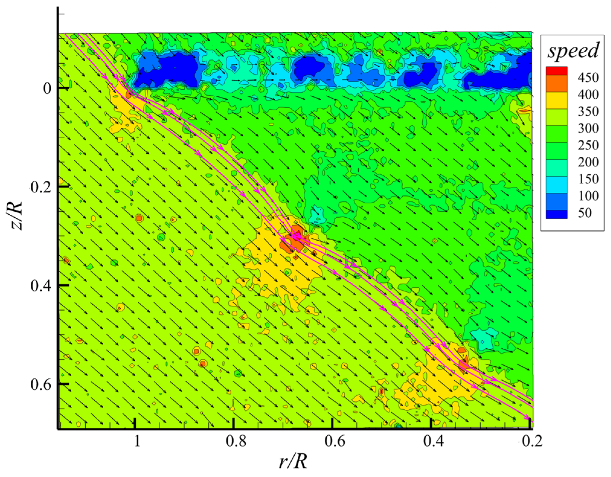
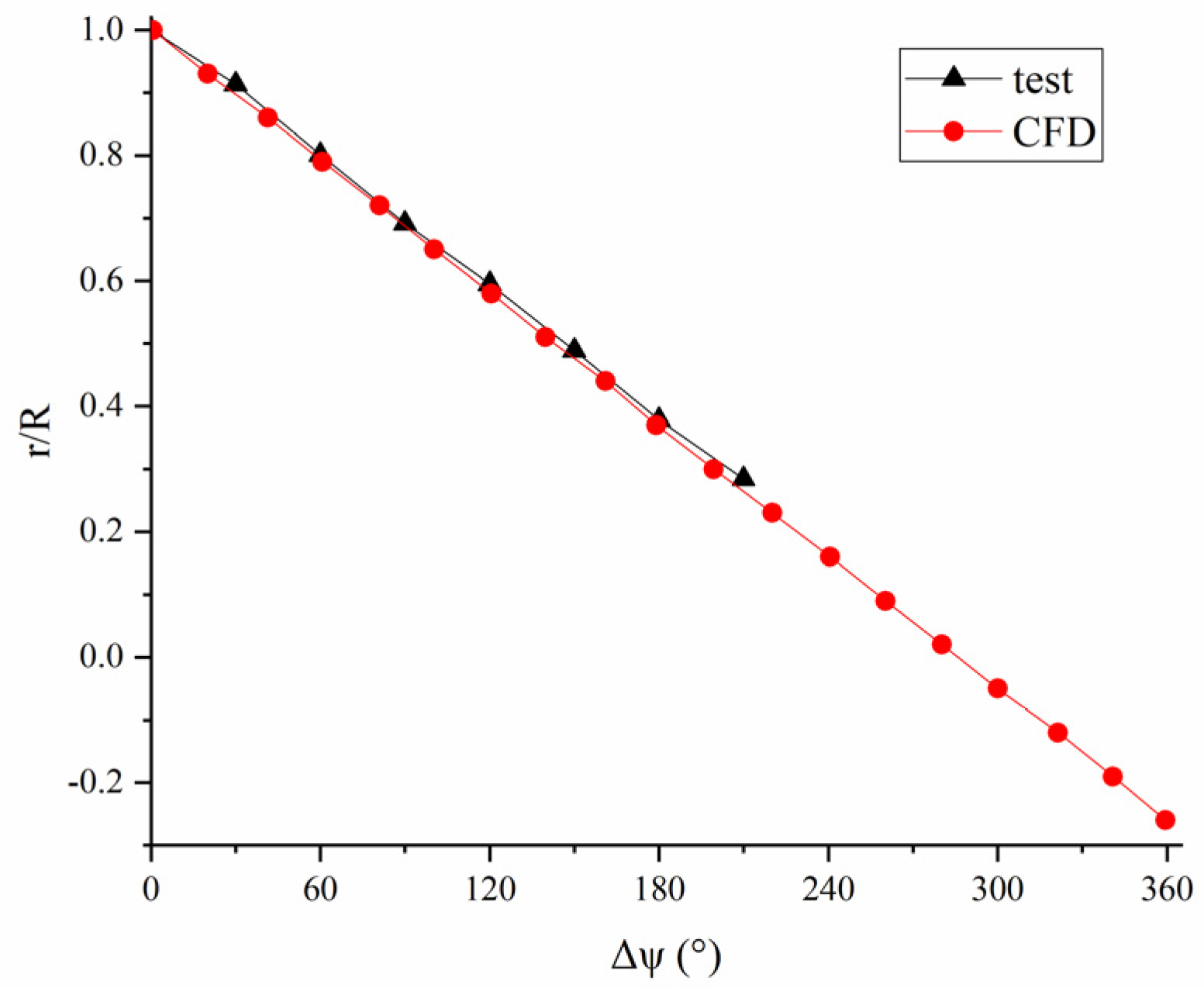
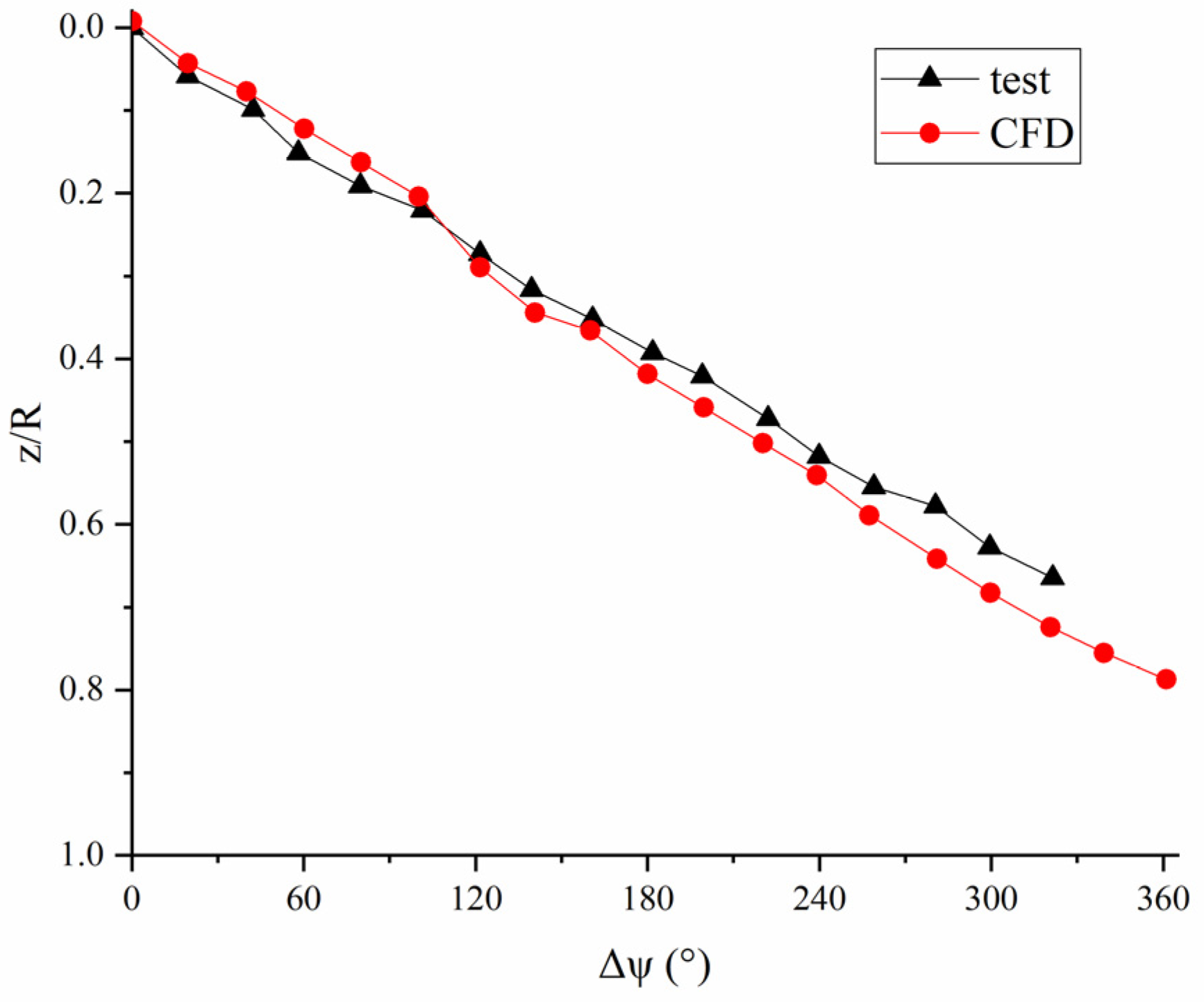
5.3. Tip Vortex Trajectory

In this paper, when v = 0.306 m/s, δs = 45°, and θ = −3°, the tip vortex trajectory was analyzed at ψ = 180°. The experimental results showed that the tip vortex trajectory at ψ = 0° was not significant, so it was not covered in this paper. Figure 13 illustrates the data provided by the experiments on tip vortex shedding trajectory at ψ = 180°.
Figure 14 and Figure 15 show the radial and axial displacements of the tip vortex, respectively. Both show a clear linear relationship with time. The results show a high degree of confidence that the CFD simulation data correspond to the test data. This demonstrates that the CFD simulations can be extended to the calculation of the tip vortex trajectory of the underwater autorotating rotor.

5.4. Thrust and Thrust Coefficient

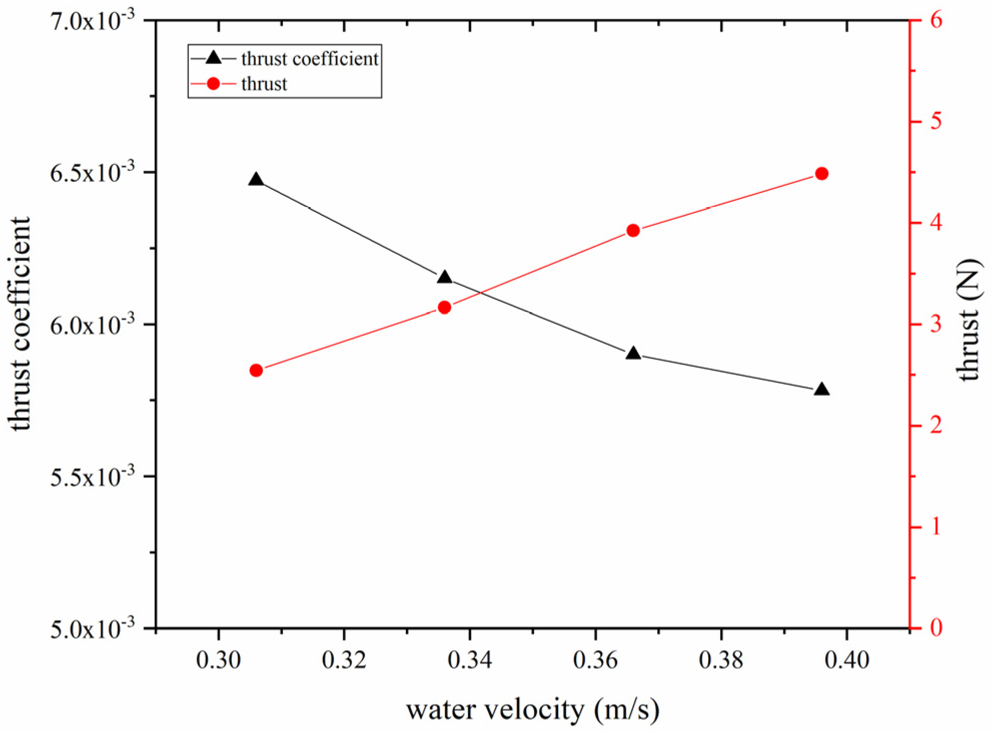
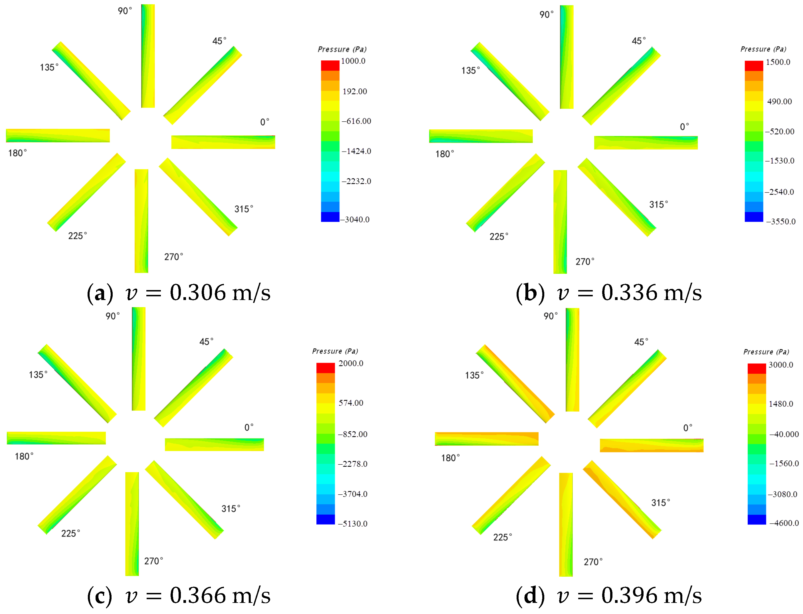
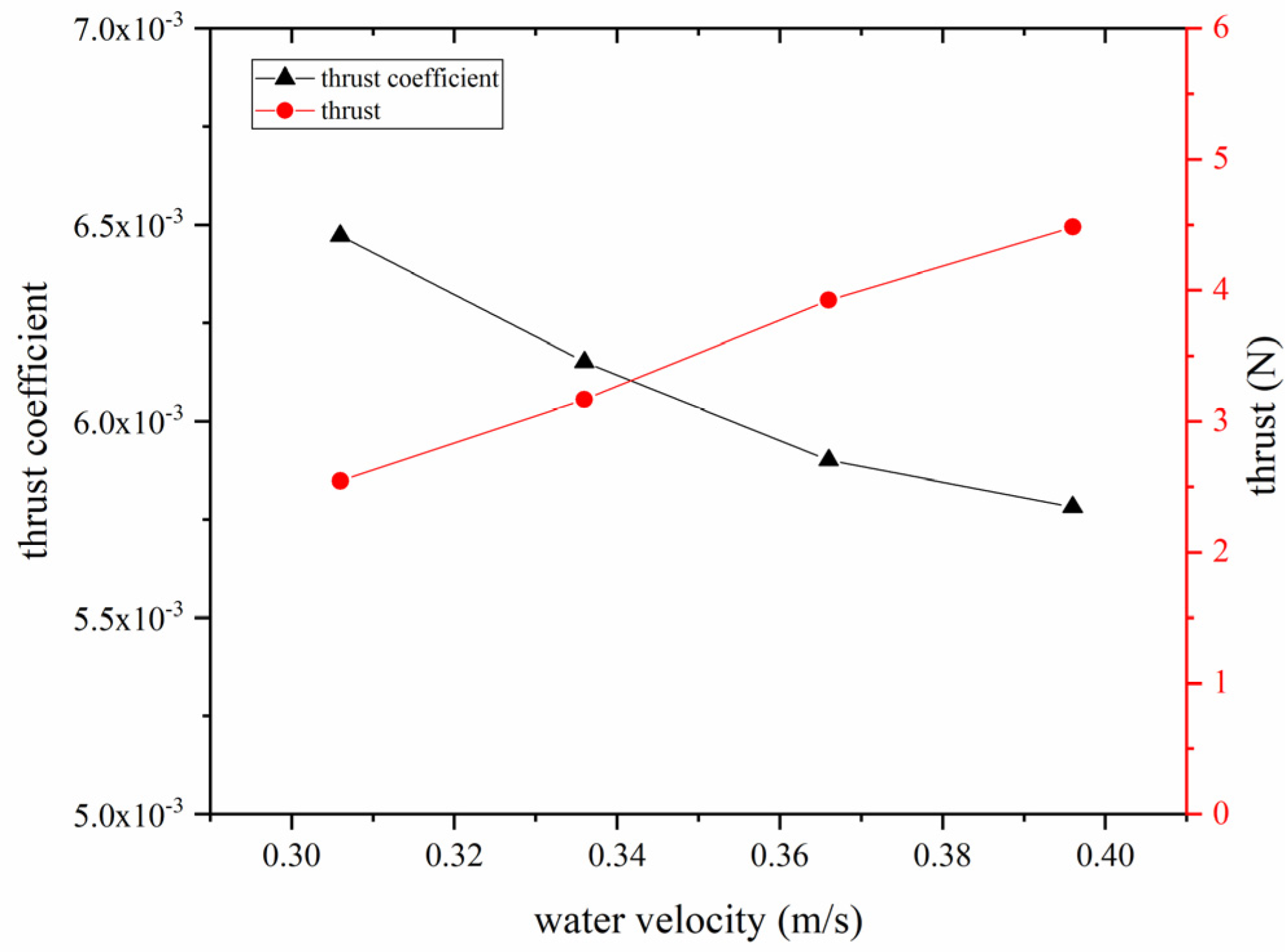
5.4.1. Water Velocity

When δs = 40°, and θ = −3°, the thrust T and the thrust coefficient CT was calculated by CFD simulation with water velocity v. As mentioned in the previous chapter, the rotational speed increases with the water velocity increase. Figure 16 shows the thrust and thrust coefficient with various water velocities. The thrust has a linear positive correlation with water velocity, while the thrust coefficient has a linear negative correlation with water velocity.
As the water speed increases, assuming that the rotational speed and induced velocity remain constant, the angle of attack of the blade will increase in order to achieve zero torque equilibrium conditions, which results in the lift component in the rotor disc exceeding the drag component. Thus, this results in an increase in the rotor driving region, which leads to increasing rotational speed and thrust.
The pressure distribution on the blade upper surface at various water velocities is illustrated in Figure 17. As the water velocity increases, the negative pressure area on the blade’s upper surface expands, while the positive pressure at the blade’s leading edge also appears to increase. The maximum and minimum negative pressure peaks on the blade’s upper surface occur at ψ = 135° and 315°, respectively. The smaller the peak negative pressure on the blade’s upper surface, the more favorable it is to delay the occurrence of air separation. As a result, when the water velocity exceeds a critical value, airflow separation will occur on the blade’s upper surface, and thus a stall zone will appear at the blade tip, and the thrust coefficient will drop rapidly.

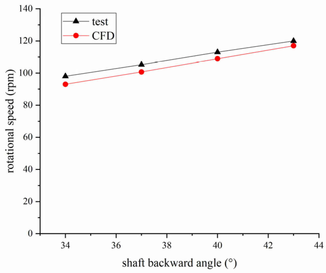
5.4.2. Shaft Backward Angle
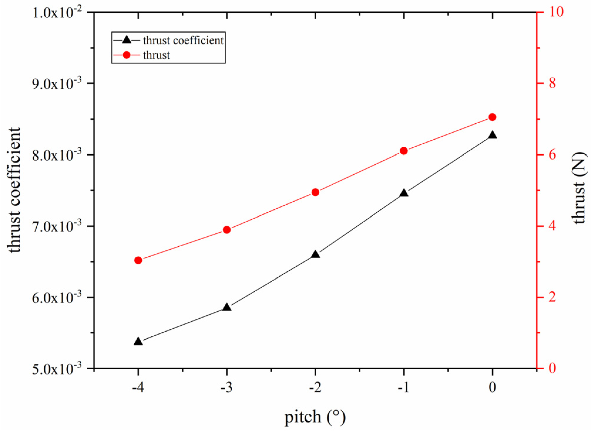
When v = 0.366 m/s and θ = 0°, the thrust T and thrust coefficient CT was calculated by CFD simulation with the shaft backward angle δs. Figure 18 show the thrust and thrust coefficient with various shaft backward angles. As can be clearly seen in Figure 18 the thrust force is linearly and positively related to the shaft backward angle. However, the thrust coefficient scarcely varies with the shaft backward angle.
Figure 19 shows the force analysis of the blade profile. The increase in the shaft backward angle causes the vertical velocity Up to rise. The tangential component of water velocity in the rotor disc is negligible relative to the blade’s rotational linear velocity, so that UT is essentially close to the blade’s rotational linear velocity. Thus, at a fixed rotational speed, the angle of attack α increases as the shaft backward angle increases, resulting in an increase in the lift dL and drag dD. The increase in angle of attack α also leads to an increase in the lift-to-drag ratio, so that the increment of the lift component dL is greater than the increment of the drag component dD in the horizontal direction, which in turn generates a driving force that increases the rotor speed. An increase in rotor speed leads to a decrease in the angle of attack α. So, the increase in the vertical component of the total force dR causes an increase in the thrust. According to CFD simulation data, the rotational speed increases as the shaft backward angle increases, but the ratio Up/ΩR remains essentially unchanged. This indicates that the angle of attack α remains essentially the same and so the thrust coefficient does not respond essentially to variation in the shaft backward angle.

5.4.3. Blade Pitch

When v = 0.366 m/s and δs = 40°, the thrust T and thrust coefficient CT was calculated by CFD simulation with θ. Figure 20 shows the thrust and thrust coefficient with various pitches. From Figure 20, we can see clearly that the thrust and thrust coefficient have a linear positive correlation with the pitch.
With the increase in the pitch, the inflow angle ϕ increases, which leads to the increase in the vertical component of the resultant force dR and the increase in the thrust. Because the ratio of Up/ΩR increases, the angle of attack α of increases leading to an increase in the thrust coefficient.
As the pitch increases, the inflow angle ϕ increases, which leads to an increase in the vertical component of the resultant force dR. Ultimately, the thrust force increases. As the ratio Up/ΩR increases, an increase in the angle of attack α induces an increase in the thrust coefficient.

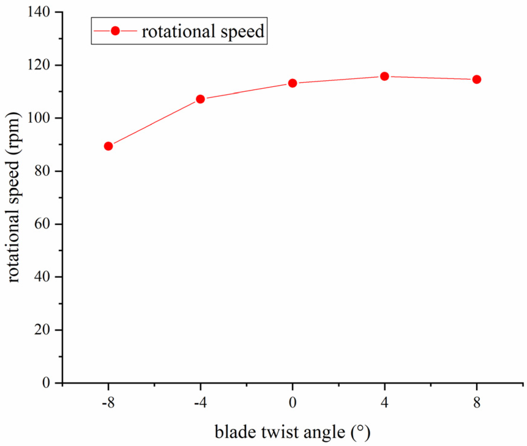
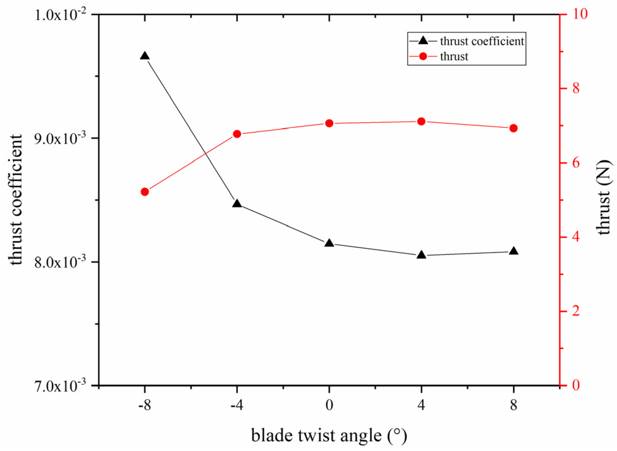
5.4.4. Blade Twist Angle

The blade torsion angle is one of the most important geometrical features of a rotor and it has an influential effect on the hydrodynamic characteristics of underwater autorotating rotors. In this paper, the hydrodynamic characteristics with blade torsion angles of −8°, −4°, 0°, 4°, and 8° are investigated.
The variation of rotational speed with blade twist angles is shown in Figure 21. Within a certain range, the rotational speed under negative torsion is less than that without torsion.
When v = 0.366 m/s, θ = 0°, and δs = 40°, the thrust T and thrust coefficient CT was calculated by CFD simulation with the blade twist angle. Figure 22 shows the thrust and thrust coefficient with various blade twist angle. The thrust has a positive correlation with the blade twist angle, while the thrust coefficient has a negative correlation with the blade twist angle.
Within a certain range, the angle of attack at the blade root decreases due to positive torsion, reducing the stall region. The blade tip lift-to-drag ratio increases, the driving region expands outward and the driven region decreases, thus increasing the rotational speed. However, when the speed exceeds a specific value, the blade tip stalls, resulting in a reduction in rotational speed. Due to the fact that the driving region makes up the majority of the rotor disc, the angle of attack in this region decreases as the blade torsion angle increases, so the thrust coefficient decreases gradually. However, excessive positive twisting of the blade can lead to a decrease in thrust and an increase in thrust coefficient.

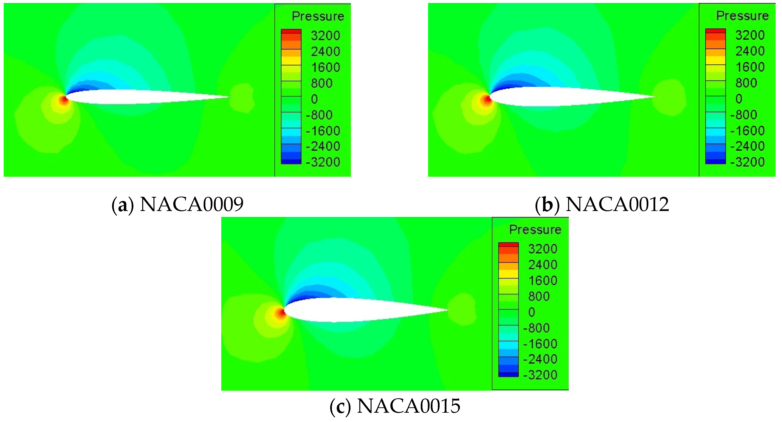
5.4.5. Blade Airfoil

When v = 0.366 m/s, θ = 0°, and δs = 40°, the thrust T and thrust coefficient CT with different blade airfoils was calculated by CFD simulation with various blade airfoils. Table 3 shows the thrust and thrust coefficient with various blade airfoils.
This paper investigates the effect of a symmetrical airfoil on the hydrodynamic characteristics of underwater autorotating rotors. As the relative thickness of the blade airfoil increases, the speed and thrust decrease but the thrust coefficient increases. This is because, as the relative thickness of the blade airfoil increases, the lift-to-drag ratio decreases at low Reynolds numbers. This situation causes the zero-torque position of the rotor disc to move outward, resulting in an enlarged area of the driving region and an enhanced rotational speed.
The pressure distribution on the upper surface of the advancing blade at 0.9R is shown in Figure 23. The area of negative pressure distribution on both the upper and lower surfaces of the blade increases with increasing blade relative thickness, but the negative pressure on the lower surface increases more noticeably. At the trailing edge of the blade, the greatest positive pressure is found on the NACA0012 airfoil.

5.4.6. Number of Blades

When v = 0.366 m/s, θ = 0°, and δs = 40°, the thrust T and thrust coefficient CT was calculated by CFD simulation with various numbers of blades. Table 4 shows the thrust and thrust coefficient with various numbers of blades.
We can see from Table 4 that an increase in the number of blades results in a decrease in rotational speed but an increase in thrust and thrust coefficient. However, the aerodynamic interference between the blades increases with the number of blades. When the interference between blade aerodynamics is too large, the increase in the number of blades fails to enlarge the thrust and thrust coefficient.
The autorotation of an underwater rotor is the conversion of kinetic energy between the water and the rotor. In this process, the loss of kinetic energy of the water is limited. Therefore, as the number of blades increases, the amount of energy gained by each blade decreases, causing a reduction in the rotational speed. The increase in the number of blades means that the rotor solidity increases, which makes the thrust coefficient increase. The kinetic energy of the water will not be able to drive the rotor rotation when the rotor solidity reaches a critical value.

6. Conclusions

In this paper, PIV tests and CFD simulations were carried out to investigate the hydrodynamic characteristics of underwater autorotating rotors. The underwater autorotating rotor was tested and investigated in terms of three aspects: rotational speed, induced velocity, and tip vortex trajectory, and the test results were used to validate the accuracy of the CFD simulations. The CFD simulations were used to calculate the thrust and thrust coefficient of the underwater autorotating rotor in terms of six aspects: water velocity, shaft back angle, pitch, twist angle, and blade numbers. The following conclusions were drawn from this work.
  • The experimental results show that the rotational speed has a significant positive correlation with the water velocity and shaft backward angle, but the relationship with the pitch is first increasing and then decreasing. The axial-induced velocity is around 0.05 m/s. The induced velocity fluctuates sharply around the blade tip and rapidly drops to zero outside the blade tip. The dramatic variations are due to the effect of the water velocity and the blade tip vortices. The radial and axial displacements of blade tip vortex trajectories are clearly linear with respect to time.
  • A computational fluid dynamic (CFD) based on moving overset grids was developed to study the hydrodynamic characteristics of the underwater autorotating rotor. In this simulation, the Navier–Stokes equations were solved using the overset grids technique to calculate the flow field of the underwater autorotating rotor under various states. The experimental results demonstrate that CFD simulation method is suitable for investigating the hydrodynamic characteristics of underwater autorotating rotors. Induced velocity verifies the accuracy of the simulated velocity flow field. The position of the blade tip vortex trajectory confirms the accuracy of the simulated blade tip complex flow field.
  • The thrust has a linear positive correlation with water velocity, but the thrust coefficient has a linear negative correlation with water velocity. When the water speed exceeds a certain value, waterflow separation occurs on the blade upper surface resulting in the emergence of a stall region at blade tip, which causes the thrust coefficient to drop rapidly.
  • The thrust is linearly related to the shaft backward angle, but the thrust coefficient is almost a fixed value with δs. However, an excessively large shaft backward angle increases drag in the forward direction, so it is essential to select a properly angled shaft back. The thrust and thrust coefficient are linearly and positively correlated with the blade pitch as the blade pitch increases from a negative value to zero.
  • As the blade twist angle changes from negative to positive, the thrust first increases and then tends to stable, in contrast to the decrease in the thrust coefficient. Therefore, a suitable negative blade torsion is more advantageous for underwater autorotating rotors. However, the excessive positive twist of the blade can lead to a decrease in thrust and an increase in thrust coefficient. For symmetrical airfoils, within a certain range, as the airfoil thickness increases, the rotational speed, and thrust decrease, but the thrust coefficient increases. Appropriately thin airfoils are more beneficial for underwater autorotating rotors. An increase in the number of blades increases thrust and thrust coefficient but reduces rotational speed. The rotor will not rotate when the number of blades reaches a specific value. When the rotor can be rotated, the number of blades can be increased appropriately to improve the performance of underwater autorotating rotors.
  • All our preliminary results throw light on the fundamental characteristics of underwater autorotating rotors. A limitation of this study is that the blade deformation is not considered in the CFD simulations. Further research should be carried out on multiple blades to enrich the theory of underwater autorotating rotors.

Author Contributions

Conceptualization, L.L.; methodology, L.L.; software, L.L. and Z.W.; validation, L.L.; formal analysis, Z.W.; investigation, A.X. and F.W.; resources, M.C. and F.W.; data curation, L.L.; writing—original draft preparation, L.L. and Z.W.; writing—review and editing, L.L.; visualization, M.C. and F.W.; supervision, M.C.; project administration, A.X.; funding acquisition, F.W. and M.C. All authors have read and agreed to the published version of the manuscript.

Funding

This study was funded by the National Key Research and Development Project of China (No. 2021YFC3002105).

Institutional Review Board Statement

Not applicable.

Informed Consent Statement

Not applicable.

Data Availability Statement

The data presented in this study are available on request from the corresponding author.

Acknowledgments

The authors are grateful to the Unmanned Helicopter Research Institute of Beihang University for assistance during the designing of the experiments.

Conflicts of Interest

The authors declare no conflict of interest.

References

  1. Song, L.; Zhang, H.; Liu, Y.; Wang, Y.; Yang, Y. Research on negative-buoyancy autorotating-rotor autonomous underwater vehicles. Appl. Ocean Res. 2020, 99, 102123. [Google Scholar] [CrossRef]
  2. Panda, J.P.; Mitra, A.; Warrior, H.V. A review on the hydrodynamic characteristics of autonomous underwater vehicles. Proc. Inst. Mech. Eng. Part M J. Eng. Marit. Environ. 2021, 235, 15–29. [Google Scholar] [CrossRef]
  3. Wang, Z.K.; Liu, X.; Huang, H.C.; Chen, Y. Development of an autonomous underwater helicopter with high maneuverability. Appl. Sci. 2019, 9, 4072. [Google Scholar] [CrossRef] [Green Version]
  4. Petritoli, E.; Leccese, F. Unmanned autogyro for mars exploration: A preliminary study. Drones 2021, 5, 53. [Google Scholar] [CrossRef]
  5. Sharma, M.; Gupta, A.; Gupta, S.K.; Alsamhi, S.H.; Shvetsov, A.V. Survey on unmanned aerial vehicle for mars exploration: Deployment use case. Drones 2022, 6, 4. [Google Scholar] [CrossRef]
  6. De la Cierva, J. New developments of the autogiro. Aeronaut. J. 1935, 39, 1125–1143. [Google Scholar] [CrossRef]
  7. Tokaty, G.A. A History and Philosophy of Fluid Mechanics; Courier Corporation: Chelmsford, MA, USA, 1994. [Google Scholar]
  8. Leishman, J.G. Principles of Helicopter Aerodynamics, 2nd ed.; Cambridge University Press: New York, NY, USA, 2006. [Google Scholar]
  9. Leishman, J.G. Development of the autogiro: A technical perspective. J. Aircr. 2004, 41, 765–781. [Google Scholar] [CrossRef]
  10. Glauert, H. A General Theory of the Autogyro; HM Stationery Office: Richmond, UK, 1926. [Google Scholar]
  11. Wheatley, J.B. Lift and Drag Characteristics and Gliding Performance of an Autogiro as Determined in Flight; NACA-TR-434; National Advisory Committee for Aeronautics: Washington, DC, USA, 1933.
  12. Wheatley, J.B. The Aerodynamic Analysis of the Gyroplane Rotating-Wing System; NACA-TN-492; National Advisory Committee for Aeronautics: Washington, DC, USA, 1934.
  13. Wheatley, J.B. A Study of Autogiro Rotor-Blade Oscillations in the Plane of the Rotor Disk; NACA-TN-581; National Advisory Committee for Aeronautics: Washington, DC, USA, 1936.
  14. Wheatley, J.B. An Analysis of the Factors that Determine the Periodic Twist of an Autogiro Rotor Blade, with a Comparison of Predicted and Measured Results; NACA-TR-600; National Advisory Committee for Aeronautics: Washington, DC, USA, 1937.
  15. Wheatley, J.B. An Analytical and Experimental Study of the Effect of Periodic Blade Twist on the Thrust, Torque, and Flapping Motion of an Autogiro Rotor; NACA-TR-591; US Government Printing Office: Washington, DC, USA, 1937.
  16. Wheatley, J.B.; Bioletti, C. Analysis and Model Tests of Autogiro Jump Take-Off; NACA-TN-582; National Advisory Committee for Aeronautics: Washington, DC, USA, 1936.
  17. Wheatley, J.B.; Bioletti, C. Wind-tunnel, tests of 10-foot-diameter auto giro rotors. In Annual Report-National Advisory Committee for Aeronautics; United States Government Publishing Office: Washington, DC, USA, 1937; p. 199. [Google Scholar]
  18. Houston, S. Identification of autogyro longitudinal stability and control characteristics. J. Guid. Control Dyn. 1998, 21, 391–399. [Google Scholar] [CrossRef]
  19. Houston, S. Validation of a rotorcraft mathematical model for autogyro simulation. J. Aircr. 2000, 37, 403–409. [Google Scholar] [CrossRef]
  20. Houston, S. Analysis of rotorcraft flight dynamics in autorotation. J. Aircr. 2002, 25, 33–39. [Google Scholar] [CrossRef]
  21. Houston, S. Modeling and analysis of helicopter flight mechanics in autorotation. J. Aircr. 2003, 40, 675–682. [Google Scholar] [CrossRef]
  22. Houston, S.; Brown, R. Rotor-wake modeling for simulation of helicopter flight mechanics in autorotation. J. Aircr. 2003, 40, 938–945. [Google Scholar] [CrossRef]
  23. Thomson, D.; Houston, S. Application of parameter estimation to improved autogyro simulation model fidelity. J. Aircr. 2005, 42, 33–40. [Google Scholar] [CrossRef]
  24. Bagiev, M.; Thomson, D.G.; Houston, S. Autogyro handling qualities assessment. In Proceedings of the 60th American Helicopter Society Annual Forum, Baltimore, MD, USA, 7–10 June 2004. [Google Scholar]
  25. Bagiev, M.; Thomson, D.G. Handling qualities evaluation of an autogiro against the existing rotorcraft criteria. J. Aircr. 2009, 46, 168–174. [Google Scholar] [CrossRef]
  26. Bagiev, M.; Thomson, D.G. Handling qualities assessment of an autogiro. J. Am. Helicopter Soc. 2010, 55, 32003. [Google Scholar] [CrossRef]
  27. Eriksen, C.C.; Osse, T.J.; Light, R.D.; Wen, T.; Lehman, T.W.; Sabin, P.L.; Ballard, J.W.; Chiodi, A.M. Seaglider: A long-range autonomous underwater vehicle for oceanographic research. IEEE J. Ocean. Eng. 2001, 26, 424–436. [Google Scholar] [CrossRef] [Green Version]
  28. Webb, D.C.; Simonetti, P.J.; Jones, C.P. SLOCUM: An underwater glider propelled by environmental energy. IEEE J. Ocean. Eng. 2001, 26, 447–452. [Google Scholar] [CrossRef]
  29. Li, X.; Zhao, M.; Zhao, F.; Yuan, Q.; Ge, T. Study on hydrodynamic performance of heavier-than-water AUV with overlapping grid method. Ocean Syst. Eng. 2014, 4, 1–19. [Google Scholar] [CrossRef] [Green Version]
  30. Herrero, A.D.; Percin, M.; Karasek, M.; van Oudheusden, B. Flow visualization around a flapping-wing micro air vehicle in free flight using large-scale PIV. Aerospace 2018, 5, 99. [Google Scholar] [CrossRef] [Green Version]
  31. Yin, K.W.; Zhang, J.; Chen, S. Design of a high uniformity laser sheet optical system for particle image velocimetry. Aerospace 2021, 8, 393. [Google Scholar] [CrossRef]
  32. Deng, Y.-M. PIV measurement of water tunnel for the flow field of a hovering coaxial-rotor. J. Aerosp. Power 2007, 22, 1852–1857. [Google Scholar]
  33. Yu, S.; Deng, Y. PIV measurements in the wake of coaxial-rotor in water tunnel. J. Beijing Univ. Aeronaut. Astronaut. 2007, 33, 635–639. [Google Scholar]
  34. Zanotti, A. Experimental study of the aerodynamic interaction between side-by-side propellers in evtol airplane mode through stereoscopic particle image velocimetry. Aerospace 2021, 8, 239. [Google Scholar] [CrossRef]
  35. De Gregorio, F.; Pengel, K.; Kindler, K. A comprehensive PIV measurement campaign on a fully equipped helicopter model. Exp. Fluids 2012, 53, 37–49. [Google Scholar] [CrossRef]
  36. Ma, Y.; Chen, M.; Zhang, X.; Wang, Q. Scale-model tests of coaxial rotors in water tunnel via particle image velocimetry technique. Proc. Inst. Mech. Eng. Part G J. Aerosp. Eng. 2016, 230, 426–443. [Google Scholar] [CrossRef]
  37. Mortimer, P.; Sirohi, J.; Platzer, S.; Rauleder, J. Coaxial rotor wake measurements in hover using phase-resolved and time-resolved PIV. In Proceedings of the Vertical Flight Society 75th Annual Forum, Philadelphia, PA, USA, 13–16 May 2019. [Google Scholar]
  38. Costes, M.; Renaud, T.; Rodriguez, B. Rotorcraft simulations: A challenge for CFD. Int. J. Comput. Fluid Dyn. 2012, 26, 383–405. [Google Scholar] [CrossRef]
  39. Sugiura, M.; Tanabe, Y.; Sugawara, H. Development of a hybrid method of CFD and prescribed wake model for helicopter BVI noise prediction. Trans. Jpn. Soc. Aeronaut. Space Sci. 2013, 56, 343–350. [Google Scholar] [CrossRef] [Green Version]
  40. Batrakov, A.; Kusyumov, A.; Kusyumov, S.; Mikhailov, S.; Barakos, G.N. Simulation of tail boom vibrations using main rotor-fuselage computational fluid dynamics (CFD). Appl. Sci. 2017, 7, 918. [Google Scholar] [CrossRef] [Green Version]
  41. Strawn, R.C.; Duque, E.P.N.; Ahmad, J. Rotorcraft aeroacoustics computations with overset-grid CFD methods. J. Am. Helicopter Soc. 1999, 44, 132–140. [Google Scholar] [CrossRef]
  42. Pomin, H.; Wagner, S. Navier-Stokes analysis of helicopter rotor aerodynamics in hover and forward flight. J. Aircr. 2002, 39, 813–821. [Google Scholar] [CrossRef]
  43. Potsdam, M.; Yeo, H.; Johnson, W. Rotor airloads prediction using loose aerodynamic/structural coupling. J. Aircr. 2006, 43, 732–742. [Google Scholar] [CrossRef]
  44. Nielsen, E.J.; Diskin, B. Discrete adjoint-based design for unsteady turbulent flows on dynamic overset unstructured grids. AIAA J. 2013, 51, 1355–1373. [Google Scholar] [CrossRef]
  45. Jarkowski, M.; Woodgate, M.A.; Barakos, G.N.; Rokicki, J. Towards consistent hybrid overset mesh methods for rotorcraft CFD. Int. J. Numer. Methods Fluids 2014, 74, 543–576. [Google Scholar] [CrossRef]
  46. Vassberg, J.C.; Tinoco, E.N.; Mani, M.; Rider, B.; Zickuhr, T.; Levy, D.W.; Brodersen, O.P.; Eisfeld, B.; Crippa, S.; Wahls, R.A.; et al. Summary of the fourth AIAA computational fluid dynamics drag prediction workshop. J. Aircr. 2014, 51, 1070–1089. [Google Scholar] [CrossRef]
  47. Ishikawa, H.; Koganezawa, S.; Makino, Y. Unstructured/structured overset grid simulation for the third AIAA sonic boom prediction workshop. J. Aircr. 2022, 59, 660–669. [Google Scholar] [CrossRef]
  48. Yang, Y.C.; Xu, G.H.; Shi, Y.J. Research on a robust overset grid method for load calculation of coaxial rotor. Int. J. Aeronaut. Space Sci. 2022, 23, 484–500. [Google Scholar] [CrossRef]
  49. Lu, L.; Yan, X.P.; Li, Q.; Wang, C.; Shen, K.C. Numerical study on the water-entry of asynchronous parallel projectiles at a high vertical entry speed. Ocean Eng. 2022, 250, 111026. [Google Scholar] [CrossRef]
  50. Kim, H.; Ranmuthugala, D.; Leong, Z.Q.; Chin, C. Six-DOF simulations of an underwater vehicle undergoing straight line and steady turning manoeuvres. Ocean Eng. 2018, 150, 102–112. [Google Scholar] [CrossRef]
  51. Drews, P.L.J.; Neto, A.A.; Campos, M.F.M. Hybrid Unmanned Aerial Underwater Vehicle: Modeling and Simulation. In Proceedings of the IEEE/RSJ International Conference on Intelligent Robots and Systems (IROS), Chicago, IL, USA, 14–18 September 2014; pp. 4637–4642. [Google Scholar]
  52. Kilavuz, A.; Ozgoren, M.; Kavurmacioglu, L.A.; Durhasan, T.; Sarigiguzel, F.; Sahin, B.; Akilli, H.; Sekeroglu, E.; Yaniktepe, B. Flow characteristics comparison of PIV and numerical prediction results for an unmanned underwater vehicle positioned close to the free surface. Appl. Ocean Res. 2022, 129, 103399. [Google Scholar] [CrossRef]
  53. Gao, T.; Wang, Y.; Pang, Y.; Cao, J. Hull shape optimization for autonomous underwater vehicles using CFD. Eng. Appl. Comput. Fluid Mech. 2016, 10, 599–607. [Google Scholar] [CrossRef] [Green Version]
  54. Hong, L.; Fang, R.J.; Cai, X.T.; Wang, X. Numerical Investigation on Hydrodynamic Performance of a Portable AUV. J. Mar. Sci. Eng. 2021, 9, 812. [Google Scholar] [CrossRef]
  55. Baaijens, F.P. Mixed finite element methods for viscoelastic flow analysis: A review. J. Non-Newton. Fluid Mech. 1998, 79, 361–385. [Google Scholar] [CrossRef]
  56. Baldwin, B.; Lomax, H. Thin-layer approximation and algebraic model for separated turbulentflows. In Proceedings of the 16th Aerospace Sciences Meeting, Huntsville, AL, USA, 16–18 January 1978; p. 257. [Google Scholar]
  57. Takahashi, S.; Monjugawa, I.; Nakahashi, K. Unsteady flow computations around moving airfoils by overset unstructured grid method. Trans. Jpn. Soc. Aeronaut. Space Sci. 2008, 51, 78–85. [Google Scholar] [CrossRef]
Figure 1. Configuration of water tunnel.
Aerospace 10 00020 g001
Figure 2. The experiment set-up.
Aerospace 10 00020 g002
Figure 3. Longitudinal window set-up.
Aerospace 10 00020 g003
Figure 4. Flow diagram of the dual time stepping method for overset grid.
Aerospace 10 00020 g004
Figure 5. The C type mesh.
Aerospace 10 00020 g005
Figure 6. Three-dimensional blade body-fitted grid.
Aerospace 10 00020 g006
Figure 7. The background grids.
Aerospace 10 00020 g007
Figure 8. Rotational speed with δ s at θ = 0°, v = 0.306 m/s.
Aerospace 10 00020 g008
Figure 9. Rotational speed with θ at δs = 40°, v = 0.306 m/s.
Aerospace 10 00020 g009
Figure 10. Rotational speed with v at δs = 40°, θ = −3°.
Aerospace 10 00020 g010
Figure 11. Axial induced velocity at ψ = 180°.
Aerospace 10 00020 g011
Figure 12. Radial induced velocity at ψ = 180°.
Aerospace 10 00020 g012
Figure 13. Tip vortex shedding trajectory at ψ = 180°.
Aerospace 10 00020 g013
Figure 14. Horizontal (radial) displacements of the tip vortices with = 180°.
Aerospace 10 00020 g014
Figure 15. Vertical (axial) displacements of the tip vortices with ψ = 180°.
Aerospace 10 00020 g015
Figure 16. The thrust and thrust coefficient with v.
Aerospace 10 00020 g016
Figure 17. Pressure distribution on blade upper surface.
Aerospace 10 00020 g017
Figure 18. The thrust and thrust coefficient with δs.
Aerospace 10 00020 g018
Figure 19. Airfoil profile force diagram.
Aerospace 10 00020 g019
Figure 20. The thrust and thrust coefficient change with θ.
Aerospace 10 00020 g020
Figure 21. Variation of rotational speed with blade twist angle at δs = 40°, θ = 0°, v = 0.306 m/s.
Aerospace 10 00020 g021
Figure 22. The thrust and thrust coefficient with blade twist angle.
Aerospace 10 00020 g022
Figure 23. The surface pressure distribution on the advancing blade at r/R = 0.9.
Aerospace 10 00020 g023
Table 1. Properties of the test rotor.
Rotor TypeHingeless
Number of blades of each rotor2
Radius0.25 m
Solidity0.0512
Chord0.025 m
Twist
Root cutout0.053 m
AirfoilNACA0015
Table 2. Rotational speed from tests and CFD.
Condition No.Pitch (°)Shaft Backward Angle (°)Test Speed (rpm)CFD Speed (rpm)Error
1−340104.2100.5−3.55%
20349893.2−4.90%
30401091133.67%
4043120117−2.50%
Table 3. The thrust and thrust coefficient with various blade airfoils.
Condition No.Blade AirfoilRotational Speed (rpm)Thrust (N)Thrust Coefficient (×10−3)
1NACA0009131.18.357.23
2NACA0012125.67.977.53
3NACA00151137.058.22
Table 4. The thrust and thrust coefficient with various numbers of blades.
Condition No.Number of BladesRotational Speed (rpm)Thrust (N)Thrust Coefficient (×10−3)
121137.058.22
2397.48.2412.93
3490.29.4717.32
Disclaimer/Publisher’s Note: The statements, opinions and data contained in all publications are solely those of the individual author(s) and contributor(s) and not of MDPI and/or the editor(s). MDPI and/or the editor(s) disclaim responsibility for any injury to people or property resulting from any ideas, methods, instructions or products referred to in the content.

