Chaotic Quantum Double Delta Swarm Algorithm Using Chebyshev Maps: Theoretical Foundations, Performance Analyses and Convergence Issues

Abstract

The Quantum Double Delta Swarm (QDDS) Algorithm is a networked, fully-connected novel metaheuristic optimization algorithm inspired by the convergence mechanism to the center of potential generated within a single well of a spatially colocated double–delta well setup. It mimics the wave nature of candidate positions in solution spaces and draws upon quantum mechanical interpretations much like other quantum-inspired computational intelligence paradigms. In this work, we introduce a Chebyshev map driven chaotic perturbation in the optimization phase of the algorithm to diversify weights placed on contemporary and historical, socially-optimal agents’ solutions. We follow this up with a characterization of solution quality on a suite of 23 single–objective functions and carry out a comparative analysis with eight other related nature–inspired approaches. By comparing solution quality and successful runs over dynamic solution ranges, insights about the nature of convergence are obtained. A two-tailed t-test establishes the statistical significance of the solution data whereas Cohen’s d and Hedge’s g values provide a measure of effect sizes. We trace the trajectory of the fittest pseudo-agent over all iterations to comment on the dynamics of the system and prove that the proposed algorithm is theoretically globally convergent under the assumptions adopted for proofs of other closely-related random search algorithms.

1. Introduction

With sensor fusion and big data taking center stage in ubiquitous computing niches, the importance of customized, application-specific optimization paradigms is gaining recognition. The computational intelligence community is poised for exponential growth as nature–inspired modeling becomes ever more practicable in the face of abundant computational power. Thus, it is in the interest of exploratory analysis to mimic different natural systems in order to gain adequate understanding of when and on which kinds of problems certain types of biomimicry work particularly well. In this work, a subclass of the modeling paradigm of quantum-mechanical systems involving two Dirac delta potential functions is studied. The technique chosen for the study, viz. the Quantum-Double Delta Swarm (QDDS) algorithm [1], extends the well-known Quantum-behaved Particle Swarm Optimization (QPSO) [2,3,4] using an additional Dirac delta well and imposing motional constraints on particles to effect in convergence to a single well under the influence of both. The particles in QDDS are centrally pulled by an attractive potential field and a recursive Monte Carlo relation is established by collapse of the wave functions around the center of the wells. The methodology has been put forward and tested on select unimodal and multimodal benchmarks in Sengupta et al. [1] and generates promising solution quality when compared to Xi et al. [4]. In this work, we primarily report performance improvements of the QDDS algorithm when its solution update process is influenced by a random perturbation drawn from a Chebyshev chaotic map. The perturbation seeks to diversify the weight array corresponding to the current and socially-optimal agents’ solutions. A detailed performance characterization over twenty-three single–objective, unimodal and multimodal functions of fixed and varying dimensions is carried out. The characterization is repeated for eight other nature–inspired approaches to provide a basis for comparison. The collective potential (cost) quality and precision data from the experimentation provide information on the operating conditions and tradeoffs while the conclusion drawn from a subsequent two-tailed t-test points to the statistical significance of the results at the Θ = 0.05 level. We follow the path of the best performing agent in any iteration across all iterations and critically analyze the dynamical limitations of the algorithm (we assume that one iteration is equivalent to an atomic level function evaluation). Consequently, we also look at the global convergence proof of Random Search algorithms [5] and contend that the proposed algorithm theoretically converges to the global infimum under certain weak assumptions adopted for convergence proofs of similar random search techniques.

The organization of the article is as follows. In Section 2 we walk through a couple of major swarm intelligence paradigms and derive our way through the classical and quantum interpretations in these multiagent systems. In Section 3, we talk about swarm propagation under the influence of a double Dirac delta well and setup its quantum mechanical model. In Section 4 we outline the QDDS and the Chebyshev map driven QDDS (C-QDDS) and provide an involved algorithmic procedure for purposes of reproducibility. Following this, in Section 5 we detail the benchmark optimization problems and graphically illustrate their three–dimensional representations. This is followed in Section 6 by comparative analyses of iterations on the benchmarks and statistical significance tests, taking into account the contribution of effect sizes. The trajectory of the best performing agent in each iteration is tracked along the function contours and the limitations and successes of the approach are identified. In Section 7 critical analyses are presented in light of the findings. In Section 8, a global convergence proof is given for the algorithm, and finally, Section 9 charts out future directions and concludes the paper.

2. Background

The seminal work of Eberhart and Kennedy on flocking induced stochastic, multiparticle swarming resulted in a surge in nature–inspired optimization research, specifically after their highly influential paper Particle Swarm Optimization [6] (PSO) at the International Conference on Neural Networks in Perth, Australia in 1995. This was a landmark moment in the history of swarm intelligence and the following years saw a surge of interest towards the application of nature–inspired methods in approximating engineering problems that were till then either not tractable or simply hard from a computational standpoint. With a steady increase in processor speed and distributed computing abilities over the last couple of decades, gradient-independent approaches have gradually become ever so common. The simple and intuitive equations of motion in PSO are powerful due to simplicity and low computational cost. In this section, a formal transition from the classical model of the canonical PSO to that of quantum-inspired PSO, or the Quantum-behaved PSO (QPSO) is explored. The QPSO model assumes quantum properties in agents and establishes an uncertainty-based position distribution instead of a deterministic one as in the canonical PSO with Newtonian walks. Importantly enough, the QPSO algorithm requires the practitioner to tune only one parameter—the Contraction–Expansion (CE) coefficient—instead of three in PSO. It is worth looking at the dynamics of a PSO-driven swarm to gain a better understanding of singular and double Dirac delta driven quantum swarms, later in the article.

2.1. The Classical PSO

Assume $x_{i=\mathbf{1}\dots m}=\left[{\mathrm{x}}_1{\mathrm{x}}_2{\mathrm{x}}_3\dots {\mathrm{x}}_{\mathrm{m}}\right]$ is the cohort of m particles of dimensionality n and $v_{i=\mathbf{1}\dots m}=\left[{\mathrm{v}}_1{\mathrm{v}}_2{\mathrm{v}}_3\dots {\mathrm{v}}_{\mathrm{m}}\right]$ are the velocity vectors which denote incremental changes in their positions in the solution hyperspace. Given this knowledge, a canonical PSO-like formulation may be expressed as:

$${\mathrm{v}}_{\mathrm{ij}}(\mathrm{t}+1)=\mathrm{w}\times {\mathrm{v}}_{\mathrm{ij}}(\mathrm{t})+{\mathrm{C}}_1\times {\mathrm{r}}_1(\mathrm{t})\times ({\mathrm{P}}_{\mathrm{ij}}(\mathrm{t})-{\mathrm{x}}_{\mathrm{ij}}(\mathrm{t}))+{\mathrm{C}}_2\times {\mathrm{r}}_2(\mathrm{t})\times ({\mathrm{P}}_{\mathrm{gj}}(\mathrm{t})-{\mathrm{x}}_{\mathrm{ij}}(\mathrm{t}))$$

(1)

$${\mathrm{x}}_{\mathrm{ij}}(\mathrm{t}+1)={\mathrm{x}}_{\mathrm{ij}}(\mathrm{t})+{\mathrm{v}}_{\mathrm{ij}}(\mathrm{t}+1)$$

(2)

The parameters $\mathrm{w}$, ${\mathrm{C}}_1,{\mathrm{C}}_2,{\mathrm{r}}_1,{\mathrm{r}}_2$ are responsible for imparting inertia, cognitive, and social weights as well as random perturbations towards the historical best position ${\mathrm{P}}_{\mathrm{ij}}(\mathrm{t})$ of any particle (pbest) or ${\mathrm{P}}_{\mathrm{gj}}(\mathrm{t})$, that of the swarm as a whole (gbest). The canonical PSO model mimics social information exchange in flocks of birds and schools of fish and is a simple, yet powerful, optimization paradigm. However, it has its limitations: Van den Bergh showed that the algorithm is not guaranteed to converge to globally optimum solutions based on the convergence criteria put forward by Solis and Wet [5]. Clerc and Kennedy demonstrated that the algorithm may converge if particles cluster about a local attractor $\mathrm{p}$ lying at the diagonal end of the hyper-rectangle constructed using its cognitive and social velocity vectors [7] (terms 2 and 3 in the right-hand side of equation 1, respectively). Proper tuning of the algorithmic parameters and limits on the velocity are usually required to bring about convergent behavior. The interested reader may look at [8,9,10,11] for detailed operating conditions, possible applications, and troubleshooting of issues when working with the PSO algorithm.

2.2. The Quantum-Behaved PSO

The local attractor $\mathrm{p}$, introduced by Clerc and Kennedy [7] as the point around which particles should flock in order to bring about swarm-wide convergence can be formally expressed using Equation (3) and further simplifications lead to a parameter reduced form in Equation (4). This result is possible of course, after the assumption that ${\mathrm{c}}_1$ and ${\mathrm{c}}_2$ may take on any values between 0 and 1.

$${\mathrm{p}}_{\mathrm{ij}}(\mathrm{t}+1)=\frac{{\mathrm{c}}_1{\mathrm{P}}_{\mathrm{ij}}(\mathrm{t})+{\mathrm{c}}_2{\mathrm{P}}_{\mathrm{gj}}(\mathrm{t})}{{\mathrm{c}}_1+{\mathrm{c}}_2}$$

(3)

$${\mathrm{p}}_{\mathrm{ij}}(\mathrm{t}+1)={\mathsf{\phi }\mathrm{P}}_{\mathrm{ij}}(\mathrm{t})+(1-\mathsf{\phi }){\mathrm{P}}_{\mathrm{gj}}(\mathrm{t}),\mathsf{\phi }~\mathrm{U}(0,1)$$

(4)

Drawing insights from this analysis, Sun et al. in [2,3] outlined algorithmic working of Quantum-behaved Particle Swarm Optimization (QPSO). Instead of point representations of a particle, wave functions were used to provide quantitative sense about its state. The normalized probability density function F of a particle may be put forward as:

$$F({\mathrm{X}}_{\mathrm{ij}}(\mathrm{t}+1))=\frac{1}{{\mathrm{L}}_{\mathrm{ij}}(\mathrm{t})}{\exp }^{(\raisebox{1ex}{$-2\left|{\mathrm{p}}_{\mathrm{ij}}(\mathrm{t})-{\mathrm{X}}_{\mathrm{ij}}(\mathrm{t}+1)\right|$}\!\left/ \!\raisebox{-1ex}{${\mathrm{L}}_{\mathrm{ij}}(\mathrm{t})$}\right.)}$$

(5)

L is the standard deviation of the distribution: it provides a measure of the dynamic range of the search space of a particle in a specific timestep. Using Monte Carlo method, Equation (5) may be transformed into a recursive, computable closed form expression of particle positions in Equation (6) below:

$${\mathrm{X}}_{\mathrm{ij}}(\mathrm{t}+1)={\mathrm{p}}_{\mathrm{ij}}(\mathrm{t})\pm \frac{{\mathrm{L}}_{\mathrm{ij}}(\mathrm{t})}{2}\ln \left(\frac{1}{\mathrm{u}}\right), \mathrm{u}~\mathrm{U}(0,1)$$

(6)

L is computed as a measure of deviation from the average of all individual personal best particle positions (pbest) in each dimension, i.e., the farther from the average a particle is in a dimension the larger the value of L is for that dimension. This average position has been dubbed the name ‘Mean Best’ or ‘mbest’ and is an agglomerative representation of the swarm as if each member were in its personal best position visited in course of history.

$$\begin{array}{ll}\mathrm{mbest}(\mathrm{t})& =\left[{\mathrm{mbest}}_1(\mathrm{t}){\mathrm{mbest}}_2(\mathrm{t}){\mathrm{mbest}}_3(\mathrm{t})\dots {\mathrm{mbest}}_{\mathrm{j}}(\mathrm{t})\right]\\ & =\left[\frac{1}{\mathrm{m}}{\displaystyle {\displaystyle {\displaystyle \sum }_{\mathrm{i}=1}^{\mathrm{m}}}}{\mathrm{p}}_{\mathrm{i}1}(\mathrm{t})\frac{1}{\mathrm{m}}{\displaystyle {\displaystyle {\displaystyle \sum }_{\mathrm{i}=1}^{\mathrm{m}}}}{\mathrm{p}}_{\mathrm{i}2}(\mathrm{t})\frac{1}{\mathrm{m}}{\displaystyle {\displaystyle {\displaystyle \sum }_{\mathrm{i}=1}^{\mathrm{m}}}}{\mathrm{p}}_{\mathrm{i}3}(\mathrm{t})\dots \frac{1}{\mathrm{m}}{\displaystyle {\displaystyle {\displaystyle \sum }_{\mathrm{i}=1}^{\mathrm{m}}}}{\mathrm{p}}_{\mathrm{ij}}(\mathrm{t})\right]\end{array}$$

(7)

Therefore, L may be expressed by including the deviation from $\mathrm{mbest}$ by Equation (8). The modulation factor $\mathsf{\beta }$ is known as the Contraction–Expansion (CE) Factor and may be adjusted to control the convergence speed of the QPSO algorithm depending on the application.

$${\mathrm{L}}_{\mathrm{ij}}(\mathrm{t})=2\mathsf{\beta }\left|{\mathrm{mbest}}_{\mathrm{j}}(\mathrm{t})-{\mathrm{X}}_{\mathrm{ij}}(\mathrm{t})\right|$$

(8)

Subsequently plugging the value of $\mathrm{L}$ obtained in Equation (8) into Equation (6), the position update formulation for QPSO may be re–expressed as the following:

$${\mathrm{X}}_{\mathrm{ij}}(\mathrm{t}+1)={\mathrm{p}}_{\mathrm{ij}}(\mathrm{t})\pm \mathsf{\beta }\left|{\mathrm{mbest}}_{\mathrm{j}}(\mathrm{t})-{\mathrm{X}}_{\mathrm{ij}}(\mathrm{t})\right|\ln \left(\frac{1}{\mathrm{u}}\right), \mathrm{u}~\mathrm{U}(0,1)$$

(9)

Issues such as suboptimal convergence during the application of the QPSO algorithm may arise out of an unbiased selection of weights in the mean best computation as well as the overdependence on the globally best particle in the design of the local attractor $\mathrm{p}$. These issues have also been studied by Xi et al. [12], Sengupta et al. [13], and Dhabal et al. [14]. Xi et al. proposed a differentially weighted mean best [4]: a variant of the QPSO algorithm with a weighted mean best position (WQPSO), which seeks to alleviate the subpar selection of weights in the mean best update process. The underlying assumption is that fitter particles stand to contribute more to the mean best position and that these particles should be accorded larger weights, drawing an analogy with the correlation between cultural uptick and the contributions of the societal, intellectually elite to it [4]. Xi et al. also put forward [12] a local search strategy using a ‘super particle’ with variable contributions from swarm members to overcome the dependence issues during the local attractor design. However, to date no significant study has been undertaken to investigate the effect of more than one spatially co-located basin of attraction around the local attractor, particularly that of multi-well systems. In the next section we seek to derive state expressions of a particle convergent upon one well under the influence of two spatially co-located Dirac delta wells.

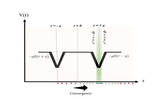
3. Swarming under the Influence of Two Delta Potential Wells

The time–independent Schrodinger’s wave equation governs the different interpretations of particle behavior:

$$[-\frac{{\mathrm{ћ}}^2}{2\mathrm{m}}{\nabla }^2+\mathrm{V}(\mathrm{r})]\mathsf{\psi }(\mathrm{r})=\mathrm{E}\mathsf{\psi }(\mathrm{r})$$

(10)

ψ(r), V(r), m, E, and $\mathrm{ћ}$ represent the wave function, the potential function, the reduced mass, the energy of the particle, and reduced Planck’s constant, respectively. However, the wave function $\mathsf{\psi }(\mathrm{r})$ has no physical significance on its own: its amplitude squared is a measure of the probability of finding a particle. Let us consider a particle under the influence of two delta potential wells experiencing an attractive potential $\mathrm{V}$:

$$\mathrm{V}(\mathrm{r})=-\mathsf{\mu }\left\{\mathsf{\delta }(\mathrm{r}+\mathrm{a})+\mathsf{\delta }(\mathrm{r}-\mathrm{a})\right\}$$

(11)

The centers of the two wells are at $-\mathrm{a}$ and $\mathrm{a}$ and $\mathsf{\mu }$ is a constant indicative of the depth of the wells. Under the assumption that the particle experiences no attractive potential, i.e., $\mathrm{V}=0$ in regions far away from the centers, the even solution of the time–independent Schrodinger’s equation in Equation (10) takes the following form:

$$-\frac{{\mathrm{ћ}}^2}{2\mathrm{m}}\frac{{\mathrm{d}}^2}{{\mathrm{dr}}^2}\mathsf{\psi }(\mathrm{r})=\mathrm{E}\mathsf{\psi }(\mathrm{r})$$

(12)

The even solutions to $\mathsf{\psi }$ for $\mathrm{E}<0$ (bound states) in regions $\mathbb{R}1:\mathrm{r}\in (-\infty ,\mathrm{a})$, $\mathbb{R}2:\mathrm{r}\in (-\mathrm{a},\mathrm{a}) \mathrm{and} \mathbb{R}3:\mathrm{r}\in (\mathrm{a},\infty )$, taking k to be equal to ($\sqrt{2\mathrm{mE}}/\mathrm{ћ}$) can be expressed as has been proved in Griffiths [15]:

$${\mathsf{\psi }}_{\mathrm{even}}\left(\mathrm{r}\right)=\{\begin{array}{cc}{\mathsf{\eta }}_1\exp \left(-\mathrm{kr}\right)\hfill & \hfill \mathrm{r}>\mathrm{a}\\ {\mathsf{\eta }}_2\exp \left(-\mathrm{kr}\right)+{\mathsf{\eta }}_3\exp \left(\mathrm{kr}\right)\hfill & \hfill 0<\mathrm{r}<\mathrm{a}\\ {\mathsf{\eta }}_2\exp \left(\mathrm{kr}\right)+{\mathsf{\eta }}_3\exp \left(-\mathrm{kr}\right)\hfill & \hfill -\mathrm{a}<\mathrm{r}<0\\ {\mathsf{\eta }}_1\exp \left(\mathrm{kr}\right)\hfill & \hfill \mathrm{r}<-\mathrm{a}\end{array}$$

(13)

The constants ${\mathsf{\eta }}_1$ and ${\mathsf{\eta }}_2$ described in the above equation are obtained by (a) solving for the continuity of the wave function ${\mathsf{\psi }}_{\mathrm{even}}$ at $\mathrm{r}=\mathrm{a}$ and $\mathrm{r}=-\mathrm{a}$ and (b) solving for the continuity of the derivative of the wave function at $\mathrm{r}=0$. Thus, ${\mathsf{\psi }}_{\mathrm{even}}$ may be rewritten below as has been in Griffiths [15].

$${\mathsf{\psi }}_{\mathrm{even}}\left(\mathrm{r}\right)=\{\begin{array}{cc}{\mathsf{\eta }}_2\left\{1+\exp \left(2\mathrm{ka}\right)\right\}\exp \left(-\mathrm{kr}\right)\hfill & \hfill \mathrm{r}>\mathrm{a}\\ {\mathsf{\eta }}_2\left\{\exp \left(-\mathrm{kr}\right)+\exp \left(\mathrm{kr}\right)\right\}\hfill & \hfill -\mathrm{a}<\mathrm{r}<\mathrm{a}\\ {\mathsf{\eta }}_2\left\{1+\exp \left(2\mathrm{ka}\right)\right\}\exp \left(\mathrm{kr}\right)\hfill & \hfill \mathrm{r}<-\mathrm{a}\end{array}$$

(14)

The odd wave function ${\mathsf{\psi }}_{\mathrm{odd}}$ does not guarantee that a solution would be found [15]. Additionally, the bound state energy in double well setup is lower than that in a single well setup by approximately a factor of ${(1.11)}^2\approx 1.2321$ [16]:

$${\mathrm{E}}_{\mathrm{bs},\mathrm{Double} \mathrm{Well}}=-{(1.11)}^2{\mathrm{E}}_{\mathrm{bs},\mathrm{Single} \mathrm{Well}}$$

(15)

To study the motional aspect of a particle its probability density function given by the squared magnitude of ${\mathsf{\psi }}_{\mathrm{even}}$ is formally expressed. Further, the claim that there is greater than 50% probability of a particle existing in neighborhood of the center of any of the potential wells (assumed centered at 0) boils down to the following criterion being met [2].

$${{\displaystyle \int }}_{-\left|\mathrm{r}\right|}^{\left|\mathrm{r}\right|}{\mathsf{\psi }}_{\mathrm{even}}{(\mathrm{r})}^2\mathrm{dr}>0.5$$

(16)

$-\left|\mathrm{r}\right|$ and $\left|\mathrm{r}\right|$ are the dynamic limits of the neighborhood. Doing away with the inequality, Equation (16) is rewritten as:

$${{\displaystyle \int }}_{-\left|\mathrm{r}\right|}^{\left|\mathrm{r}\right|}{\mathsf{\psi }}_{\mathrm{even}}{(\mathrm{r})}^2\mathrm{dr}=0.5\mathsf{\lambda }\hspace{1em}(1<\mathsf{\lambda }<2)$$

(17)

Equation (17) is the criterion for localization around the center of a potential well in a double Dirac delta well.

4. The Quantum Double Delta Swarm (QDDS) Algorithm

To ease computations, we make the assumption that one of the two potential wells is centered at 0. Then, solving for conditions of localization of the particle in the neighborhood around the center of that well and computing ${\int }_{-\left|\mathrm{r}\right|}^{\left|\mathrm{r}\right|}(\mathsf{\psi }{(\mathrm{r})}^2\mathrm{dr}$ for regions $\mathbb{R}{2}_{0-}:{\mathrm{r}}^{\prime }\in (-\mathrm{r},0)$ and $\mathbb{R}{2}_{0+}:{\mathrm{r}}^{\prime }\in (0,\mathrm{r})$, we obtain the relationship below.

$${\mathsf{\eta }}_2{}^2=\frac{\mathrm{k}\mathsf{\lambda }}{\exp (2\mathrm{kr})-5\exp (-2\mathrm{kr})+4\mathrm{kr}+4}$$

(18)

Replacing denominator of the Right Hand Side (R.H.S.) of Equation (18) i.e., ($\exp (2\mathrm{kr})-5\exp (-2\mathrm{kr})+4\mathrm{kr}+4$) as δ, we rewrite it as

$$\mathsf{\delta }=\exp (2\mathrm{kr})-5\exp (-2\mathrm{kr})+4\mathrm{kr}+4$$

(19)

Equating ${\mathrm{B}}^2$ in the Left Hand Side (L.H.S.) of Equation (18) for any two consecutive iterations (assuming it is a constant over iterations as it not a function of time) we get Equations (20)–(22):

$$\frac{{\mathsf{\lambda }}_{\mathrm{t}}}{\exp (2{\mathrm{kr}}_{\mathrm{t}})-5\exp (-2{\mathrm{kr}}_{\mathrm{t}})+4{\mathrm{kr}}_{\mathrm{t}}+4}=\frac{{\mathsf{\lambda }}_{\mathrm{t}-1}}{\exp (2{\mathrm{kr}}_{\mathrm{t}-1})-5\exp (-2{\mathrm{kr}}_{\mathrm{t}-1})+4{\mathrm{kr}}_{\mathrm{t}-1}+4}$$

(20)

$$\Rightarrow \frac{{\mathsf{\lambda }}_{\mathrm{t}}}{{\mathsf{\delta }}_{\mathrm{t}}}=\frac{{\mathsf{\lambda }}_{\mathrm{t}-1}}{{\mathsf{\delta }}_{\mathrm{t}-1}}$$

(21)

$$\Rightarrow {\mathsf{\delta }}_{\mathrm{t}}=\mathrm{\Lambda }.{\mathsf{\delta }}_{\mathrm{t}-1}\hspace{1em}\hspace{1em}\hspace{1em}(0.5<\mathrm{\Lambda }<2)$$

(22)

$\mathrm{\Lambda }$ is the ratio $({\mathsf{\lambda }}_{\mathrm{t}}/{\mathsf{\lambda }}_{\mathrm{t}-1})$ and it may vary between 0.5 to 2 since (1 < $\mathsf{\lambda }$ < 2). To keep a particle constrained within the vicinity of the center of the potential well, it must meet the following condition.

$$\frac{1}{2}{\mathsf{\delta }}_{\mathrm{t}-1}<{\mathsf{\delta }}_{\mathrm{t}}<2{\mathsf{\delta }}_{\mathrm{t}-1}$$

(23)

Thus, we find ${\mathsf{\delta }}_{\mathrm{t}}$ for any iteration by utilizing ${\mathsf{\delta }}_{\mathrm{t}-1}$, obtained in the immediately past iteration. This is done by accounting for a correction factor in the form of the gradient of ${\mathsf{\delta }}_{\mathrm{t}-1}$, multiplied by a learning rate $\mathsf{\alpha }$. The computation of ${\mathsf{\delta }}_{\mathrm{t}}$ from ${\mathsf{\delta }}_{\mathrm{t}-1}$ feeds off the relationship of ${\mathsf{\delta }}_{\mathrm{t}-1}$ with ${\mathsf{\delta }}_{\mathrm{t}-2}$ while taking the sign of the gradient of ${\mathsf{\delta }}_{\mathrm{t}-1}$ into consideration. The procedural details are outlined in Algorithm 1. The learning rate $\mathsf{\alpha }$ is chosen as a linearly decreasing, time–varying one (LTV) to help facilitate exploration of the solution space early on in the optimization phase and a gradual shift to exploitation as the process evolves. ν is a small fraction between 0 and 1 chosen at will. However, one empirically successful value is 0.3 and we use it in our computations.

$$\mathsf{\alpha }=(1-\mathsf{\nu })(\frac{\mathrm{maximum} \mathrm{number} \mathrm{of} \mathrm{iterations}-\mathrm{current} \mathrm{iteration}}{\mathrm{maximum} \mathrm{number} \mathrm{of} \mathrm{iterations}})+\mathsf{\nu }$$

(24)

Upon computing a value for ${\mathsf{\delta }}_{\mathrm{t}}$, Equation (19) is solved to retrieve an estimate of ${\mathrm{r}}_{\mathrm{t}}$, which denotes a candidate position as well as a potential solution at the end of that iteration.

$${\mathrm{r}}_{\mathrm{t}}\cong \mathrm{Solve}\left[\left\{\mathsf{\delta }-(\exp (2\mathrm{kr})-5\exp (-2\mathrm{kr})+4\mathrm{kr}+4)\right\}=0\right]$$

(25)

We let ${\mathrm{r}}_{\mathrm{t}}$, i.e., a particle’s position in the current iteration, maintain a component towards the best position found so far (gbest) in addition to its current solution obtained from Equation (19). Let $\mathsf{\rho }$ denote the component towards the gbest position and (1 − $\mathsf{\rho }$) be that towards the current solution.

$${\mathrm{r}}_{\mathrm{t}}^{\mathrm{new}}={\mathsf{\rho }\mathrm{r}}_{\mathrm{t}}+(1-\mathsf{\rho }){\mathrm{r}}_{\mathrm{gbest}}$$

(26)

A cost function is subsequently computed and the corresponding particle position is saved if the cost is lowest among all the historical swarm-wide best costs obtained. This process is repeated until the convergence criteria of choice (solution accuracy threshold, computational expense, memory requirements, success rate, etc.) are met. Figure 1 illustrates the double well potential setup.

4.1. QDDS with Chaotic Chebyshev Map (C-QDDS)

In this section, we use a Chebyshev chaotic map to generate coefficient sequences for driving the belief $\mathsf{\rho }$ in the solution update phase of the QDDS algorithm.

4.1.1. Chebyshev Map Driven Solution Update-Motivation

Chaotic metaheuristics necessitate control over the balance between diversification and intensification phases. The diversification phase is carried out by choosing an appropriate chaotic system which performs the extensive search, while the intensification phase is carried out by performing a local search such as gradient descent. It is important that during the initial progression of the search, multiple orbits pass through the vicinity of the local extrema. A large perturbation weight ensures that the strange attractor of one local extremum intersects the strange attractor of any of the other local extrema [17]. To this end, we generate a sorted sequence which acts as a perturbation source of tapering magnitude using the Chebyshev chaotic map using the recursive relation in Equation (27) [18]. There is a relative dearth of studies looking at chaotic perturbations to agent positions to drive them towards socially optimal agent locations. In our approach, we look to facilitate extensive communication among agents by employing larger chaotic weights (diversification phase) in the initial stages and local communication among agents by tapering weights (intensification phase) with the progression of function evaluations. The optimal choice and arrangement of the modulus and sign of the weights generated using the pseudo random number generator or any other method for that matter is subject to change with a change in the application problem and is very much an open question in an exploration–exploitation-based search niche. However, the two properties of ergodicity and non-repetition in chaotic time sequences have proved useful in a number of related classical studies [19,20,21] and are key factors supporting the choice of the perturbation weights in this work. Furthermore, the properties of large Lyapunov coefficient (a measure of chaoticity) and space–filling nature of the Chebyshev sequence serve to help avoid stagnation in local extrema and supplement the choice of the type of chaotic map in the studies in this article. Figure 2 and Figure 3 highlight the generated weights (${\mathsf{\rho }}^{\mathrm{Chebyshev}}$) from a Chebyshev chaotic map over 1000 iterations as well as the corresponding histogram. A schematic of the C-QDDS workflow is shown in Figure 4.

$${\mathsf{\rho }}_{\mathrm{t}}^{\mathrm{Chebyshev}}=\cos (\mathrm{t}·{\cos }^{-1}({\mathsf{\rho }}_{\mathrm{t}-1}^{\mathrm{Chebyshev}}))$$

(27)

Equation (26) subsequently becomes

$${\mathrm{r}}_{\mathrm{t}}^{\mathrm{new}}={\mathsf{\rho }}_{\mathrm{t}}^{\mathrm{Chebyshev}}\ast {\mathrm{r}}_{\mathrm{iter}}+(1-{\mathsf{\rho }}_{\mathrm{t}}^{\mathrm{Chebyshev}})\ast {\mathrm{r}}_{\mathrm{gbest}}$$

(28)

Algorithm 1. Quantum Double Delta Swarm Algorithm

4.1.2. Pseudocode of the C-QDDS Algorithm

In this section, we present the pseudocode of the Chaotic Quantum Double Delta Swarm (C-QDDS) algorithm.

5. Experimental Setup

5.1. Benchmark Functions

A suite of the following 23 optimization benchmark functions (F1–F23) are popularly used to inspect the performance of evolutionary optimization paradigms and have been utilized in this work to characterize the behavior of C-QDDS across unimodal and multimodal function landscapes of fixed and varying dimensionality.

5.2. Parameter Settings

We chose the constant k to be 5 and θ to be the product of a random number drawn from a zero-mean Gaussian distribution with a standard deviation of 0.5 and a factor of the order of 10⁻³ after sufficient number of trials. The learning rate χ decreases linearly with iterations from 1 to 0.3 according to Equation (24) as an LTV weight [8]. ${\mathsf{\rho }}^{\mathrm{Chebyshev}}\in \left[0,1\right]$ is a random number generated using a Chebyshev chaotic map in Equation (27). All experiments were carried out on two Intel(R) Core(TM) i7-5.500U CPUs @ 2.40GHz with 8GB RAM and one Intel(R) Core(TM) i7-2600U CPU @ 3.40GHz with 16GB RAM using MATLAB R2017a. All experiments were independently repeated 30 times in order to account for variability in reported data due to the underlying stochasticity of the metaheuristics used. Clusters from the MATLAB Parallel Computing Cloud were utilized to speed up the benchmarking.

6. Experimental Results

Table 1. General terms used in context of the algorithms and experimentation.

Term	Discussion
Some General Terms
Population (X)	The collection or ‘swarm’ of agents employed in the search space
Fitness Function (f)	A measure of convergence efficiency
Current Iteration	The ongoing iteration among a batch of dependent/independent runs
Maximum Iteration Count	The maximum number of times runs are to be performed
Particle Swarm Optimization (PSO)
Position (X)	Position value of individual swarm member in multidimensional space
Velocity (v)	Velocity values of individual swarm members
Cognitive Accl. Coefficient (C1)	Empirically found scale factor of pBest attractor
Social Accl. Coefficient (C2)	Empirically found scale factor of gBest attractor
Personal Best (pBest)	Position corresponding to historically best fitness for a swarm member
Global Best (gBest)	Position corresponding to best fitness over history for swarm members
Inertia Weight Coefficient (ω)	Facilitates and modulates exploration in the search space
Cognitive Random Perturbation (r1)	Random noise injector in the Personal Best attractor
Social Random Perturbation (r2)	Random noise injector in the Global Best attractor
Quantum-behaved Particle Swarm Optimization (QPSO)
Local Attractor	Set of local attractors in all dimensions
Characteristic Length	Measure of scales on which significant variations occur
Contraction–Expansion Parameter (β)	Scale factor influencing the convergence speed of QPSO
Mean Best	Mean of personal bests across all particles, akin to leader election in species
Quantum Double–Delta Swarm Optimization (QDDS)
$\mathsf{\rho }$	Component towards the global best position gbest
$\mathsf{\psi }(\mathrm{r})$	Wave function in the Schrodinger’s equation
${\mathsf{\psi }}_{\mathrm{even}}(\mathrm{r})$	Even solutions to Schrodinger’s Equation for Double Delta Potential Well
$\mathrm{V}(\mathrm{r})$	Potential Function
$\mathrm{\Lambda }$	Limiter
${\mathsf{\delta }}_{\mathrm{iter}}$	Characteristic Constraint
$\mathrm{\epsilon }$	A small fraction between 0 and 1 chosen at will
$\mathbb{R}1:\mathrm{r}\in (-\infty ,\mathrm{a})$	Region 1
$\mathbb{R}2:\mathrm{r}\in (-\mathrm{a},\mathrm{a})$	Region 2
$\mathbb{R}3:\mathrm{r}\in (\mathrm{a},\infty )$	Region 3
$\mathsf{\alpha }$	Learning Rate
${\mathsf{\rho }}_{\mathrm{iter}}^{\mathrm{Chebyshev}}$	Component towards global best gbest drawn from Chebyshev map
$\mathsf{\mu }$	Depth of the wells
$\mathrm{a}$	Coordinate of wells

introduces some general terms used in context of the algorithms and experimentation,

Table 2. Unimodal test functions considered for testing.

Number	Name	Expression	Range	Min
F1	Sphere	$\mathrm{f}(\mathrm{x})={\displaystyle {\displaystyle \sum }_{\mathrm{i}=1}^{\mathrm{n}}}{\mathrm{x}}_{\mathrm{i}}^2$	[−100, 100]	f(x*) = 0
F2	Schwefel’s Problem 2.22	$\mathrm{f}(\mathrm{x})={\displaystyle {\displaystyle \sum }_{\mathrm{i}=1}^{\mathrm{n}}}\left|{\mathrm{x}}_{\mathrm{i}}\right|+{\displaystyle {\displaystyle \prod }_{\mathrm{i}=1}^{\mathrm{n}}}\left|{\mathrm{x}}_{\mathrm{i}}\right|$	[−10, 10]	f(x*) = 0
F3	Schwefel’s Problem 1.2	$\mathrm{f}(\mathrm{x})={\displaystyle {\displaystyle \sum }_{\mathrm{i}=1}^{\mathrm{n}}}{\left({\displaystyle {\displaystyle \sum }_{\mathrm{j}=1}^{\mathrm{i}}}{\mathrm{x}}_{\mathrm{j}}\right)}^2$	[−100, 100]	f(x*) = 0
F4	Schwefel’s Problem 2.21	$\mathrm{f}(\mathrm{x})={\max }_{\mathrm{i}}\left\{\left|{\mathrm{x}}_{\mathrm{i}}\right|,1\le \mathrm{i}\le \mathrm{n}\right\}$	[−100, 100]	f(x*) = 0
F5	Generalized Rosenbrock’s Function	$\mathrm{f}(\mathrm{x})={\displaystyle {\displaystyle \sum }_{\mathrm{i}=1}^{\mathrm{n}-1}}\left[100{({\mathrm{x}}_{\mathrm{i}+1}-{\mathrm{x}}_{\mathrm{i}}^2)}^2+{({\mathrm{x}}_{\mathrm{i}}-1)}^2\right]$	[−n, n]	f(x*) = 0
F6	Step Function	$\mathrm{f}(\mathrm{x})={\displaystyle {\displaystyle \sum }_{\mathrm{i}=1}^{\mathrm{n}}}{(\lfloor {\mathrm{x}}_{\mathrm{i}}+0.5\rfloor )}^2$	[−100, 100]	f(x*) = 0
F7	Quartic Function i.e., Noise	$\mathrm{f}(\mathrm{x})={\displaystyle {\displaystyle \sum }_{\mathrm{i}=1}^{\mathrm{n}}}{\mathrm{ix}}^4+\mathrm{random} [0,1)$	[−1.28, 1.28]	f(x*) = 0

Note: x* Globally optimum argument.

,

Table 3. Multimodal test functions considered for testing.

Number	Name	Expression	Range	Min
F8	Generalized Schwefel’s Problem 2.26	$\mathrm{f}(\mathrm{x})=-{\displaystyle {\displaystyle \sum }_{\mathrm{i}=1}^{\mathrm{n}}}({\mathrm{x}}_{\mathrm{i}}\sin (\sqrt{\left|{\mathrm{x}}_{\mathrm{i}}\right|}))$	[−500, 500]	f(x*) = −12,569.5
F9	Generalized Rastrigrin’s Function	$\mathrm{f}(\mathrm{x})=\mathrm{An}+{\displaystyle {\sum }_{\mathrm{i}=1}^{\mathrm{n}}}\left[{\mathrm{x}}_{\mathrm{i}}{}^2-\mathrm{Acos}(2{\mathsf{\pi }\mathrm{x}}_{\mathrm{i}})\right]$, A = 10	[−5.12, 5.12]	f(x*) = 0
F10	Ackley’s Function	$\mathrm{f}(\mathrm{x})=-20\exp (-0.2\sqrt{\frac{1}{\mathrm{d}}{\displaystyle {\displaystyle \sum }_{\mathrm{i}=1}^{\mathrm{d}}}{\mathrm{x}}_{\mathrm{i}}^2})-\exp (\sqrt{\frac{1}{\mathrm{d}}{\displaystyle {\displaystyle \sum }_{\mathrm{i}=1}^{\mathrm{d}}}\cos (2{\mathsf{\pi }\mathrm{x}}_{\mathrm{i}})})+20+\exp (1)$	[−32.768, 32.768]	f(x*) = 0
F11	Generalized Griewank Function	$\mathrm{f}(\mathrm{x})=1+\frac{1}{4000}{\displaystyle {\displaystyle \sum }_{\mathrm{i}=1}^{\mathrm{n}}}{\mathrm{x}}_{\mathrm{i}}^2-{\displaystyle {\displaystyle \prod }_{\mathrm{i}=1}^{\mathrm{n}}}\cos (\frac{{\mathrm{x}}_{\mathrm{i}}}{\sqrt{\mathrm{i}}})$	[−600, 600]	f(x*) = 0
F12	Generalized Penalized Function 1	$\mathrm{f}(\mathrm{x})=\frac{\mathsf{\pi }}{\mathrm{d}}\left\{10{\sin }^2({\mathsf{\pi }\mathrm{y}}_1)+{\displaystyle {\displaystyle \sum }_{\mathrm{i}=1}^{\mathrm{n}-1}}{({\mathrm{y}}_{\mathrm{i}}-1)}^2\left[1+10{\sin }^2({\mathsf{\pi }\mathrm{y}}_{\mathrm{i}+1})+{({\mathrm{y}}_{\mathrm{n}}-1)}^2\right]+{\displaystyle {\displaystyle \sum }_{\mathrm{i}=1}^{\mathrm{n}}}\mathrm{u}({\mathrm{x}}_{\mathrm{i}},10,100,4)\right\}$	[−50, 50]	f(x*) = 0
F13	Generalized Penalized Function 2	$\mathrm{f}(\mathrm{x})=0.1\left\{\begin{array}{c}{\sin }^2(3{\mathsf{\pi }\mathrm{x}}_1)\\ +{\displaystyle {\displaystyle \sum }_{\mathrm{i}=1}^{\mathrm{n}-1}}{({\mathrm{x}}_{\mathrm{i}}-1)}^2\left[1+{\sin }^2(3{\mathsf{\pi }\mathrm{x}}_{\mathrm{i}+1})\right]+{({\mathrm{x}}_{\mathrm{n}}-1)}^2\left[1+{\sin }^2(2{\mathsf{\pi }\mathrm{x}}_{30})\right]\\ +{\displaystyle {\displaystyle \sum }_{\mathrm{i}=1}^{\mathrm{n}}}\mathrm{u}({\mathrm{x}}_{\mathrm{i}},5,100,4)\end{array}\right\}$ where $\mathrm{u}({\mathrm{x}}_{\mathrm{i}},5,100,4)=\{\begin{array}{cc}\mathrm{k}{({\mathrm{x}}_{\mathrm{i}}-\mathrm{a})}^{\mathrm{m}},\hfill & \hfill {\mathrm{x}}_{\mathrm{i}}>a\\ 0,\hfill & \hfill -a<{\mathrm{x}}_{\mathrm{i}}<a\\ \mathrm{k}{(-{\mathrm{x}}_{\mathrm{i}}-\mathrm{a})}^{\mathrm{m}},\hfill & \hfill {\mathrm{x}}_{\mathrm{i}}<-a\end{array}$ ${\mathrm{y}}_{\mathrm{i}}=1+\frac{1}{4}({\mathrm{x}}_{\mathrm{i}}+1)$	[−50, 50]	f(x*) = 0

Note: x* Globally optimum argument.

,

Table 4. Multimodal test functions with fixed dimensions considered for testing.

Number	Name	Expression	Range	Min
F14, n = 2	Shekel’s Foxholes Function	$\mathrm{f}(\mathrm{x})={\left[\frac{1}{500}+{\displaystyle {\displaystyle \sum }_{\mathrm{j}=1}^{25}}\frac{1}{\mathrm{j}+{\sum }_{\mathrm{i}=1}^2{({\mathrm{x}}_{\mathrm{i}}-{\mathrm{a}}_{\mathrm{ij}})}^6}\right]}^{-1}$ where ${\mathrm{a}}_{\mathrm{ij}}=\left(\begin{array}{cccccccccc}-32& -16& 0& 16& 32& -32& \dots & 0& 16& 32\\ -32& -32& -32& -32& -32& -16& \dots & 32& 32& 32\end{array}\right)$	[−65.536, 65.536]	f(x*) ≈ 1
F15, n = 4	Kowalik’s Function	$\mathrm{f}(\mathrm{x})={\left[{\displaystyle {\displaystyle \sum }_{\mathrm{i}=1}^{11}}{\mathrm{a}}_{\mathrm{i}}-\frac{{\mathrm{x}}_1({\mathrm{b}}_{\mathrm{i}}{}^2+{\mathrm{b}}_{\mathrm{i}}{\mathrm{x}}_2)}{{\mathrm{b}}_{\mathrm{i}}{}^2+{\mathrm{b}}_{\mathrm{i}}{\mathrm{x}}_3+{\mathrm{x}}_4}\right]}^2$ Coefficients are defined according to Table F15.	[−5, 5]	f(x*) ≈ 0.0003075
F16, n = 2	Six-Hump Camel-Back Function	$\mathrm{f}(\mathrm{x})=4{\mathrm{x}}_1{}^2-2.1{\mathrm{x}}_1{}^4+\frac{1}{3}{\mathrm{x}}_1{}^6+{\mathrm{x}}_1{\mathrm{x}}_2-4{\mathrm{x}}_2{}^2+4{\mathrm{x}}_2{}^4$	[−5, 5]	f(x*) = −1.0316285
F17, n = 2	Branin Function	$\mathrm{f}(\mathrm{x})={\left({\mathrm{x}}_2-\frac{5.1}{4{\mathsf{\pi }}^2}{\mathrm{x}}_1{}^2+\frac{5}{\mathsf{\pi }}{\mathrm{x}}_1-6\right)}^2+10\left(1-\frac{1}{8\mathsf{\pi }}\right){\cos \mathrm{x}}_1+10$	$-5\le {\mathrm{x}}_1\le 10$, $0\le {\mathrm{x}}_2\le 15$	f(x*) = 0.398
F18, n = 2	Goldstein-Price Function	$$\begin{gathered} \mathrm{f}(\mathrm{x})=\left[1+{({\mathrm{x}}_1+{\mathrm{x}}_2+1)}^2(19-14{\mathrm{x}}_1+3{\mathrm{x}}_1{}^2-14{\mathrm{x}}_2+6{\mathrm{x}}_1{\mathrm{x}}_2+3{\mathrm{x}}_2{}^2)\right] \\ \left[30+{(2{\mathrm{x}}_1-3{\mathrm{x}}_2)}^2(18-32{\mathrm{x}}_1+12{\mathrm{x}}_1{}^2+48{\mathrm{x}}_2-36{\mathrm{x}}_1{\mathrm{x}}_2+27{\mathrm{x}}_2{}^2)\right] \end{gathered}$$	[−2, 2]	f(x*) = 3
F19, n = 3	Hartman’s Family Function 1	$\mathrm{f}(\mathrm{x})=-{\displaystyle {\displaystyle \sum }_{\mathrm{i}=1}^4}{\mathrm{c}}_{\mathrm{i}}\exp \left[-{\displaystyle {\displaystyle \sum }_{\mathrm{j}=1}^3}{\mathrm{a}}_{\mathrm{ij}}{({\mathrm{x}}_{\mathrm{j}}-{\mathrm{p}}_{\mathrm{ij}})}^2\right]$	$0\le {\mathrm{x}}_{\mathrm{j}}\le 1$	f(x*) = −3.86
F20, n = 6	Hartman’s Family Function 2	$\mathrm{f}(\mathrm{x})=-{\displaystyle {\displaystyle \sum }_{\mathrm{i}=1}^4}{\mathrm{c}}_{\mathrm{i}}\exp \left[-{\displaystyle {\displaystyle \sum }_{\mathrm{j}=1}^6}{\mathrm{a}}_{\mathrm{ij}}{({\mathrm{x}}_{\mathrm{j}}-{\mathrm{p}}_{\mathrm{ij}})}^2\right]$ Coefficients are defined according to Table F20.1 and F20.2 respectively.	$0\le {\mathrm{x}}_{\mathrm{j}}\le 1$	f(x*) = −3.86
F21, n = 4	Shekel’s Family Function 1	$\mathrm{f}(\mathrm{x})=-{\displaystyle {\displaystyle \sum }_{\mathrm{i}=1}^5}{\left[(\mathrm{x}-{\mathrm{a}}_{\mathrm{i}}){(\mathrm{x}-{\mathrm{a}}_{\mathrm{i}})}^{\mathrm{T}}+{\mathrm{c}}_{\mathrm{i}}\right]}^{-1}$ Coefficients are defined according to Table F21.	$0\le {\mathrm{x}}_{\mathrm{j}}\le 10$	$\mathrm{f}({\mathrm{x}}_{\mathrm{local}}^{\ast })=\frac{1}{{\mathrm{c}}_{\mathrm{i}}},$ $1\le \mathrm{i}\le \mathrm{m}$
F22, n = 4	Shekel’s Family Function 2	$\mathrm{f}(\mathrm{x})=-{\displaystyle {\displaystyle \sum }_{\mathrm{i}=1}^7}{\left[(\mathrm{x}-{\mathrm{a}}_{\mathrm{i}}){(\mathrm{x}-{\mathrm{a}}_{\mathrm{i}})}^{\mathrm{T}}+{\mathrm{c}}_{\mathrm{i}}\right]}^{-1}$ Coefficients are defined according to Table F22.	$0\le {\mathrm{x}}_{\mathrm{j}}\le 10$	$\mathrm{f}({\mathrm{x}}_{\mathrm{local}}^{\ast })=\frac{1}{{\mathrm{c}}_{\mathrm{i}}},$ $1\le \mathrm{i}\le \mathrm{m}$
F23, n = 4	Shekel’s Family Function 3	$\mathrm{f}(\mathrm{x})=-{\displaystyle {\displaystyle \sum }_{\mathrm{i}=1}^{10}}{\left[(\mathrm{x}-{\mathrm{a}}_{\mathrm{i}}){(\mathrm{x}-{\mathrm{a}}_{\mathrm{i}})}^{\mathrm{T}}+{\mathrm{c}}_{\mathrm{i}}\right]}^{-1}$ Coefficients are defined according to Table F23.	$0\le {\mathrm{x}}_{\mathrm{j}}\le 10$	$\mathrm{f}({\mathrm{x}}_{\mathrm{local}}^{\ast })=\frac{1}{{\mathrm{c}}_{\mathrm{i}}},$ $1\le \mathrm{i}\le \mathrm{m}$

Note: x* Globally optimum argument, x*_local Locally optimum argument.

,

Table 5. Coefficients of Kowalik’s Function (F15).

Index (i)	${\mathbf{a}}_{\mathbf{i}}$	${\mathbf{a}}_{\mathbf{ij}}{}^{-1}$
1	0.1957	0.25
2	0.1947	0.5
3	0.1735	1
4	0.1600	2
5	0.0844	4
6	0.0627	6
7	0.0456	8
8	0.0342	10
9	0.0323	12
10	0.0235	14
11	0.0246	16

,

Table 6. Coefficients of Hartman’s Functions (F19).

Index (i)	${\mathbf{a}}_{\mathbf{ij}}, \mathbf{j}=1,2,3$			${\mathbf{c}}_{\mathbf{i}}$	${\mathbf{p}}_{\mathbf{i}\mathbf{j}}, \mathbf{j}=1,2,3$
1	3	10	30	1	0.3689	0.1170	0.2673
2	0.1	10	35	1.2	0.4699	0.4387	0.7470
3	3	10	30	3	0.1091	0.8732	0.5547
4	0.1	10	35	3.2	0.038150	0.5743	0.8828

,

Table 7. Coefficients of Hartman’s Functions (F20).

Index (i)	${\mathbf{a}}_{\mathbf{i}\mathbf{j}}, \mathbf{j}=1,2,3$						${\mathbf{c}}_{\mathbf{i}}$	${\mathbf{p}}_{\mathbf{i}\mathbf{j}}, \mathbf{j}=1,2,3$
1	10	3	17	3.5	1.7	8	1	0.1312	0.1696	0.5569	0.0124	0.8283	0.5886
2	0.5	10	17	0.1	8	14	1.2	0.2329	0.4135	0.8307	0.3736	0.1004	0.9991
3	3	3.5	1.7	10	17	8	3	0.2348	0.1415	0.3522	0.2883	0.3047	0.6650
4	17	8	0.05	10	0.1	14	3.2	0.4047	0.8828	0.8732	0.5743	0.1091	0.0381

and

Table 8. Coefficients of Shekel’s Functions (F21–F23).

Index (i)	${\mathbf{a}}_{\mathbf{i}\mathbf{j}}, \mathbf{j}=1,\dots ,4$				${\mathbf{c}}_{\mathbf{i}}$
1	4	4	4	4	0.1
2	1	1	1	1	0.2
3	8	8	8	8	0.4
4	6	6	6	6	0.4
5	3	7	3	7	0.4
6	2	9	2	9	0.6
7	5	5	3	3	0.3
8	8	1	8	1	0.7
9	6	2	6	2	0.5
10	7	3.6	7	3.6	0.5

provide a detailed listing of the benchmark functions under consideration and

Table 9. 3D Surface Plots of the Benchmark Functions F1–F23.

provide the 3D plots of these functions, whereas

Table 10. Solution quality in unimodal functions in Table 2 (30D, 1000 iterations, 30 independent trials).

Fn	Stat	C-QDDS Chebyshev Map	Sine Cosine Algorithm	Dragon Fly Algorithm	Ant Lion Optimization	Whale Optimization	Firefly Algorithm	QPSO	PSO w = 0.95*w	PSO No Damping
F1	Mean	1.1956 × 10−6	0.0055	469.8818	7.8722 × 10−7	17.3824	3.5794 × 104	3.0365 × 103	109.5486	110.3989
	Min	5.1834 × 10−7	1.0207 × 10−7	23.9914	8.9065 × 10−8	0.6731	3.0236 × 104	1.3286 × 103	39.3329	42.8825
	Std	2.8711 × 10−7	0.0161	474.0822	1.0286 × 10−6	19.6687	3.3373 × 103	920.4817	43.3127	54.7791
F2	Mean	0.0051	3.6862 × 10−6	9.2230	27.8542	0.7846	3.4566 × 104	36.4162	4.2299	4.4102
	Min	0.0025	2.7521 × 10−9	0	0.0029	0.0745	84.8978	21.7082	2.0290	2.1627
	Std	9.7281 × 10−4	8.9681 × 10−6	5.7226	42.2856	0.5303	1.3595 × 105	12.5312	1.1111	1.3804
F3	Mean	1.0265 × 10−4	3.4383 × 103	6.3065 × 103	302.3783	1.0734 × 105	4.4017 × 104	3.0781 × 104	4.0409 × 103	3.4218 × 103
	Min	1.0184 × 10−5	27.3442	310.7558	102.7732	5.0661 × 104	3.0021 × 104	1.8940 × 104	2.2416 × 103	1.9223 × 103
	Std	6.5905 × 10−5	3.1641 × 103	4.7838 × 103	167.7687	4.0661 × 104	6.6498 × 103	5.9848 × 103	994.2550	997.4284
F4	Mean	3.6945 × 10−4	12.8867	13.8222	8.8157	66.4261	68.4102	56.5926	12.8272	11.9252
	Min	1.4162 × 10−4	1.4477	4.1775	2.0212	17.8904	62.9296	32.6744	10.2302	9.0857
	Std	9.8034 × 10−5	8.1625	5.5197	3.0808	21.5187	2.6497	8.2985	1.5793	2.0508
F5	Mean	28.7211	60.7787	2.0123 × 104	143.9657	1.5976 × 103	7.4584 × 107	2.1204 × 106	6.0590 × 103	5.3377 × 103
	Min	28.7074	28.0932	44.0682	20.7989	39.9132	3.8917 × 107	5.0759 × 105	655.5618	1.2610 × 103
	Std	0.0077	55.2793	3.6793 × 104	288.1879	3.0458 × 103	2.0606 × 107	9.1390 × 105	4.2558 × 103	2.6303 × 103
F6	Mean	7.2332	4.2963	488.3942	6.0117 × 10−7	30.0158	3.6216 × 104	3.6028 × 103	107.5196	116.9431
	Min	6.4389	3.3201	17.4978	8.9390 × 10−8	0.8531	2.8838 × 104	1.8380 × 103	45.9374	28.9258
	Std	0.5612	0.4007	309.2795	6.2634 × 10−7	44.1595	2.8434 × 103	986.7972	47.5633	49.5767
F7	Mean	0.0037	0.0289	0.1491	0.0541	0.1265	36.0335	1.4761	0.1737	0.1749
	Min	4.9685 × 10−4	0.0010	0.0157	0.0210	0.0177	21.1334	0.3837	0.0697	0.0734
	Std	0.0023	0.0472	0.0918	0.0229	0.0993	7.5632	0.7718	0.0561	0.0690

,

Table 11. Solution quality in multimodal functions in Table 3 (30D, 1000 iterations, 30 independent trials).

Fn	Stat	C-QDDS Chebyshev Map	Sine Cosine Algorithm	Dragon Fly Algorithm	Ant Lion Optimizer	Whale Optimization	Firefly Algorithm	QPSO	PSO w = 0.95*w	PSO No Damping
F8	Mean	−602.2041	−4.0397 × 103	−6.001 × 103	−5.5942 × 103	−8.5061 × 103	−3.8714 × 103	−3.3658 × 103	−5.1487 × 103	−4.8821 × 103
	Best	−975.5422	−4.4739 × 103	−8.9104 × 103	−8.2843 × 103	−1.0768 × 104	−4.2603 × 103	−5.0298 × 103	−7.4208 × 103	−6.6643 × 103
	Std	160.8409	214.0523	783.7255	515.1599	895.4642	204.0029	486.0400	766.3330	750.3092
F9	Mean	2.4873 × 10−4	8.8907	124.0432	79.9945	116.4796	328.4011	248.0831	57.8114	57.1125
	Best	8.2194 × 10−5	1.0581 × 10−6	32.1699	45.7681	0.4305	308.3590	177.8681	19.1318	27.4985
	Std	6.3770 × 10−5	16.2284	40.4730	22.2932	88.0344	10.1050	31.9501	15.1644	15.0292
F10	Mean	8.1297 × 10−4	10.7873	6.0693	1.6480	1.1419	19.3393	12.3433	4.9951	4.9271
	Best	5.6777 × 10−4	3.4267 × 10−5	8.8818 × 10−16	1.7296 × 10−4	0.0265	18.4515	9.7835	3.9874	2.9208
	Std	8.8526 × 10−5	9.6938	1.9141	0.9544	0.9926	0.2797	1.8413	0.6230	0.7957
F11	Mean	8.7473 × 10−8	0.1770	5.0784	0.0082	1.1735	316.5026	33.5446	2.0669	2.0604
	Best	3.5705 × 10−8	2.2966 × 10−5	1.1727	2.5498 × 10−5	0.9839	226.5205	11.9701	1.3636	1.3744
	Std	2.6504 × 10−8	0.2195	4.5098	0.0093	0.2340	33.3806	12.5605	0.5989	0.5366
F12	Mean	0.0995	991.4301	12.2571	9.4380	642.0404	1.2629 × 108	5.6147 × 105	6.4329	6.5610
	Best	0	0.2878	1.6755	3.4007	0.0442	5.6104 × 107	4.0841 × 104	1.0266	2.8742
	Std	0.2621	5.4201 × 103	13.5218	3.9121	3.5039 × 103	4.4034 × 107	6.9761 × 105	2.7882	3.0003
F13	Mean	0.0105	3.1940	1.5156 × 104	0.0133	2.3405 × 103	2.8867 × 108	3.5568 × 106	38.1945	39.0369
	Best	0	1.8776	5.6609	2.7212 × 10−7	0.3813	1.3101 × 108	6.8216 × 105	12.7653	15.4619
	Std	0.0576	2.2922	6.0811 × 104	0.0163	1.2373 × 104	8.1766 × 107	2.4393 × 106	15.2922	27.6751

and

Table 12. Solution quality in multimodal functions in Table 4 (fixed dim, 1000 iterations, 30 trials).

Fn	Stat	C-QDDS Chebyshev Map	Sine Cosine Algorithm	Dragon Fly Algorithm	Ant Lion Optimizer	Whale Optimization	Firefly Algorithm	QPSO	PSO w = 0.95*w	PSO No Damping
F14, n = 2	Mean	3.6771	1.3949	1.0311	1.2299	4.2524	1.0519	2.3561	2.7786	3.7082
	Best	1.0056	0.9980	0.9980	0.9980	0.9980	0.9980	0.9981	0.9980	0.9980
	Std	2.2295	0.8072	0.1815	0.4276	3.7335	0.1889	1.7188	2.2246	2.7536
F15, n = 4	Mean	3.7361 × 10−4	9.1075 × 10−4	0.0016	0.0027	0.0051	0.0024	0.0030	0.0036	0.0034
	Best	3.1068 × 10−4	3.1549 × 10−4	4.7829 × 10−4	4.0518 × 10−4	3.4820 × 10−4	0.0011	7.2169 × 10−4	3.6642 × 10−4	3.0858 × 10−4
	Std	5.0123 × 10−5	4.2242 × 10−4	0.0014	0.0060	0.0076	0.0012	0.0059	0.0063	0.0068
F16, n = 2	Mean	−0.5487	−1.0316	−1.0316	−1.0316	−1.0315	−1.0295	−1.0316	−1.0316	−1.0316
	Best	−1.0315	−1.0316	−1.0316	−1.0316	−1.0316	−1.0316	−1.0316	−1.0316	−1.0316
	Std	0.4275	1.1863 × 10−5	1.4229 × 10−6	3.6950 × 10−14	3.3613 × 10−4	0.0030	1.1009 × 10−4	8.2108	2.7251 × 10−13
F17, n = 2	Mean	0.4721	0.3983	0.3979	0.3979	0.4069	0.4002	0.4000	0.3979	0.3979
	Best	0.3989	0.3979	0.3979	0.3979	0.3979	0.3979	0.3979	0.3979	0.3979
	Std	0.0920	4.8435 × 10−4	4.9327 × 10−8	2.3588 × 10−14	0.0179	0.0020	0.0043	5.0770 × 10−10	2.1067 × 10−8
F18, n = 2	Mean	3.8438	3	3	3	3.9278	3.0402	3.0007	3.0000	3.0000
	Best	3.0080	3	3	3	3.0000	3.0002	3.0000	3.0000	3.0000
	Std	0.9128	5.7657 × 10−6	8.7817 × 10−7	1.2869 × 10−13	5.0752	0.0397	0.0017	1.0155 × 10−11	5.8511 × 10−11
F19, n = 3	Mean	−3.6805	−3.8547	−3.8625	−3.8628	−3.8246	−3.8542	−3.8628	−3.8628	−3.8628
	Best	−3.8587	−3.8626	−3.8628	−3.8628	−3.8628	−3.8625	−3.8628	−3.8628	−3.8628
	Std	0.1942	0.0016	8.8455 × 10−4	7.5193 × 10−15	0.0657	0.0066	1.5043 × 10−5	5.2841 × 10−11	9.2140 × 10−11
F20, n = 6	Mean	−2.2207	−2.9961	−3.2421	−3.2705	−3.0966	−3.0645	−3.2646	−3.2625	−3.2546
	Best	−2.7562	−3.2911	−3.3220	−3.3220	−3.2610	−3.2436	−3.3219	−3.3220	−3.3220
	Std	0.29884	0.2060	0.0670	0.0599	0.1535	0.0911	0.0605	0.0605	0.0599
F21, n = 4	Mean	−3.1126	−4.0962	−9.0360	−6.7752	−6.5291	−4.3198	−5.8537	−5.3955	−5.4045
	Best	−4.5610	−5.3343	−10.1532	−10.1532	−9.8465	−7.5958	−10.1474	−10.1532	−10.1532
	Std	0.7090	1.5519	1.9130	2.6824	1.9988	1.4599	3.5651	3.3029	3.4897
F22, n = 4	Mean	−3.2009	−3.9949	−10.0455	−7.2979	−6.3611	−4.2776	−6.7830	−5.3236	−6.3098
	Best	−4.5933	−7.9241	−10.4029	−10.4029	−10.2432	−9.2741	−10.3974	−10.4029	−10.4029
	Std	0.7098	2.1774	1.3422	3.0440	2.3852	1.6527	3.5783	3.2000	3.4602
F23, n = 4	Mean	−2.3595	−4.6650	−9.9928	−7.1691	−5.2592	−4.6959	−7.5372	−7.3175	−5.1501
	Best	−4.2043	−7.7259	−10.5364	−10.5364	−10.0617	−8.5734	−10.5344	−10.5364	−10.5364
	Std	0.8183	1.5038	1.6439	3.2926	2.5389	1.4647	3.6778	3.7753	3.4033

report performances of the C-QDDS algorithm on the test problems stacked against solution qualities obtained using eight other commonly used, recent nature–inspired approaches: (i) Sine Cosine Algorithm (SCA) [22], (ii) Dragon Fly Algorithm (DFA) [23], (iii) Ant Lion Optimization (ALO) [24], (iv) Whale Optimization Algorithm (WOA) [25], (v) Firefly Algorithm (FA) [26], (vi) Quantum-behaved Particle Swarm Optimization (QPSO) [2,3], (vii) Particle Swarm Optimization with Damped Inertia (** PSO-I), and (viii) the canonical Particle Swarm Optimizer (PSO-II) [6]. Each algorithm has been executed for 1000 iterations with 30 independent trials following which their mean, standard deviation, and minimum values are noted. The testing procedures carried out on the 23 functions adhere to the dimensionalities and range constraints specified in Table 2, Table 3, Table 4, Table 5, Table 6, Table 7 and Table 8 and the 3D plots of these functions were shown in Table 9. A total of 50 agents have been introduced in the particle pool, out of which only one agent is picked in each iteration. The rationale for choosing one agent instead of many or all from the pool is to investigate the incremental effect of a single agent’s propagation under different nature–inspired dynamical perturbations. The ripple effect caused otherwise, by many sensor reading exchanges among many or all particles, may be delayed when a single particle affects the global pool of particles in one iteration.

** PSO-I utilizes an exponentially decaying inertia weight for exploration–exploitation trade–off.

Test Results on Optimization Problems

7. Analysis of Experimental Results

Table 10, Table 11 and Table 12 report the solution qualities obtained on the suite of test functions F1–F23 followed by

Table 13. Win/tie/loss count among competitors w.r.t. reported global best.

Performance	Metric	C-QDDS Chebyshev Map	Sine Cosine Algorithm	Dragon Fly Algorithm	Ant Lion Optimizer	Whale Optimization	Firefly Algorithm	QPSO	PSO w = 0.95*w	PSO No Damping
Win	Mean	10	1	3	3	1	0	0	0	0
	Best	6	1	2	3	1	0	0	0	1
	Std	14	1	1	7	0	0	0	0	0
Tie	Mean	0	2	3	4	0	0	2	4	5
	Best	0	4	9	9	5	3	4	9	9
	Std	0	0	0	0	0	0	0	0	0
Lose	Mean	13	20	17	17	22	23	21	19	18
	Best	17	18	12	13	18	20	19	14	13
	Std	9	22	22	17	23	23	23	23	23

,

Table 14. Average ranks based on win/tie/loss count among competitors w.r.t. reported global best.

Performance	Metric	C-QDDS Chebyshev Map	Sine Cosine Algorithm	Dragon Fly Algorithm	Ant Lion Optimizer	Whale Optimization	Firefly Algorithm	QPSO	PSO w = 0.95*w	PSO No Damping
Win	Mean	1	3	2	2	3	4	4	4	4
	Best	1	4	3	2	4	5	5	5	4
	Std	1	3	3	2	4	4	4	4	4
Tie	Mean	5	4	3	2	5	5	4	2	1
	Best	5	3	2	2	3	4	3	2	1
	Std	1	1	1	1	1	1	1	1	1
Lose	Mean	1	5	2	2	7	8	6	4	3
	Best	4	5	1	2	5	7	6	3	2
	Std	1	3	3	2	4	4	4	4	3
Average Rank	Mean	2.333	4	2.333	2	5	5.666	4.666	3.333	2.666
	Best	3.333	4	2	2	4	5.333	4.666	3.333	2.333
	Std	1	2.333	2.333	1.666	3	3	3	3	2.666

,

Table 15. Results of two-tailed t-test for C-QDDS vs. competitors.

Algorithm	C-QDDS vs. SCA	C-QDDS vs. DFA	C-QDDS vs. ALO	C-QDDS vs. WOA	C-QDDS vs. FA	C-QDDS vs. QPSO	C-QDDS vs. PSO-II	C-QDDS vs. PSO-I
Function	t values (tcritical = 2.001717). Null Hypothesis: (µ_CQDDS − µ_Competitor) > 0
F1	−1.8707	−5.4287	2.094532	−4.84055	−5.8.7456	−18.0684	−13.8533	−11.0385
F2	28.69263	−8.82265	−3.60728	−8.05108	−1.39261	−15.9148	−20.8264	−17.4788
F3	−5.95188	−7.22065	−9.87189	−14.4592	−36.2554	−28.1704	−22.2608	−18.7903
F4	−8.64702	−13.7155	−15.6724	−16.9076	−141.411	−37.3523	−44.4852	−31.8485
F5	−3.17636	−2.99135	−2.19031	−2.8213	−19.825	−12.7079	−7.76098	−11.0552
F6	23.32769	−8.52117	70.59491	−2.82556	−69.7487	−19.9572	−11.5478	−12.12
F7	−2.92082	−8.67254	−11.9943	−6.77163	−26.0926	−10.4491	−16.5837	−13.5823
F8	70.32003	36.96027	50.66345	47.58374	68.92735	29.56635	31.80233	30.54904
F9	−3.0006	−16.7868	−19.6538	−7.24698	−178.004	−42.529	−20.8808	−20.8139
F10	−6.09462	−17.3651	−9.45308	−6.29659	−378.696	−36.7146	−43.9082	−33.9102
F11	−4.41671	−6.1678	−4.82933	−27.4681	−5.1.933	−14.6277	−18.9028	−21.0311
F12	−1.00178	−4.92371	−13.0453	−1.00347	−15.7087	−4.40833	−12.3869	−11.7511
F13	−7.60459	−1.36509	−0.25619	−1.03608	−19.337	−7.98647	−13.6763	−7.72376
F14	5.271808	6.47901	5.904436	−0.72462	6.426319	2.570191	1.562548	−0.04808
F15	−6.9162	−4.79494	−2.12362	−3.40618	−9.2411	−2.4381	−2.80494	−2.43761
F16	6.187023	6.187023	6.187023	6.18574	6.159965	6.187023	6.187023	6.187023
F17	4.393627	4.417501	4.417501	3.810236	4.27956	4.287797	4.417501	4.417501
F18	5.063193	5.063193	5.063193	−0.08922	4.81742	5.058984	5.063193	5.063193
F19	4.912978	5.133083	5.141597	3.849854	4.896216	5.141597	5.141597	5.141597
F20	11.70106	18.26704	18.86578	14.28008	14.7933	18.75247	18.71474	18.58005
F21	3.157566	15.90258	7.230404	8.823441	4.074111	4.13039	3.701433	3.525209
F22	1.898948	24.69127	7.179345	6.955444	3.278706	5.378252	3.547072	4.820763
F23	7.375911	22.76815	7.76455	5.953976	7.627314	7.526917	7.029854	4.366702
Significantly better	9	12	10	11	12	13	13	13
Significantly worse	11	10	12	8	10	10	9	9

,

Table 16. Cohen’s d-values for C-QDDS v/s competitors.

Algorithm	C-QDDS vs. SCA	C-QDDS vs. DFA	C-QDDS vs. ALO	C-QDDS vs. WOA	C-QDDS vs. FA	C-QDDS vs. QPSO	C-QDDS vs. PSO-II	C-QDDS vs. PSO-I
Function	Cohen’s d-values, where d = $\frac{{\mathsf{\mu }}_{\mathbf{C}-\mathbf{Q}\mathbf{D}\mathbf{D}\mathbf{S}}-{\mathsf{\mu }}_{\mathbf{C}\mathbf{o}\mathbf{m}\mathbf{p}\mathbf{e}\mathbf{t}\mathbf{i}\mathbf{t}\mathbf{o}\mathbf{r}}}{\sqrt{\frac{{\mathbf{S}}_{\mu \_\mathbf{C}\mathbf{Q}\mathbf{D}\mathbf{D}\mathbf{S}}^2+{\mathbf{S}}_{\mu \_\mathbf{C}\mathbf{o}\mathbf{m}\mathbf{p}\mathbf{e}\mathbf{t}\mathbf{i}\mathbf{t}\mathbf{o}\mathbf{r}}^2}{2}}}$
F1	−0.483	−1.4017	0.5408	−1.2498	−15.1681	−4.6652	−3.5769	−2.8501
F2	7.4084	−2.278	−0.9314	−2.0788	−0.3596	−4.1092	−5.3773	−4.513
F3	−1.5368	−1.8644	−2.5489	−3.7333	−9.3611	−7.2736	−5.7477	−4.8516
F4	−2.2327	−3.5413	−4.0466	−4.3655	−36.5121	−9.6443	−11.486	−8.2233
F5	−0.8201	−0.7724	−0.5655	−0.7285	−5.1188	−3.2812	−2.0039	−2.8544
F6	6.0232	−2.2002	18.2275	−0.7296	−18.009	−5.1529	−2.9816	−3.1294
F7	−0.7542	−2.2392	−3.0969	−1.7484	−6.7371	−2.698	−4.2819	−3.5069
F8	18.1566	9.5431	13.0812	12.2861	17.797	7.634	8.2113	7.8877
F9	−0.7748	−4.3343	−5.0746	−1.8712	−45.9603	−10.9809	−5.3914	−5.3741
F10	−1.5736	−4.4836	−2.4408	−1.6258	−97.7789	−9.4797	−11.3371	−8.7556
F11	−1.1404	−1.5925	−1.2469	−7.0922	−13.4091	−3.7769	−4.8807	−5.4302
F12	−0.2587	−1.2713	−3.3683	−0.2591	−4.056	−1.1382	−3.1983	−3.0341
F13	−1.9635	−0.3525	−0.0661	−0.2675	−4.9928	−2.0621	−3.5312	−1.9943
F14	1.3612	1.6729	1.5245	−0.1871	1.6593	0.6636	0.4034	−0.0124
F15	−1.7858	−1.238	−0.5483	−0.8795	−2.386	−0.6295	−0.7242	−0.6294
F16	1.5975	1.5975	1.5975	1.5972	1.5905	1.5975	1.5975	1.5975
F17	1.1344	1.1406	1.1406	0.9838	1.105	1.1071	1.1406	1.1406
F18	1.3073	1.3073	1.3073	−0.023	1.2439	1.3062	1.3073	1.3073
F19	1.2685	1.3254	1.3276	0.994	1.2642	1.3276	1.3276	1.3276
F20	3.0212	4.7165	4.8711	3.6871	3.8196	4.8419	4.8321	4.7973
F21	0.8153	4.106	1.8669	2.2782	1.0519	1.0665	0.9557	0.9102
F22	0.4903	6.3753	1.8537	1.7959	0.8466	1.3887	0.9158	1.2447
F23	1.9045	5.8787	2.0048	1.5373	1.9694	1.9434	1.8151	1.1275

and

Table 17. Hedges’ g-values for C-QDDS vs. competitors.

Algorithm	C-QDDS vs. SCA	C-QDDS vs. DFA	C-QDDS vs. ALO	C-QDDS vs. WOA	C-QDDS vs. FA	C-QDDS vs. QPSO	C-QDDS vs. PSO-II	C-QDDS vs. PSO-I
Function	Hedge’s g-values, where g = $\frac{{\mathsf{\mu }}_{\mathbf{C}-\mathbf{Q}\mathbf{D}\mathbf{D}\mathbf{S}}-{\mathsf{\mu }}_{\mathbf{C}\mathbf{o}\mathbf{m}\mathbf{p}\mathbf{e}\mathbf{t}\mathbf{i}\mathbf{t}\mathbf{o}\mathbf{r}}}{\sqrt{\frac{({\mathbf{n}}_1-1)\ast {\mathbf{S}}_{\mu \_\mathbf{C}\mathbf{Q}\mathbf{D}\mathbf{D}\mathbf{S}}^2+({\mathbf{n}}_2-1)\ast {\mathbf{S}}_{\mu \_\mathbf{C}\mathbf{o}\mathbf{m}\mathbf{p}\mathbf{e}\mathbf{t}\mathbf{i}\mathbf{t}\mathbf{o}\mathbf{r}}^2}{{\mathbf{n}}_1+{\mathbf{n}}_2-2}}}$
F1	−0.6716	−1.949	0.752	−1.7378	−21.0904	−6.4867	−4.9735	−3.9629
F2	10.301	−3.1674	−1.2951	−2.8905	−0.5	−5.7136	−7.4768	−6.2751
F3	−2.1368	−2.5923	−3.5441	−5.1909	−13.0161	−10.1135	−7.9919	−6.7459
F4	−3.1044	−4.924	−5.6266	−6.07	−5.0.768	−13.4099	−15.9706	−11.434
F5	−1.1403	−1.074	−0.7863	−1.0129	−7.1174	−4.5623	−2.7863	−3.9689
F6	8.3749	−3.0593	25.3443	−1.0145	−25.0405	−7.1648	−4.1457	−4.3513
F7	−1.0487	−3.1135	−4.3061	−2.4311	−9.3676	−3.7514	−5.9537	−4.8761
F8	25.2457	13.2691	18.1887	17.0831	24.7457	10.6146	11.4173	10.9674
F9	−1.0773	−6.0266	−7.0559	−2.6018	−63.9052	−15.2683	−7.4964	−7.4724
F10	−2.188	−6.2342	−3.3938	−2.2606	−135.956	−13.181	−15.7636	−12.1742
F11	−1.5857	−2.2143	−1.7337	−9.8613	−18.6446	−5.2516	−6.7863	−7.5504
F12	−0.3597	−1.7677	−4.6834	−0.3603	−5.6396	−1.5826	−4.4471	−4.2187
F13	−2.7301	−0.4901	−0.0919	−0.3719	−6.9422	−2.8672	−4.9099	−2.773
F14	1.8927	2.3261	2.1197	−0.2602	2.3072	0.9227	0.5609	−0.0172
F15	−2.4831	−1.7214	−0.7624	−1.2229	−3.3176	−0.8753	−1.007	−0.8751
F16	2.2212	2.2212	2.2212	2.2208	2.2115	2.2212	2.2212	2.2212
F17	1.5773	1.5859	1.5859	1.3679	1.5364	1.5394	1.5859	1.5859
F18	1.8177	1.8177	1.8177	−0.032	1.7296	1.8162	1.8177	1.8177
F19	1.7638	1.8429	1.846	1.3821	1.7578	1.846	1.846	1.846
F20	4.2008	6.558	6.773	5.1267	5.3109	6.7324	6.7188	6.6704
F21	1.1336	5.7092	2.5958	3.1677	1.4626	1.4829	1.3288	1.2656
F22	0.6817	8.8645	2.5775	2.4971	1.1771	1.9309	1.2734	1.7307
F23	2.6481	8.174	2.7876	2.1375	2.7383	2.7022	2.5238	1.5677

in which the win/tie/loss counts, average ranks, and results of statistical significance tests such as that of a two-tailed t-test and Cohen’s d and Hedge’s g values are reported. From Table 10, Table 11 and Table 12 one can make the observation that C-QDDS has a distinctive advantage over the other algorithms in terms of quality of optima found, outperforming competitors in unimodal functions as F3–F5, F7, and multimodal ones such as F9–F13. However, solution quality drops for the multimodal functions F14–F23, with the agents getting stuck in local minima. One interpretation is that since communication between particles is limited when only one agent is drawn in an iteration, it will take a considerably large number of iterations for promising regions to be found. Alternatively, because the QDDS mechanism is based on gradient descent, saddle points and valleys introduce stagnation which is difficult to break out of. A two-tailed Student’s t-test with significance level Θ = 0.05 in Table 15 is used to accept or reject the hypothesis that the performance of the C-QDDS algorithm is significant when compared to any of the other approaches. It is observed that in general, C-QDDS provides superior solution quality when applied to problems in Table 10 and Table 11 and that the difference is statistically significant at Θ = 0.05. A measure of the effect sizes is provided in Table 16 through the computation of Cohen’s d values, however to account for the correction Hedge’s g values have also been reported in Table 17.

In

Table 18. Precision plots (fraction of successful runs vs. cost range) for the 23 benchmark functions.

, the number of successful executions against the obtained cost range for any algorithm is demonstrated for all test functions. The horizontal axis represents a value equivalent to the sum of the lowest cost obtained during the 30 runs of an algorithm and a fraction of the cost range i.e., (maximum cost) − (minimum cost), ranging from 0.1 through 1 at intervals of 0.1. The vertical axis is the cumulative number of trials that resulted in solutions with lower cost than the corresponding horizontal axis value. For example, the vertical axis value at the horizontal tick of 0.1 is the number of trials having cost values less than $\left[(\mathrm{minimum} \mathrm{cost})+0.1\times \left\{(\mathrm{maximum} \mathrm{cost})-(\mathrm{minimum} \mathrm{cost})\right\}\right]$. These curves are a measure of the variability of the algorithmic solutions within their reported cost ranges and an indicator of how top-heavy or bottom-heavy they are. It is important to note that the cost range for each algorithm is different on every test function execution and as such the curves are merely meant for an intuitive understanding of the variability of the solutions and not intended to provide any basis for comparison among the algorithms. Algorithms having the least standard deviation among the cohort are expected to have a uniform density of solutions in the cost range and as such should follow a roughly linear relationship between the variables in the horizontal and vertical axes. It may be noted that C-QDDS, which roughly follows this relationship, indeed has the least standard deviation in many cases, specifically for 14 of the 23 functions as illustrated in Table 13. This is in congruence with the convergence profiles of QDDS in Figures 1–12 of [1] which point out that QDDS is fairly consistent in its ability to converge to local optima of acceptable quality in certain problems.

Table 19. Trajectory of the best solutions for the 23 benchmark functions.

shows the trajectory evolution of the global best position across the functional iterations for each test case using C-QDDS. For ease of visualization, the contours of the 30-dimensional functions as well as the obtained gbest, i.e., global best solutions are plotted using only the first two dimensions. ${\mathrm{P}}_0$ represents the initial gbest position and ${\mathrm{P}}_1$ represents the gbest position upon convergence, given the convergence criteria. The interim gbest position transitions are shown by dotted lines. The solutions to the 23 test problems outlined in the paper are local minima, however the quality of solutions that the C-QDDS and QDDS algorithm provide to some of these problems are markedly better than those reported in some studies in the literature [4,27,28,29]. A logical next-step to improve the optima seeking capability of the QDDS/C-QDDS approach is to introduce a problem-independent random walk in the $\mathsf{\delta }$ recomputing step of the algorithm instead of using gradient descent.

8. Notes on Convergence of the Algorithm

In this section, we discuss the convergence characteristics of the QDDS algorithm by formulating the algorithmic objective as an optimization problem and proving hypotheses adherence under certain weak assumptions. We start by considering the following problem $\mathbb{C}$.

$\mathbb{C}$: Provided there is a function f from ${\mathbb{R}}^n$ to $\mathbb{R}$ and that S is a subset of ${\mathbb{R}}^n$, a solution x in S is sought such that x minimizes f on S or finds an acceptable approximation of the minimum of f on S.

A conditioned approach to solving $\mathbb{C}$ was proposed by Solis and Wet [5] which we describe below in Algorithm 2. The rest of the proof follows logically from [5] as has also been shown by Van den Bergh in [30] and Sun et al. in [31].

Algorithm 2. A conditioned approach to solving $\mathbb{C}$ [5]

1: Initialize x0 in S and set e = 0

2: Generate ξe from the sample space (${\mathbb{R}}^{\mathrm{n}},\mathbb{B},{\mathbb{T}}_{\mathrm{e}}$)

3: Update xe+1 = £ (xe, ξe), choose ${\mathbb{T}}_{\mathrm{e}+1}$, set e = e + 1 and repeat Step 1.

The mapping £ is the optimization algorithm and should satisfy the following two Hypotheses 1 and 2 in order to theoretically be globally convergent.

Hypothesis 1 (H1).

$$\mathrm{f}(\mathrm{\pounds }(\mathrm{x},\mathsf{\xi }))\le \mathrm{f}(\mathrm{x}) \mathrm{and} \mathrm{if} \mathsf{\xi }\in \mathrm{S} \mathrm{then} \mathrm{f}(\mathrm{\pounds }(\mathrm{x},\mathsf{\xi }))\le \mathrm{f}(\mathsf{\xi })$$

(29)

The sequence$f{(x_e)}_{e=1}^{\infty }$generated by £ must monotonically reach a stable value, i.e., the infimum, for the mapping to be a globally convergent one.

Hypothesis 2 (H2).

For any Borel subset A of S with$\vartheta (A)>0$, it can be proved that

$${\displaystyle {\displaystyle \prod }_{\mathrm{k}=0}^{\infty }}\left\{1-{\mathbb{T}}_{\mathrm{e}}(\mathrm{A})\right\}=0$$

(30)

This means that if there exists a subset A of S with positive volume then the chance that upon generating random samples ξ^e it will repeatedly miss A is zero. Guided random search methods are conditioned, which implies${\mathbb{T}}_e$depends on x⁰, x¹, …, x^e−1 generated in the preceding iterations. Therefore,${\mathbb{T}}_e(A)$is a conditional probability measure.

Definition 1 (D1).

Values close to the essential infimum$\sigma$is generated by a set of points having a non-zero$\vartheta$measure.

$$\mathsf{\sigma }=\inf \{\mathrm{t}:\mathsf{\vartheta }[\mathrm{x}\in \mathrm{S}|\mathrm{f}(\mathrm{x})<\mathrm{t}]>0\}$$

(31)

Definition 2 (D2).

The acceptable solution range${\mathfrak{N}}_{\epsilon ,\mathfrak{S}}$for$\mathbb{P}$is constructed around the essential infimum$\sigma$with step size$\epsilon$and bounded support$\mathfrak{S}$.

$${\mathfrak{N}}_{\mathsf{\epsilon },\mathfrak{S}}=\{\begin{array}{c}\mathrm{x}\in \mathrm{S} |\mathrm{f}(\mathrm{x})<\mathsf{\sigma }+\mathsf{\epsilon },\hspace{1em}\hspace{1em}\mathsf{\sigma }\in (-\infty ,\infty )\\ \mathrm{x}\in \mathrm{S}|\mathrm{f}(\mathrm{x})<\mathfrak{S},\hspace{1em}\hspace{1em}\mathsf{\sigma } \mathrm{is} \mathrm{infinite}\end{array}$$

(32)

Theorem 1 (T1).

The Global Convergence Theorem for Random Search Algorithms states that when H1 and H2 are satisfied on a measurable subset of${\mathbb{R}}^{\mathit{n}}$for a measurable function f, the probability that the conditioned sequence${\left\{x_e\right\}}_{e=1}^{\infty }$generated by the algorithm lies within the acceptable solution range${\mathfrak{N}}_{\epsilon ,\mathfrak{S}}$for$\mathbb{P}$ is one.

$${\lim }_{\mathrm{e}\to \infty }\mathrm{P}({\mathrm{x}}_{\mathrm{e}}\in {\mathfrak{N}}_{\mathsf{\epsilon }})=1$$

(33)

Notes on Theoretical Convergence of the QDDS Algorithm

Proposition 1 (P1).

The QDDS algorithm satisfies Hypothesis 1.

Let us consider the solution update stage of the QDDS algorithm. If a new solution is generated such that its fitness is better than the ones recorded so far (global best), it replaces the best solution and is stored in memory.

$${\mathrm{x}}_{\mathrm{i},\mathrm{e}+1}=\mathrm{\pounds }({\mathrm{x}}_{\mathrm{i},\mathrm{e}})$$

(34)

$$\mathrm{update} (\mathrm{gbest},{\mathrm{x}}_{\mathrm{e}})=\{\begin{array}{c}\mathrm{gbest},\hspace{1em}\mathrm{fit}(\mathrm{new})<\mathrm{fit}(\mathrm{best})\\ {\mathrm{x}}_{\mathrm{e}},\hspace{1em}\hspace{1em}\hspace{1em}\hspace{1em}\hspace{1em}\hspace{1em}\mathrm{otherwise}\end{array}$$

(35)

This implies sequence ${\{\mathrm{fit}({\mathrm{gbest}}_{\mathrm{e}})\}}_{\mathrm{e}=1}^{\infty }$ is monotonically decreasing and $\mathrm{fit}(\mathrm{\pounds }({\mathrm{x}}_{\mathrm{e}},{\mathrm{gbest}}_{\mathrm{e}}))\le \mathrm{fit}({\mathrm{x}}_{\mathrm{e}})$. So H1 is satisfied.

Proposition 2 (P2).

The QDDS algorithm satisfies Hypothesis 2.

Recall that in Equation (14) the even solutions to the double delta potential well setup take on the form given below.

$${\mathsf{\psi }}_{\mathrm{even}}(\mathrm{r})=\{\begin{array}{cc}{\mathsf{\eta }}_2(1+{\mathrm{e}}^{2\mathrm{ka}}){\mathrm{e}}^{-\mathrm{kr}}\hfill & \hfill \mathrm{r}>\mathrm{a}\\ {\mathsf{\eta }}_2({\mathrm{e}}^{-\mathrm{kr}}+{\mathrm{e}}^{\mathrm{kr}})\hfill & \hfill -\mathrm{a}<\mathrm{r}<\mathrm{a}\\ {\mathsf{\eta }}_2(1+{\mathrm{e}}^{2\mathrm{ka}}){\mathrm{e}}^{\mathrm{kr}}\hfill & \hfill \mathrm{r}<-\mathrm{a}\end{array}$$

(36)

$$\mathsf{\lambda }\left({\mathrm{r}}_{\mathrm{i},\mathrm{j},\mathrm{t}}\right)={\mathsf{\psi }}^2{}_{\mathrm{even},\mathrm{i},\mathrm{j},\mathrm{t}}\left(\mathrm{r}\right)=\{\begin{array}{cc}{\mathsf{\eta }}_2{}^2\left({\mathrm{e}}^{-2\mathrm{kr}}+{\mathrm{e}}^{2\mathrm{k}\left(2\mathrm{a}-\mathrm{r}\right)}+2{\mathrm{e}}^{4\mathrm{k}\left(\mathrm{a}-\mathrm{r}\right)}\right)\hfill & \hfill \mathrm{r}>\mathrm{a}\\ {\mathsf{\eta }}_2{}^2\left({\mathrm{e}}^{-2\mathrm{kr}}+{\mathrm{e}}^{2\mathrm{kr}}+2\right)\hfill & \hfill -\mathrm{a}<\mathrm{r}<\mathrm{a}\\ {\mathsf{\eta }}_2{}^2\left({\mathrm{e}}^{2\mathrm{kr}}+{\mathrm{e}}^{2\mathrm{k}\left(2\mathrm{a}+\mathrm{r}\right)}+2{\mathrm{e}}^{4\mathrm{k}\left(\mathrm{a}+\mathrm{r}\right)}\right)\hfill & \hfill \mathrm{r}<-\mathrm{a}\end{array}$$

(37)

${\mathsf{\psi }}^2{}_{\mathrm{even},\mathrm{i},\mathrm{j},\mathrm{t}}(\mathrm{r})$ is a measure of the probability density function of a particle in a particular dimension and integrating it across all dimensions yields the corresponding cumulative distribution function ${\mathrm{\Lambda }}_{\mathrm{i},\mathrm{t}}(\mathrm{Set})$:

$${\mathrm{\Lambda }}_{\mathrm{i},\mathrm{t}}(\mathrm{Set})=\underset{\mathrm{Set}}{{\displaystyle \int }}\left\{{\displaystyle {\displaystyle \prod }_{\mathrm{j}=1}^{\mathrm{d}}}\mathsf{\lambda }({\mathrm{r}}_{\mathrm{i},\mathrm{j},\mathrm{t}})\right\}{\mathrm{dr}}_{\mathrm{i},1,\mathrm{t}}{\mathrm{dr}}_{\mathrm{i},2,\mathrm{t}}\dots {\mathrm{dr}}_{\mathrm{i},\mathrm{D},\mathrm{t}}$$

(38)

Observe that when $\mathrm{r}\to \pm \infty$, the probability measure ${\mathsf{\psi }}^2{}_{\mathrm{even}}(\mathrm{r})$ goes to zero for $\mathrm{r}\in (-\infty ,-\mathrm{a}){\displaystyle \cup }(\mathrm{a},\infty )$ and is bounded for the region $-\mathrm{a}<\mathrm{r}<\mathrm{a}$.

$${\lim }_{\mathrm{r}\to \pm \infty }\mathsf{\lambda }({\mathrm{r}}_{\mathrm{i},\mathrm{j},\mathrm{t}})=0$$

(39)

$$\therefore 0<\mathrm{\Lambda }(\mathrm{Set})<1$$

(40)

$${\mathrm{\Lambda }}_{\mathrm{t}}(\mathrm{Set})={\displaystyle \underset{\mathrm{i}=1}{\overset{\mathrm{n}}{{\displaystyle \cup }}}}{\mathrm{\Lambda }}_{\mathrm{i},\mathrm{t}}$$

(41)

$$\therefore {\displaystyle {\displaystyle \prod }_{\mathrm{t}=0}^{\infty }}\left\{1-{\mathrm{\Lambda }}_{\mathrm{t}}(\mathrm{Set})\right\}=0$$

(42)

Thus, H2 is also satisfied. This in turn implies that Theorem 1, which is the global convergence algorithm for random search algorithms, is also satisfied and that $\mathrm{\pounds }$ is globally convergent.

9. Concluding Remarks

The Chaotic Quantum Double Delta Swarm (C-QDDS) Algorithm is an extension of QDDS in a double Dirac delta potential well setup and uses a Chebyshev map driven solution update. The evolutionary behavior of QDDS is simple to follow from an intuitive point of view and guides the particle set towards lower energy configurations under the influence of a spatially co-located attractive double delta potential. The current gradient-dependent formulation is susceptible to getting trapped in suboptimal results because of the use of a gradient descent scheme in the ${\mathsf{\delta }}_{\mathrm{t}}$ computation phase. However, the algorithm is expensive in terms of time complexity because of a numerical approximation of ${\mathrm{r}}_{\mathrm{t}}$ from ${\mathsf{\delta }}_{\mathrm{t}}$ in the transcendental Equation (25), as also outlined in Algorithm 1. As outlined in [1], the impact of cognition and social attractors, initial tessellation configurations, multiscale topological communication schemes and correction (update) processes need to be studied to provide more insightful comments into the optimization of the workflow itself, specifically the stagnation issue and the high time complexity. In summary, the use of additional chaotic sequences in the heuristic evolution of QDDS based on this commonly used approximation abstraction from quantum physics remains to be further explored in light of the promising results obtained on some problems as highlighted in this study. Further, the snowball effect on the dynamics due to the selection of varying number of agents and selective communication among them over a user-defined number of generations is a thrust area gaining prominence as demonstrated in recent studies [32,33]. As we continue to further our understanding of how emergent properties arise out of simple, local-level interactions at the lowest hierarchical levels, we may expect the evolutionary computation community to increasingly consider scale–free interactions among atomic agents on top of the existing, already rich body of research on biomimicry. The proposed paradigm is well-suited for application in single–objective unimodal/multimodal optimization problems such as those discussed in [8,13,14,34] along the lines of digital filtering, fuzzy-clustering, scheduling, routing, etc. The QDDS and, subsequently, C-QDDS approaches build on a growing corpus of algorithms hybridizing quantum swarm intelligence and global optimization and adds to the existing collection of nature–inspired optimization techniques.

References

1. Sengupta, S.; Basak, S.; Peters, R.A. QDDS: A Novel Quantum Swarm Algorithm Inspired by a Double Dirac Delta Potential. Proceedings of 2018 IEEE Symposium Series on Computational Intelligence. arXiv, 2018; arXiv:1807.02870.in press. [Google Scholar]
2. Sun, J.; Feng, B.; Xu, W.B. Particle swarm optimization with particles having quantum behavior. In Proceedings of the IEEE Congress on Evolutionary Computation, Portland, OR, USA, 19–23 June 2004; pp. 325–331. [Google Scholar]
3. Sun, J.; Xu, W.B.; Feng, B. A global search strategy of quantum behaved particle swarm optimization. In Proceedings of the 2004 IEEE Conference on Cybernetics and Intelligent Systems, Singapore, 1–3 December 2004; pp. 111–116. [Google Scholar]
4. Xi, M.; Sun, J.; Xu, W. An improved quantum-behaved particle swarm optimization algorithm with weighted mean best position. Appl. Math. Comput. 2008, 205, 751–759. [Google Scholar] [CrossRef]
5. Solis, F.J.; Wets, R.J.-B. Minimization by random search techniques. Math. Oper. Res. 1981, 6, 19–30. [Google Scholar] [CrossRef]
6. Kennedy, J.; Eberhart, R. Particle swarm optimization. In Proceedings of the IEEE International Conference on Neural Network, Perth, Australia, 27 November–1 December 1995. [Google Scholar]
7. Clerc, M.; Kennedy, J. The particle swarm: Explosion, stability, and convergence in a multi-dimensional complex space. IEEE Trans. Evol. Comput. 2002, 6, 58–73. [Google Scholar] [CrossRef]
8. Sengupta, S.; Basak, S.; Peters, R.A., II. Particle Swarm Optimization: A Survey of Historical and Recent Developments with Hybridization Perspectives. Mach. Learn. Knowl. Extr. 2018, 1, 157–191. [Google Scholar] [CrossRef]
9. Khare, A.; Rangnekar, S. A review of particle swarm optimization and its applications in Solar Photovoltaic system. Appl. Soft Comput. 2013, 13, 2997–3006. [Google Scholar] [CrossRef]
10. Zhang, Y.; Wang, S.; Ji, G. A Comprehensive Survey on Particle Swarm Optimization Algorithm and Its Applications. Math. Probl. Eng. 2015, 2015, 931256. [Google Scholar] [CrossRef]
11. Ab Wahab, M.N.; Nefti-Meziani, S.; Atyabi, A. A Comprehensive Review of Swarm Optimization Algorithms. PLoS ONE 2015, 10, e0122827. [Google Scholar] [CrossRef]
12. Xi, M.; Wu, X.; Sheng, X.; Sun, J.; Xu, W. Improved quantum-behaved particle swarm optimization with local search strategy. J. Algorithms Comput. Technol. 2017, 11, 3–12. [Google Scholar] [CrossRef]
13. Sengupta, S.; Basak, S. Computationally efficient low-pass FIR filter design using Cuckoo Search with adaptive Levy step size. In Proceedings of the 2016 International Conference on Global Trends in Signal Processing, Information Computing and Communication (ICGTSPICC), Jalgaon, India, 22–24 December 2016; pp. 324–329. [Google Scholar]
14. Dhabal, S.; Sengupta, S. Efficient design of high pass FIR filter using quantum-behaved particle swarm optimization with weighted mean best position. In Proceedings of the 2015 Third International Conference on Computer, Communication, Control and Information Technology (C3IT), Hooghly, India, 7–8 February 2015; pp. 1–6. [Google Scholar]
15. Griffiths, D.J. Introduction to Quantum Mechanics, 2nd ed.; Problem 2.27; Pearson Education: London, UK, 2005. [Google Scholar]
16. Basak, S. Lecture Notes, P303 (PE03) Quantum Mechanics I, National Institute of Science Education and Research, India. Available online: http://www.niser.ac.in/~sbasak/p303_2010/06.09.pdf (accessed on 10 March 2018).
17. Tatsumi, K.; Tetsuzo, T. A perturbation based chaotic system exploiting the quasi-newton method for global optimization. Int. J. Bifur. Chaos 2017, 27, 1750047. [Google Scholar] [CrossRef]
18. He, D.; He, C.; Jiang, L.; Zhu, H.; Hu, G. Chaotic characteristic of a one-dimensional iterative map with infinite collapses. IEEE Trans. Circuits Syst. 2001, 48, 900–906. [Google Scholar]
19. Coelho, L.; Mariani, V.C. Use of chaotic sequences in a biologically inspired algorithm for engineering design optimization. Expert Syst. Appl. 2008, 34, 1905–1913. [Google Scholar] [CrossRef]
20. Gandomi, A.; Yang, X.-S.; Talatahari, S.; Alavi, A. Firefly algorithm with chaos. Commun. Nonlinear Sci. Numer. Simul. 2013, 18, 89–98. [Google Scholar] [CrossRef]
21. Wang, G.-G.; Guo, L.; Gandomi, A.H.; Hao, G.-S.; Wang, H. Chaotic krill herd algorithm. Inf. Sci. 2014, 274, 17–34. [Google Scholar] [CrossRef]
22. Mirjalili, S. SCA: A Sine Cosine Algorithm for solving optimization problems. Knowl.-Based Syst. 2016, 96, 120–133. [Google Scholar] [CrossRef]
23. Mirjalili, S. Dragonfly algorithm: A new meta-heuristic optimization technique for solving single-objective, discrete, and multi-objective problems. Neural Comput. Appl. 2016, 24, 1053–1073. [Google Scholar] [CrossRef]
24. Mirjalili, S. The ant lion optimizer. Adv. Eng. Softw. 2015, 83, 80–98. [Google Scholar] [CrossRef]
25. Mirjalili, S.; Lewis, A. The Whale Optimization Algorithm. Adv. Eng. Softw. 2016, 95, 51–67. [Google Scholar] [CrossRef]
26. Yang, X.-S. Firefly algorithms for multimodal optimization. In Stochastic Algorithms: Foundations and Applications, SAGA 2009; Lecture Notes in Computer Sciences; Springer: Berlin/Heidelberg, Germany, 2009; Volume 5792, pp. 169–178. [Google Scholar]
27. Xie, Z.; Liu, Q.; Xu, L. A New Quantum-Behaved PSO: Based on Double δ-Potential Wells Model. In Proceedings of the 2016 Chinese Intelligent Systems Conference, CISC 2016, Xiamen, China, 22–23 October 2016; Lecture Notes in Electrical Engineering. Springer: Singapore, 2016; Volume 404, pp. 211–219. [Google Scholar]
28. Han, P.; Yuan, S.; Wang, D. Thermal System Identification Based on Double Quantum Particle Swarm Optimization. In Proceedings of the Intelligent Computing in Smart Grid and Electrical Vehicles, ICSEE 2014, LSMS 2014, Communications in Computer and Information Science, Shanghai, China, 20–23 September 2014; Springer: Berlin/Heidelberg, Germany, 2014; Volume 463, pp. 125–137. [Google Scholar]
29. Jia, P.; Duan, S.; Yan, J. An enhanced quantum-behaved particle swarm optimization based on a novel computing way of local attractor. Information 2015, 6, 633–649. [Google Scholar] [CrossRef]
30. Van den Bergh, F.; Engelbrecht, A. A convergence proof for the particle swarm optimiser. Fundam. Inf. 2010, 105, 341–374. [Google Scholar]
31. Fang, W.; Sun, J.; Chen, H.; Wu, X. A decentralized quantuminspired particle swarm optimization algorithm with cellular structured population. Inf. Sci. 2016, 330, 19–48. [Google Scholar] [CrossRef]
32. Gao, Y.; Du, W.; Yan, G. Selectively-informed particle swarm optimization. Sci. Rep. 2015, 5, 9295. [Google Scholar] [CrossRef] [PubMed] [Green Version]
33. Liu, C.; Du, W.B.; Wang, W.X. Particle Swarm Optimization with Scale-Free Interactions. PLoS ONE 2014, 9, e97822. [Google Scholar] [CrossRef] [PubMed]
34. Sengupta, S.; Basak, S.; Peters, R.A. Data Clustering using a Hybrid of Fuzzy C-Means and Quantum-behaved Particle Swarm Optimization. In Proceedings of the 2018 IEEE 8th Annual Computing and Communication Workshop and Conference (CCWC), Las Vegas, NV, USA, 8–10 January 2018; pp. 137–142. [Google Scholar]
Figure 1. The double well potential setup.
Jsan 08 00009 g001
Figure 2. Generated weights ( ρ Chebyshev ) from a Chebyshev chaotic map over 1000 iterations.
Jsan 08 00009 g002
Figure 3. Histogram of generated weights ( ρ Chebyshev ) from the Chebyshev map over 1000 iterations.
Jsan 08 00009 g003
Figure 4. Schematic of the Chaotic Quantum Double Delta Swarm (C-QDDS) workflow.
Jsan 08 00009 g004