Article

Nonlinear Model Predictive Control for Mobile Robot Using Varying-Parameter Convergent Differential Neural Network

1
Department of Informatics, Technical University of Munich, 85748 Munich, Germany
2
Dipartimento di Elettronica, Informazione e Bioingegneria, Politecnico di Milano, 20133 Milano, Italy
3
BioMEx Center & KTH Mechanics, KTH Royal Institute of Technology, SE-100 44 Stockholm, Sweden
4
School of Mechanical Engineering and Automation, Harbin Institute of Technology, Shenzhen 518052, China
5
College of Automotive Engineering, Tongji University, Shanghai 201804, China
*
Author to whom correspondence should be addressed.
Robotics 2019, 8(3), 64; https://doi.org/10.3390/robotics8030064
Submission received: 29 June 2019 / Revised: 21 July 2019 / Accepted: 26 July 2019 / Published: 31 July 2019
(This article belongs to the Special Issue Robotics and Automation Engineering)

Abstract

:
The mobile robot kinematic model is a nonlinear affine system, which is constrained by velocity and acceleration limits. Therefore, the traditional control methods may not solve the tracking problem because of the physical constraint. In this paper, we present the nonlinear model predictive control (NMPC) algorithm to track the desired trajectory based on neural-dynamic optimization. In the proposed algorithm, the NMPC scheme utilizes a new neural network named the varying-parameter convergent differential neural network (VPCDNN) which is a Hopfifield-neural network structure with respect to the differential equation theory to solve the quadratic programming (QP) problem. The new network structure converges to the global optimal solution and it is more efficient than traditional numerical methods. In the simulation, we verify that the proposed method is able to successfully track reference trajectories with a two-wheel mobile robot. The experimental validation has been conducted in simulation and the results show that the proposed method is able to precisely track the trajectory maintaining a high robustness based on the VPCDNN solver.

1. Introduction

Over past decades, the motion control of mobile robots has increasingly attracted a lot of researchers, especially for applications in industry and transportation. The two-wheel mobile robot is a special differential wheeled robot and the physical system is the nonholonomic system, so the two-wheel robot system is in asymptotic stabilization when it is controlled by time-varying methods based on Brockett’s theory [1].
There are various approaches that have been developed for mobile robot control and in some applications under certain conditions. In Reference [2], the authors presented the back-stepping control algorithm for the curved weld seam tracking of a mobile robot and achieved good tracking precision. In Reference [3], a nonlinear control algorithm based on sliding mode control (SMC) was developed for mobile robots, where the four wheel motion mode was converted to an inverted pendulum mode, which has a small turning radius and high-speed observation features. In Reference [4], the iterative learning control method was developed for path-tracking, which can reduce the errors in Cartesian space for repeat motions. In Reference [5], the fuzzy control is applied to autonomous mobile robot control. In Reference [6,7], the author presents a robust adaptive feedback controller for a tractor trailer wheeled robot under uncertain parameters.
In Reference [8], a non-iterative controller is presented for a nonlinear mobile robot system without constraint. The new method has a low worst-cost ration than nonlinear model predictive control method (NMPC), but cannot ensure safety in its running because no physical limits are considered. In Reference [9], an adaptive optimal control method is presented to solve the H problem under changing environmenalt conditions, which can adapt to a complex environment, but it seems that the gradient-descent based solver is used to solve the optimal problem.
For safety reasons, the velocity and acceleration constraints (equivalent to velocity incremental constraint) and other constraints need to be taken into account during operation, which is not suitable for some special applications with physical limits and is very dangerous in real time, running over the limit speed. In this paper, the nonlinear model predictive control algorithm is employed to optimize the performance of the mobile robot during the tracking of the reference trajectories. Due to the excellent performance of the NMPC control method with nonlinear input-output over a finite horizon, it is widely used to track trajectories with the kinematic constraints of a mobile robot.
There are many traditional model predictive control methods developed for the tracking of mobile robots. In References [10,11], the linear model predictive control is used for tracking problems with fast small-scale solvers. However, for strong nonlinear robot systems, linear models find it difficult to describe the complex motion process, and it is hard to predict the next step accurately. Therefore, in this paper, the nonlinear model predictive control method is proposed to control the mobile robot system. Compared with the linear MPC method, NMPC describes the complex dynamic processes of the robot system more accurately.
The NMPC method has the nonlinear input-output over a finite horizon and it is widely used for tracking in mobile robots or auto driving vehicle or mobile robots [12,13]. In Reference [14], NMPC is applied to control vehicle velocity which demonstrated the NMPC’s energy cost.
In References [15,16], a novel NMPC method is presented to control vehicles, which has complex nonlinear terms and uncertainties. In References [17,18], the stochastic MPC method is employed to penalize undesired factors. In References [19,20], the traditional numerical optimization method is used for solving the quadratic programming (QP) problem of MPC. However, it has the computational burden problem which cannot meet online computing in a real time running application.
In Reference [21], the authors present the NMPC method to follow customers and maintain a certain distance, but the solver for NMPC seems to be based on the gradient-descent method. In this case, the methods cannot track the theoretical solutions because the theoretical solutions change over time, which causes an undesired performance and cannot converge to 0 in a limited amount of time. Therefore, time-varying neural network methods have been designed to solve the optimization problem of NMPC.
There are many works on the neural network methods for solving MPC optimization [22]. In Reference [23], the nonlinear model predictive control scheme using general projection neural networks (GPNN) is employed to optimize the chained systems with nonholonomic constraints. The GPNN is designed for the QP problem and it globally converges to the optimal solution with a quick convergence rate and a low computational burden. In addition, in References [24,25,26], the primal dual neural network (PDNN) is used to optimize the QP problem of NMPC, where the PDNN has no matrix inversion and matrix-matrix multiplication, which is suitable for the online optimization in References [27,28].
However, these are all time-invariant methods based on gradient-descent for optimization. Inspired by the works mentioned above, in this paper a new neural network named the varying-parameter convergent differential neural network (VPCDNN) method is employed to solve the QP problems of MPC. Our VPCDNN has the same neurons in the network as the decision variables for NMPC optimization. The proposed VPCDNN can obtain an optimal solution for the QP problem in real-time application.
The main contributions of this paper are:
  • A varying parameter convergent differential neural network method is proposed to solve the time varying QP problem of MPC and all state variables can converge quickly to the optimal value using the neural network with physical. This is the first time that be presented to optimize the MPC problem.
  • The convergence analysis of VPCDNN and the simulation results demonstrate good performance on the convergence speed and robustness of VPCDNN.
The remainder of this paper is organized as follows. The kinematic model of mobile robots and the nonlinear model predictive control scheme are described in Section 2. The proposed VPCDNN method for solving the online QP problem of MPC is detailed in Section 3. The convergence and robustness analysis of VPCDNN is shown in Section 4. Simulation results are reported and discussed in Section 5. Finally, Section 6 concludes this paper.

2. Model Predictive Control Scheme

In this section, the kinematic model of a mobile robot is reformulated as a nonlinear affine system, then the model predictive control scheme is presented for the tracking problem. The varying-parameter neural network base model predictive control scheme is proposed to solve the QP problem with physical constraints.

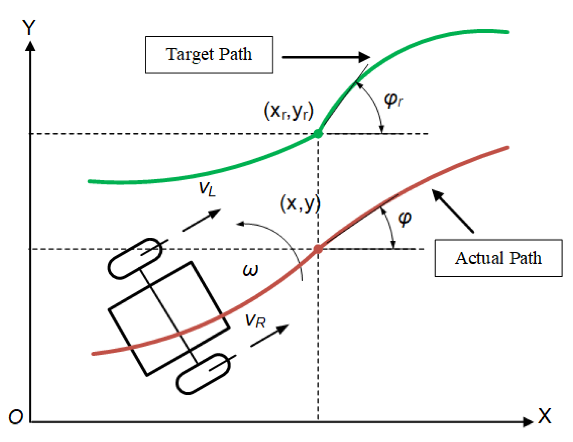
2.1. Mobile Robot Control System

The kinematic model of two wheels mobile robot are shown in Figure 1. According to the relationship between robot velocity v and two driving wheels velocity ( v L , v R ), the robot velocity and angle velocity are expressed as: v = ( v L + v R ) / 2 , ω = ( v L - v R ) / l f , respectively. l f denotes the distance of two wheels. The kinematic model formulation of mobile robot is expressed as,
X ˙ = x ˙ y ˙ θ ˙ = v cos θ v sin θ ω = cos θ 0 sin θ 0 0 1 u
where ( x , y ) is the mobile robot position in Cartesian space and θ is the orientation; u = ( v , ω ) T is the control input and X is the state vector. From the formulation in (1), we can obtain a kinematic model of the reference trajectory by state vector X r = ( x r , y r , θ r ) T and control input u r = ( v r , ω r ) T and it is expressed as:
X ˙ r = x ˙ r y ˙ r θ ˙ r = v r cos θ r v r sin θ r ω r = cos θ r 0 sin θ r 0 0 1 u r
Therefore, we can get the robotic kinematic errors,
X e = cos θ sin θ 0 - sin θ cos θ 0 0 0 1 x r x y r y θ r θ
where X e = [ x e , y e , θ e ] T . The derivative of X ˙ e can be obtained from the error state in (3),
x ˙ e = ω y e v + v r cos θ e y ˙ e = ω x e + v r sin θ e θ ˙ e = ω r ω
The control inputs are reformulated as:
u e = u 1 u 2 = v r cos θ e v ω r ω
Substituting (5) into (4), the kinematic model of X e can be rewritten as
X ˙ e = x ˙ e y ˙ e θ ˙ e = 0 ω 0 ω 0 0 0 0 0 x e y e θ e + u 1 v r sin θ e u 2
The formulation in (6) can be reformulated as the following equation:
X ¯ ˙ e = 0 ω r 0 ω r 0 v r 0 0 0 X ¯ e + 1 0 0 0 0 1 u e
Therefore, the motion control problem of the mobile robot in (1) is converted into a stabilization problem of a nonlinear affine system in (7).

2.2. Nonlinear Model Predictive Control

The NMPC can be converted into a closed-loop optimal control problem in a finite time-horizon, which is subject to the input vector and state vector constraints. The NMPC formulation can be presented as
X j + 1 = ψ 1 X ( j ) + ψ 2 X ( j ) u ( j )
the input and state vector constraints are defined as:
X ( j ) R X , j = 1 , 2 , , N u ( j ) R U , j = 1 , 2 , . . . N u
where X and u denote state vector and input vector, respectively. In a nonlinear affine system (8), ψ 1 ( . ) and ψ 2 ( . ) denote the nonlinear continuous functions. The initial conditions satisfy ψ 1 ( 0 ) = 0 , and N 1 and 1 N N u that denotes the prediction horizon.
In each sampling period, the optimal input vector can be obtained by a given cost function online optimization, thus the NMPC scheme is formulated by iterative solution of optimal control problems. The cost function can be described as the following form function:
S ( X , u ) = i = j j + N 1 L 1 X ( i ) , u ( i ) + L 2 X ( j + N )
where L 1 ( X , u ) denotes the immediate cost and the satisfying condition is L 1 ( 0 , 0 ) = 0 . The cost function S ( X , u ) can be defined as a quadratic form as follows:
S ( j ) = i = 1 N X j + i | j Q 2 + i = 0 N u 1 u j + i | j R 2
where X ( j + i | j ) is the predicted future horizon state; u ( j + i | j ) = u ( j + i | j ) u ( j 1 + i | j ) which is the increment of the input vector; the parameters R and Q represent the constant design weight matrix; the symbol · represents the Euclidean norm of the corresponding vector. The Equation (8) can be reformulated as:
X e j + 1 = ψ 1 X e ( j ) + ψ 2 X e ( j ) u e ( j )
subject   to u u e ( j ) u +
u u ( j ) u +
X X e ( j ) X +
ψ 1 X e = x 1 x 2 x 3 + T ω r x 2 ω r x 1 + v r x 3 0
ψ 2 X e = T 1 0 0 0 0 1
where X e = x 1 , x 2 , x 3 T = x e , y e , θ e T is the state vector, and T is the sampling period; u e = u 1 , u 2 T , u 1 = v r c o s ( θ e ) v , u 2 = ω r ω is the input vector; ( u , u + ) are the upper and lower limits of input variable, and ( u , u + ) , ( x , x + ) are also the upper and lower limits of the input increment variable and state variable, respectively.
To construct the QP problem for online optimization, we introduce the vectors as:
X ¯ = X e ( j + 1 | j ) , . . . , X e ( j + N | j ) T
u ¯ ( j ) = u e ( j | j ) , . . . , u e ( j + N u 1 | j ) T
According to (11), and (15)–(17), we can get the predicted output,
X ¯ ( j ) = H u ¯ ( j ) + ν 1 ^ + ν 2 ^
H = ν 2 X e ( j | j 1 ) 0 ν 2 X e ( j + 1 | j 1 ) 0 ν 2 X e ( j + N 1 | j 1 ) ν 2 X e ( j + N 1 | j 1 )
ν 1 ^ = ν 1 X e ( j | j 1 ) ν 1 X e ( j + 1 | j 1 ) ν 1 X e ( j + N 1 | j 1 )
ν 2 ^ = ν 2 X e ( j | j 1 ) u ( k 1 ) ν 2 X e ( j + 1 | j 1 ) u ( j 1 ) ν 2 X e ( j + N 1 | j 1 ) u ( j 1 )
where H R 3 N × 2 N u , ν 1 ^ R 3 N , and ν 2 ^ R 3 N . Then, the optimization problem in (10) can be rewritten,
minimum H u ¯ ( j ) + ν 1 ^ + ν 2 ^ Q 2 + u ( j ) R 2
subject   to u ¯ u ¯ ( j + 1 ) u ¯ +
u ¯ u ¯ ( j 1 ) u ¯ +
u ¯ u ¯ ( j 1 ) + I ^ u ¯ ( j ) u ¯ +
X ν 1 ^ + ν 2 ^ + H u ¯ ( j ) X +
where I ^ = I 0 0 0 I I 0 I I I R 2 N u × 2 N u
The optimization problem in (19)–(23) can be reformulated as a QP problem:
minimum 1 2 u ¯ T M u ¯ + c T u ¯
subject   to E u ¯ r
u ¯ u ¯ u ¯ +
and the parameter details are given,
M = 2 ( H T η 1 H + η 2 ) R 2 N u × 2 N u
c = 2 H T η 1 ( ν 2 ^ + ν 1 ^ ) R 2 N u
E = I ^ I ^ H H R ( 4 N u + 6 N ) × 2 N u , r = u + u ( j 1 ) u + u ( j 1 ) X + ν 1 ^ + ν 2 ^ X + ν 1 ^ ν 2 ^ R 4 N u + 6 N

3. Varying-Parameter Convergent Differential Neural Network (VPCDNN)

Firstly, we can rewrite the QP problem as follows:
minimum 1 2 d T M d + c T d
subject   to E d r
ζ d ζ +
where d = u ¯ , ζ = u ¯ , ζ + = u ¯ + , and d [ ζ , ζ + ] .
In order to find the optimal solution of the time-varying convex quadratic programming problem, we design the Lagrange function for Equations (27)–(29) as follows:
L d , y = d T M d 2 + c T d + y T E d r
where variable y is the Lagrange-multiplier. From the Lagrangian theorem in Reference [29], if the derivatives of L d , L y are continuous, we give the following algebraic equations of the Lagrange necessary condition by setting the partial derivatives of L ( d , y ) to zero,
L d = M d + c + E T y = 0 L y = E d r = 0
We can rewrite the equation in (31) as the matrix form,
W p = l
W = M E T E 0 R 6 N u + 6 N × 6 N u + 6 N p = d y R 6 N u + 6 N , l = c r R 6 N u + 6 N
where W is a square matrix and invertible; p denotes the vector that needs to be solved by physical limits. It should be noted that the vectors c and r are time-varying parameters. Therefore, the time-varying solver is considered to solve the time-varying QP problem in (27)–(29).
Actually, the optimal solution is under the condition that the equation in (32) is equivalent to zero. So, the error expression is defined as
e ( t ) = W p ( t ) l ( t )
where the error e ( t ) R 6 N u + 6 N and we hope the variable e is close to zero. Therefore, the varying-parameter convergent differential neural network is proposed for the problem in (33),
e ˙ ( t ) = λ exp ( κ t ) P Ω ( e ( t ) )
P Ω e ( t ) = e i , if e i < e i e i , if e i e i e i + , i 1 , , 6 N u + 6 N e i + , if e i > e i +
where the parameters λ and κ are positive constants, which are used to scale the convergence rate; the symbol P Ω ( · ) is the active function. Then, substituting (33) into (34), the differential equation of the solver for the QP problem can be concluded as
W p ˙ ( t ) = W ˙ p ( t ) λ exp ( κ t ) P Ω ( W p ( t ) l ( t ) ) + l ˙ ( t )
The block diagram of the VPCDNN model (35) is shown in Figure 2. Finally, for the online solving process, the neural network consists of N p neurons and the neural network is constructed as
p ˙ i = j = 1 N p w ˙ i j p i + j = 1 N p ρ i j w i j p ˙ i λ exp ( κ t ) P Ω j = 1 N p w i j p i l i + l ˙ i
where p i , p ˙ i , l i , l ˙ i are the i-th elements of variable p, p ˙ , l i , l ˙ i , respectively; w i j , w ˙ i j , η i j , η ˙ i j are the i-th row and j-th column elements of variable W, I, respectively. Figure 3 exhibits the detailed structure of the VPCDNN model.

4. Convergence and Robustness Analysis of VPCDNN

4.1. Convergence Analysis

It should be noted that the VPCDNN algorithm is a special type of Hopfield-neural network because the network fits the Hopfield-neural network structure with reference to the differential equation theory.
If there exists the optimal solution d for (27)–(29), the vector p converges to equilibrium point p from all initial states p ( 0 ) , which means the VPCDNN can achieve the convergence and the stable point p of VPCDNN is the optimal solution of the QP problem. Firstly, we design the Lyapunov function of error variable e ( t ) and then find the minimum point of the Lyapunov function. The detailed proof of convergence is given as follows.
Theorem 1.
For the time-varying QP problem in (27)–(29), assume that there is the optimal solution d for the QP problem when the monotone nondecreasing activation function of P Ω acts on the error variable. From any initial state p ( 0 ) R 6 N u + 6 N , the state vector p ( t ) = [ d T ( t ) , y T ( t ) ] T of VPCDNN globally converges to equilibrium point p ( t ) = d T ( t ) , y T ( t ) T , where the first n-elements of p ( x ) are the optimal solution of (27)–(29).
Proof. 
Considering the candidate Lyapunov function as
F ( t ) = 1 2 e T ( t ) e ( t ) , e ( t ) 0
It is obvious that the Lyapunov function in (37) is a positive function. The time derivative of F ( t ) can be obtained as
F ˙ ( t ) = d F ( t ) d t = e T ( t ) e ˙ ( t )
Then, substituting (34) into (38), we obtain
F ˙ ( t ) = λ exp ( κ t ) e T ( t ) P Ω e ( t ) = λ exp ( κ t ) i = 1 N p e i ( t ) P Ω e i ( t )
where e i ( t ) represents the ith element of variable e ( t ) ; P Ω e ( t ) is the ith projection element of variable P Ω e ( t ) . Since P Ω e ( t ) is the monotone nondecreasing projection function, it is easy to obtain
e i ( t ) P Ω e i ( t ) = > 0 , if e i ( t ) 0 = 0 , if e i ( t ) = 0
Therefore, we can obtain the following,
F ˙ ( t ) = > 0 , if e i ( t ) 0 = 0 , if e i ( t ) = 0
According to the (41), we know that if and only if e i ( t ) = 0 , F ˙ ( t ) is equal to zero. Therefore, p ( t ) p ( t ) globally converges to 0 based on Lyapunov theory [30], which also means d ( t ) d ( t ) globally converges to zero. So, the proof of VPCDNN is finished. □

4.2. Robustness Analysis

Considering the disturbance model in (35) as follows,
W p ˙ ( t ) = ( W ˙ + B ( t ) ) p ( t ) λ exp ( κ t ) P ( W p ( t ) l ( t ) ) + l ˙ ( t ) + ξ ( t )
where B R 6 N u + 6 N × 6 N u + 6 N is the disturbing term of W; ξ R n + m is the error from the VPCDNN model.
Theorem 2.
If B ( t ) μ B , ξ ( t ) μ ξ , W 1 μ W , l ( t ) μ l , and μ B , where μ ξ , μ W , μ l are all positive parameters, the error e ( t ) will converge to 0 under the condition of λ a exp ( κ t ) μ B μ A > 0 .
Proof. 
Substituting the (33), (34) into (42), we can conclude
e ˙ ( t ) = λ exp ( κ t ) P Ω e ( t ) B ( t ) W 1 e ( t ) + ξ ( t ) B ( t ) W 1 l ( t )
We choose a Lyapunov function as
V ( t ) = 1 2 e T ( t ) e ( t ) = 1 2 j = 1 6 N u + 6 N e i 2 ( t )
where V ( t ) is the non-negative variable.
Then, we can obtain the time derivative of V ( t ) ,
V ( t ) = e T ( t ) e ˙ ( t ) = e T ( t ) ( λ exp ( κ t ) P Ω ( e ( t ) ) B ( t ) W 1 e ( t ) + ξ ( t ) B ( t ) W 1 l ( t ) ) = λ exp ( κ t ) e T ( t ) P Ω ( e ( t ) ) + e T ( t ) ψ ( t ) e ( t ) + e T ( t ) ξ ( t ) + e T ( t ) B ( t ) W 1 l ( t ) = λ exp ( κ t ) e T ( t ) P Ω ( e ( t ) ) + e T ( t ) ψ ( t ) + ψ T ( t ) 2 e ( t ) + e T ( t ) ξ ( t ) + e T ( t ) B ( t ) W 1 l ( t )
where ψ ( t ) = B ( t ) W 1 . Moreover,
e T ( t ) ψ ( t ) + ψ T ( t ) 2 e ( t ) e T ( t ) e ( t ) λ max ψ ( t ) + ψ T ( t ) 2 e T ( t ) e ( t ) B ( t ) W 1 ( t ) e T ( t ) e ( t ) μ B μ W
e T ( t ) ξ ( t ) i = 1 6 N u + 6 N e i μ ξ
e T ( t ) B ( t ) W 1 l ( t ) i = 1 6 N u + 6 N e i · B ( t ) W 1 l ( t ) i = 1 6 N u + 6 N e i μ B μ ξ μ l
Therefore, substituting (46)–(47) into (45),
V ˙ ( t ) λ exp ( κ t ) e T ( t ) P Ω e ( t ) + e T ( t ) e ( t ) μ B μ W + i = 1 6 N u + 6 N e i μ ξ + i = 1 6 N u + 6 N e i μ B μ ξ μ l = i = 1 6 N u + 6 N e i λ exp ( κ t ) P Ω ( e i ) μ B μ W e i μ ξ μ B μ ξ μ l
We define the Θ 1 = λ exp ( κ t ) P Ω ( e i ) μ B μ W e i μ ξ μ B μ ξ μ l . We know variable Θ 1 may be positive or negative.
  • if Θ 1 0 , so V ˙ 0 . It is obvious that the error variable e ( t ) converges to zero from the Lyapunov theorem and the state variable p converges to the optimal solution p .
  • if Θ 1 < 0 , then V ˙ < δ ( δ > 0 ) . Therefore, V ˙ may be positive or negative.
    (a)
    if V ˙ 0 , we know the error variable e ( t ) converges to zero, also the state variable p will converge to optimal solution p .
    (b)
    if V ˙ > 0 ( 0 < V ˙ < δ ) , and consider the linear activation function Θ 1 ( e ( t ) ) = a e ( t ) ( a 1 ) , and λ a exp ( κ t ) μ B μ W > 0 , so we can obtain,
    V ˙ i = 1 6 N u + 6 N e i ( λ exp ( κ t ) a e i μ B μ W e i μ ξ μ B μ W μ l ) ) = λ a exp ( κ t ) μ B μ W i = 1 n + m e i e i μ ξ + μ B μ W μ l λ a exp ( κ t ) μ B μ W
It is easy to obtain λ > μ B μ W a . According to (50), in this case, 0 < V ˙ < δ , so V ( t ) increase that means e i will increase, and V ˙ will decrease. Therefore, V ˙ always exists a moment V ˙ 0 , then the control system will stabilize again.
It should be noted that when v ˙ ( t ) = 0 , e i = e + , e + is the upper bound. We define Θ 2 = μ ξ + μ B μ W μ l λ a exp ( κ t ) μ B μ W . If V ˙ ( t ) = 0 , i = 1 6 N u + 6 N e i e i Θ 2 = 0 and the variable e i can be seen as the input, the function e i e i Θ 2 will obtain the minimum output, if e i = 0.5 Θ 2 . Moreover, e i e i Θ 2 > 0 when e i > Θ 2
We know i = 1 6 N u + 6 N e i e i Θ 2 = 0 and the function mentioned above has a negative minimum output. We assume that e j ( i = j ) is the upper bound e + , so e j will be achieved if and only if the rest 6 N u + 6 N 1 terms e i e i Θ 2 obtain the minimum point. Therefore,
i = 1 6 N u + 6 N e i e i Θ 2 = i = 1 , i j 6 N u + 6 N e i e i Θ 2 + e j e j Θ 2
Then, Θ 2 = μ ξ + μ B μ W μ l λ a exp ( κ t ) μ B μ W is substituted in (51) and obtain
i = 1 6 N u + 6 N e i e i Θ 2 = e j 2 e j μ ξ + μ B μ W μ l λ a exp ( κ t ) μ B μ W 6 N u + 6 N 1 4 μ ξ + μ B μ W μ l λ a exp ( κ t ) μ B μ W 2 = 0
According to analysis, we can conclude the upper bound e j ,
e j = 1 2 ( 1 + 6 N u + 6 N ) η
where η = μ ξ + μ B μ W μ l λ a exp ( κ t ) μ B μ W , e e n d ( e n d = 6 N u + 6 N ) converge to zero. □

5. Simulation

In this section, the proposed VPCDNN algorithm is tested with a two-wheel mobile robot in simulation. Two type trajectories will be tested for tracking: circle-shape trajectory (the linear velocity v and angular velocity w are time constant); ’8’-shape trajectory (the linear velocity v and angular velocity w are time varying) and the trajectory function in Cartesian space will be given in Section 5.2. Both of the two trajectories will be tested in mobile robot tracking and the detailed analysis of the simulation results will be given in Section 5.1 and Section 5.2.

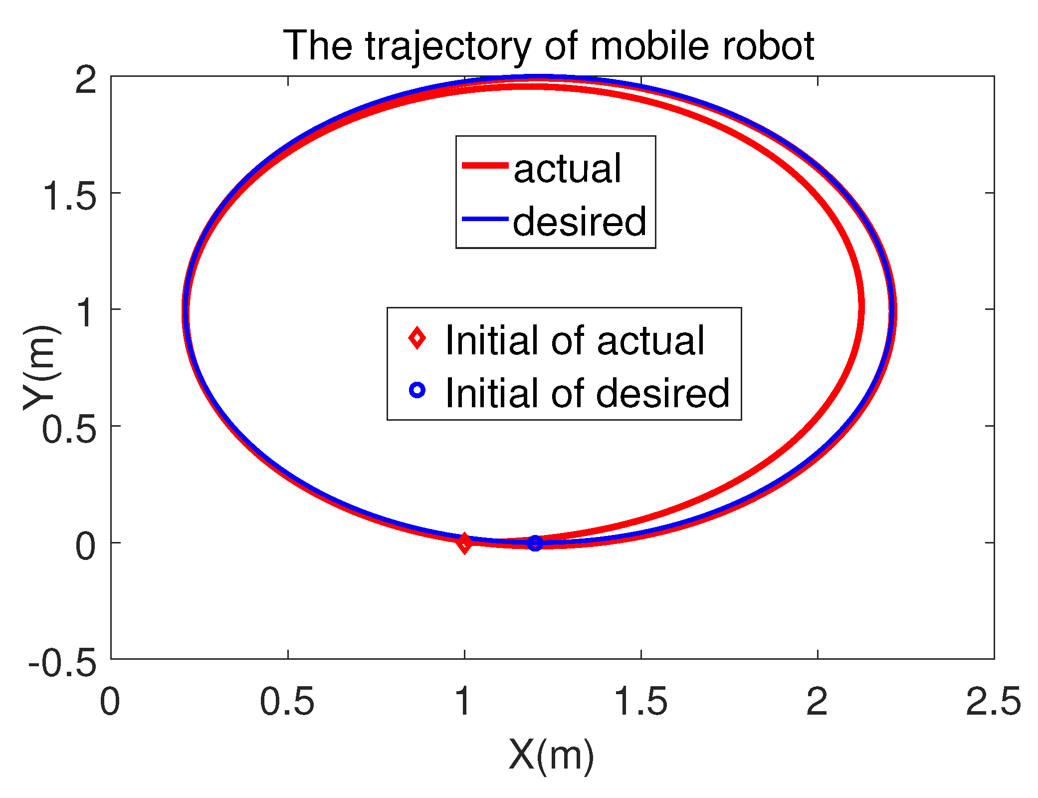
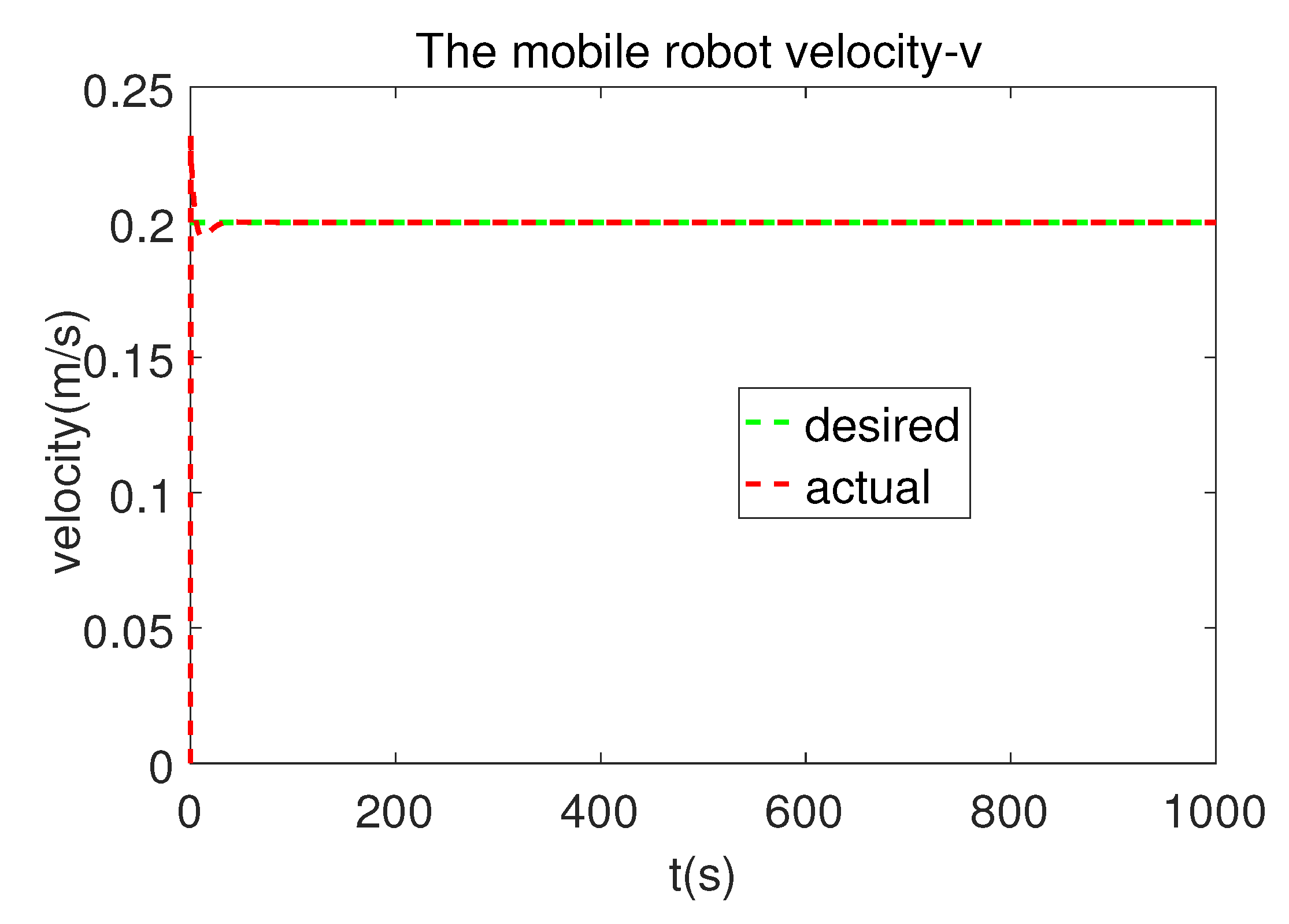
5.1. Circle-Shape Tracking

In this part, we control the mobile robot to track the circle-shape trajectory, where the reference linear velocity v and angular velocities ω are set as v = 0.2 m/s, w = 0.2 rad/s, respectively. In order to prove the tracking performance of our method, the initial position of the mobile robot is set as X r ( 0 ) = [ 1.0 ; 0 ; 0 ] which does not coincide with the reference initial point X ( 0 ) = [ 1.2 ; 0 ; 0 ] .
The parameters of nonlinear MPC are listed as: N = 3 , N u = 2 , η 1 = 3 I , η 2 = I . The neural network parameter λ and κ are set as: λ = 0.1 , κ = 1 e 4 . The sampling period of MPC is t = 0.1 s .
From Figure 4 and Figure 5, it can be seen that the trajectories of the mobile robot quickly converge to the reference trajectory, regardless of the initial position of the mobile robot. From Figure 6 and Figure 7, we can see the mobile robot’s linear and angular velocity are extremely close to the reference values. We can also see that the tracking errors of the mobile robot quickly converge to zero as shown in Figure 8 and Figure 9.

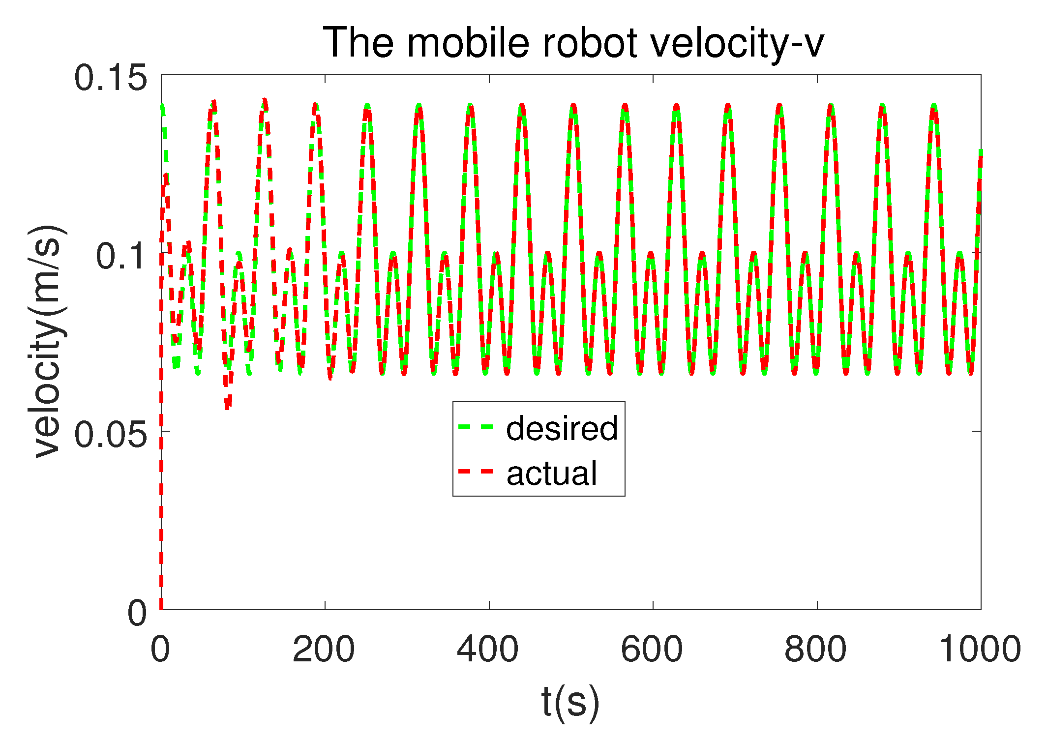
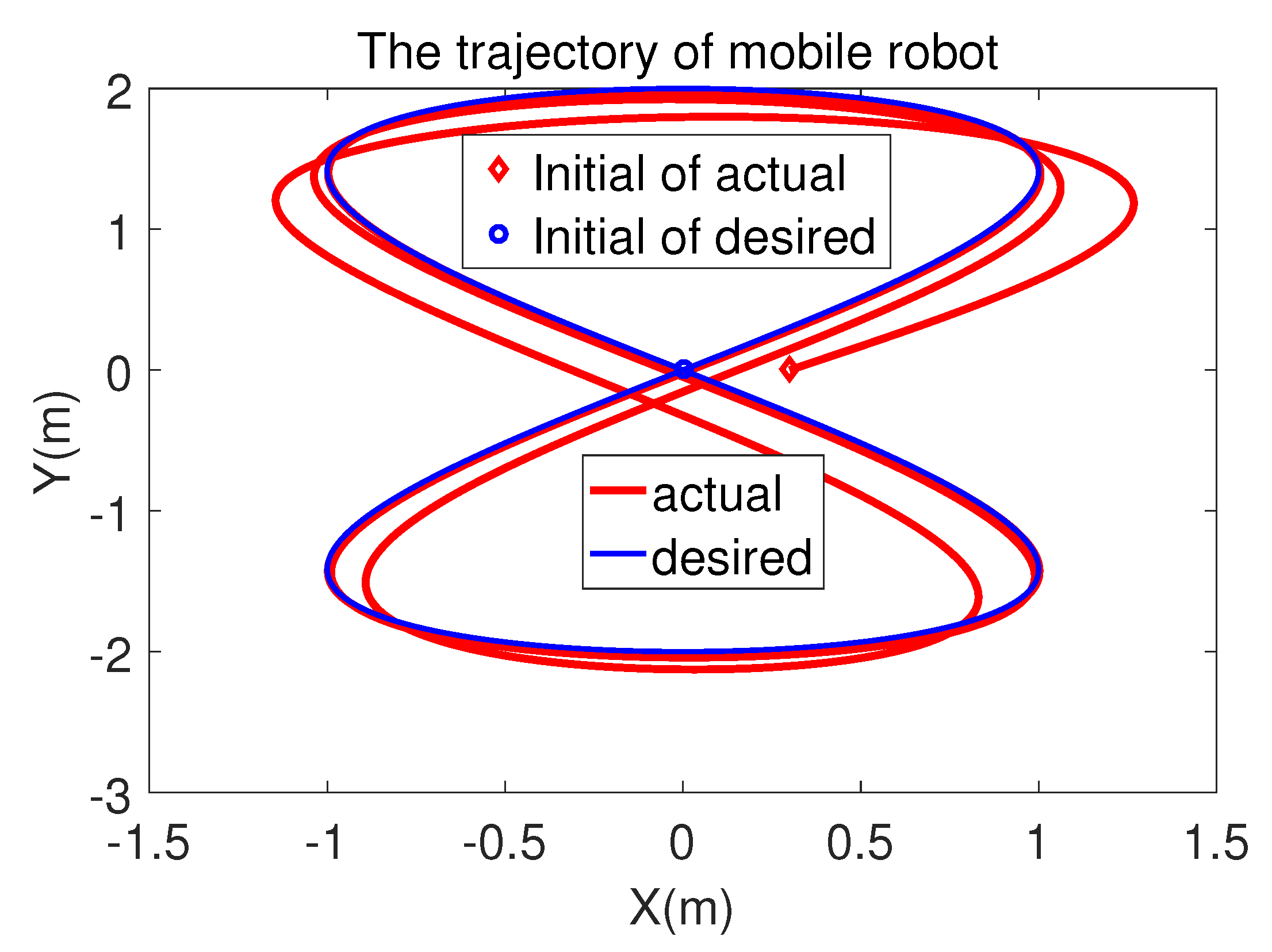
5.2. ‘8’-Shape Tracking

The mobile robot’s task in this scenario is to track the ‘8’-shape trajectory for the periodic movement with changing linear and angular velocity, starting from initialized positions and orientations. The reference trajectory of ‘8’-shape is given as
x = s i n ( 0.1 t ) y = 2 s i n ( 0.05 t )
The parameters of nonlinear MPC are listed as: N = 3 , N u = 2 , η 1 = 3 I , η 2 = I . The convergence parameter λ and κ are set as: λ = 0.1 , κ = 1 e 4 . The sampling period of MPC is set t = 0.1 s.
The initial position of the reference trajectory is X r ( 0 ) = [ 0 ; 0 ; 0.7854 ] , and the initial position of the mobile robot is X ( 0 ) = [ 0.3 ; 0 ; 0.7 ] . From Figure 10 and Figure 11, we can see that the trajectories of the mobile robot quickly converge to the reference trajectory even changing the linear and angular velocity of the robot periodically. From Figure 12 and Figure 13, we can see that the mobile robot’s linear and angular velocity follow the reference velocity quite well. Figure 14 and Figure 15 show that the tracking errors of the mobile robot quickly converge to zero.
In both scenarios, the mobile robot is able to track the reference trajectory successfully. The convergence rate is very fast which is very important for running in real time. The mobile robot solves the trajectory tracking task with the optimal solution from different initialized positions and orientations. The tracking errors also converge very fast to zero. These results show the robustness and effectiveness of the proposed method. Moreover, the overall success rate, fast convergence, and the performance of the proposed VPCDNN based MPC method indicates its strong ability in real time.
In order to verify the effectiveness of VPCDNN, we have added contrast tests using LNN methods which include the time- invariant method called the recurrent neural network (gradient-descent based) in Reference [31]. The comparison results are shown in Figure 16, Figure 17 and Figure 18. We can conclude that both VPCDNN and RNN can track the given trajectory, but VPCDNN has the faster convergence speed which is better for the time-varying optimization problem.
In addition, in this paper, we connect CarSim software to a Matlab/Simulink model and test the VPCDNN-MPC method to track the sinusoidal trajectory which is shown in Figure 19. The requirements of simulator platform were Matlab2018b/Simulink, Carsim2016, Windows10.

6. Conclusions

In this paper, the MPC scheme is presented to the control problem over finite time-horizon with the input and state vector of a mobile robot. In the reformation of the nonlinear affine system of a mobile robot, the nonlinear non-convex optimization problem is converted to the nonlinear convex optimization problem. Therefore, the new network of VPCDNN is also presented to solve the online optimization QP problem of NMPC. In order to test the proposed method, the mobile robot tracks the circle-shape and ’8’-shape trajectories in simulation. The results show that the proposed method successfully tracked the desired trajectories. The method converges quickly to the solution with the VPCDNN. The tracking errors of the VPCDNN based NMPC are maintained at a very low level. All these characteristics enable our proposed method to be a powerful and efficient solution to the control problem of mobile robots.

Author Contributions

Conceptualization, Y.H. and G.C.; methodology, Y.H. and H.S.; software Y.H. and S.M.; validation, L.Z. and H.S.; formal analysis, S.M. and H.S.; investigation, data curation, L.Z.; writing-original draft preparation, Y.H.; writing-reviewand editing, G.C. and H.S.; supervision, A.K. and G.C.; project administration, A.K.

Funding

This work was supported by the German Research Foundation (DFG) and the Technical University of Munich (TUM) in the framework of the Open Access Publishing Program. This research also received funding from the European Union’s Horizon 2020 Framework Programme for Research and Innovation under the Specific Grant Agreement No. 785907 (Human Brain Project SGA2).

Conflicts of Interest

The authors declare no conflict of interest. The funders had no role in the design of the study; in the collection, analyses, or interpretation of data; in the writing of the manuscript, or in the decision to publish the results.

Abbreviations

The following abbreviations are used in this manuscript:
NMPCnonlinear model predictive control
VPCDNNvarying-parameter convergent differential neural network
QPquadratic programming
SMCsliding mode control
GPNNgeneral projection neural network
PDNNprimal dual neural network

References

  1. Brockett, R.W. Asymptotic stability andfeedback stabilization. Differ. Geom. Control Theory 1983, 27, 181–208. [Google Scholar]
  2. Al-Araji, A.S. Development of kinematic path-tracking controller design for real mobile robot via back-stepping slice genetic robust algorithm technique. Arab. J. Sci. Eng. 2014, 39, 8825–8835. [Google Scholar] [CrossRef]
  3. Fukushima, H.; Muro, K.; Matsuno, F. Sliding-mode control for transformation to an inverted pendulum mode of a mobile robot with wheel-arms. IEEE Trans. Ind. Electron. 2014, 62, 4257–4266. [Google Scholar] [CrossRef]
  4. Ostafew, C.J.; Schoellig, A.P.; Barfoot, T.D. Visual teach and repeat, repeat, repeat: Iterative learning control to improve mobile robot path tracking in challenging outdoor environments. In Proceedings of the 2013 IEEE/RSJ International Conference on Intelligent Robots and Systems, Tokyo, Japan, 3–7 November 2013; pp. 176–181. [Google Scholar]
  5. Li, T.H.; Chang, S.J.; Tong, W. Fuzzy target tracking control of autonomous mobile robots by using infrared sensors. IEEE Trans. Fuzzy Syst. 2004, 12, 491–501. [Google Scholar] [CrossRef]
  6. Khalaji, A.K.; Moosavian, S.A.A. Robust adaptive controller for a tractor–trailer mobile robot. IEEE/ASME Trans. Mechatron. 2013, 19, 943–953. [Google Scholar] [CrossRef]
  7. Park, B.S.; Yoo, S.J.; Park, J.B.; Choi, Y.H. A simple adaptive control approach for trajectory tracking of electrically driven nonholonomic mobile robots. IEEE Trans. Control Syst. Technol. 2010, 18, 1199–1206. [Google Scholar] [CrossRef]
  8. Armesto, L.; Girbés, V.; Sala, A.; Zima, M.; Šmídl, V. Duality-based nonlinear quadratic control: Application to mobile robot trajectory-following. IEEE Trans. Control Syst. Technol. 2015, 23, 1494–1504. [Google Scholar] [CrossRef]
  9. Hendzel, Z.; Penar, P. Optimal Control of a Wheeled Robot. In Conference on Automation; Springer: Cham, Switzerland, 2019; pp. 473–481. [Google Scholar]
  10. Patrinos, P.; Bemporad, A. An accelerated dual gradient-projection algorithm for embedded linear model predictive control. IEEE Trans. Autom. Control. 2013, 59, 18–33. [Google Scholar] [CrossRef]
  11. Frison, G.; Sørensen, H.H.B.S.; Dammann, B.; Jørgensen, J.B.J. High-performance small-scale solvers for linear model predictive control. In Proceedings of the 2014 European Control Conference (ECC), Strasbourg, France, 24–27 June 2014; pp. 128–133. [Google Scholar]
  12. Nascimento, T.P.; Dórea, C.E.T.; Goncalves, L.M.G. Nonholonomic mobile robots’ trajectory tracking model predictive control: A survey. Robotica 2018, 36, 676–696. [Google Scholar] [CrossRef]
  13. Nascimento, T.P.; Moreira, A.P.; Conceição, A.G.S. Multi-robot nonlinear model predictive formation control: Moving target and target absence. Robot. Auton. Syst. 2013, 61, 1502–1515. [Google Scholar] [CrossRef]
  14. Vajedi, M.; Azad, N.L. Ecological adaptive cruise controller for plug-in hybrid electric vehicles using nonlinear model predictive control. IEEE Trans. Intell. Transp. Syst. 2015, 17, 113–122. [Google Scholar] [CrossRef]
  15. Lima, P.U.; Ahmad, A.; Dias, A.; Conceição, A.G.; Moreira, A.P.; Silva, E.; Nascimento, T.P. Formation control driven by cooperative object tracking. Robot. Auton. Syst. 2015, 63, 68–79. [Google Scholar] [CrossRef]
  16. Nascimento, T.P.; Dórea, C.E.T.; Goncalves, L.M.G. Nonlinear model predictive control for trajectory tracking of nonholonomic mobile robots: A modified approach. Int. J. Adv. Robot. Syst. 2018, 15, 1729881418760461. [Google Scholar] [CrossRef]
  17. Mesbah, A. Stochastic model predictive control: An overview and perspectives for future research. IEEE Control Syst. Mag. 2016, 36, 30–44. [Google Scholar]
  18. Nascimento, T.P.; Basso, G.F.; Dorea, C.; Goncalves, L.M.G. Perception-driven Motion Control Based on Stochastic Nonlinear Model Predictive Controllers. IEEE/ASME Trans. Mechatron. 2019, 1, 1–11. [Google Scholar] [CrossRef]
  19. Rubagotti, M.; Patrinos, P.; Bemporad, A. Stabilizing linear model predictive control under inexact numerical optimization. IEEE Trans. Autom. Control 2014, 59, 1660–1666. [Google Scholar] [CrossRef]
  20. Park, H.; Sun, J.; Pekarek, S.; Stone, P.; Opila, D.; Meyer, R.; DeCarlo, R. Real-time model predictive control for shipboard power management using the IPA-SQP approach. IEEE Trans. Control Syst. Technol. 2015, 23, 2129–2143. [Google Scholar] [CrossRef]
  21. Sekiguchi, S.; Yorozu, A.; Kuno, K.; Okada, M.; Watanabe, Y.; Takahashi, M. Nonlinear model predictive control for two-wheeled service robots. In International Conference on Intelligent Autonomous Systems; Springer: Cham, Switzerland, 2018; pp. 452–463. [Google Scholar]
  22. Pan, Y.; Wang, J. Model predictive control of unknown nonlinear dynamical systems based on recurrent neural networks. IEEE Trans. Ind. Electron. 2012, 59, 3089–3101. [Google Scholar] [CrossRef]
  23. Li, Z.; Xiao, H.; Yang, C.; Zhao, Y. Model predictive control of nonholonomic chained systems using general projection neural networks optimization. IEEE Trans. Syst. Man Cybern. Syst. 2015, 45, 1313–1321. [Google Scholar] [CrossRef]
  24. Xiao, H.; Li, Z.; Chen, C.P. Formation control of leader-follower mobile robots’ systems using model predictive control based on neural-dynamic optimization. IEEE Trans. Ind. Electron. 2016, 63, 5752–5762. [Google Scholar] [CrossRef]
  25. Ke, F.; Li, Z.; Yang, C. Robust Tube-Based Predictive Control for Visual Servoing of Constrained Differential-Drive Mobile Robots. IEEE Trans. Ind. Electron. 2018, 65, 3437–3446. [Google Scholar] [CrossRef]
  26. Li, Z.; Yuan, Y.; Ke, F.; He, W.; Su, C. Robust Vision-Based Tube Model Predictive Control of Multiple Mobile Robots for Leader-Follower Formation. IEEE Trans. Ind. Electron. 2019, in press. [Google Scholar] [CrossRef]
  27. Zhang, Y.; Wang, J. A dual neural network for convex quadratic programming subject to linear equality and inequality constraints. Phys. Lett. A 2002, 298, 271–278. [Google Scholar] [CrossRef]
  28. Hu, Y.; Li, Z.; Li, G.; Yuan, P.; Yang, C.; Song, R. Development of sensory-motor fusion-based manipulation and grasping control for a robotic hand-eye system. IEEE Trans. Syst. Man Cybern. Syst. 2017, 7, 1169–1180. [Google Scholar] [CrossRef]
  29. Boyd, S.; Vandenberghe, L. Convex Optimization; Cambridge University Press: Cambridge, UK, 2004. [Google Scholar]
  30. Coddington, E.A.; Levinson, N.; Teichmann, T. Theory of ordinary differential equations. Phys. Today 1956. [Google Scholar] [CrossRef]
  31. Xia, Y.; Wang, J.; Fok, L.M. Grasping-force optimization for multifingered robotic hands using a recurrent neural network. IEEE Trans. Robot. Autom. 2004, 20, 549–554. [Google Scholar] [CrossRef]
Figure 1. Kinematic model of two-wheels mobile robot.
Robotics 08 00064 g001
Figure 2. The block diagram of VPCDNN model.
Robotics 08 00064 g002
Figure 3. Structure of VPCDNN model.
Robotics 08 00064 g003
Figure 4. Tracking result of circle-shape trajectory.
Robotics 08 00064 g004
Figure 5. Tracking result of orientation angle.
Robotics 08 00064 g005
Figure 6. Linear velocity of mobile robot.
Robotics 08 00064 g006
Figure 7. Angular velocity of mobile robot.
Robotics 08 00064 g007
Figure 8. Tracking error in Cartesian space.
Robotics 08 00064 g008
Figure 9. Tracking error of orientation angle.
Robotics 08 00064 g009
Figure 10. Tracking result of ‘8’-shape trajectory.
Robotics 08 00064 g010
Figure 11. Tracking result of orientation angle.
Robotics 08 00064 g011
Figure 12. Linear velocity of mobile robot.
Robotics 08 00064 g012
Figure 13. Angular velocity of mobile robot.
Robotics 08 00064 g013
Figure 14. Tracking error in Cartesian space.
Robotics 08 00064 g014
Figure 15. Tracking error of orientation angle.
Robotics 08 00064 g015
Figure 16. Comparison results of ‘8’-shape using LNN.
Robotics 08 00064 g016
Figure 17. Comparison results of X e , Y e error using LNN.
Robotics 08 00064 g017
Figure 18. Comparison results of θ e error using LNN.
Robotics 08 00064 g018
Figure 19. Tracking the sinusoidal trajectory using vehicle in Carsim simulation.
Robotics 08 00064 g019

