Article

Real-Time 3D Map Building in a Mobile Robot System with Low-Bandwidth Communication

Department of Intelligent Robotics, Toyama Prefectural University, 5180 Kurokawa Imizu, Toyama 939-0398, Japan
*
Author to whom correspondence should be addressed.
Robotics 2023, 12(6), 157; https://doi.org/10.3390/robotics12060157
Submission received: 20 October 2023 / Revised: 17 November 2023 / Accepted: 20 November 2023 / Published: 22 November 2023
(This article belongs to the Special Issue Active Methods in Autonomous Navigation)

Abstract

:
This paper presents a new 3D map building technique using a combination of 2D SLAM and 3D objects that can be implemented on relatively low-cost hardware in real-time. Recently, 3D visualization of the real world became increasingly important. In robotics, it is not only required for intelligent control, but also necessary for operators to provide intuitive visualization. SLAM is generally applied for this purpose, as it is considered a basic ability for truly autonomous robots. However, due to the increase in the amount of data, real-time processing is becoming a challenge. Therefore, in order to address this problem, we combine 2D data and 3D objects to create a new 3D map. The combination is simple yet robust based on rotation, translation, and clustering techniques. The proposed method was applied to a mobile robot system for indoor observation. The results show that real-time performance can be achieved by the system. Furthermore, we also combine high and low-bandwidth networks to deal with network problems that usually occur in wireless communication. Thus, robust wireless communication can be established, as it ensures that the missions can be continued even if the system loses the main network.

1. Introduction

Representing the real world in 3D visualization became increasingly important. In robotics, 3D maps unlock smarter capabilities for the robots [1]; for example, environmental exploration and localization [2], search and rescue [3], motion planning and automation [4], monitoring [5], and some others. Utilization of 3D maps remains challenging, especially for real-time implementation using mobile devices. Due to limited computing and memory resources, the amount of data brings a significant burden to the onboard processing, which can slow down overall performance [6,7]. On the other hand, missions and data collection have to be continued. Therefore, data compression is required to handle this issue.
In ground exploration missions, mobile robots are one of the most widely used technologies due to their mobility and adaptation to environments. Wheeled [8,9] or crawler robots [10,11] all became essential parts for both domestic and industrial applications. In domestic applications, they are more popular as service robots, for example, cleaning kitchens [12], cleaning floors such as the Roomba, and indoor observation [13]. Meanwhile, for industrial applications, many of them are intended for agriculture [14,15], hazardous tasks, saving human lives, and disaster response [16].
In order to work intelligently, maps are required in robot operations, even more so for autonomous control [17,18]. Simultaneous localization and mapping (SLAM) is generally applied for this purpose. It builds a map of the environment, and at the same time, locates the robot position on the map [19]. In addition, SLAM is also considered a basic ability and is highly encouraged for explorer robots [20,21]. Apart from the reasons above, SLAM can be used to provide an intuitive visualization (i.e., maps) of what the environment looks like [22]. It helps humans better understand the current situation. These are the reasons why the development and applications of SLAM were a major research topic for at least the last decade. SLAM is not only used by the robots, but is also useful for the humans.
In this paper, we focus on how to achieve real-time implementation of 3D map building. We believe that nowadays the development of SLAM and its related matters should be applicable and real-time oriented. There were several techniques related to this concern. In [23], a combination of perpendicular 2D data from two 2D laser scanners is proposed. The observations are accomplished in indoor regions with two mobile robots in parallel. Then, translational and rotational values are applied to the perpendicular data to construct a 3D point cloud map. However, real-time computation cannot be achieved since the combination is achieved offline, which requires around fifteen minutes; similarly as in [24,25], where offline computation is performed. Next, the fusion of a 2D light detection and ranging (LiDAR) and a depth camera [26] or a stereo camera [27] was developed. The cameras are used to improve the accuracy of 2D SLAM. Although additional information was combined, only a 2.2% to 3.6% improvement can be achieved. Furthermore, it also results in increased computational requirements.
Real-time implementation of large amounts of data is challenging, especially for processing requirements. As mentioned previously, one of the solutions is to compress the amount of data. The other solution is, of course, increasing the processing capability. In [2,22], real-time computation of 3D map building can be achieved using mobile robots. They use an Intel Core i7-4790K CPU 32 GB RAM and a Core i7-3555LE CPU 8 GB RAM, respectively. The method requires 1.56 s out of 3 s to update the map with 1.33× of data downsampling [22]. A mobile robot system in [28] performed 3D mapping with high quality and repeatability. It employs a Velodyne Puck LITE 3D laser scanner and an inertial measurement unit (IMU) sensor to run an online SLAM algorithm. However, in the implementation, the mobile robot was steered remotely using a wireless joystick, and the amount of data will be nearly impossible to implement on low-cost hardware to perform real-time observation. Modern SLAM algorithms, such as ORB-SLAMs [29,30,31], may also run in real time on embedded systems [32,33]. Nevertheless, they rely on multithreading, which is also limited in this system.
In real-world situations, degraded communication may occur during missions [2], especially in restricted areas that require kilometers of operating distance [10]. Therefore, to handle this issue, we also combine high and low-bandwidth networks in the system, i.e., Wi-Fi and long-range (LoRa). Wi-Fi, due to its high bandwidth, has a short communication range and is thus easily affected by environments; for example, buildings, trees, tunnels, underground, sea water, and some others. LoRa, on the other hand, has a much longer communication range and is more robust to the environments [34]. Furthermore, LoRa can maintain its communication for several kilometers even in urban areas [35], and its network can be scaled to increase the number of nodes [36]. Similar to [37], which combines Wi-Fi and a radio-frequency (RF) module (200 kbps) for sharing data between two mobile robots and constructing a 3D map, network limitations force the system to compress the data for real-time performance. The difference is that we use a lower communication bandwidth of about 6.01 kbps–22 kbps, which requires further data compression. Furthermore, they still require the high-bandwidth network to construct a full 3D map.
There are two restrictions in the proposed system, i.e., limited onboard computing resources and low-bandwidth communication. Based on the state-of-the-art above, a new technique is required in order to perform real-time 3D map building. Therefore, we propose a new real-time 3D map building technique using the combination of 2D SLAM and 3D objects. The technique is applied and focused on the mobile robot system with Wi-Fi and LoRa as the communication networks, as shown in Figure 1. Wi-Fi is used as the main communication network, with LoRa serving as a backup. Multi-bandwidth networks proved their impact on signal interference, shadowing, and wireless communication attenuation [38,39]. Hence, robust wireless communication can be established.
The contributions of this research can be summarized as follows: (1) The system utilizes low-cost devices, i.e., a Raspberry Pi controller and LoRa devices on the mobile robot, and an entry-level PC controller with an Intel Core i5-10210U CPU 8 GB RAM for controlling and monitoring the mobile robot. (2) We combine high and low-bandwidth networks to establish a robust wireless communication system. All observation data need to be sent wirelessly, creating a new data size restriction, and hence data compression is required. Lastly, (3) lightweight and efficient algorithms must be developed. All developed algorithms have to be simple, can be installed on low-cost hardware, and have real-time capabilities. These introduce the main target of the system, which performs the proposed method in real-time at a refresh rate of at least 1 Hz for both communication bandwidths. A real-time system is essential for operators as it gives direct results about environmental conditions. 3D maps will also increase intuitiveness to better understand the environment. Finally, a fully wireless communication system enables a barrier between the operators and observation fields, which increases safety for some crucial missions, such as search and rescue and disaster response.
The rest of this paper is organized as follows. In Section 2, the system configuration is described. Section 3 explains the proposed approach in detail. Section 4 shows the experimental results with its discussion. Last but not least, Section 5 is the conclusion and future work.

2. System Configuration

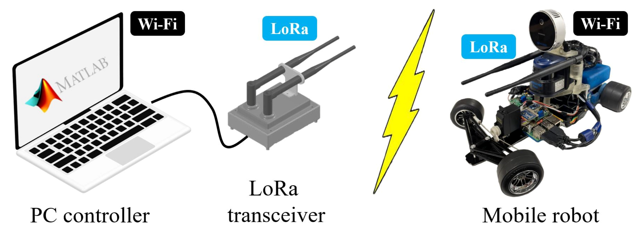
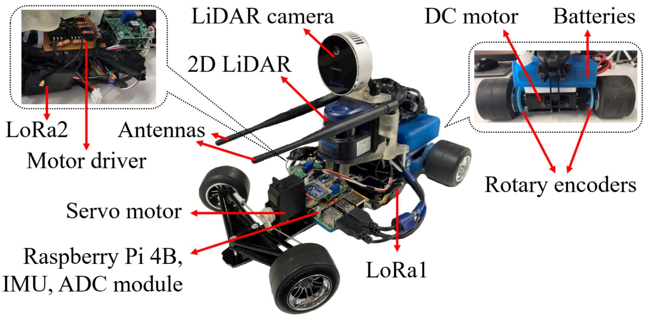
2.1. Hardware Design

In this system, there is a PC controller, a LoRa transceiver, and a mobile robot, as shown in Figure 1. The PC controller is used by an operator to control and monitor the mobile robot. It is also connected to the LoRa transceiver to communicate with the mobile robot through the low-bandwidth communication using LoRa devices. Figure 2 shows several devices installed on the mobile robot. We use a 2D LiDAR and a LiDAR camera as the main sensors to observe the environment. By using both sensors, 2D and 3D data can be provided from the mobile robot.
The hardware specifications are summarized in Table 1. The LoRa transceiver is basically used to convert serial data from LoRa devices to USB signal. Thus, the PC controller can read the serial data and communicate with the mobile robot. The same as in [40], there are two LoRa devices used on the PC controller and the mobile robot to increase the communication bandwidth. This is intended for sending large data, such as 2D and 3D data when using the low-bandwidth communication.

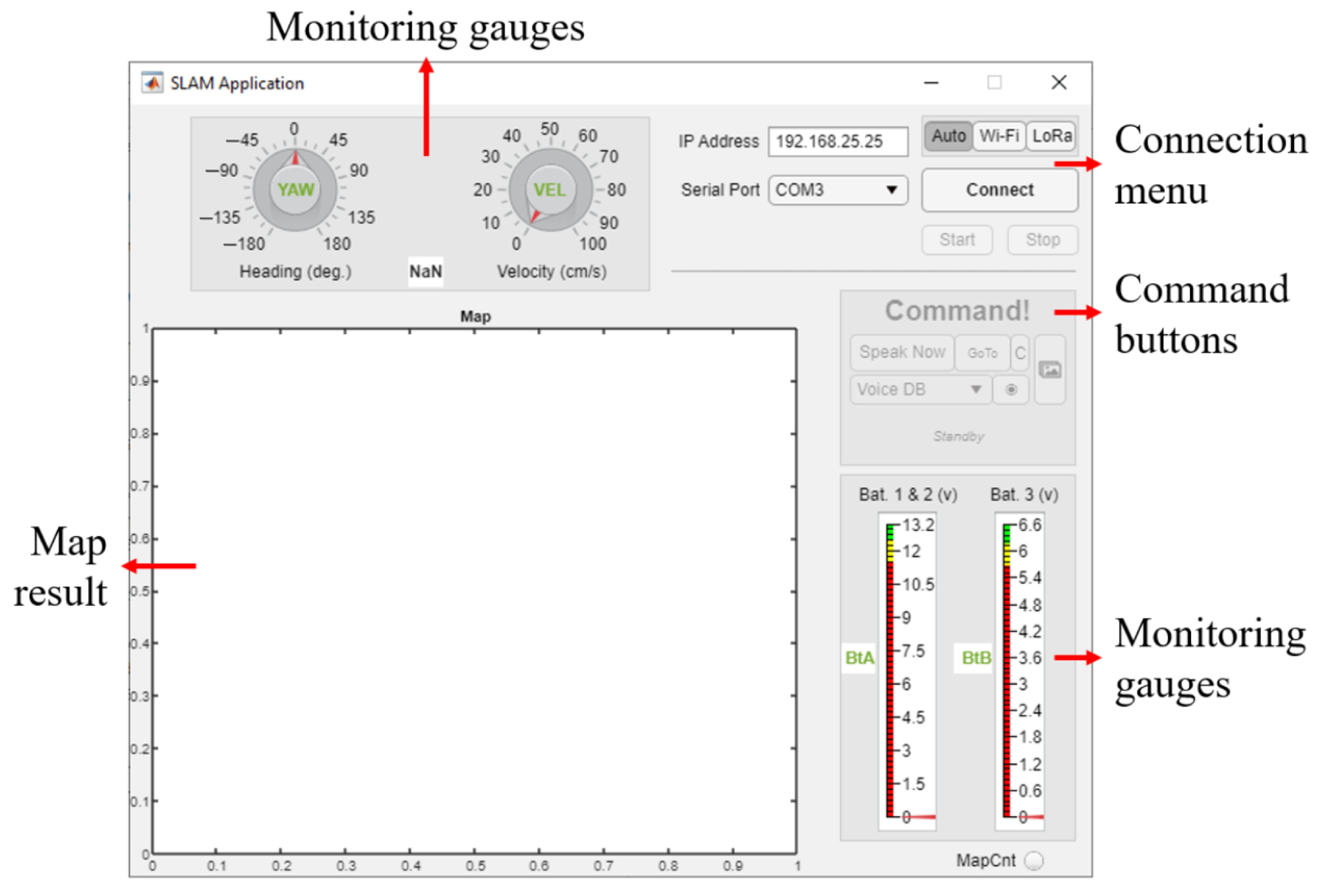
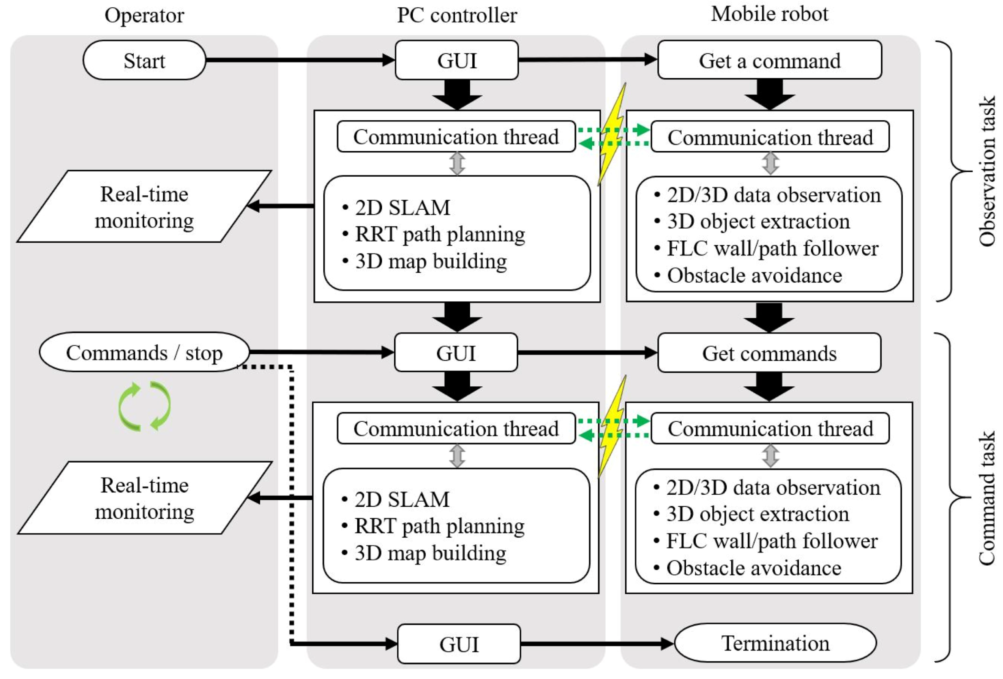
2.2. Software Design

We developed a graphical user interface (GUI) using MATLAB, as shown in Figure 3. The GUI is used by the operator to interact with the mobile robot wirelessly. There are monitoring gauges, a connection menu, command buttons, and a canvas for drawing the map result in real time.
The mobile robot has two missions or tasks, these are the observation task and command task. Figure 4 depicts the task flow in the system. First, the operator starts the mission by using the start button on the GUI. The GUI then sends a start command to the mobile robot for the observation task.
In this task, the mobile robot observes the environment autonomously by sending all observation data to the PC controller. They communicate through the communication thread. This task is intended to build a map for the first time. After finishing the observation, both the PC controller and the mobile robot enter the command task. It enables the command buttons on the GUI, and thus the operator can command the mobile robot based on the first map result. In this task, the mobile robot performs the operator’s commands and all the observation data are also sent to the PC controller to update the map result. This is an iterative task and will be terminated when the operator presses the stop button on the GUI.
In this system, a shared control method is applied. It means that the algorithms are divided to both the PC controller and the mobile robot, as explained in Figure 4. For example, 2D SLAM, a rapidly exploring random tree (RRT) path planning, 3D map building, and GUI are installed in the PC controller. Meanwhile, the mobile robot runs the movement and observation algorithms, such as 3D object extraction, 2D data observation, fuzzy logic control (FLC)-based wall follower and path follower, and obstacle avoidance. This method is especially useful for small robots that are unlikely to carry heavy computers [7]. Furthermore, parallel computing can also be performed. This paper, however, focuses more on the real-time 3D map building using the proposed system, especially with the low-bandwidth communication. In addition, all algorithms in the mobile robot are written in C++, which is preferred for real-time applications.

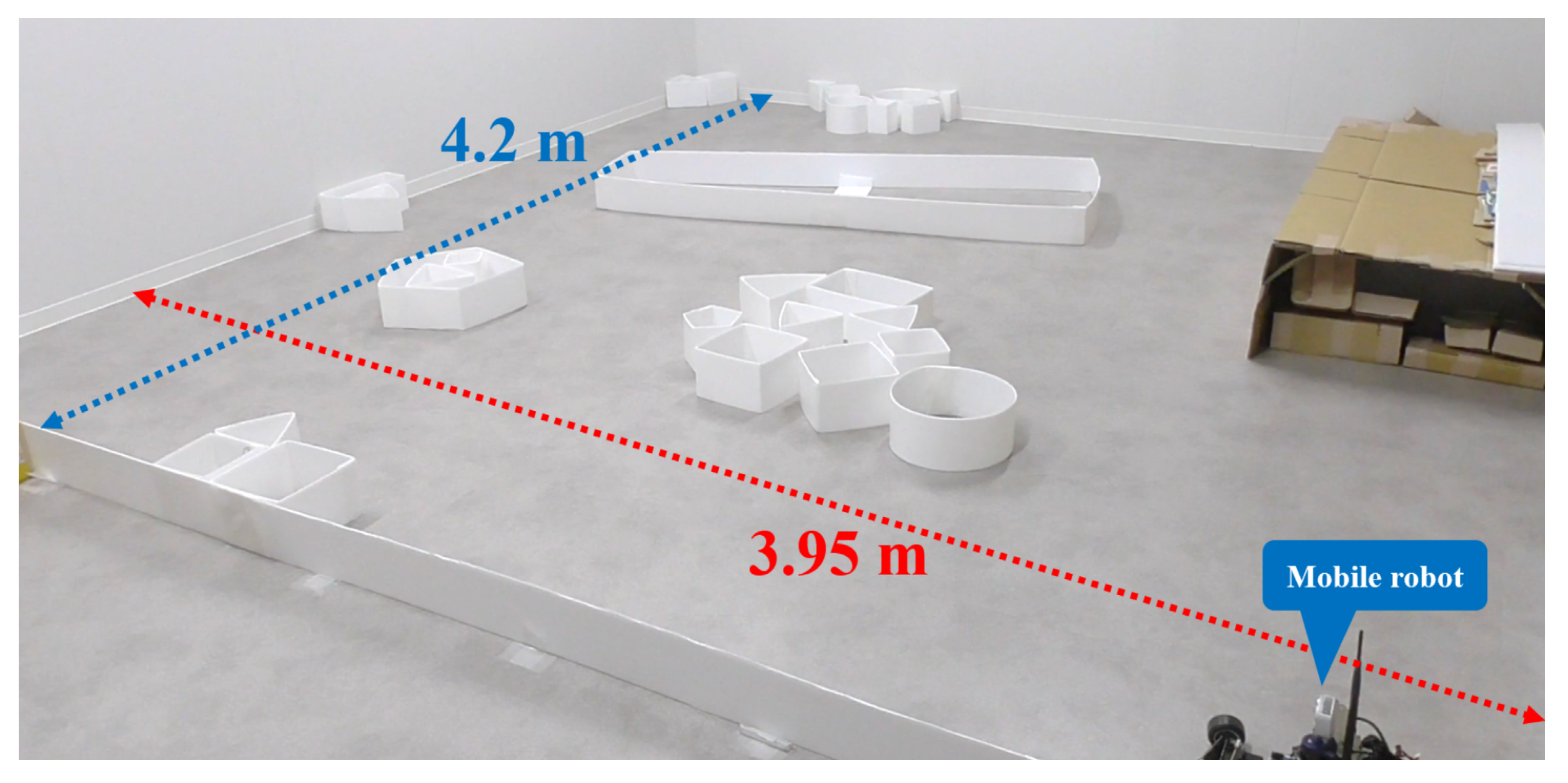
2.3. Experimental Environment

We applied the proposed method for indoor observation in our laboratory. Figure 5 shows the environmental condition. It has 16.59 m2 of large with a lot of cluttered objects inside it. All experiments were carried out in this field, including our datasets for simulation purposes when developing the algorithms. Based on hardware specifications, the objects should have a minimum height of 10 cm, and hence the 2D LiDAR sensor can detect them. In this system, the mobile robot is able to reach an average speed of 0.15 m/s (maximum 0.46 m/s). Therefore, all algorithms need to have real-time capabilities.

3. Proposed Approach

In order to generate a 3D map, 2D SLAM and 3D objects are combined, as depicted in Figure 6. This method enables the system to perform real-time observation even though the low-bandwidth communication is used. The exchanged data can be compressed while maintaining the map accuracy. The next subsections explain important parts of the approach. As mentioned earlier, a shared control method is applied in the system. Therefore, the 3D object extraction algorithm is performed by the mobile robot, while 2D SLAM and 2D–3D combination method are performed by the PC controller.

3.1. 2D Simultaneous Localization and Mapping (SLAM)

Although this paper is focused on real-time 3D map building, it will be difficult to understand without explaining how and what kind of 2D data are used in the system. Hence, this subsection will briefly explain how to observe and manage the 2D data. First, 2D observation data from the LiDAR sensor is compressed for about three-time downsampling [40]. The main reason is, of course, the use of LoRa as low-bandwidth communication. This gives the system a balance between data size and map accuracy. Then, the compressed 2D data will be encoded with the 3D data to be sent to the PC controller.
On the PC controller side, we used MATLAB to develop the mapping algorithms. They include 2D SLAM and 2D–3D combination to construct a 3D map. MATLAB uses graph-based SLAM to create a 2D map [41,42]. A pose estimation of the mobile robot may have an error with the real pose, as well as the estimated map since they are related [43]. The error will increase as the mobile robot wanders throughout the environment. They are usually caused by the sensors’ accuracy and the environmental condition. That is why the graph-based SLAM has a loop closure parameter that will always try to correct the errors. It determines whether or not the current mobile robot pose was previously visited. This is calculated within a small radius by matching the current measurement with all the previous measurements. SLAM is also considered as a basic fundamental problem for a truly autonomous robot [20], where a precise pose is needed to build a map, and the map is also needed to estimate the pose. Therefore, the SLAM problem can be formulated as follows:
P x 1 : t , m | z 1 : t , u 1 : t
where P in (1) is the graph-based SLAM probability distribution, xt is the mobile robot pose at a specific time or measurement, m represents the map, zt is observation data from the sensors, and ut is the controls of the system. Both pose and map are unknown, and they can be solved by calculating the observation data at the beginning of the algorithm. Then, probabilistic models of the observation and motion can be formulated as (2) and (3), respectively.
P z t | x t
P x t | x t 1 , u t
where in (2), the observation relates to the pose, and the new pose is described by the previous pose and its control (3). In addition to the pose graph map, MATLAB also has an occupancy grid map as the output of the 2D SLAM algorithm. Figure 7a,b shows an example of both maps.
The occupancy grid map is generated from the pose graph map, where every cell has a probabilistic value ranging from 0 (empty space) to 1 (occupied space). In the 2D–3D combination process, we use both the pose graph map and the occupancy grid map as the references for 3D objects to be combined. The pose graph map generates positions and orientations of the mobile robot relative to the map, and the occupancy grid map generates information of empty, occupied, or untraveled space. In the system, the 2D SLAM is executed every time step to build a 2D map.

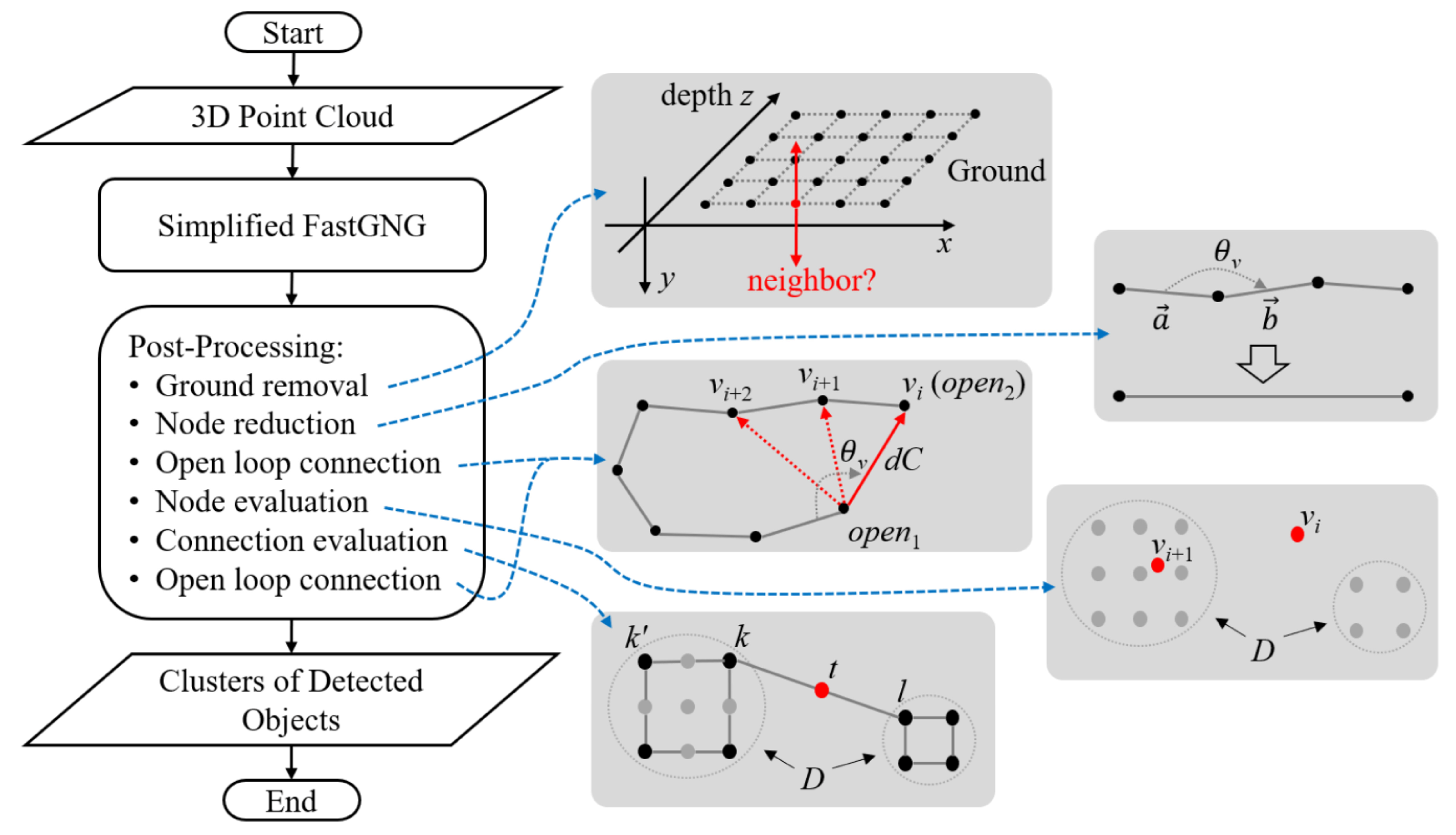
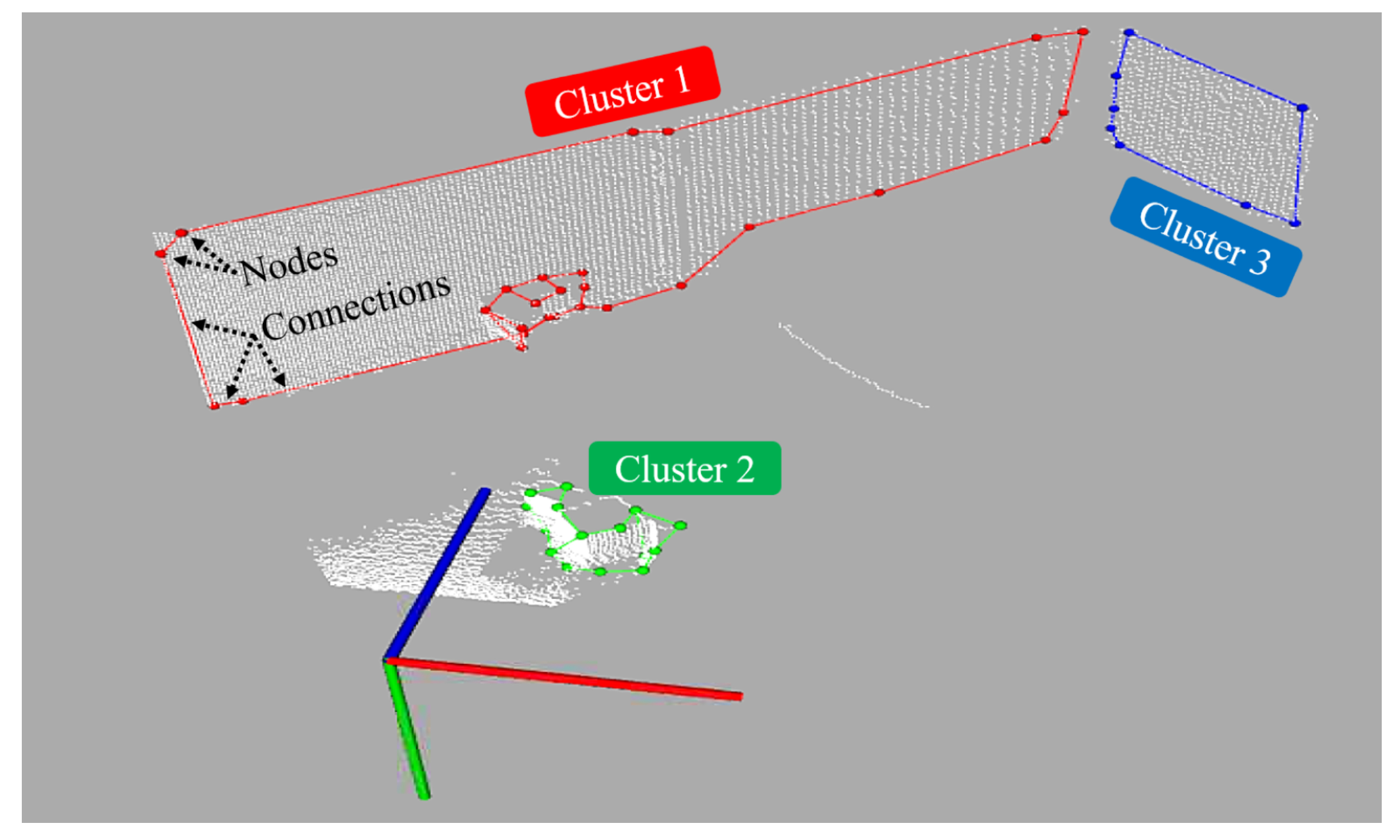
3.2. 3D Object Extraction

The LiDAR camera has two outputs, i.e., color and depth. In this approach, we only use the depth information to extract objects using 3D analysis [44]. Figure 8 shows the image frame projection from the camera.
First, it calculates the real-world coordinates (xc, yc, and zc) using the right-angled triangle principle (4–6).
x c = z g tan x g r e s w 2 F o V w r e s w
y c = z g tan y g r e s h 2 F o V h r e s h
z c = z g
where xg and yg are the pixel coordinate, while zg is the depth measurement at xg, yg. FoVw and FoVh are the camera field of view which are 70° and 50°, respectively. resw and resh are the camera resolutions which are 640 pixels and 480 pixels, respectively.
The 3D object extraction flowchart is shown in Figure 9. We developed a simplification of the fast-growing neural gas (FastGNG) algorithm, called simplified FastGNG, to extract 3D objects from the depth information or point clouds. The standard GNG algorithm uses an iterative method as the learning strategy [45]. Thus, it is difficult to increase the learning speed as a sample node is added to a current network after errors are accumulated with many times of sampling data. FastGNG, on the other hand, is a modification of the standard GNG algorithm, which has a new growing method to enhance the learning speed [46,47]. General objectives such as clustering, feature extraction, and topological mapping can be accomplished using this algorithm.
We proposed a simplification of the FastGNG algorithm to further increase the learning speed and match with the main purpose of this paper. The following are notations used in the simplified FastGNG algorithm:
D
: a set of 3D point cloud data (input);
A
: a set of sample nodes;
w i
: a 3D vector of i-th node;
c i , j
: a connection between i-th and j-th node;
L
: an internal loop parameter of the algorithm;
l m i n , l m a x
: parameters to set the minimum and maximum connection length;
P e d g e ( v )
: the probability of a sample v is the edge, v is a 3D vector;
P n o d e ( v )
: the probability of adding a sample v to the network.
The learning process is then arranged based on following steps:
Step 1. 
Generate a set of sample nodes A using P e d g e ( v ) . This generates edge nodes of the depth input to simplify the learning process. The left, right, top, and bottom node of v should be known. α is a constant. The higher the   α value, the higher the difference in P e d g e ( v ) value between the edge node and the non-edge node. Hence, making it easier to extract the edge nodes.
P e d g e v = max ( e d 1 , e d 2 )
e d 1 = max ( d L d R d L   α , d L d R d R   α )
e d 2 = max ( d T d B d T   α , d T d B d B   α )
d L = v w l e f t ( v ) , d R = v w r i g h t ( v )
d T = v w t o p ( v ) , d B = v w b o t t o m ( v )
Step 2. 
Generate two nodes using P n o d e ( v ) and connect them. Initially, set l m i n and l m a x to any proper value with a constant β , where a higher value results in a higher probability value. Then, initialize the phase level iP to 1.
P n o d e v = 1.0                                                   l m i n d S 1 l m a x 0.0                                                   d S 1 < l m i n                             tanh β l m a x d S 1               otherwise                              
d S 1 = v w s 1 , s 1 = arg   min i A v w i
c n o d e 1 , n o d e 2 = 1 ,   i P = 1
Step 3. 
Initialize the internal loop counter iL to 0 and calculate the l m i n , l m a x , and L.
l m i n = γ 1             i P = 1 γ 2             i P = 2 γ 3             i P 3 , l m a x = δ 1             i P = 1 δ 2             i P = 2 δ 3             i P 3
L = ceil # A σ 1             i P = 1 ceil # A σ 2             i P = 2 ceil # A σ 3             i P 3
where γ i , δ i , and σ i (i = {1, 2, 3}) are constants for l m i n , l m a x , and L, respectively. We set higher values of γ i , δ i , and lower values of σ i for a lower phase. Thus, l m i n and l m a x values are the opposite of the phase level iP. This will speed up the learning process in the first phase, and be slower but more detailed in the higher phases. #A is the number of sample nodes.
Step 4. 
Generate a new node v using P n o d e ( v ) (12) and increase the loop counter iL. Then, calculate the nearest node s 1 (13) and the second nearest node s 2 .
i L = i L + 1
s 2 = arg min i A \ { s 1 } v w i
Step 5. 
Add the new node v (step 4) to the network with a new index r, and update the connection c. Skip the connection if it already exists. Go to step 4 if iL is less than L.
w r = v
c c s 1 , r = 1 , c s 2 , r = 1 , c s 1 , s 2 = 0               d S 1 < d S 12 > d S 2 c s 1 , r = 1 , c s 1 , s 2 = 1                                               otherwise                            
d S 12 = w s 1 w s 2
d S 1 = v w s 1 , d S 2 = v w s 2
Step 6. 
If there are nodes having more than two connections, remove the longest connection. Repeat the removal process until all nodes have a maximum of two connections.
Step 7. 
As a result of the connection deletion in step 6, remove the nodes having no connection at all, and increase the phase level iP. Stop the process when the stopping criteria are satisfied or iP is more than the max_phase parameter. Otherwise, return to step 3.
i P = i P + 1
Now, let us move to the post-processing methods. These are as important as the simplified FastGNG in compressing the depth information and correcting defects from the previous step.

3.2.1. Ground Removal

In this system, we need to remove the ground nodes since we already have the ground information from the 2D SLAM. The set of the 3D point cloud data D is needed for this calculation.
G n d v = 0           d G x < g x d G y > g y d G z < g z 1           otherwise                                                                                        
d G x = v x w i x , d G y = v y w i y , d G z = v z w i z , i D
where g x , g y , and g z are the thresholds based on the minimum distance between input nodes. The ground nodes having G n d v = 1 are then removed from their network. They basically have no neighbors on the y-axes, and hence we use this information to determine the removal process.

3.2.2. Node Reduction

This method reduces the nodes in a straight connection to further compress the point cloud data. Thus, an angle between two connections θ v is used.
θ v = cos 1 a   b a   b
Vector a and b can be known from the corresponding nodes as they have xyz-value. If θ v is more than a specific threshold, i.e., 160°, the corresponding node can be removed and its connections should be updated.

3.2.3. Open Loop Connection

A perfect detection should have closed loop networks around the detected objects. Hence, this method is performed to close the open loop networks. The probability of a node v to be connected to the open loop nodes, P o p e n ( v ) , is defined as follows:
P o p e n v = η 1   θ v + η 2   d C
d C = v w o p e n i ,   i A
where θ v is the same as (26). By using a positive value of η 1 and a negative value of η 2 , the P o p e n ( v ) prioritizes nodes having a larger angle and shorter distance to be a closed loop. Then, the node having the highest P o p e n ( v ) value is connected to the open loop nodes for closing the network.

3.2.4. Node Evaluation

This method is applied to reduce noises and false detection problems. The node evaluation Ne(v) is defined as follows:
N e v = μ = μ + 1               d N x n x d N y n y d N z n z μ = μ                           otherwise                                                                                          
d N x = v x w i x , d N y = v y w i y , d N z = v z w i z , i D
The counter μ is initialized as 0. The node v should be removed if the μ is less than a specific threshold. This means that the node v does not have a sufficient number of neighbors from the input data D. The thresholds nx, ny, and nz are set based on the minimum distance between input nodes of the point cloud.

3.2.5. Connection Evaluation

A connection from a node k to l can be evaluated as follows:
C e k , l = 1           d Q x > q x d Q y > q y d Q z > q z 0           otherwise                                                                                        
d Q x = t x w i x , d Q y = t y w i y , d Q z = t z w i z , i D
t x = k x + l x 2 , t y = k y + l y 2 , t z = k z + l z 2
The same as before, the thresholds qx, qy, and qz are set based on the minimum distance between input nodes. This method compares the center point t of a connection to the input reference D. Therefore, bad connections having C e k , l = 0 are removed from the network.
The output of the 3D object extraction is clusters, consisting of nodes and connections, as shown in Figure 10.
Every node and connection are then encoded to be sent from the mobile robot to the PC controller. From more than 10,000 points in a point cloud to only less than 100 outputs (nodes and connections), a high compression ratio can be achieved using this method, which is especially useful for low-bandwidth communication.
FastGNG adds new nodes after mini-batch learning using weight parameters. Although it improves the learning speed in comparison to the original GNG algorithm, this also results in unnecessary nodes being added to the network, which requires an additional node deletion process. Hence, the simplified FastGNG avoids that by improving the correctness of the probability functions ( P e d g e ( v ) , P n o d e ( v ) ), resulting in additional computational cost savings (see the comparison in the experimental results). Furthermore, due to the higher correctness of the probability functions, a new node and its connections can be added to the network in each step without a node deletion process (steps 4 and 5). Moreover, it also filters the point cloud data at the beginning of the algorithm by applying P e d g e ( v ) to improve the correctness of the sample nodes. Those are the main differences between simplified FastGNG and the FastGNG algorithm. We simplified it from a general-purpose algorithm to a specific purpose in this system.

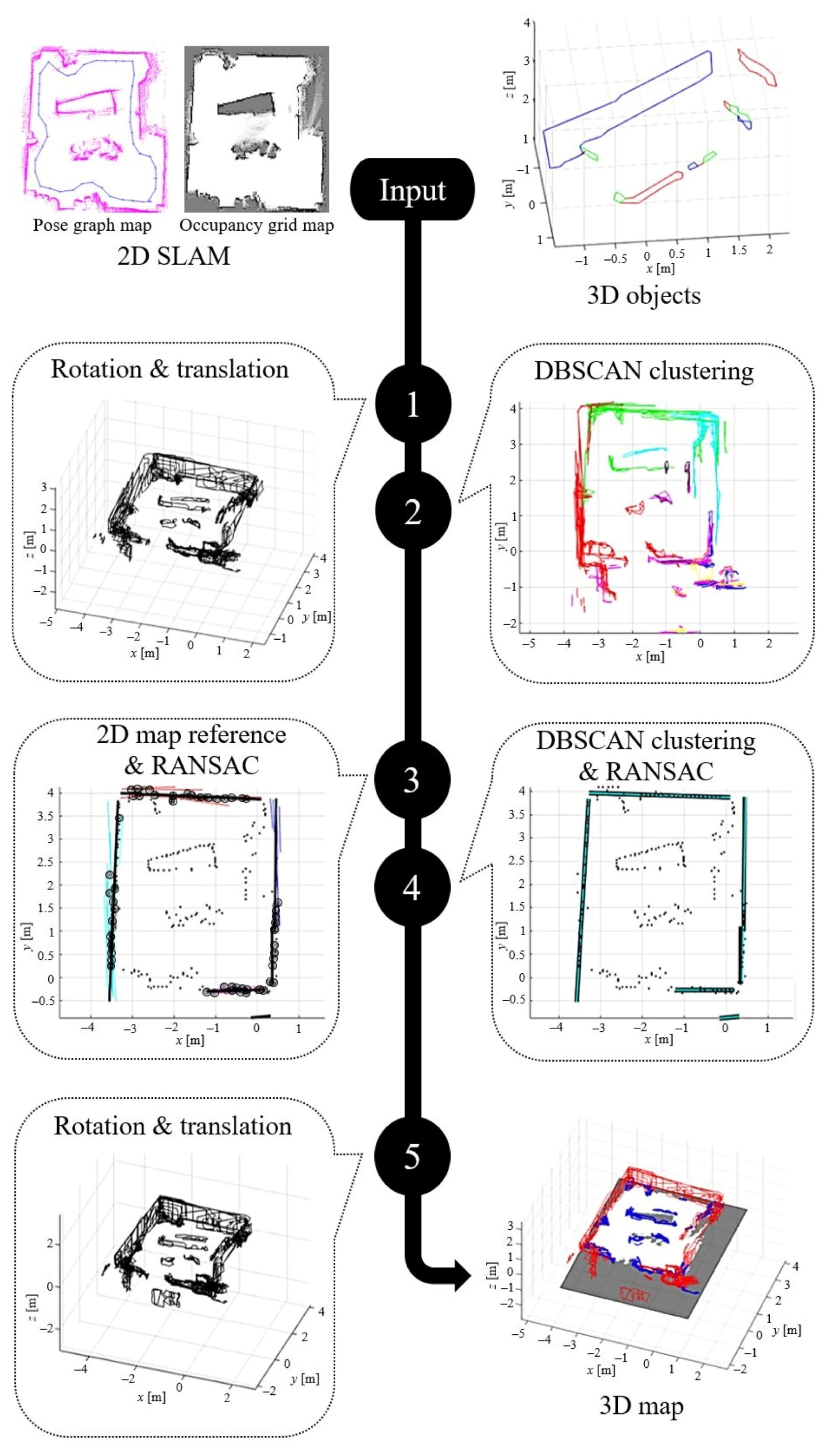
3.3. 2D–3D Combination

The combination process between 2D SLAM and 3D objects is expressed in Figure 11. It starts from rotation and translation with 2D SLAM as the reference. All 3D objects from the simplified FastGNG algorithm are combined based on their clusters to create a new 3D map. Several clustering methods are also employed in the reconstruction process. The following are the steps of the combination process:
Step 1. 
The pose graph map of 2D SLAM generates the orientations ( θ i c ) and 2D position (txi, tyi) that are used for the input references of the rotation (34) and translation (35), respectively. tzi are always zero as the mobile robot only moves on a 2D slat surface.
x y z 1 = cos θ i c sin θ i c 0 0 sin θ i c cos θ i c 0 0 0 0 1 0 0 0 0 1 x y z 1
x y z 1 = 1 0 0 t x i 0 1 0 t y i 0 0 1 t z i 0 0 0 1 x y z 1
In the equation, x, y, and z are the node coordinates of 3D objects. Meanwhile, the double-apostrophe values are the results of this step. The rotation is completed first, and then followed by the translation.
Step 2. 
A density-based spatial clustering of application with noise (DBSCAN) is performed to make a correction of the first rotation and translation results. From the top point of view, a single 3D object may have an L-shape or a non-linear shape. Therefore, a density-based clustering algorithm is needed, and DBSCAN is a pioneer of density-based clustering algorithms [48]. DBSCAN is still being adopted in modern techniques due to its simplicity and compactness for topological clustering applications [49]. The DBSCAN clustering is explained in Algorithm 1. In this method, we convert every 3D object into a 2D line from the top point of view. It simplifies the clustering method since the z values are always correct. The mobile robot never moves on the z-axes. Thus, only x and y values need to be corrected. There are several parameters used in the DBSCAN clustering, such as minObj for a minimum number of objects, dEps for minimum search radius, and thetaTh for rotation threshold. The object rotation angle θ o is calculated using its gradient value (36), and the distance between objects ε is calculated using the Euclidean distance (37).
θ o = tan 1 P 2 y P 1 y P 2 x P 1 x
ε = ( P 2 x P 1 x ) 2 + ( P 2 y P 1 y ) 2
where P1 and P2 are two points in a single object as an xy-line. The output of this step is the clusterObj (colored lines in Figure 11 step 2) that will be used in the next step, and noiseObj (black lines in Figure 11 step 2) that is removed from the map result.
Step 3. 
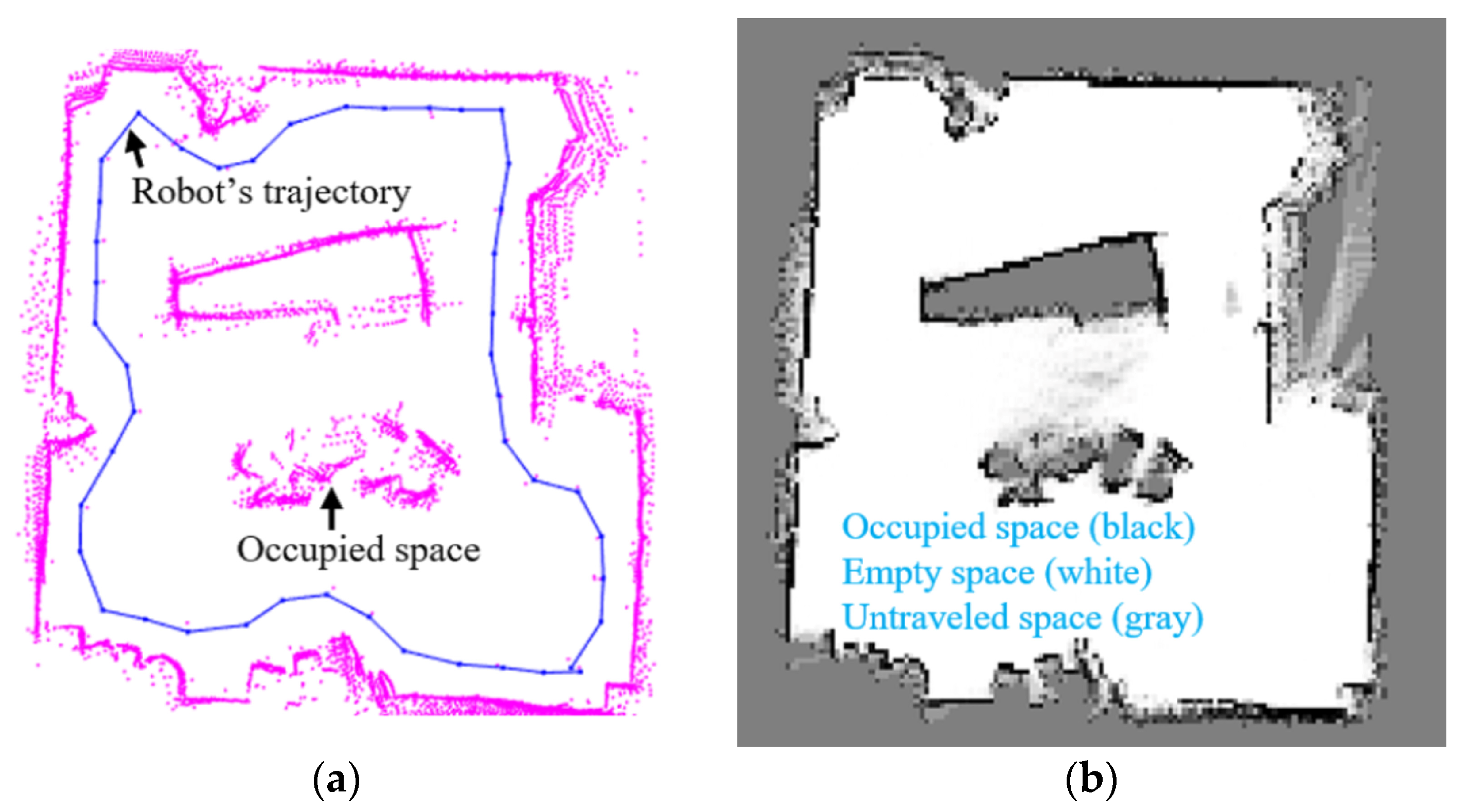
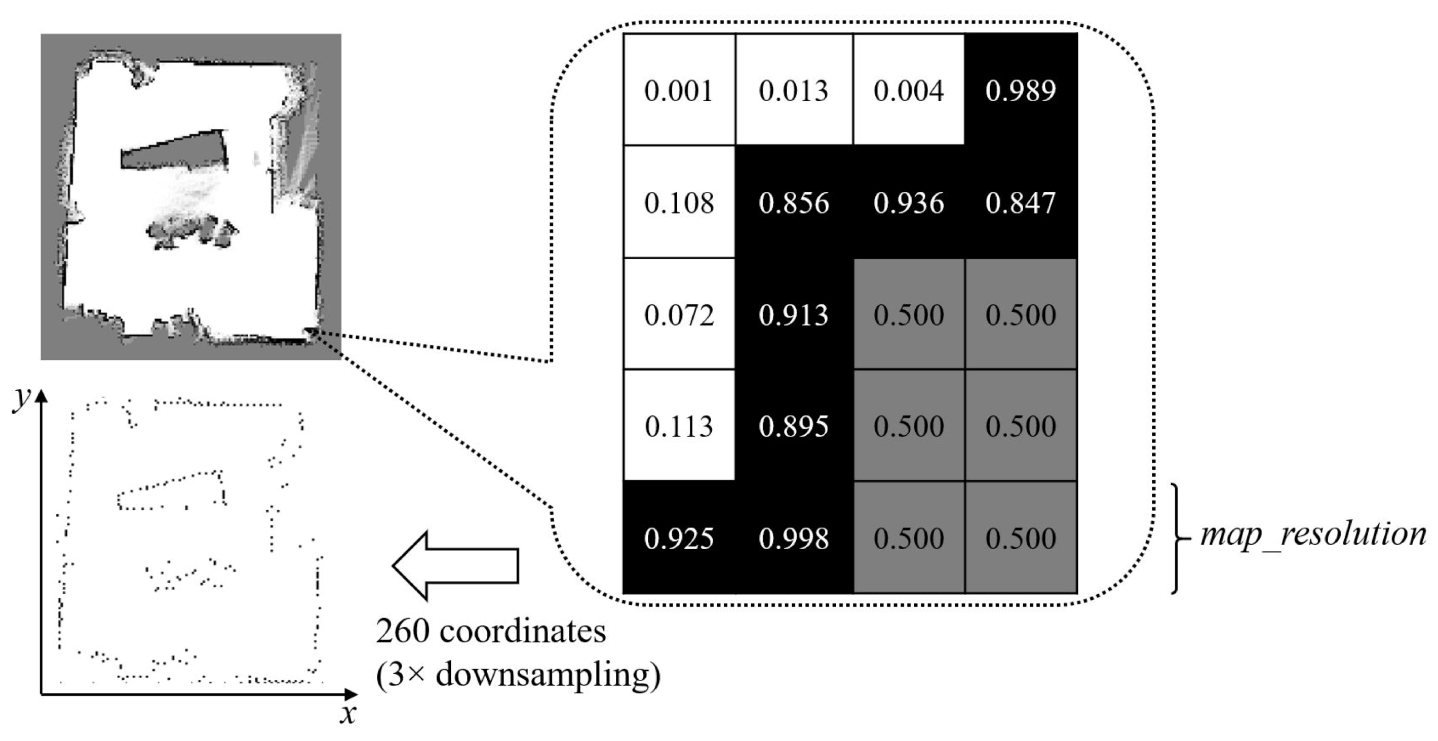
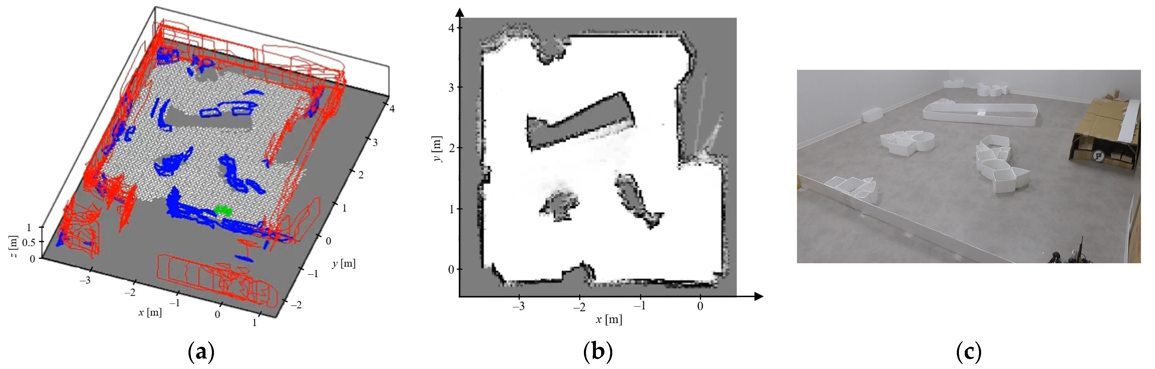
The pose graph map of 2D SLAM only generates orientations and positions of the individual map displacements. In other words, they are the mobile robot orientations and positions when scanning the environment or capturing the data. Therefore, to generate a 2D map reference, the occupancy grid map from 2D SLAM is used, as shown in Figure 12. It is generated based on the values of the occupancy grid map, where empty space is represented by low values (near 0), occupied space has high values (near 1), and untraveled space is between 0 and 1 (0.5 initially). We set 0.750 as the threshold to generate the 2D map reference. All nodes of the 2D map reference are then compared to the DBSCAN clustering result. By using a specific threshold, i.e., the Euclidean distance, these nodes can all be known to which DBSCAN cluster they belong. They are shown as black circles in Figure 11 step 3.
Algorithm 1: DBSCAN Clustering
Input:sampleObj, thetaTh, dEps, minObj
Output:clusterObj, noiseObj
clusterObj ← Null
noiseObj ← Null
while True do
   temp_clust ← random(sampleObj)
   isUpdate ← True; l_start ← 1; l_stop ← 1
   while isUpdate do
      isUpdate ← False
      for il_start to l_stop do
         coretemp_clusti
         for j ← 1 to numOf(sampleObj) do
            if |sampleObjj.θcore.θ| ≤ thetaTh and
               distEuc(sampleObjj, core.xy) ≤ dEps then
               temp_clust.add(sampleObjj)
               isUpdate ← True
            end if
         end for
      end for
      l_startl_stop + 1
      l_stop ← numOf(temp_clust)
   end while
   if numOf(temp_clust) ≥ minObj then
      clusterObj.add(temp_clust)
   else
      if numOf(temp_clust) = 1 then
         noiseObj.add(temp_clust)
      else
         clusterObj.add(temp_clust)
      end if
   end if
   if numOf(noiseObj) + numOf(clusterObj) = numOf(sampleObj) then
      break
   end if
end while
return clusterObj, noiseObj
Random sample consensus (RANSAC) [50] is then performed to generate 2D reference lines (black lines in Figure 11 step 3) based on the 2D map reference and the cluster. The line equations used in the RANSAC are as follows;
y r s c = m r s c x r s c + b r s c
m r s c = y 2 y 1 x 2 x 1
θ r s c = tan 1 m r s c
The slope m r s c is calculated using the gradient value of two sample points, (x1, y1) and (x2, y2). Then, its y-intercept b r s c can be known from the sample point ( x r s c , y r s c ), and its angle θ r s c can be known from the m r s c value. This process is also explained in Algorithm 2.
Step 4. 
In this step, DBSCAN clustering is performed to the RANSAC results of step 3. It generates new clusters for the 2D map reference nodes as a correction of the previous results. Next, RANSAC is applied to the new clusters to generate new 2D reference lines (light blue lines in Figure 11 step 4). These 2D reference lines are used as the final references to rotate and translate all 3D objects in the last step.
Step 5. 
All 3D objects are re-rotated and re-translated using the last references from step 4. It is a correction of the rotation and translation in the first step. Finally, ground information from the occupancy grid map of 2D SLAM is combined with the result of this step. This is the final rendering result of 3D surface reconstruction, as shown in Figure 11.
As described in Figure 6, the 2D–3D combination is run on the PC controller. Since the 2D SLAM tends to accumulate errors before a loop closure, this process is executed every three time steps after the loop closure is detected. On the mobile robot, both 2D and 3D data are captured at the same time, and thus they represent the same object. However, due to sensors and the object extraction accuracy, they are not exactly aligned. Therefore, we performed an alignment process in the 2D–3D combination method to improve the 3D map accuracy.

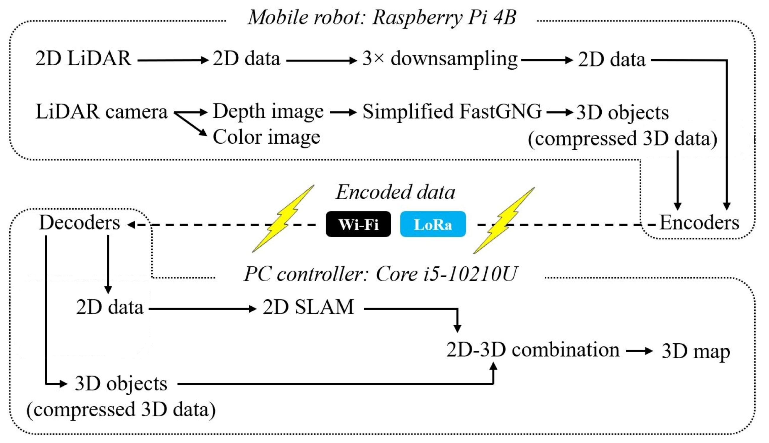
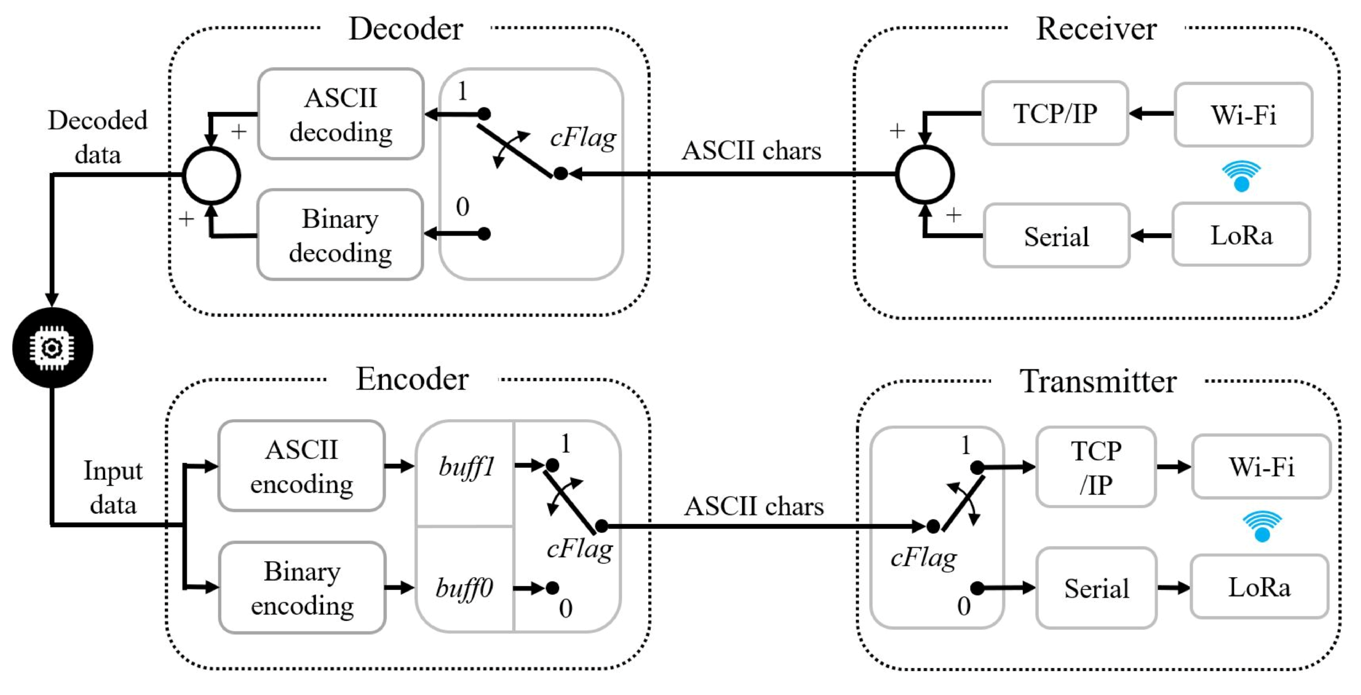
3.4. Communication System

The combination of Wi-Fi and LoRa is configured based on each communication protocol, i.e., transmission control protocol/internet protocol (TCP/IP) and serial protocol, respectively. Figure 13 depicts the communication system architecture. The connection manager algorithm manages all network switching processes using a cFlag parameter, as explained in Algorithm 3.
Algorithm 2: RANSAC
Input:sampleData, maxIteration, inliersTh
Output:bestM, bestB, bestTheta
maxInliers ← –1
fori ← 1 to maxIteration do
   rand1 ← random(sampleData)
   rand2 ← random(sampleData)
   while rand1 = rand2 do
      rand2 ← random(sampleData)
   end while
   mrsc r a n d 2 . y r a n d 1 . y r a n d 2 . x r a n d 1 . x
   brscrand1.ymrsc rand1.x
   θrsc tan 1 m r s c
   countInliers ← 0
   for j ← 1 to length(sampleData) do
      if |θrsc| ≤ 45.0 then
          newXsampleDataj.x
          newYmrsc newX + brsc
      else
          newYsampleDataj.y
          newX n e w Y b r s c m r s c
      end if
      dist ← distEuc(new.XY, sampleDataj)
      if distinliersTh then
          countInlierscountInliers + 1
      end if
   end for
   if countInliers > maxInliers then
      maxInlierscountInliers
      bestMmrsc
      bestBbrsc
      bestThetaθrsc
   end if
end for
return bestM, bestB, bestTheta
In addition, different encoding and decoding strategies are applied to the system, i.e., ASCII coding for Wi-Fi and binary coding for LoRa, which are not the focus of this paper. The reason for using ASCII coding for Wi-Fi is that the 2D LiDAR output is already in ASCII format, and the data size can be compensated by the Wi-Fi bandwidth (353 kbps–9 Mbps). On the other hand, binary coding is required for LoRa to compress all data as it has low bandwidth (6.01 kbps–22 kbps). Therefore, real-time applications can be performed by the system using both communication bandwidths.
Algorithm 3: Connection Manager
Input:IPaddr, tcpPort, tcpTimeout, comPort, serBaud, serTimeout
Output:cFlag
connTCP ← tcpconfig(IPaddr, tcpPort, tcpTimeout)
connSer ← serconfig(comPort, serBaud, serTimeout)
cFlag ← 1
while True do
   if cFlag = 1 then
      try
         funcTxRx(connTCP)
      catch
         cFlag ← 0
      end try
   else
      funcTxRx(connSer)
   end if
end while

4. Results and Discussion

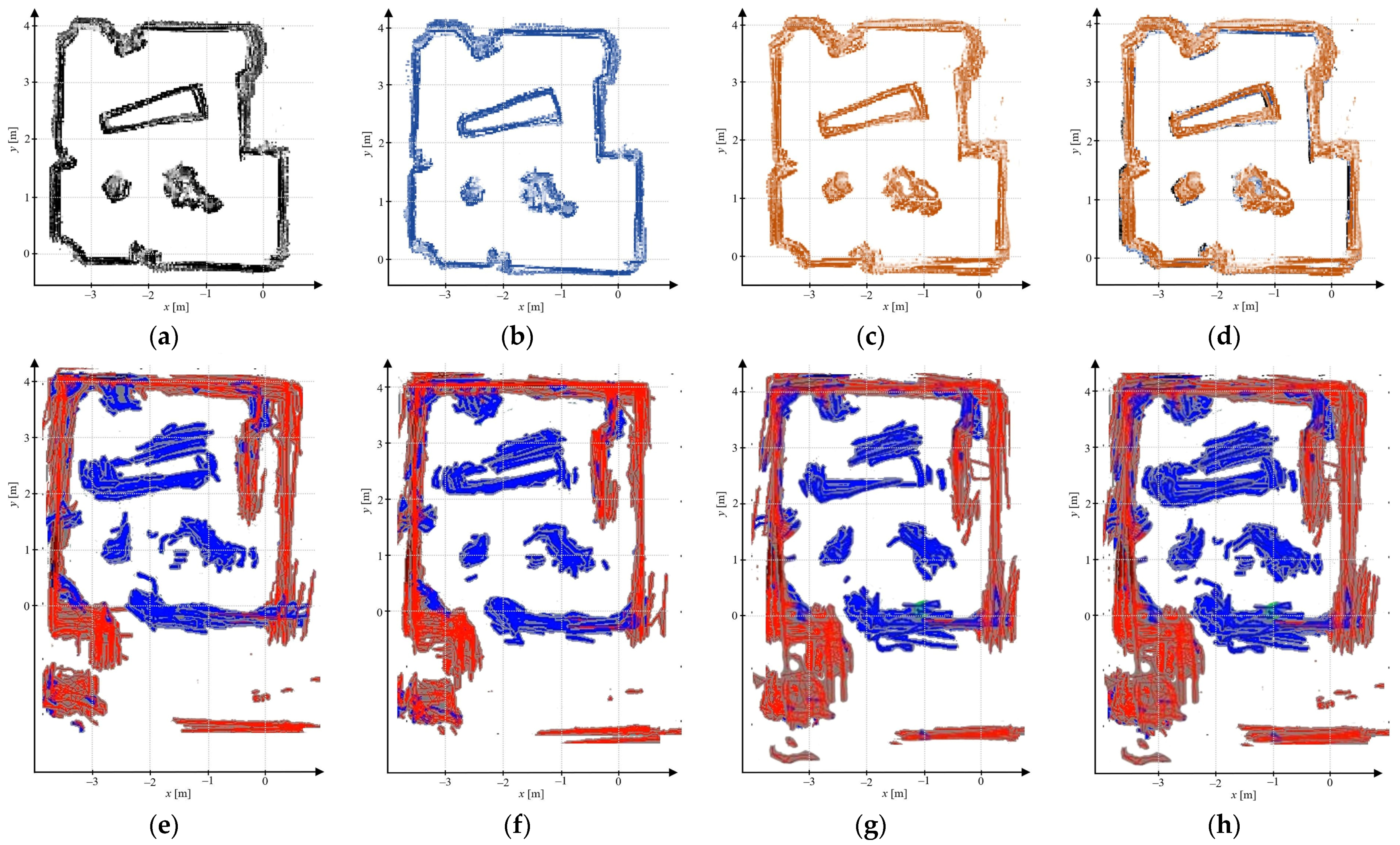
4.1. 3D Object Extraction Evaluation

First, the standard GNG algorithm, FastGNG, and simplified FastGNG were compared for the same input dataset in our laboratory. All ran the object detection without post-processing methods. Table 2 summarizes the results.
It is difficult to run for the same number of nodes in each trial, especially for FastGNG and simplified FastGNG, since they use phase level (iP). Based on the results, the standard GNG algorithm has the highest computational cost. It really depends on the number of iterations. On the other hand, the FastGNG algorithm runs faster. It is roughly three times faster than the standard GNG algorithm. The simplified FastGNG has a similar performance as the FastGNG. It uses the same core as in the FastGNG algorithm, however, in a simpler way, to achieve improved performance for the proposed system. In this case, we set the max_phase = 3 as the limit.
In order to evaluate the performance of the 3D object extraction method, 3D point cloud datasets from our laboratory were used. The datasets, which have the same resolution of 640 × 480 pixels, were previously recorded using the LiDAR camera as described in Section 2.1. All parameter settings for the evaluation can be seen in Table 3. Figure 14 shows the detection results, while the performance is summarized in Table 4. In the experiments, all post-processing methods were also performed. Based on the results, the proposed method can achieve the mean performance of 31.15 fps. That will be difficult to achieve when using the standard GNG algorithm, which has the mean execution time of 67.9 ms (14.73 fps) without any post-processing methods. This implementation is necessary, as we need to maintain all algorithms to be real-time capable in order to realize the target of this system.
Another important thing is the data compression. Remember that we need to send all monitoring data using both Wi-Fi and LoRa networks. It is impossible to send all raw-point cloud data using low-bandwidth communication. Due to bandwidth restrictions, real-time performance will not be achieved, and there will be a data loss problem. Thus, the simplified FastGNG solves the problem by compressing the data size while at the same time maintaining its performance in real time. The trade-off is, of course, the map quality. Higher compression results in faster data transmission time but lower map quality, and vice versa. However, compared to our previous work using particle swarm optimization-seeded region growing (PSO-RG) [51], which has a mean performance of 11.3 fps, the simplified FastGNG offers a better balance between data compression, accuracy, and computational cost. Furthermore, the PSO-RG limits each cluster to only eight nodes, which is much less than the simplified FastGNG results (48–80 in Table 4), making it more accurate to represent the detected objects. Even though the data size is approximately six to ten times larger, the communication bandwidth can still handle it.

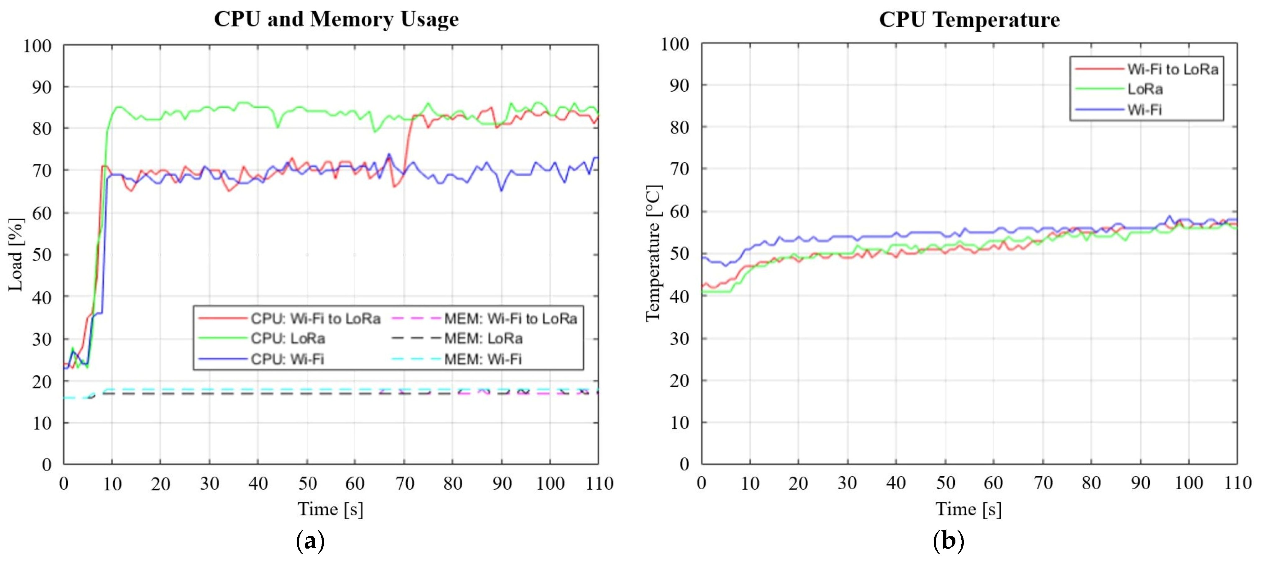
4.2. Real-Time Experimental Results

We performed fifteen trials to evaluate the proposed methods. All of them were run on the proposed system in real time. There are configurations of Wi-Fi to LoRa, LoRa only, and Wi-Fi only, each of which are conducted five times. The environmental condition for experiments is shown in Figure 5. However, the placement of the objects in it may change. The parameter settings for the experiments are shown in Table 5. These parameters are used in the 2D–3D combination method to build a 3D map.
Table 6 shows the computational costs of the experiments. The mobile robot observes 2D and 3D data in parallel, and hence the computational cost in it will be the longest time. Figure 15 depicts the 3D map results (Figure S1). In Figure 15a, the mobile robot performed both the observation task and the command task. Therefore, the mobile robot final position is different from Figure 15b,c, which only performed the observation task. Similarly, the map density is also different due to the difference in the amount of data sent by the mobile robot to the PC controller. In the experiments, the mobile robot reached an average speed of 0.15 m/s (maximum 0.46 m/s), which depended on the track length and obstacles.
Figure 16 explains the missions of Figure 15a step by step, where the system switched the network automatically from Wi-Fi to LoRa in the middle of the observation task (Video S1). Then, in the command task, the operator commanded the mobile robot to go to a specific position in the map by using the command buttons on the GUI. Of course, there are some delays for monitoring data when using the LoRa network compared with the Wi-Fi network. This is caused by the low bandwidth of LoRa.
Based on the results in Table 6, the data transmission time is different among different network configurations, and obviously Wi-Fi is the fastest network. The 2D SLAM and 2D–3D combination are performed in the PC controller, and hence they all have similar results. Lastly for data size, as mentioned earlier, we used different strategies for data coding methods between Wi-Fi and LoRa networks. ASCII coding is used for Wi-Fi and binary coding is used for LoRa. Therefore, the mean LoRa data size is smaller than the mean Wi-Fi data size. When using the Wi-Fi to LoRa configuration, the data are coded either using ASCII or using binary coding corresponding to the current network that the system uses. On the mobile robot side, there are two kinds of data sent to the PC controller, i.e., 2D and 3D data. A three-time downsampling is applied to the 2D data and the simplified FastGNG is applied to the 3D data to extract 3D objects. These result in a total maximum computational cost of 799.1 ms, which is 1.25 Hz. Thus, the operator can obtain the map update for at least 1.25 Hz for monitoring data. Faster updates can, of course, be achieved when the system uses the Wi-Fi network.
To evaluate the map results, we combined all fifteen maps and plotted them in 2D from the top point of view, as shown in Figure 17. Since the mobile robot only moves in 2D space, only the x and y-axes need to be evaluated. Compared to the ground truth in Figure 15d, they have about the same shape and size, which are 3.95 m in width and 4.2 m in length. At the same time, the results show that the proposed method has good repeatability from all fifteen trials with different network configurations.
There is one more scenario for the system to perform real-time observation and 3D map building. Figure 18 depicts the map results. The environmental condition is the same but with different object placements. The LoRa network was used and resulted in similar performance as in Table 6. These results also confirm the feasibility of the proposed method for performing real-time 3D map building under the system restrictions.

4.3. Discussion

In order to achieve real-time application of the system, all implemented algorithms need to have real-time capabilities, as depicted in Figure 6. The more data for the algorithms, the higher the accuracy of the results. However, the computational costs may also increase. Therefore, it is very important in this system to maintain a balance between the amount of data and its accuracy. In mobile robot operations, at least an operator is needed not only to control, but also to monitor the mobile robot’s behaviors in performing the missions. Hence, real-time capabilities should be considered since they enable not only direct results, but also real-time responses between the operator and the mobile robot. In [22], it defines a real-time target for 3 s. This paper, however, is targeted at 1 s (1 Hz). We considered it based on the implemented hardware in the system, and it was confirmed by the experimental results.
As depicted in Figure 4, there are several tasks running in parallel on the mobile robot while observing the environment. The FLC wall path follower and obstacle avoidance are running in the background to handle the mobile robot’s movements. Regarding the mobile robot speed, we defined in the FLC controller that 0.2 m/s is the medium speed, less than 0.1 m/s is the slow speed, and more than 0.4 m/s is the fast speed. Based on the experimental results, the mobile robot is able to reach a maximum speed of 0.46 m/s with an average speed of 0.15 m/s. This is a car-like mobile robot, and thus it also needs to go backward to avoid the obstacles. All the above experiments, of course, run in parallel with the background programs. In addition, we also installed an active cooling fan to maintain the Raspberry Pi CPU temperature. Figure 19 shows the CPU performance when running the missions. There are configurations of Wi-Fi to LoRa, LoRa only, and Wi-Fi only. The missions were started at around 5 s, and then both CPU temperature and CPU usage started to rise. When using the Wi-Fi network, the CPU usage is lower than when using the LoRa network. This is caused by the program architecture. One additional thread is added for the LoRa network to help the communication thread. It performs timeout recovery algorithms to prevent data loss on the LoRa network [40], as all data are important for the mapping process. It is worth noting that when the CPU temperature rises to 80–85 °C, the CPU will start to slow down and reduce all clocks, as written in the Raspberry Pi documentation. In the worst case, the simplified FastGNG algorithm may drop to 10 fps when the CPU throttling happens. Hence, the implementation of the active cooling is very important.
Modern SLAM algorithms, such as ORB-SLAMs [29,30,31], can also run in real time on embedded systems [32,33]. Since they require three or more threads to achieve real-time performance, it is difficult for this system to be implemented. Instead, we run the mapping algorithms on the PC controller and focus the mobile robot on data observation. Under embedded systems, ORB-SLAMs can achieve a performance of 2.2–12.69 fps (454–79 ms) [32]. If we only compare the mapping algorithms, the proposed method can perform competitively, which is 8.9–10.2 fps (112–98 ms in Table 6).
In contrast to [28], which prioritizes quality and repeatability, this paper prioritizes repeatability (Figure 17) and real-time performance under low-cost hardware limitations to perform 3D mapping. This is one of our novelties, as most of the state-of-the-art focuses on how to construct a 3D map for better quality but ignores real-time processing [23,24,25]. This will make real-time control and observation difficult to realize, even more so for low-cost devices. Of course, this is a trade-off between data size, accuracy, and computational cost. In this paper, we balance all of them to achieve the target of the proposed system. Thus, the drawback of this work is map quality, as it is nearly impossible to send the amount of data under low-bandwidth communication in real time.
The advantage of our proposed approach is the use of low-bandwidth communication. The combination of high and low-bandwidth networks is also developed in [2,32]. All of them confess that the network combination improves the robustness of wireless communication for mobile robot applications. However, they still require the high-bandwidth network to build a full 3D map and complete the missions. Our system, on the other hand, enables complete network switching. This means that all observation data for 3D mapping can be sent to the host using either the high or low-bandwidth network, even when the main network is completely lost. This brings us to another novelty of this paper, as, to the best of the authors’ knowledge, there are no similar works performing real-time 3D map building under low-bandwidth networks.
The first step of the 2D–3D combination method, rotation and translation, is actually sufficient to represent the environment as a 3D map. The reason for applying the other processes is accuracy. Next, RANSAC is also a bit time consuming. In this case, we set the maxIteration parameter to 1.5 n, where n is the number of sample data.
As explained in Section 2, C++ is used in the mobile robot and MATLAB is used in the PC controller. MATLAB has a MATLAB Coder, which generates C/C++ code directly from MATLAB code. This is very important to be implemented as it can run more than ten times faster than native MATLAB code. Table 6 shows how fast the algorithms (2D SLAM and 2D–3D combination) can be executed by the PC controller.
The challenge of the proposed approach is the number of parameters. We found that it is difficult to obtain appropriate results without understanding the input data characteristics. We have to set the parameters step by step based on the purpose of each algorithm. It is difficult to jump to the next parameters if the previous parameters are not stable yet. For example, setting the parameters for six post-processing methods after the simplified FastGNG algorithm. We must first successfully remove the ground nodes before adjusting the second method, and so forth.
The compressed data size for LoRa is around 0.471 KB (mean). This enables a real-time transmission time of 627 ms (625 ms in experiments) with a speed of 6.01 kbps. By using the compression ratio for 2D and 3D data, the raw data size for LoRa can be estimated to be 11.492 KB. It will take around 15.29 s to send the uncompressed data using LoRa, making the real-time target completely impossible when using the low-bandwidth communication. The Wi-Fi transmission speed can also be estimated to be 414.22 kbps, where the data size is 0.932 KB and the transmission time is 18 ms. However, Wi-Fi can certainly perform much faster since it can stream videos in real-time.
There are two restrictions in the proposed system, i.e., limited onboard computing resources and low-bandwidth communication. Compared with [2,22,23,28], it is difficult to achieve the real-time target under those two restrictions. Therefore, we developed the proposed method to address the problems. It proved the ability to achieve the target of 1 Hz refresh rate, which is our design system for enabling real-time control and monitoring for the operator. The combination of Wi-Fi and LoRa makes the system robust against network problems. The developed algorithms are lightweight and can be installed on relatively low-cost hardware. Parallel computing is also performed as the system uses a shared control method to run all the algorithms. Finally, real-time 3D map building can be conducted using both high and low-bandwidth networks.

5. Conclusions

3D visualization of the real world is becoming increasingly important. In robotics, it is not only required for intelligent control, but also necessary for operators to provide intuitive visualization. However, due to the increase in the amount of data, real-time processing is becoming a challenge, even more so for low-cost mobile devices. Therefore, in order to address this problem, we propose a real-time 3D map building based on the combination of 2D SLAM and 3D objects that can be applied to low-cost hardware.
Starting with 2D–3D data observation and 3D object extraction, all observation data are sent wirelessly from the mobile robot to the PC controller to create a 3D map. First, the 2D SLAM algorithm is run by the PC controller to build a 2D map based on the 2D observation data. Then, the simplified FastGNG algorithm, which is run by the mobile robot, compresses 3D point cloud data as 3D objects. It gives the system a balance between data size, accuracy, and computational cost, and thus enables real-time data transmission even though the low-bandwidth communication is used. Lastly, the 2D–3D combination method is applied to create a 3D map in the PC controller. This combines the 2D data from 2D SLAM and 3D objects from the simplified FastGNG algorithm. The low-bandwidth communication using the LoRa network is actually the main target, as it restricts not only the data size, but also the data transmission speed.
The results show that the proposed method can perform a minimum 1.25 Hz refresh rate, which is real-time capable. It means that the operator will obtain the map update for at least 1.25 Hz for one monitoring data. This proves that the target of a 1 Hz refresh rate can be achieved by the proposed method. Of course, a higher refresh rate can be achieved when the system uses the Wi-Fi network.
In addition, the combination of high and low-bandwidth networks also enables the system to maintain its client–server communication. Therefore, the missions can be continued, and real-time monitoring can still be performed even if the system loses the Wi-Fi network completely.
In future work, we will improve the LoRa performance since it is still far from its maximum bandwidth. The data may also need to be compressed using another compression technique that makes it smaller in size. In addition, we want to try more complex environments to see what further improvements are needed for the algorithms.

Supplementary Materials

The following supporting information can be can be downloaded at: https://www.mdpi.com/article/10.3390/robotics12060157/s1, Figure S1: 3Dmaps; Figure S2: GA; Video S1: Demo.

Author Contributions

Conceptualization, A.J. and H.M.; methodology, A.J., H.M., K.S., T.M. and N.T.; software, A.J.; validation, H.M.; formal analysis, A.J., H.M., K.S., T.M. and N.T.; investigation, A.J.; resources, A.J. and H.M.; data curation, A.J. and H.M.; writing—original draft preparation, A.J.; writing—review and editing, A.J. and H.M.; visualization, A.J.; supervision, A.J., H.M., K.S., T.M. and N.T.; project administration, H.M. All authors have read and agreed to the published version of the manuscript.

Funding

This research received no external funding.

Data Availability Statement

The data presented in this study are available on request from the corresponding author within a certain period of time.

Conflicts of Interest

The authors declare no conflict of interest.

References

  1. Guo, B.; Dai, H.; Li, Z.; Huang, W. Efficient planar surface-based 3D mapping method for mobile robots using stereo vision. IEEE Access 2019, 7, 73593–73601. [Google Scholar] [CrossRef]
  2. Schwarz, M.; Rodehutskors, T.; Droeschel, D.; Beul, M.; Schreiber, M.; Araslanov, N.; Ivanov, I.; Lenz, C.; Razlaw, J.; Schuller, S.; et al. NimbRo rescue: Solving disaster-response tasks with the mobile manipulation robot momaro. J. Field Robot. 2016, 34, 400–425. [Google Scholar] [CrossRef]
  3. Tian, Y.; Liu, K.; Ok, K.; Tran, L.; Allen, D.; Roy, N.; How, J.P. Search and rescue under the forest canopy using multiple UAVs. Int. J. Robot. Res. 2020, 39, 1201–1221. [Google Scholar] [CrossRef]
  4. Okada, K.; Kagami, S.; Inaba, M.; Inoue, H. Plane segment finder: Algorithm, implementation and applications. IEEE Int. Conf. Robot. Autom. 2001, 2, 2120–2125. [Google Scholar]
  5. Geromichalos, D.; Azkarate, M.; Tsardoulias, E.; Gerdes, L.; Petrou, L.; Pulgar, C.P.D. SLAM for autonomous planetary rovers with global localization. J. Field Robot. 2019, 37, 830–847. [Google Scholar] [CrossRef]
  6. Yin, H.; Wang, Y.; Tang, L.; Ding, X.; Huang, S.; Xiong, R. 3D LiDAR map compression for efficient localization on resource constrained vehicles. IEEE Trans. Intell. Transp. Syst. 2021, 22, 837–852. [Google Scholar] [CrossRef]
  7. Inaba, M.; Kagami, S.; Kanehiro, F.; Hoshino, Y.; Inoue, H. A platform for robotics research based on the remote-brained robot approach. Int. J. Robot. Res. 2000, 19, 933–954. [Google Scholar] [CrossRef]
  8. Ding, L.; Nagatani, K.; Sato, K.; Mora, A.; Yoshida, K.; Gao, H.; Deng, Z. Terramechanics-based high-fidelity dynamics simulation for wheeled mobile robot on deformable rough terrain. In Proceedings of the 2010 IEEE International Conference on Robotics and Automation, Anchorage, AK, USA, 3–7 May 2010; pp. 4922–4927. [Google Scholar]
  9. Li, W.; Ding, L.; Gao, H.; Tavakoli, M. Haptic tele-driving of wheeled mobile robots under nonideal wheel rolling, kinematic control and communication time delay. IEEE Trans. Syst. Man Cybern. Syst. 2020, 50, 336–347. [Google Scholar] [CrossRef]
  10. Li, Y.; Li, M.; Zhu, H.; Hu, E.; Tang, C.; Li, P.; You, S. Development and applications of rescue robots for explosion accidents in coal mines. J. Field Robot. 2019, 37, 466–489. [Google Scholar] [CrossRef]
  11. Takemori, T.; Miyake, M.; Hirai, T.; Wang, X.; Fukao, Y.; Adachi, M.; Yamaguchi, K.; Tanishige, S.; Nomura, Y.; Matsuno, F.; et al. Development of the multifunctional rescue robot FUHGA2 and evaluation at the world summit 2018. Adv. Robot. 2019, 34, 119–131. [Google Scholar] [CrossRef]
  12. Jeong, I.B.; Ko, W.R.; Park, G.M.; Kim, D.H.; Yoo, Y.H.; Kim, J.H. Task intelligence of robots: Neural model-based mechanism of thought and online motion planning. IEEE Trans. Emerg. Topics Comput. Intell. 2017, 1, 41–50. [Google Scholar] [CrossRef]
  13. Kamarudin, K.; Shakaff, A.Y.M.; Bennetts, V.H.; Mamduh, S.M.; Zakaria, A.; Visvanathan, R.; Yeon, A.S.A.; Kamarudin, L.M. Integrating SLAM and gas distribution mapping (SLAM-GDM) for real-time gas source localization. Adv. Robot. 2018, 17, 903–917. [Google Scholar] [CrossRef]
  14. Aguiar, A.S.; Santos, F.N.d.; Cunha, J.B.; Sobreira, H.; Sousa, A.J. Localization and mapping for robots in agriculture and forestry: A survey. Robotics 2020, 9, 97. [Google Scholar] [CrossRef]
  15. Iqbal, J.; Xu, R.; Sun, S.; Li, C. Simulation of an autonomous mobile robot for LiDAR-based in-field phenotyping and navigation. Robotics 2020, 9, 46. [Google Scholar] [CrossRef]
  16. Balta, H.; Bedkowski, J.; Govindaraj, S.; Majek, K.; Musialik, P.; Serrano, D.; Alexis, K.; Siegwart, R.; Cubber, G.D. Integrated data management for a fleet of search-and-rescue robots. J. Field Robot. 2016, 33, 539–582. [Google Scholar] [CrossRef]
  17. Brooks, R.A. A robust layered control system for a mobile robot. IEEE J. Robot. Autom. 1986, 2, 14–23. [Google Scholar] [CrossRef]
  18. Jiang, C.; Ni, Z.; Guo, Y.; He, H. Pedestrian flow optimization to reduce the risk of crowd disasters through human-robot interaction. IEEE Trans. Emerg. Topics Comput. Intell. 2020, 4, 298–311. [Google Scholar] [CrossRef]
  19. Whyte, H.D.; Bailey, T. Simultaneous localization and mapping (SLAM): Part I the essential algorithms. IEEE Robot. Autom. Mag. 2006, 13, 99–110. [Google Scholar] [CrossRef]
  20. Tsubouchi, T. Introduction to simultaneous localization and mapping. J. Robot. Mechatron. 2019, 31, 367–374. [Google Scholar] [CrossRef]
  21. Huang, J.; Junginger, S.; Liu, H.; Thurow, K. Indoor positioning systems of mobile robots: A review. Robotics 2023, 12, 47. [Google Scholar] [CrossRef]
  22. Li, M.; Zhu, H.; You, S.; Wang, L.; Tang, C. Efficient laser-based 3D SLAM for coal mine rescue robots. IEEE Access 2018, 7, 14124–14138. [Google Scholar] [CrossRef]
  23. Memon, E.A.A.; Jafri, S.R.U.N.; Ali, S.M.U. A rover team based 3D map building using low cost 2D laser scanners. IEEE Access 2021, 10, 1790–1801. [Google Scholar] [CrossRef]
  24. Xie, Y.; Zhang, Y.; Chen, L.; Cheng, H.; Tu, W.; Cao, D.; Li, Q. RDC-SLAM: A real-time distributed cooperative SLAM system based on 3D LiDAR. IEEE Trans. Intell. Transp. Syst. 2022, 23, 14721–14730. [Google Scholar] [CrossRef]
  25. Ding, X.; Wang, Y.; Li, D.; Tang, L.; Yin, H.; Xiong, R. Laser map aided visual inertial localization in changing environment. In Proceedings of the 2018 IEEE/RSJ International Conference on Intelligent Robots and Systems (IROS), Madrid, Spain, 1–5 October 2018; pp. 4794–4801. [Google Scholar]
  26. Mu, L.; Yao, P.; Zheng, Y.; Chen, K.; Wang, F.; Qi, N. Research on SLAM algorithm of mobile robot based on the fusion of 2D LiDAR and depth camera. IEEE Access 2020, 8, 157628–157642. [Google Scholar] [CrossRef]
  27. Jin, Z.; Shao, Y.; So, M.; Sable, C.; Shlayan, N.; Luchtenburg, D.M. A multisensor data fusion approach for simultaneous localization and mapping. In Proceedings of the 2019 IEEE Intelligent Transportation Systems Conference (ITSC), Auckland, New Zealand, 27–30 October 2019; pp. 1317–1322. [Google Scholar]
  28. Maset, E.; Scalera, L.; Beinat, A.; Visintini, D.; Gasparetto, A. Performance investigation and repeatability assessment of a mobile robotic system for 3D mapping. Robotics 2022, 11, 54. [Google Scholar] [CrossRef]
  29. Artal, R.M.; Montiel, J.M.M.; Tardos, J.D. ORB-SLAM: A versatile and accurate monocular SLAM system. IEEE Trans. Robot. 2015, 31, 1147–1163. [Google Scholar] [CrossRef]
  30. Artal, R.M.; Tardos, J.D. ORB-SLAM2: An open-source SLAM system for monocular, stereo and RGB-D cameras. IEEE Trans. Robot. 2017, 33, 1255–1262. [Google Scholar] [CrossRef]
  31. Campos, C.; Elvira, R.; Rodriguez, J.J.G.; Montiel, J.M.M.; Tardos, J.D. ORB-SLAM3: An accurate open-source library for visual, visual-inertial and multi-map SLAM. IEEE Trans. Robot. 2021, 37, 1874–1890. [Google Scholar] [CrossRef]
  32. Silveira, O.C.B.; de Melo, J.G.O.C.; Moreira, L.A.S.; Pinto, J.B.N.G.; Rodrigues, L.R.L.; Rosa, P.F.F. Evaluating a visual simultaneous localization and mapping solution on embedded platforms. In Proceedings of the 2020 IEEE 29th International Symposium on Industrial Electronics (ISIE), Delft, The Netherlands, 17–19 June 2020; pp. 530–535. [Google Scholar]
  33. Peng, T.; Zhang, D.; Hettiarachchi, D.L.N.; Loomis, J. An evaluation of embedded GPU systems for visual SLAM algorithms. Intl. Symp. Electron. Imaging 2020, 2020, 325-1. [Google Scholar] [CrossRef]
  34. Sallum, E.; Pereira, N.; Alves, M.; Santos, M. Improving quality-of-service in LoRa low-power wide-area networks through optimized radio resource management. J. Sens. Actuator Netw. 2020, 9, 10. [Google Scholar] [CrossRef]
  35. Zhou, Q.; Zheng, K.; Hou, L.; Xing, J.; Xu, R. Design and implementation of open LoRa for IoT. IEEE Access 2019, 7, 100649–100657. [Google Scholar] [CrossRef]
  36. Mahmood, A.; Sisinni, E.; Guntupalli, L.; Rondon, R.; Hassan, S.A.; Gidlund, M. Scalability analysis of a LoRa network under imperfect orthogonality. IEEE Trans. Ind. Informat. 2019, 15, 1425–1436. [Google Scholar] [CrossRef]
  37. Lewis, J.; Lima, P.U.; Basiri, M. Collaborative 3D scene reconstruction in large outdoor environments using a fleet of mobile ground robots. Sensors 2023, 23, 375. [Google Scholar] [CrossRef]
  38. Kagawa, T.; Ono, F.; Shan, L.; Miura, R.; Nakadai, K.; Hoshiba, K.; Kumon, M.; Okuno, H.G.; Kato, S.; Kojima, F. Multi-hop wireless command and telemetry communication system for remote operation of robots with extending operation area beyond line-of-sight using 920 MHz/169 MHz. Adv. Robot. 2020, 34, 756–766. [Google Scholar] [CrossRef]
  39. Mascarich, F.; Nguyen, H.; Dang, T.; Khattak, S.; Papachristos, C.; Alexis, K. A self-deployed multi-channel wireless communications system for subterranean robots. In Proceedings of the 2020 IEEE Aerospace Conference, Big Sky, MT, USA, 7–14 March 2020; pp. 1–8. [Google Scholar]
  40. Junaedy, A.; Masuta, H.; Sawai, K.; Motoyoshi, T.; Takagi, N. LPWAN-based real-time 2D SLAM and object localization for teleoperation robot control. J. Robot. Mechatron. 2021, 33, 1326–1337. [Google Scholar] [CrossRef]
  41. Hess, W.; Kohler, D.; Rapp, H.; Andor, D. Real-time loop closure in 2D LiDAR SLAM. In Proceedings of the 2016 IEEE International Conference on Robotics and Automation (ICRA), Stockholm, Sweden, 16–21 May 2016; pp. 1271–1278. [Google Scholar]
  42. Kaess, M.; Williams, S.; Indelman, V.; Roberts, R.; Leonardo, J.J.; Dellaert, F. Concurrent filtering and smoothing. In Proceedings of the 2012 15th International Conference on Information Fusion, Singapore, 9–12 July 2012; pp. 1300–1307. [Google Scholar]
  43. Grisetti, G.; Kummerle, R.; Stachniss, C.; Burgard, W. A tutorial on graph-based SLAM. IEEE Intell. Transp. Syst. Mag. 2010, 2, 31–43. [Google Scholar] [CrossRef]
  44. Junaedy, A.; Masuta, H.; Kubota, N.; Sawai, K.; Motoyoshi, T.; Takagi, N. Object extraction method for mobile robots using fast growing neural gas. In Proceedings of the 2022 IEEE Symposium Series on Computational Intelligence (SSCI), Singapore, 4–7 December 2022; pp. 962–969. [Google Scholar]
  45. Fritzke, B. A growing neural gas network learns topologies. Intl. Conf. Neural Informat. Process. Syst. 1995, 7, 625–632. [Google Scholar]
  46. Kubota, N. Multiscopic topological twin in robotics. In Proceedings of the 28th International Conference on Neural Information Processing, Bali, Indonesia, 8–12 December 2021. [Google Scholar]
  47. Iwasa, M.; Kubota, N.; Toda, Y. Multi-scale batch-learning growing neural gas for topological feature extraction in navigation of mobility support robot. In Proceedings of the 7th International Workshop on Advanced Computational Intelligence and Intelligent Informatics (IWACIII 2021), Beijing, China, 31 October–3 November 2021. [Google Scholar] [CrossRef]
  48. Ester, M.; Kriegel, H.P.; Sander, J.; Xu, X. A density-based algorithm for discovering clusters in large spatial databases with noise. In Proceedings of the Second International Conference on Knowledge Discovery and Data Mining (KDD-96), Portland, OR, USA, 2–4 August 1996; pp. 226–231. [Google Scholar]
  49. Wang, W.; Zhang, Y.; Ge, G.; Yang, H.; Wang, Y. A new approach toward corner detection for use in point cloud registration. Remote Sens. 2023, 15, 3375. [Google Scholar] [CrossRef]
  50. Fischler, M.A.; Bolles, R.C. Random sample consensus: A paradigm for model fitting with applications to image analysis and automated cartography. Commun. ACM 1981, 24, 381–395. [Google Scholar] [CrossRef]
  51. Junaedy, A.; Masuta, H.; Sawai, K.; Motoyoshi, T.; Takagi, N. A plane extraction method for embedded computers in mobile robots. In Proceedings of the 2021 IEEE Symposium Series on Computational Intelligence (SSCI), Orlando, FL, USA, 5–7 December 2021; pp. 1–8. [Google Scholar]
Figure 1. System configuration overview.
Robotics 12 00157 g001
Figure 2. Installed devices on the mobile robot.
Robotics 12 00157 g002
Figure 3. GUI to interact with the mobile robot wirelessly.
Robotics 12 00157 g003
Figure 4. Task flow in the system.
Robotics 12 00157 g004
Figure 5. Environmental condition for experiments.
Robotics 12 00157 g005
Figure 6. Proposed approach for 3D map building.
Robotics 12 00157 g006
Figure 7. An example of (a) a pose graph map and (b) an occupancy grid map as the output of 2D SLAM.
Robotics 12 00157 g007
Figure 8. Image frame projection from the LiDAR camera.
Robotics 12 00157 g008
Figure 9. 3D object extraction flowchart.
Robotics 12 00157 g009
Figure 10. Clusters of nodes and connections of 3D objects.
Robotics 12 00157 g010
Figure 11. 2D–3D combination steps. Different colors indicate different clusters.
Robotics 12 00157 g011
Figure 12. 2D map reference generated from the occupancy grid map of 2D SLAM.
Robotics 12 00157 g012
Figure 13. Communication system architecture.
Robotics 12 00157 g013
Figure 14. 3D object extraction results. White dots are the point cloud data. Colored dots and colored lines are the nodes and connections, respectively. Different colors indicate different clusters. (af) Point cloud 1–6 for experiments.
Robotics 12 00157 g014
Figure 15. 3D map results from the experiments consisting of Wi-Fi to LoRa, LoRa only, and Wi-Fi only configurations. Red lines indicate walls or large objects, blue lines indicate small objects, and green objects are the mobile robot. White and gray floors are empty and occupy space from 2D SLAM, respectively. (a) Wi-Fi to LoRa configuration. (b) LoRa only configuration. (c) Wi-Fi only configuration. (d) The ground truth of the experiments.
Robotics 12 00157 g015
Figure 16. An example of missions performed by the system. (ad) are the observation task while (e,f) are the commands task. The view showing the mobile robot is not part of the system. This is a separate camera for recording the mobile robot movements. (a) Mobile robot started the missions using the Wi-Fi network. (b) In the middle of the missions, the Wi-Fi network was turned off. (c) Three seconds after the Wi-Fi being turned off, the system switched to the LoRa network. (d) The system used the LoRa network for the rest of the missions. (e) The operator commanded the mobile robot to go to a specific location in the map. (f) Final results of the missions.
Robotics 12 00157 g016
Figure 17. Combination of all maps from the experiments. (a) Combination of five 2D maps from Wi-Fi to LoRa configuration. (b) Combination of five 2D maps from LoRa configuration. (c) Combination of five 2D maps from Wi-Fi configuration. (d) Combination of fifteen 2D maps from all network configurations. (e) Combination of five 3D maps from Wi-Fi to LoRa configuration. (f) Combination of five 3D maps from LoRa configuration. (g) Combination of five 3D maps from Wi-Fi configuration. (h) Combination of fifteen 3D maps from all network configurations.
Robotics 12 00157 g017
Figure 18. Experimental results with different object placements. (a) 3D map result. (b) 2D occupancy grid map. (c) The ground truth of the experiment.
Robotics 12 00157 g018
Figure 19. Raspberry Pi CPU performance when running the missions. (a) Raspberry Pi CPU and memory usage. (b) Raspberry Pi CPU temperature.
Robotics 12 00157 g019
Table 1. System hardware specifications.
PC ControllerCore i5-10210U CPU 8 GB RAM; IEEE 802.11ac (353 kbps–9 Mbps)
LoRa TransceiverES920LR 920.6-928.0 MHz ×2 (6.01 kbps–22 kbps); ES920ANT ×2
Arduino Mega 2560
Mobile RobotDimension: 350 mm × 200 mm × 200 mm
Rear-drive brushed DC motor
Servo motor with Ackermann steering
Li-Fe battery 6.6 V/1450 mAh ×3
H-bridge MOSFET motor driver
Raspberry Pi 4B 4 GB RAM; IEEE 802.11ac (353 kbps–9 Mbps)
IMU module LSM9DS1 (3-DoF accel-gyro-magneto) @100 Hz
Rotary encoder SG2A174 ×2 (80 ppr, 200 μs rates) @5 kHz
A/D converter module ADS1115 @860 Hz
ES920LR 920.6-928.0 MHz ×2 (6.01 kbps–22 kbps); ES920ANT ×2
Hokuyo 2D LiDAR UBG-04LX-F01 (240° scan angle, 0.06–4 m) @25 fps
Intel RealSense LiDAR camera L515 (depth: 640 × 480 0.5–9 m, color: 1920 × 1080) @30 fps
Table 2. Comparison between standard GNG algorithm, FastGNG, and simplified FastGNG.
Standard GNG
No.No. of NodesNo. of
Connections
Iteration/PhaseTime [ms]Mean Time [ms]
1150159370058.367.9
2150165378061.8
3150171412085.7
4150164407068.3
5150166384065.4
FastGNG
1148278322.522.2
2149269323.2
3152297321.2
4151278321.5
5150285322.8
Simplified FastGNG
1155146313.616.2
2144132318.2
3158143317.3
4152137316.0
5145130315.8
Table 3. Parameter settings for 3D object extraction.
ParameterValueDefinition
α 3.9Constant for generating a set of sample nodes A
β 1.55 Constant   for   P n o d e ( v )
γ i γ 1 = 0.225   m , γ 2 = 0.150   m , γ 3 = 0.100   m Minimum length of a connection in the network for each phase level iP
δ i δ 1 = 0.300   m , δ 2 = 0.225   m , δ 3 = 0.175   m Maximum length of a connection in the network for each phase level iP
σ i σ 1 = 10 , σ 2 = 8 , σ 3 = 6 Internal loop parameter for mini-batch learning
g x , g y , g z g x = 0.080   m , g y = 0.035   m , g z = 0.080   m Thresholds for ground removal
η 1 , η 2 η 1 = 0.01 , η 2 = 0.95 Thresholds for open loop connection
n x , n y , n z n x = 0.2   m , n y = 0.2   m , n z = 0.2   m Thresholds for node evaluation
q x , q y , q z q x = 0.06   m , q y = 0.06   m , q z = 0.06   m Thresholds for connection evaluation
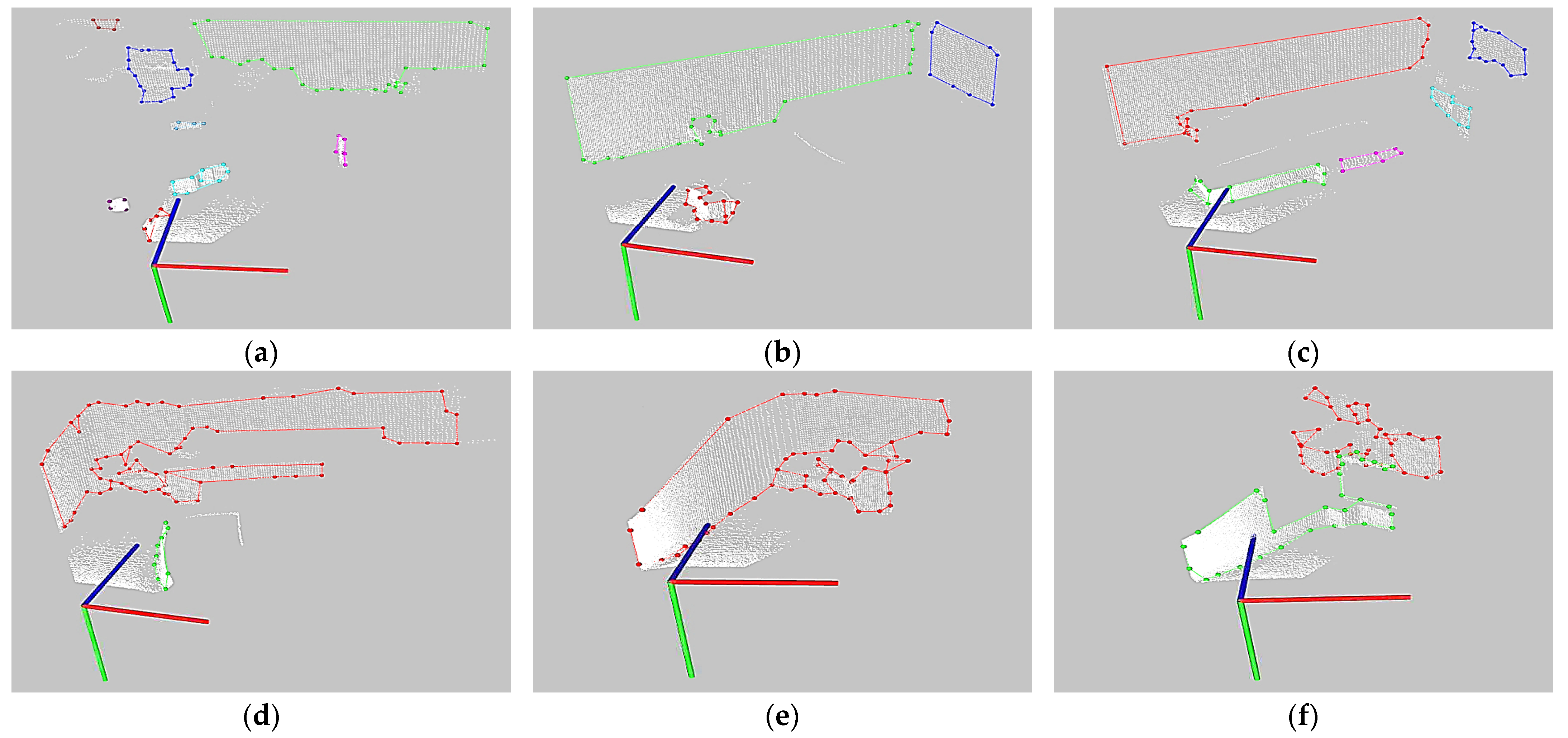
Table 4. 3D object extraction performance.
No.Input
Image
No. of Points in Point CloudNo. of NodesNo. of
Connections
No. of ClustersMin Distance
between Nodes
Max Distance between NodesTime [ms]
1Figure 14a8586778080.100 m2.430 m32.7
2Figure 14b11,647484930.100 m3.210 m27.6
3Figure 14c10,455616750.100 m3.180 m34.6
4Figure 14d10,802808620.102 m1.575 m35.6
5Figure 14e13,948546010.102 m1.217 m32.1
6Figure 14f14,094707620.100 m0.560 m30.0
Frame Rate:Mean = 1   s 32.1   m s = 31.15 fps; Min = 1   s 35.6   m s = 28.09 fps; Max = 1   s 27.6   m s = 36.23 fps
Table 5. Parameter settings for 2D–3D combination method.
ParameterValueDefinition
thetaTh10°DBSCAN clustering rotation threshold
dEps0.10 m (step 2) 0.15 m (step 4)DBSCAN clustering minimum search radius
minObj2DBSCAN clustering minimum number of objects
maxIteration1.5 nRANSAC maximum iteration. n is the number of sample data
inliersTh0.10 m (step 3, 4)RANSAC inlier threshold
Table 6. Computational costs of real-time experiments.
PC Controller
No.NetworkData Transmission Time [ms]
Mean of 50+ Data
Mean [ms]2D SLAM and 2D–3D Combination [ms]
Mean of 50+ Data
Mean [ms]Data Size [KB]
Mean of 50+ Data
Mean [KB]
1Wi-Fi to LoRa27327493980.7270.734
2266920.740
32771060.735
4272960.718
52801060.752
6LoRa57062589990.4630.471
77031060.472
86181020.474
9577980.471
106591030.475
11Wi-Fi17181091120.9260.932
12231080.928
13161160.936
14171090.914
15181180.936
Mobile Robot
HardwareSampling RateAlgorithmEncodingTotal
2D Data2D LiDAR25 fps (40 ms)3× Downsampling: 10 ms5 ms55 ms
3D DataLiDAR Camera30 fps (33 ms)Simplified FastGNG: 32.1 ms (mean)10 ms75.1 ms
Total Computational Cost
Wi-Fi to LoRa274 ms + 98 ms + 75.1 ms = 447.1 ms (2.24 Hz)
LoRa625 ms + 99 ms + 75.1 ms = 799.1 ms (1.25 Hz) (main target)
Wi-Fi18 ms + 112 ms + 75.1 ms = 205.1 ms (4.88 Hz)
Disclaimer/Publisher’s Note: The statements, opinions and data contained in all publications are solely those of the individual author(s) and contributor(s) and not of MDPI and/or the editor(s). MDPI and/or the editor(s) disclaim responsibility for any injury to people or property resulting from any ideas, methods, instructions or products referred to in the content.

