Neural Network Mapping of Industrial Robots’ Task Times for Real-Time Process Optimization

Abstract

The ability to predict the maximal performance of an industrial robot executing non-deterministic tasks can improve process productivity through time-based planning and scheduling strategies. These strategies require the configuration and the comparison of a large number of tasks in real time for making a decision; therefore, an efficient task execution time estimation method is required. In this work, we propose the use of neural network models to approximate the task time function of a generic multi-DOF robot; the models are trained using data obtained from sophisticated motion planning algorithms that optimize the shape of the trajectory and the executed motion law, taking into account the kinematic and dynamic model of the robot. For scheduling purposes, we propose to evaluate only the neural network models, thus confining the online use of the motion planning software to the full definition of the actually scheduled task. The proposed neural network model presents a uniform interface and an implementation procedure that is easily adaptable to generic robots and tasks. The paper’s results show that the models are accurate and more efficient than the full planning pipeline, having evaluation times compatible with real-time process optimization.

1. Introduction

The throughput of an industrial application using one or more robots with a fixed base depends on the cycle time of the movement executed by the robot to perform the task. Therefore, the choice of movements with the shortest cycle time increases the number of operations in the reference time, enhancing the robot application’s productivity.

The cycle time of pick and place operations depends on several aspects, such as the kinematic structure of the robot, its inertial characteristics, and the properties of its actuation and transmission systems, which all concur to limit the maximal achievable velocities and accelerations; an important role is played also by the trajectory’s shape, by the motion profile on it, and by its position inside the robot’s working volume.

The choice of the robot’s movement with the shortest cycle time is straightforward for fixed pick and place positions. In this case, an offline procedure based on the robot’s software environment can be used. In more complex cases, however, the pick and place positions are not known in advance, and moreover might be non-stationary; for such cases, then, three types of pick and place tasks may be distinguished: (a) tasks on fixed pick and place targets, which are known in advance and do not change in time; (b) stationary pick and place tasks, in which the targets do not move while the robot is performing its operations but which are dynamically reconfigured and a priori unknown; (c) on-the-fly pick and place tasks, in which the targets are not known in advance and also move while the robot operates on them.

Tasks of type (b) and (c) occur, e.g., in modular multi-robot work cells where a series of robots operates on a transportation system that intermittently or continuously conveys the items to be processed. Each robot, which, as exemplified in Figure 1, must sort, manipulate, and rearrange items randomly loaded onto the transportation system, operates therefore under time constraints in a time-varying and non-deterministic environment.

In this kind of application, the definition of the robot’s movement with the shortest cycle time is a complex process, requiring an optimization strategy based on the changing scenario that the robot is presented with and on the robot’s characteristics. For stationary pick and place positions, the process optimization problem concerns the sequencing of the tasks. For on-the-fly manipulation, an additional optimization problem, i.e., the computation of the best position at which the robot intercepts its moving target, must be preliminarily solved.

Additional problems that must be solved after a task has been scheduled are first the geometric motion planning, which defines the shape of the trajectory to be executed by the robot, and then the generation of the motion law along the geometric path.

The load balancing and task assignment problems for assembly lines and multi-robot cells have been treated in the current literature from an operational research perspective. In [1,2,3,4,5], the actual capabilities of the robot are indeed expressed in terms of its cycle times, which are considered not as a function of the properties of the robot and of the tasks but either as a random variable [1], as an average value to which other independent contributions (such as waiting times) might added [2,3], or as a single fixed value [4,5].

The intercept problem both for manipulators and for mobile robots, in which the precise estimation of the task times becomes a focal point, emerges in a variety of applications and has been treated according to several approaches. In [6], a Particle Swarm Optimization method is proposed for a coal gangue processing plant served by a conveyor and by Cartesian robots; [7] discusses a heuristic algorithm for the real-time solution of the rendezvous problem between unmanned aerial vehicles operating in a leader-follower configuration. In [8], the intercept problem for objects moving on a conveyor belt was solved online within a bisection search algorithm, which requires the evaluation of the task times of a robot moving with trapezoidal velocity profiles. A similar concept was described earlier in [9], in which the traveling time curve of the robot is iteratively approximated online; the possibility of recomputing the intercept position in case of variations of the moving target’s trajectory is also included. In [10], target tracking and collision avoidance with moving obstacles are jointly treated using a Model Predictive Control framework in which neural networks are used to implement the models of the robot and of the obstacle dynamics.

These works are characterized by the online definition of the task time curves of the robot, or, as in [10], by a reactive approach that does not require the evaluation of the task time curve. Alternative approaches are instead based on the pre-evaluation of the robot task times. This general idea is discussed in [11], in which the execution times are obtained from the Reflexxes Motion Library [12]; an early example of an analogous concept can be found in [13], in which experimental data collected from the actual use of the robot are arranged in a simple task time lookup table. More recently, also [14] solved the optimal intercept problem for pick and place tasks on a rotating table using a two-dimensional task time table adapted to the radial geometry of the problem; the motion planning of each trajectory is performed using the commercial software that accompanies the robot controller. In a similar vein, [15] constructs a task time table needed for pick and place operations on a moving conveyor. In that work, the dependence of the cycle time function on the manipulator’s specific properties is highlighted. The procedure for the determination of the cycle time data is not described, as reliance is again placed on the Reflexxes Motion Library. The authors assume that the velocity of the conveyor is fixed, and only a rectangular portion of the workspace of the robot is considered. In [16], the concept of a task-dependent map emerges in relation not to the execution times but rather to the energy consumption associated with each operation. The resulting energy map is three-dimensional and expressed in a cylindrical system.

To maximize the throughput of the robot, it is necessary to minimize the execution times of its tasks; hence, the minimization of the travel time along a given geometric path under constraints determined by the physical properties of the robot has received considerable attention and has been treated successfully according to a variety of methods. The algorithm described by Bobrow et al. [17] constructs time-optimal trajectories characterized by $C^0$ velocities using a numerical integration approach. Further refinements were proposed by [18]. A similar result is obtained through an algorithm based on reachability analysis developed in [19], while other commonly applied approaches are based on convex optimization [20]. These methods differ in terms of ease of implementation and computational cost; a further significant difference lies in their ability to include more or less straightforwardly third-order constraints whose main purpose is the limitation of the motion jerk. Such constraints were included in an exact but cumbersome way within the numerical integration approach [21], whereas methods based on convex optimization were shown to be able to consider motion jerk constraints rather straightforwardly, though not exactly [22,23]. A commonality of these works is that the geometric path is considered a given; the problem of generating suitable geometric trajectories remains therefore out of their scope. The geometric path planning, indeed, is more application specific and thus less amenable to be treated in a standard way. Different strategies and ideas, a review of which can be found in [24], can be specialized for use in diverse fields such as race driver modeling [25], routing of mobile robots for agricultural applications [26], CNC milling [27,28], and fixed-based robots operating in cluttered environments [29].

The current literature reveals the following gaps:

• the scheduling, the optimal intercept computation, and the trajectory execution time minimization are treated in isolation, without considering the interdependencies between them;
• the scheduling algorithms often do not consider accurately that different tasks are associated with different execution times;
• the cycle or task time maps are developed without a focus on the optimal (as opposed to feasible) times;
• the cycle time maps or tables cover only a portion of the useful workspace of the manipulator and appear tailored to a specific application;
• the methods employed for the generation of the cycle time maps are known to scale poorly to problems featuring a high number of degrees of freedom.

To address these gaps, this work proposes a mapping of the robot’s task time using neural networks. The use of a neural network model results in a task time map covering the entire workspace of the robot and presenting a uniform software interface.

For the collection of the data needed to train the map, the authors take into account all the aspects that determine the task time, namely the kinematics and dynamics of the manipulator, the geometric motion planning, and the task time optimization. This paper illustrates therefore the geometric planning and task time minimization procedures that enable the generation of the task time data directly from simulations. Since these software modules are based on the mechanical model of the robot, its properties and limitations are reflected in the generated training dataset and therefore also in the trained task time map. The proposed approach remains applicable also in cases in which the software modules for the generation of appropriate datasets are not available, since the neural network model can also be trained with experimental data, whose collection is however more expensive and time consuming.

The geometric planning and task time minimization are relatively demanding procedures, which should be invoked sparingly during real-time computations. The evaluation of the task time map, on the contrary, is orders of magnitude faster, making the map itself an essential component of the real-time optimizing scheduler that solves the intercept problem and defines the robot’s tasks. In particular, since the pick and place targets are moving, the task has to be defined in a useful time window, before the targets move past the robot’s reach. The task time map is therefore used to speed up these computations.

The main contributions of the article are:

• the development of a systematic architecture for the representation of the task time maps as neural networks;
• the illustration of a computational procedure for the generation of the dataset needed to train the task time models;
• the demonstration of the use of the task time maps to solve the optimal intercept problem in an industrial application case.

The paper is structured as follows. An outline of the problem and an overview of the proposed solution are first presented. The proposed methodologies and the necessary algorithms for the creation of the task time map are then illustrated; their implementation in relation to a full-featured case study is then shown. The results concerning two applications of the task time map are finally discussed: one related to pick and place operations on items carried by a conveyor that advances intermittently, the other related to on-the-fly manipulation of objects moving on a conveyor that advances continuously and with slowly adjustable speed.

2. Methods

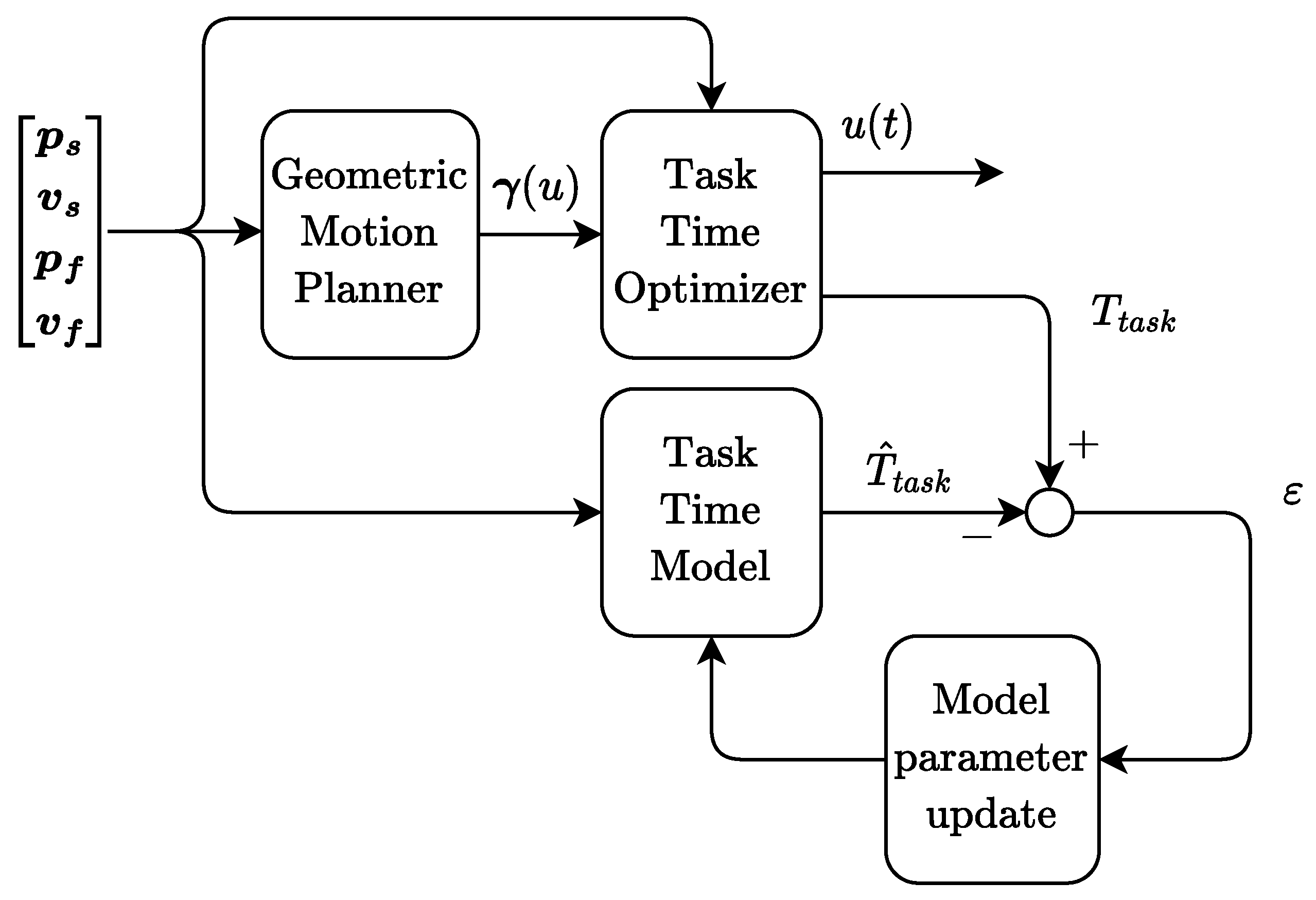
2.1. Problem Statement and Solution Outline

The paper denotes as a task or job a configurable elementary operation that can be performed by the robot. Chaining multiple elementary tasks results in a composite task; a task that is executed in a repeating pattern constitutes a work cycle. The scheduler is a proper software algorithm that selects and configures the next job assigned to the robot among all the possibilities. Several scheduling strategies that aim at the maximization of the throughput of the system, such as the Shortest Job Next or the Highest Response Ratio Next rules, require the knowledge of the execution times associated with each of the possible tasks. To implement this kind of scheduler, a map that associates the jobs that can be executed inside the workspace of the robot to their minimal execution time is then needed. If required by the application, the map can be used by the scheduler also for solving the optimal intercept problem, which likewise is governed by the task time function.

An elementary task is defined by a geometric path and by the motion profile on it. The geometric path $\gamma :[u_{lb},u_{ub}]\to \Omega \subset {\mathbb{R}}^{n_f}$ is a function mapping a real number belonging to the interval $[u_{lb},u_{ub}]$ into the $n_f$-dimensional robot’s task space $\Omega$. A point in $\Omega$ is denoted as $\mathit{p}$; $\mathit{v}$ and $\mathit{a}$ denote likewise velocities and accelerations.

The motion profile on the geometric path is representable as a function $u:[t_s,t_f]\to [u_{lb},u_{ub}]$, where $[t_s,t_f]$ is the time interval in which the motion is executed. Therefore, to define a task, two issues arise, namely the definition of the function $\gamma$ and of the function u. Once these two functions have been defined, the task execution time $T_{task}=t_f-t_s$ is also defined. In robotic applications, the definition of the geometric path and of the motion profile is typically decoupled. The geometric path is commonly defined by the Geometric Trajectory Planner (GTP); the motion profile can be on the other hand defined by a separate software module, the Task Time Optimizer (TTO). The GTP and the TTO can be thought of as two higher-order functions, denoted each as G and H, that accept a certain number of inputs and have as output, respectively, functions $\gamma$ and u. Concerning the GTP module, it can be said that its implementation is highly application-specific. In general, however, the geometric definition of a task requires a set of position, velocity, and acceleration boundary conditions plus a set of further configuration parameters; the output is a geometric path. Denoting as ${\mathit{c}}_G$ the further configuration parameters, we can write the following:

$$\begin{array}{c}\hfill \gamma \leftarrow G({\mathit{c}}_G,{\mathit{p}}_s,{\mathit{v}}_s,{\mathit{a}}_s,{\mathit{p}}_f,{\mathit{v}}_f,{\mathit{a}}_f).\end{array}$$

(1)

As already stated in the introduction, standard algorithms for the TTO exist; irrespectively of the implementation details, these algorithms can be assumed to take the form of a higher-order function:

$$\begin{array}{c}\hfill u\leftarrow H({\mathit{c}}_H,\gamma ,{\mathit{p}}_s,{\mathit{v}}_s,{\mathit{a}}_s,{\mathit{p}}_f,{\mathit{v}}_f,{\mathit{a}}_f),\end{array}$$

(2)

where ${\mathit{c}}_H$ are configuration parameters of the task time optimizer. The output of H, usually determined through an optimization procedure that takes into consideration the properties of the robot, is the motion profile u.

The functions G and H must be such that the following equalities hold:

$$\begin{array}{ccc}\hfill \gamma \left(u\left(t_s\right)\right)& =& {\mathit{p}}_s\hfill \end{array}$$

(3)

$$\begin{array}{ccc}\hfill \dot{\gamma }\left(u\left(t_s\right)\right)& =& {\mathit{v}}_s\hfill \end{array}$$

(4)

$$\begin{array}{ccc}\hfill \ddot{\gamma }\left(u\left(t_s\right)\right)& =& {\mathit{a}}_s\hfill \end{array}$$

(5)

$$\begin{array}{ccc}\hfill \gamma \left(u\left(t_f\right)\right)& =& {\mathit{p}}_f\hfill \end{array}$$

(6)

$$\begin{array}{ccc}\hfill \dot{\gamma }\left(u\left(t_f\right)\right)& =& {\mathit{v}}_f\hfill \end{array}$$

(7)

$$\begin{array}{ccc}\hfill \ddot{\gamma }\left(u\left(t_f\right)\right)& =& {\mathit{a}}_f.\hfill \end{array}$$

(8)

In light of assignments (1) and (2), it can be said that each elementary task is ultimately defined by the boundary conditions ${\mathit{p}}_s$, ${\mathit{v}}_s$, ${\mathit{a}}_s$, ${\mathit{p}}_f$, ${\mathit{v}}_f$, ${\mathit{a}}_f$ and by the parameters ${\mathit{c}}_G$, ${\mathit{c}}_H$. Therefore, the task execution time $T_{task}$ is also a function of these same parameters. It is clear that the evaluation of $T_{task}$ is an expensive procedure that requires the application of G and H.

In general terms, we define as the task time map ${\widehat{T}}_{task}$ a function of the form:

$$\begin{array}{c}\hfill {\widehat{T}}_{task}={\widehat{T}}_{task}({\mathit{c}}_G,{\mathit{c}}_H,{\mathit{p}}_s,{\mathit{v}}_s,{\mathit{a}}_s,{\mathit{p}}_f,{\mathit{v}}_f,{\mathit{a}}_f)\end{array}$$

(9)

whose output nominally matches $T_{task}$.

Without loss of generality, this work considers applications where the configuration parameters are embedded into the GTP and TTO implementations. Additionally, since for motion control purposes the enforcement of acceleration boundary conditions is not strictly required, in the following discussion we do not consider them as input parameters. As a result of these assumptions, which still allow us to deal with most industrial cases of any practical interest, the task time map will assume the form: ${\widehat{T}}_{task}={\widehat{T}}_{task}({\mathit{p}}_s,{\mathit{v}}_s,{\mathit{p}}_f,{\mathit{v}}_f)$.

The paper presents the development of the task time map as a neural network model and the definition of a strategy for generating suitable training datasets. Moreover, the paper presents how the map is helpful for efficiently solving the optimal intercept problem. Further uses, discussed conceptually in this article, are related to implementing efficient scheduling algorithms usable in real-time software applications.

To precisely define the optimal intercept problem, the authors assume that the motion of the target (i.e., of the object to be intercepted by the robot) is a known curve in $\Omega$ of the form ${\gamma }_{tgt}\left(t\right)$. In addition, the time derivatives of ${\gamma }_{tgt}$ are known. The solution of the following equation formally defines the optimal intercept problem:

$$\begin{array}{c}\hfill T_{task}({\mathit{p}}_s,{\mathit{v}}_s,{\gamma }_{tgt}\left(t\right),{\dot{\gamma }}_{tgt}\left(t\right))=t.\end{array}$$

(10)

The quantities ${\mathit{p}}_s$ and ${\mathit{v}}_s$ are determined by the current state of the robot. Equation (10) is therefore univariate; its solution yields the time $t_{intercept}$ and position ${\gamma }_{tgt}\left(t_{intercept}\right)$ at which the robot can intercept the target. As the solution is in general not unique, the one characterized by the minimal $t_{intercept}$ should be selected.

In order to solve the optimal intercept Equation (10), numerical solving is required, which can involve a large number of iterations. However, substituting $T_{task}$ with ${\widehat{T}}_{task}$ can significantly reduce the computation time. This approach meets the soft real-time constraints, which are necessary because the environment in which the robot operates is not stationary.

Within a complete software stack for a practical robotic application, the GTP and TTO modules should be reasonably efficient, as they are used once for each scheduled task to fully define it; the task time map ${\widehat{T}}_{task}$ on the other hand needs to be not only accurate but also much faster than the direct determination of $T_{task}$ because both the solution of the optimal intercept and the task scheduling require its frequent evaluation.

The scheduling and planning operations are represented graphically in Figure 2 according to the above discussion, though with an eye towards the industrial case of interest, which is a pick and place line with conveyors moving with quasi-statically adjustable velocity.

The scheduler requires as inputs the current position ${\mathit{p}}_{\mathit{rbt}}$ and velocity ${\mathit{v}}_{\mathit{rbt}}$ of the manipulator’s end effector and a list of current positions ${\mathit{p}}_{\mathit{tgt},\mathbf{1}}\dots {\mathit{p}}_{\mathit{tgt},\mathit{n}}$ and velocities ${\mathit{v}}_{\mathit{tgt},\mathbf{1}}\dots {\mathit{v}}_{\mathit{tgt},\mathit{n}}$ of the pick and place targets, which are detected, e.g., by a vision system.

The scheduler performs two operations according to the information provided by the task time map. First, if the targets are moving, it computes the positions at which the robot should intercept them. Subsequently, it identifies the target that should be processed next among all the possibilities.

The outputs of these operations are the position and velocity boundary conditions of the trajectory needed to perform the pick or place task: the scheduler sets the starting position and velocity ${\mathit{p}}_{\mathit{s}}$ and ${\mathit{v}}_{\mathit{s}}$ equal to the current position and velocity of the robot; the final position and velocity ${\mathit{p}}_{\mathit{f}}$ and ${\mathit{v}}_{\mathit{f}}$ are instead defined according to the solution of the intercept problem of the chosen target. Once ${\mathit{p}}_{\mathit{s}}$, ${\mathit{v}}_{\mathit{s}}$, ${\mathit{p}}_{\mathit{f}}$, and ${\mathit{v}}_{\mathit{f}}$ have been defined, the geometric planning can be performed, yielding a parametric curve $\gamma \left(u\right)$. This curve defines the geometry of the trajectory, but not the motion law on it, whose generation is demanded instead to the task optimization routine, which outputs the time reparametrization $\gamma \left(u\right(t\left)\right)$ and in suborder the actual task execution time $T_{task}$.

The geometric trajectory planning is strongly tied to the type of application and can be developed only in relation to it. This work proposes a geometric planning approach suitable for pick and place applications where the manipulator can either perform pick and place operations on stationary targets or also follow non-stationary picking and placing positions, which move along a given direction. This problem arises when the manipulator is used to pick and place the payload from and onto moving conveyors. We note that the implementation of the Geometric Trajectory Planner defines classes of parametrized tasks, which, in our case, there are two: stationary and on-the-fly pick and place tasks.

In Figure 3, the input–output relationships between the environment, the scheduler, the GTP, and the TTO are illustrated in accordance with the description above.

Here, it can be seen clearly that the task time estimation needed by the scheduler is provided by the task time map, which ideally should coincide with the function that associates the tasks with their execution times. The exact evaluation of the task time function using the GTP and the TTO is however rather expensive; therefore, for scheduling purposes, the task time map is used in their stead to efficiently determine the task times.

To generate the map, a representative sample of the task times must be collected. The task time data can be obtained from the robot’s tasks offline simulation, performed using the GTP and the TTO. The training data can also be obtained by experimental tests using the robot for the given payload, for the given boundary conditions, and for a set of trajectories whose starting and ending points thoroughly cover the working space. In this case, the cost and the time for collecting the data can be high, but the need for the development of the GTP and TTO is removed, as reliance can be placed on the robot’s accompanying software. In addition, in this case, the proposed approach based on the creation of the task time map as a deep learning model remains still valid. Within this work, the authors focus on the computational approach, notwithstanding the fact that the experimental generation of the needed dataset remains a possibility.

The proposed approach is useful for applications that involve robots and movements with several degrees of freedom, where each task can be configured according to a large number of parameters, i.e., the initial and final positions and velocities of the robot. In these cases, the simpler table-based lookup approaches do not exhibit either a uniform interface or a general implementation procedure and are not suitable for the description of the task time map, not only because of the irregular geometry of the robot’s workspace but also because of the large dimensionality of the problem. The representation of the task time map through the use of artificial neural networks overcomes the difficulties associated with more traditional table-based lookup structures: in addition to being inherently mesh-free and adaptable to the workspace geometry, it also offers the advantages both of a standard query interface and of a generation methodology that remains independent from the specific characteristics of the robot and of the application.

The paper also address the fact that an accurate and reliable model can be generated only from task time data that reflect:

• the kinematic and dynamic properties of the robot;
• the parameters of the actuators and transmission systems;
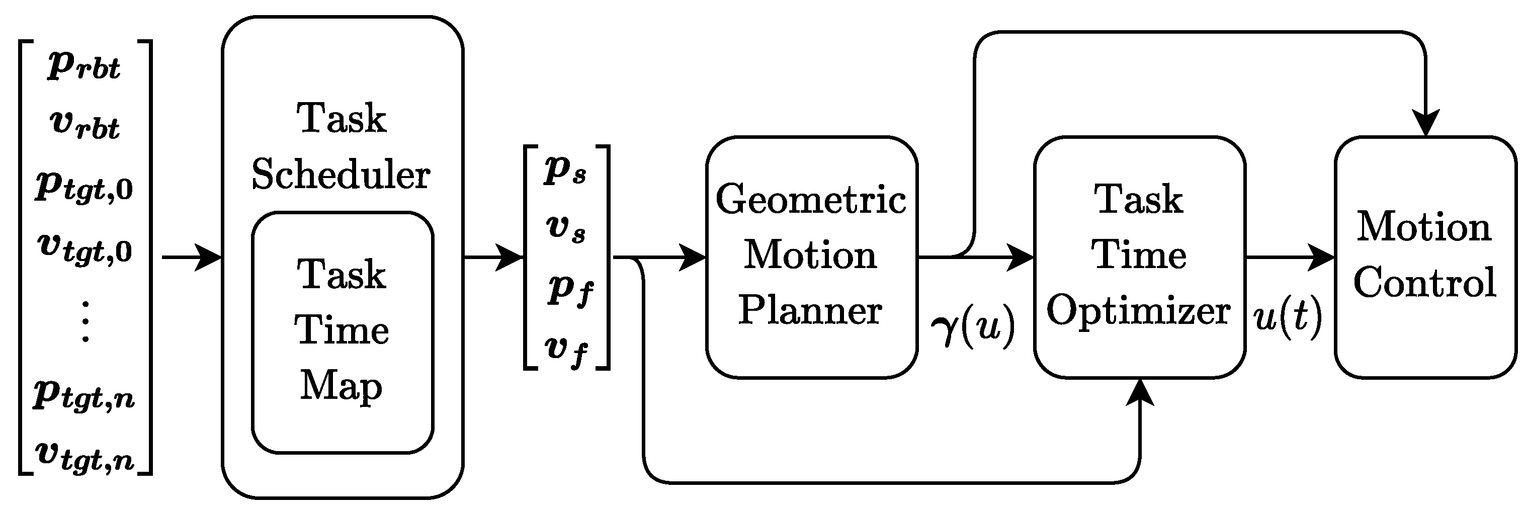
• the behavior of the Geometric Planning Module;
• the behavior of the Task Time Optimizer.

This work proposes therefore a systematic procedure that includes the following steps:

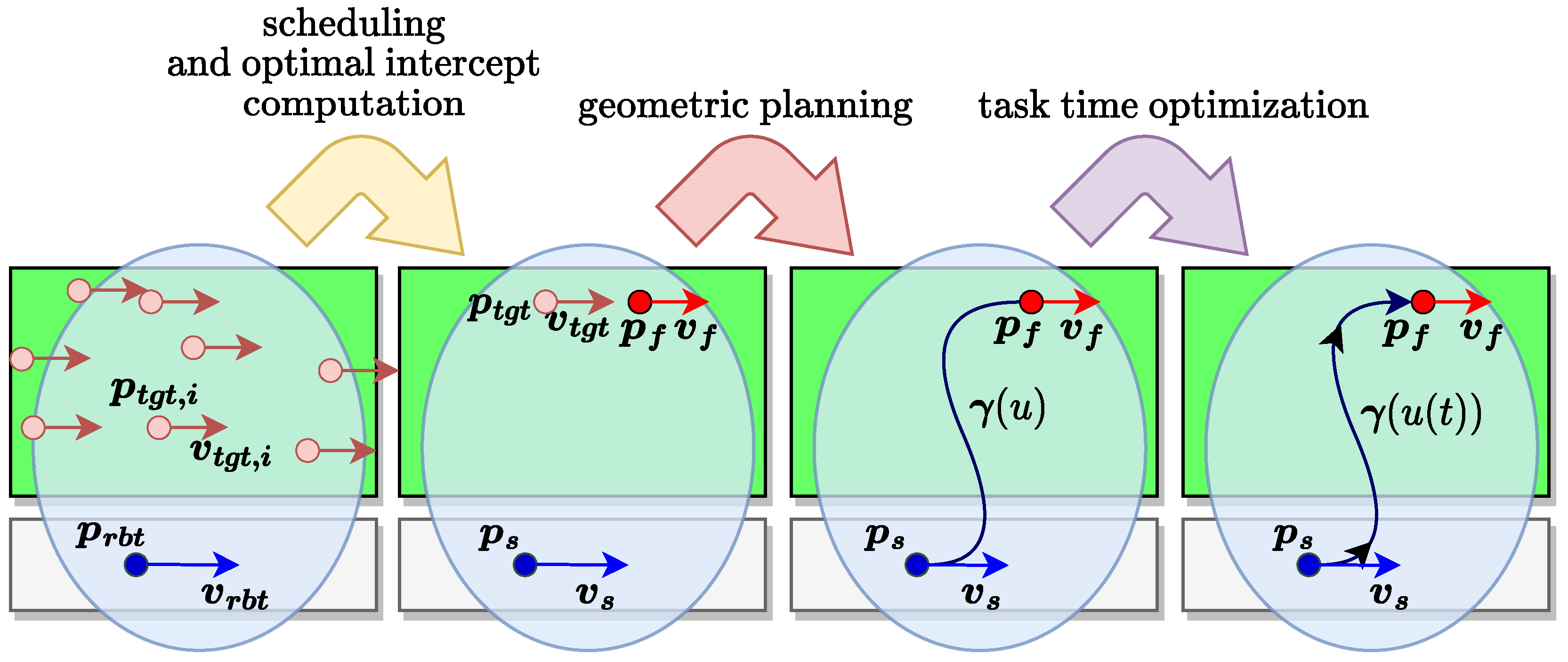
• the parametrization of the tasks to be executed by the robot using the GTP;
• the offline generation of a dataset of optimal execution times using the TTO;
• the generation, using deep learning models, of an accurate and efficiently queryable map of the optimal task times over the entire workspace of the robot.

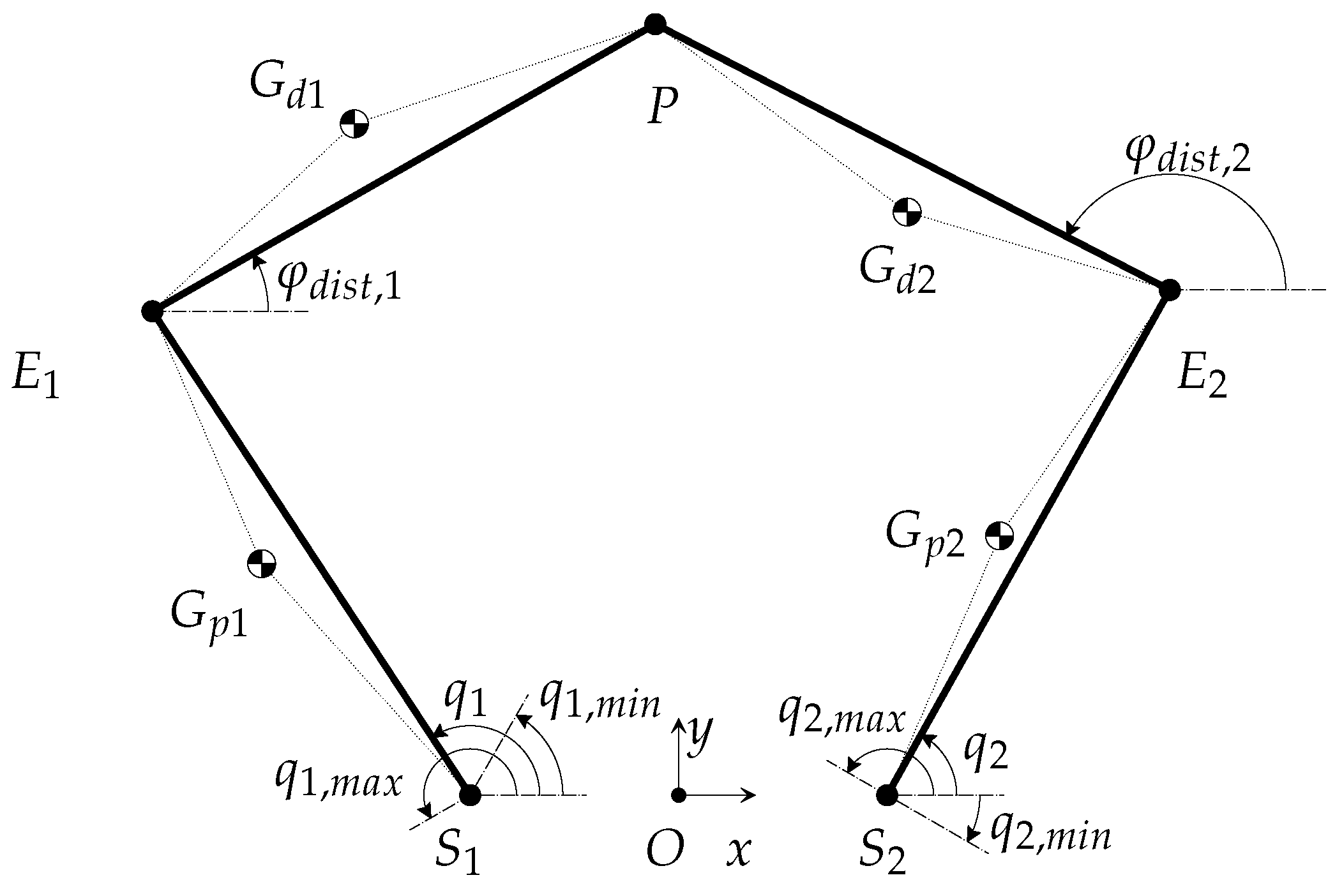
2.2. Geometric Trajectory Planning

The geometric trajectory planner accepts as inputs the configuration parameters of the path’s geometry. These are the initial and final configurations of the manipulator, expressed as position and velocity boundary conditions.

The geometric planner should generate as its output a parametric curve $\gamma \left(u\right)$, with parameter u belonging to an interval $\left[u_{lb},u_{ub}\right]$. In this paper, curves having $C^2$ continuity are considered in order to avoid points along the trajectory necessarily characterized by unbounded motion jerk. Clearly, the curves should also belong entirely to the workspace of the robot and should not cross any singular configuration.

How to efficiently achieve these goals depends on the properties of the robot, which determine the shape both of the workspace and of the singular loci. Additional requirements are obstacle avoidance and specific shape characteristics, which furthermore depend on the robot’s environment and on the type of task. Therefore, we postpone the detailed description of our Geometric Trajectory Planner implementation to the application case presented in Section 3.

2.3. Task Time Optimization

As already stated in the introduction, several methodologies are well described in the literature for the implementation of the Task Time Optimizer (TTO) as a constrained optimization process that accepts as inputs a geometric description of the trajectory and higher-order boundary conditions. The constraints are computed according to:

• the actual performances of the actuation drives and of the transmissions;
• the model of the mechanical dynamics of the manipulator;
• the properties of the payload.

The main output of the TTO is the motion along the geometric path that minimizes the travel time while remaining compatible with the performances of the robot. The minimal execution time can also be obtained as a further output of the TTO.

Let $\mathit{q}$ be the parameters describing the robot pose in the joint space, and let the dynamics of the robot be expressed in the form:

$$\begin{array}{c}\hfill \mathit{M}\left(\mathit{q}\right)\ddot{\mathit{q}}+\mathit{C}(\mathit{q},\dot{\mathit{q}})\dot{\mathit{q}}+\nabla U\left(\mathit{q}\right)=\mathit{\tau },\end{array}$$

(11)

where $\mathit{M}$ is the mass matrix, $\mathit{C}$ is the Coriolis matrix, U is the potential energy, and $\mathit{\tau }$ are the torques exerted at the joints.

The task time optimization typically uses a robot’s dynamics formulation that neglects the compliance of the transmission units and of the links; this simplification can be considered acceptable whenever these aspects have been appropriately considered during the design stage of the robot, as shown, e.g., in [30,31].

Using Lagrange equations, it can be straightforwardly shown that $\mathit{C}(\mathit{q},\dot{\mathit{q}})$ is homogeneous with respect to $\dot{\mathit{q}}$:

$$\mathit{C}(\mathit{q},\alpha \dot{\mathit{q}})=\alpha \mathit{C}(\mathit{q},\dot{\mathit{q}}).$$

(12)

Even though $\gamma \left(u\right)$ is typically formulated in the task space, the robot’s inverse kinematic relationships can be applied to express the same motion in the joint space. The path-projected dynamic equations can be then expressed in the form:

$$\begin{array}{c}\hfill m_i\left(u\right)\ddot{u}+c_i\left(u\right){\dot{u}}^2+g_i\left(u\right)={\tau }_i,\end{array}$$

(13)

where $m_i$, $c_i$, $g_i$ are each the $i^{th}$ elements of the vectors:

$$\begin{array}{ccc}\hfill \mathit{m}\left(u\right)& =& \mathit{M}(\mathit{q}\left(u\right)){\mathit{q}}^{\prime }\left(u\right)\hfill \end{array}$$

(14)

$$\begin{array}{ccc}\hfill \mathit{c}\left(u\right)& =& \mathit{M}(\mathit{q}\left(u\right)){\mathit{q}}^{\prime \prime }\left(u\right)+\mathit{C}(\mathit{q}\left(u\right),{\mathit{q}}^{\prime }\left(u\right)){\mathit{q}}^{\prime }\left(u\right)\hfill \end{array}$$

(15)

$$\begin{array}{ccc}\hfill \mathit{g}\left(u\right)& =& \nabla U\left(\mathit{q}\right(u\left)\right).\hfill \end{array}$$

(16)

Each power drive system (i.e., the driver-motor unit) actuating the robot is characterized by a maximum admissible torque ${\tau }_{pds,max,i}$, by a rated torque ${\tau }_{pds,rated,i}$, by a maximum velocity ${\omega }_{pds,max,i}$, and by an inertia ${J_m}_{,i}$, all expressed at the motor shaft. Additionally, the transmission system is characterized by a reduction ratio $i_{t,i}$, by an efficiency ${\eta }_{t,i}$, and by an inertia ${J_t}_{,i}$, typically expressed with respect to the input shaft. All these parameters are fundamental in determining the minimal execution time of a given trajectory; although they are considered as a given as far as the TTO is concerned, they must be carefully selected during the design phase of the manipulator. A procedure for the proper configuration of the power drive systems and transmissions is illustrated in [32].

The inertial properties of motor and transmission are easily projected on the output shaft and thus accounted for within $\mathit{M}$.

Assuming a continuative use, the following constraints can be conservatively enforced:

$$\begin{array}{c}\hfill \left|m_i\left(u\right)\ddot{u}\left(u\right)+c_i\left(u\right){\dot{u}}^2\left(u\right)+g_i\left(u\right)\right|\le {\eta }_{t,i}{i}_{t,i}{\tau }_{pds,rated,i}.\end{array}$$

(17)

In this way, it can be ensured that the constraints on the RMS torque (and therefore also on the peak torque) are satisfied. The constraints on the maximum rotational speed of the actuators can moreover be written as:

$$\begin{array}{c}\hfill -{\displaystyle \frac{{\omega }_{pds,max,i}}{i_{t,i}}}\le {q_i}^{\prime }\left(u\right)\dot{u}\le {\displaystyle \frac{{\omega }_{pds,max,i}}{i_{t,i}}}.\end{array}$$

(18)

As suggested in [20], the following change of variables is introduced: let

$$\begin{array}{c}\hfill x\left(u\right)={\dot{u}}^2\left(t\left(u\right)\right);\end{array}$$

(19)

then:

$$\begin{array}{cc}\hfill x^{\prime }\left(u\right)& =2\ddot{u}\left(t\right).\end{array}$$

(20)

Constraints equivalent to those of Inequality (18) can be written as:

$$\begin{array}{c}\hfill {{q_i}^{\prime }}^2\left(u\right)x\left(u\right)\le {\left({\displaystyle \frac{{\omega }_{pds,max,i}}{i_{t,i}}}\right)}^2\end{array}$$

(21)

while Inequality (17) can be rewritten as

$$\begin{array}{c}\hfill \left|{\displaystyle \frac{m_i\left(u\right)}{2}}{x}^{\prime }\left(u\right)+c_i\left(u\right)x\left(u\right)+g_i\left(u\right)\right|\le {\eta }_{t,i}{i}_{t,i}{\tau }_{pds,rated,i}.\end{array}$$

(22)

The optimal function ${\dot{u}}_{opt}\left(u\right)=\sqrt{x_{opt}\left(u\right)}$ is commonly intended as the one minimizing the total traveling or task time $T_{task}$, itself expressible as:

$$\begin{array}{c}\hfill T_{task}={\int }_{u_{lb}}^{u_{ub}}{\displaystyle \frac{\mathrm{d}u}{\sqrt{x\left(u\right)}}}.\end{array}$$

(23)

The optimization problem described above, in which $T_{task}$ is the cost function, needs to be discretized in order to be solved. The constraints are therefore enforced not on the entire interval of definition of the parameter u but only on a finite number of values $u_j$, with $j=0,1,\dots ,m-1$. To obtain a finite number of decision variables $\mathit{x}$, the function $x\left(u\right)$ is assumed to be of the form:

$$\begin{array}{ccc}\hfill x\left(u\right)& =& \mathit{N}{\left(u\right)}^T\mathit{x}\hfill \end{array}$$

(24)

$$\begin{array}{ccc}\hfill x^{\prime }\left(u\right)& =& {\mathit{N}}^{\prime }{\left(u\right)}^T\mathit{x},\hfill \end{array}$$

(25)

where $\mathit{N}\left(u\right)$ is a suitable vector-valued shape function. The shape function can be isolated, leading to the reformulation of the $j^{th}$ constraint inequalities as:

$$\begin{array}{cc}\hfill {\left({\displaystyle \frac{m_i\left(u_j\right)}{2}}{\mathit{N}}^{\prime }\left(u_j\right)+c_i\left(u_j\right)\mathit{N}\left(u_j\right)\right)}^{\top }\mathit{x}\le & {\eta }_{t,i}{i}_{t,i}{\tau }_{pds,rated,i}-g_i\left(u_j\right)\end{array}$$

(26)

$$\begin{array}{cc}\hfill {\left({\displaystyle \frac{m_i\left(u_j\right)}{2}}{\mathit{N}}^{\prime }\left(u_j\right)+c_i\left(u_j\right)\mathit{N}\left(u_j\right)\right)}^{\top }\mathit{x}\ge & -{\eta }_{t,i}{i}_{t,i}{\tau }_{pds,rated,i}-g_i\left(u_j\right)\end{array}$$

(27)

$$\begin{array}{c}\hfill {\left({q_i}^{\prime }\left(u_j\right)\right)}^2\mathit{N}{\left(u_j\right)}^{\top }\mathit{x}\le {\omega }_{pds,max,i}^2,\end{array}$$

(28)

which are linear with respect to the decision variables $\mathit{x}$. The cost function $T_{task}$ can be approximated as follows:

$$\begin{array}{ccc}\hfill {\tilde{T}}_{task}& =& \sum _{k=1}^n{\displaystyle \frac{\Delta u}{\sqrt{\mathit{N}{\left(u_k\right)}^{\top }\mathit{x}}}},\hfill \end{array}$$

(29)

leading to the optimization problem:

$$\begin{array}{c}\hfill {\tilde{T}}_{task,min}=\underset{\mathit{x}}{min}{\tilde{T}}_{task}\mathrm{under}\mathrm{constraints}\left(26\right)–\left(28\right).\end{array}$$

(30)

As ${\tilde{T}}_{task}$ is convex with respect to $\mathit{x}$, the solution of the time reparametrization problem for a given trajectory can be found using appropriate convex optimization solvers. On the other hand, the structure of the problem and of the constraints suggests the setup of a different optimization problem, namely:

$$\begin{array}{ccc}\hfill {\Phi }_{}\left(\mathit{x}\right)& =& \left[\begin{array}{c}1,1,\dots ,1\end{array}\right]\mathit{x}\hfill \end{array}$$

(31)

$$\begin{array}{ccc}\hfill {\Phi }_{max}& =& \underset{\mathit{x}}{max}{\Phi }_{}\left(\mathit{x}\right)\mathrm{under}\mathrm{constraints}\left(26\right)–\left(28\right).\hfill \end{array}$$

(32)

Objective function ${\Phi }_{}\left(\mathit{x}\right)$ is linear with respect to the decision variables; its optimization problem is therefore a linear program (LP). Maximizing ${\Phi }_{}\left(\mathit{x}\right)$ results in the approximate maximization of the integral average of the squared velocity over the geometric path. While this does not lead to strictly minimal trajectory execution times, intuition suggests that the result should well approximate the optimal one. To confirm this expectation, the authors generated a set of random trajectories; each trajectory was optimized according to both the convex minimization problem (30) and the linear program (20), yielding, respectively, the trajectory execution times ${T_{task}}_{,CM}$ and ${T_{task}}_{,LP}$.

Figure 4 reports the comparison between the two methods. The histogram shows that the solution obtained from the linear programming approach is slightly worse than the one determined from the convex minimization. However, the gap between the two is typically less than 1%. Qualitative inspection of the obtained solutions also revealed that not only the task times but the overall motion profiles obtained with either method are very similar to each other.

Given the greater computational efficiency of LP solvers, our final implementation of the TTO is reliant on the solution of Equation (32). Once a solution is available, the trajectory execution time $T_{task}$ can still be determined from Equation (23). As shown in [23], once a first solution to the time optimal reparametrization has been found, it can be used to approximately compute additional constraints that are added to the problem described above in order to constrain not only the velocities and torques but also the time derivative of the torques. The resulting parametrization is then characterized by limited motion jerk.

2.4. Task Times Map Based on Neural Networks

The Geometric Trajectory Planner and the Task Time Optimizer can be jointly used to generate during an offline phase the data needed to construct the task time map, which itself will be used during the online phase by the task scheduler.

Consider a robot having an $n_f$-dimensional task space that performs motions that start and terminate with given positions and velocities. The procedure for the dataset generation is the following:

• sample the position and velocity boundary conditions ${\mathit{p}}_{\mathit{s}}$, ${\mathit{p}}_{\mathit{f}}$, ${\mathit{v}}_{\mathit{s}}$, and ${\mathit{v}}_{\mathit{f}}$;
• for each set of boundary conditions, generate a geometric path using the GTP;
• for each motion path, compute the optimal execution time $T_{task}$ using the TTO and store explicitly the association between the inputs $({\mathit{p}}_{\mathit{s}},{\mathit{p}}_{\mathit{f}},{\mathit{v}}_{\mathit{s}},{\mathit{v}}_{\mathit{f}})$ and $T_{task}$.

The dataset can then be used to train the task time model. Figure 5 represents the conceptual scheme of the training process that involves the data coming from the GTP, TTO, and boundary conditions; in this representation, the generation of the data and the training are simultaneous, even though in practice the two phases can be decoupled.

Once the functionality of the GTP is fixed, it is clear that the number of input variables it accepts increases with the number $n_f$ of task space DOFs (degrees of freedom) of the manipulator.

Velocity boundary conditions that are a priori undefined can also occur in some applications, such as on-the-fly pick and place operations over one or multiple conveyor belts moving at slowly variable speeds, leading to a further increase in input variables. Considering, for example, a 6-DOF manipulator, a general trajectory is parametrized in terms of 24 position and velocity boundary conditions, to which a further 12 acceleration boundary conditions could be added if required by the application. Even considering the common special case of null terminal velocities, 12 position boundary conditions should be specified in order to completely define the motion path. On the other hand, lower DOF manipulators such as 3-DOF Cartesian robots or 4-DOF SCARA manipulators are also commonly encountered.

It can be concluded that the estimation architecture for the optimal task time map should be adaptable with minimal variations to the number of input parameters as well as powerful enough to deal with a potentially large input space.

These considerations tend already to rule out lookup tables; these could work well for inputs having lower dimensionality but quickly become unwieldy when high numbers of inputs are considered. Structured grids are also a poor match for manipulators having irregular working volumes. These problems can be mitigated but not completely solved using unstructured or adaptive lookup structures.

On the other hand, a number of mesh-free approximation methods exist, among which are radial basis function interpolation and Gaussian process regression; both these methods present attractive properties, such as being adaptable to irregular input spaces and having a low number of tuneable parameters. Their scalability to large datasets is however poor, as their training and evaluation time are each cubic and quadratic with respect to the number of data points. This might become a point of failure as the dimensions of the problem increase, since it can be expected that to achieve sufficient predictive capabilities, the amount of training data must increase.

This reasoning has led us to the use of a feedforward neural network as our approximation architecture, which has all the advantages of mesh-free methods and, compared to more traditional machine learning methods, can scale to handle larger datasets and problems having high dimensionality. In its most basic form, the neural network accepts the trajectory boundary conditions as inputs and has the task time estimate ${\widehat{T}}_{task}$ as its single output. Auxiliary outputs could concern, e.g., the feasibility of the trajectory.

The architectures of the hidden layers and the training hyperparameters are, on the other hand, largely unconstrained and can be adapted to the specific dataset. Despite the internal differences, the training procedure remains largely the same; the neural network model is thus applicable with minimal variations to different robots performing various tasks.

In summary, with respect to the use of alternative methods, the following advantages can be expected from the use of a neural network:

• ability to sample the task space in an unstructured way;
• lower persistent memory usage (which is used not for the $T_{task}$ samples directly but rather for the parameters of the neural network);
• more straightforward adaptability to different kinds of manipulators;
• tuneability of the internal architecture for achieving the desired performances;
• application-independent software interface and generation procedure.

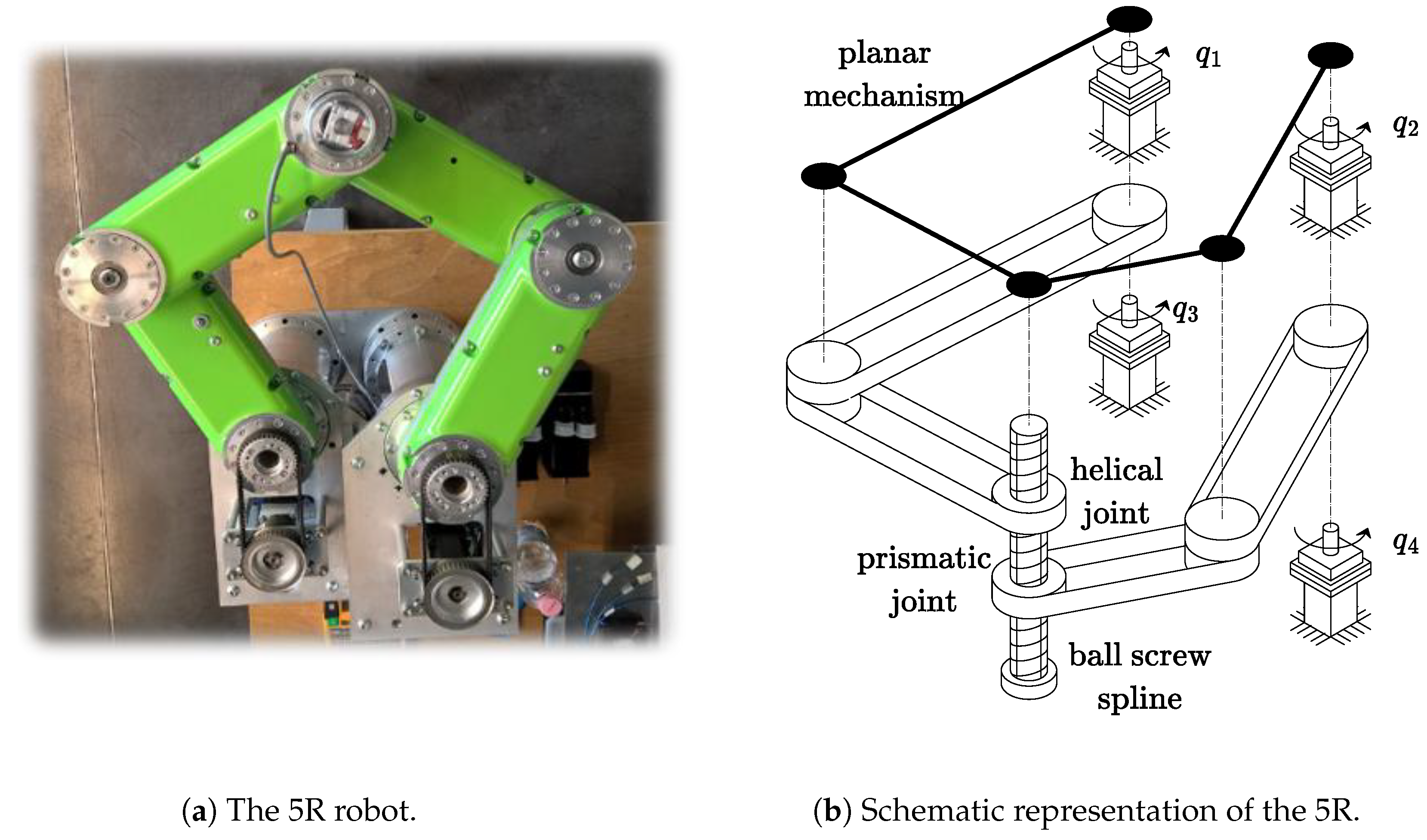
3. Case Study Description

A meaningful case study for the proposed approach is constituted by a 4-DOF 5R manipulator designed for fast pick and place applications. Similarly to more commonly used 4-DOF SCARA manipulators, the 5R uses a screw-spline mechanism for the roto-translation of the end-effector along and around the vertical axis. As depicted in Figure 6, the in-plane motion of the 5R’s end-effector is obtained thanks to a planar mechanism that features two parallel kinematic chains actuated by two electric motors fixed to the frame of the robot.

In Figure 7, the notable points and angles needed to describe the planar linkage are shown. It should be noted that the actuated angles $q_1$ and $q_2$ are constrained to rotate within bounds enforced by mechanical endstops. In particular:

$$\begin{array}{cc}\hfill q_{1,min}& =60{}^{\circ }\le q_1\le q_{1,max}={210}^{\circ }\hfill \end{array}$$

(33)

$$\begin{array}{cc}\hfill q_{2,min}& =-30{}^{\circ }\le q_2\le q_{2,max}={150}^{\circ }.\hfill \end{array}$$

(34)

Since the mechanical endstops are not symmetrical, the actual workspace will also be asymmetrical, despite the symmetry of the idealized kinematic scheme.

One peculiarity of this manipulator is constituted by the timing belt transmission systems housed inside the links, which allow to actuate the screw-spline using two additional brushless motors also attached to the robot’s fixed frame. Interestingly, this mechanical arrangement leads not only to the reduction of the moving mass but also to the complete kinematic and dynamic decoupling between the motions of the screw-spline and of the planar arms.

This is due to the unitary transmission ratio of the belt transmission systems and to the negligible friction torques of the ball bearings used to constrain the pulleys and the links. Under these conditions, it can be shown that the motion of the planar linkage and of the ball-screw-spline do not display a mutual influence; the former is exclusively determined by generalized coordinates $q_1$ and $q_2$ and motor torques ${\tau }_1$ and ${\tau }_2$, whereas the latter depends only on coordinates $q_3$ and $q_4$ and motor torques ${\tau }_3$ and ${\tau }_4$. Without introducing further assumptions, then, these two sub-systems can be analysed separately. In particular, the kinematics and dynamics of the screw-spline mechanism are invariant with respect to the joint configuration and are thus fully described by a constant Jacobian matrix. Let $z_{ee}$ and ${\varphi }_{ee}$ be the vertical position and the rotation of the end effector; let $q_3$ and $q_4$ be the joint coordinates associated, respectively, to the helical and to the prismatic joints constraining the screw-spline. The following kinematic relationships hold:

$$\begin{array}{c}\hfill \left[\begin{array}{c}{z}_{ee}\\ {\varphi }_{ee}\end{array}\right]={\displaystyle \frac{1}{2\pi }}\left[\begin{array}{cc}-p_{ss}& p_{ss}\\ 0& 2\pi \end{array}\right]=\left[\begin{array}{c}{q}_3\\ q_4\end{array}\right].\end{array}$$

(35)

The kinetic and potential energies of the screw-spline can therefore be expressed with respect to the joint variables as follows:

$$\begin{array}{ccc}\hfill T_{ss}& =& {\displaystyle \frac{1}{2}}\left((J_3+{\displaystyle \frac{m_{ee}{p}_{ss}^2}{4{\pi }^2}}){\dot{q_{}}}_3^2+(J_4+{\displaystyle \frac{m_{ee}{p}_{ss}^2}{4{\pi }^2}}+J_{ee}){\dot{q_{}}}_4^2-{\displaystyle \frac{m_{ee}{p}_{ss}^2}{2{\pi }^2}}{\dot{q_{}}}_3{\dot{q_{}}}_4\right)\hfill \end{array}$$

(36)

$$\begin{array}{ccc}\hfill U_{ss}& =& m_{ee}g{\displaystyle \frac{p_{ss}}{2\pi }}(q_4-q_3).\hfill \end{array}$$

(37)

The kinematics of the planar mechanism were instead obtained from the in-plane closure equation:

$$\begin{array}{c}\hfill \overrightarrow{O{S}_1}+\overrightarrow{S_1{E}_1}+\overrightarrow{E_{1}P}=\overrightarrow{O{S}_2}+\overrightarrow{S_2{E}_2}+\overrightarrow{E_{2}P}.\end{array}$$

(38)

The Jacobian matrices relating the velocities ${\dot{E}}_1$ and ${\dot{E}}_2$ to the joint velocities ${\dot{q_{}}}_1$ and ${\dot{q_{}}}_2$ can be trivially written as:

$$\begin{array}{ccc}\hfill {\mathit{D}}_{E,1}& =& l_{prox}\left[\begin{array}{cc}-sin\left(q_1\right)& 0\\ cos\left(q_1\right)& 0\end{array}\right]\hfill \end{array}$$

(39)

$$\begin{array}{ccc}\hfill {\mathit{D}}_{E,2}& =& l_{prox}\left[\begin{array}{cc}0& -sin\left(q_2\right)\\ 0& cos\left(q_2\right)\end{array}\right].\hfill \end{array}$$

(40)

The Jacobian analysis of the 5R end-effector kinematics is performed in such a way as to assign a clear geometric interpretation to the semi-Jacobian matrices, which relate the velocity at the joints to the velocity at the end-effector. These are:

$$\begin{array}{c}\hfill \left[\begin{array}{c}{(P-E_1)}^{\top }\\ {(P-E_2)}^{\top }\end{array}\right]\dot{P}=\left[\begin{array}{c}{(P-E_1)}^{\top }{\mathit{D}}_{E,1}\\ {(P-E_2)}^{\top }{\mathit{D}}_{E,2}\end{array}\right]\left[\begin{array}{c}{\dot{q_{}}}_1\\ {\dot{q_{}}}_2\end{array}\right].\end{array}$$

(41)

From the analysis of these two matrices, it emerges that the singular configurations for the 5R are those for which two consecutive links are collinear. As will be shown, this characterization makes it straightforward to geometrically detect configurations that are approaching a singularity and to isolate a singularity-free portion of the workspace. A more in-depth discussion of the singularities for the five bar linkage can be found in [33].

Multiplying both sides of Equation (41) by the inverse of the matrix appearing on the left-hand-side, it is possible to highlight the Jacobian matrix relating the joint velocities ${q_{}}_1$ and ${q_{}}_2$ to the planar velocity at the end-effector:

$$\begin{array}{c}\hfill \dot{P}={\mathit{D}}_P\left[\begin{array}{c}{\dot{q_{}}}_1\\ {\dot{q_{}}}_2\end{array}\right].\end{array}$$

(42)

The distal angles ${\phi }_{dist,1}$ and ${\phi }_{dist,2}$ can be expressed as:

$$\begin{array}{c}\hfill {\phi }_{dist,j}=arctan\left({\displaystyle \frac{y_P-y_{E_j}}{x_P-x_{E_j}}}\right).\end{array}$$

(43)

Since the Jacobian matrices ${\mathit{D}}_P$, ${\mathit{D}}_{E,1}$, and ${\mathit{D}}_{E,2}$ have already been made explicit, it is straightforward to find the Jacobian matrices ${\mathit{D}}_{\phi ,dist,j}$ relating ${\dot{\phi }}_{dist,j}$ to the joint velocities ${\dot{q_{}}}_1$ and ${\dot{q_{}}}_2$. Similarly, the Jacobian matrices of the centers of mass $G_{p1}$, $G_{p2}$, $G_{d1}$, $G_{d2}$ of each link can be easily deduced from ${\mathit{D}}_{E,1}$, ${\mathit{D}}_{E,2}$, ${\mathit{D}}_{\phi ,dist,1}$, ${\mathit{D}}_{\phi ,dist,2}$, and ${\mathit{D}}_P$.

Assuming that the planar mechanism operates in the horizontal plane, the potential energy $U_{5R}$ of the 5R is constant; the kinetic energy of the planar system, on the other hand, can be written as:

$$\begin{array}{cc}\hfill T_{5R}={\displaystyle \frac{1}{2}}\left[\begin{array}{cc}{\dot{q_{}}}_1& {\dot{q_{}}}_2\end{array}\right](& m_{prox,1}{\mathit{D}}_{G,p1}^{\top }{\mathit{D}}_{G,p1}+\hfill \\ \hfill & m_{prox,2}{\mathit{D}}_{G,p2}^{\top }{\mathit{D}}_{G,p2}+\hfill \\ \hfill & m_{dist,1}{\mathit{D}}_{G,d1}^{\top }{\mathit{D}}_{G,d1}+\hfill \\ \hfill & m_{dist,2}{\mathit{D}}_{G,d2}^{\top }{\mathit{D}}_{G,d2}+\hfill \\ \hfill & J_{dist,1}{\mathit{D}}_{\phi ,dist,1}^{\top }{\mathit{D}}_{\phi ,dist,1}+\hfill \\ \hfill & J_{dist,2}{\mathit{D}}_{\phi ,dist,2}^{\top }{\mathit{D}}_{\phi ,dist,2}+{\mathit{J}}_{prox})\left[\begin{array}{c}{\dot{q_{}}}_1\\ {\dot{q_{}}}_2\end{array}\right],\hfill \end{array}$$

(44)

with:

$${\mathit{J}}_{prox}=\left[\begin{array}{cc}{J}_{prox,1}& 0\\ 0& J_{prox,2}\end{array}\right].$$

(45)

The Lagrangian function of the entire system is:

$$\begin{array}{c}\hfill \mathcal{L}(\mathit{q},\dot{\mathit{q}})=T_{5R}+T_{ss}-U_{5R}-U_{ss}.\end{array}$$

(46)

Consequently, the dynamics of the system were obtained using Lagrange equations:

$$\begin{array}{c}\hfill {\displaystyle \frac{{\mathrm{d}}^{}}{\mathrm{d}{t}^{}}}{\displaystyle \frac{{\partial }^{}\mathcal{L}}{\partial {{\dot{q_{}}}_k}^{}}}-{\displaystyle \frac{{\partial }^{}\mathcal{L}}{\partial {{q_{}}_k}^{}}}={\tau }_k\end{array}$$

(47)

and afterwards were rearranged to obtain relationships formally identical to Equation (11). A more detailed discussion of the dynamics of the 5R robot can be found in [34].

The selection of the transmission and of the power drive systems was performed according to the procedure detailed in [32]. All the parameters related to the actuation and transmission systems are thus fully defined and reported in

Table 1. Main parameters of the four servoaxes.

	Servoaxis 1	Servoaxis 2	Servoaxis 3	Servoaxis 4
${\tau }_{pds,rated},\left[\mathrm{N} \mathrm{m}\right]$	0.7	0.7	0.36	0.36
${\tau }_{pds,max},\left[\mathrm{N} \mathrm{m}\right]$	1.4	1.4	0.72	0.72
${\omega }_{pds,max},\left[\mathrm{rad} {\mathrm{s}}^{-1}\right]$	500	500	500	500
$J_m,\left[\mathrm{k}\mathrm{g} {\mathrm{m}}^2\right]$	$1.7\times {10}^{-5}$	$1.7\times {10}^{-5}$	$2.4\times {10}^{-6}$	$2.4\times {10}^{-6}$
${\eta }_t$	$\sim 1$	$\sim 1$	$\sim 1$	$\sim 1$
$J_t,\left[\mathrm{k}\mathrm{g} {\mathrm{m}}^2\right]$	$2.485\times {10}^{-5}$	$2.485\times {10}^{-5}$	$2.05\times {10}^{-5}$	$2.05\times {10}^{-5}$
$i_t$	64	64	10	10

. Accordingly, the contributions associated with the motors and with the transmissions are included as appropriate within the overall dynamics of the system.

During the motion, the manipulator should not cross any singular configuration, change its assembly, or violate the physical constraints introduced by the mechanical endstops. The actual workspace is consequently reduced to the configurations that satisfy the following conditions:

$$\begin{array}{ccc}\hfill q_1& \ge & q_{1,min}\hfill \end{array}$$

(48)

$$\begin{array}{ccc}\hfill q_1& \le & q_{1,max}\hfill \end{array}$$

(49)

$$\begin{array}{ccc}\hfill q_2& \ge & q_{2,min}\hfill \end{array}$$

(50)

$$\begin{array}{ccc}\hfill q_2& \le & q_{2,max}\hfill \end{array}$$

(51)

$$\begin{array}{ccc}\hfill \overrightarrow{E_{1}P}·\mathit{j}\left(\overrightarrow{S_1{E}_1}\right)& \le & 0\hfill \end{array}$$

(52)

$$\begin{array}{ccc}\hfill \overrightarrow{E_{2}P}·\mathit{j}\left(\overrightarrow{S_2{E}_2}\right)& \ge & 0\hfill \end{array}$$

(53)

$$\begin{array}{ccc}\hfill \overrightarrow{E_{avg}P}·\mathit{j}\left(\overrightarrow{E_1{E}_2}\right)& \ge & 0,\hfill \end{array}$$

(54)

with

$$\begin{array}{ccc}\hfill E_{avg}& =& {\displaystyle \frac{1}{2}}(E_1+E_2)\hfill \end{array}$$

(55)

$$\begin{array}{ccc}\hfill \mathit{i}(\overrightarrow{AB})& =& \overrightarrow{AB}/\Vert \overrightarrow{AB}\Vert \hfill \end{array}$$

(56)

$$\begin{array}{ccc}\hfill \mathit{j}(\overrightarrow{AB})& =& {\left[\begin{array}{cc}-i_2(\overrightarrow{AB}),& i_1(\overrightarrow{AB})\end{array}\right]}^{\top }.\hfill \end{array}$$

(57)

In particular, the enforcement of inequalities (48)–(51) and conditions (52)–(54) (which were determined from the analysis of Equation (41)) prevents the crossing of singular configurations and the change of assembly or operating mode. In Figure 8, the useful workspace resulting from inequalities (48)–(54) is shown, both in the taskspace and in the jointspace. The boundaries of the filled area either are determined by the mechanical endstops or correspond to singularities. Inside the admissible area, the reciprocal condition number:

$$\begin{array}{c}\hfill r_{\sigma }=\sqrt{{\displaystyle \frac{{\sigma }_{min}}{{\sigma }_{max}}}},\end{array}$$

(58)

with ${\sigma }_{min}$ and ${\sigma }_{max}$ being the minimum and maximum singular values of the matrix ${\mathit{D}}_P{\mathit{D}}_P^{\top }$, is represented. A further condition fixing a minimum value for the reciprocal condition number can be defined in order to stay sufficiently clear of singular configurations:

$$\begin{array}{c}\hfill r_{\sigma }\ge {\delta }_{\sigma }.\end{array}$$

(59)

For the first numerical example detailed below, the parameter ${\delta }_{\sigma }$ has been set to $0.1$; for the second application, instead, we selected ${\delta }_{\sigma }=0.2$.

The main properties of the robot are:

• length of the proximal links $l_{prox}=250$ mm;
• length of the distal links $l_{dist}=250$ mm;
• frame length $l_f=180$ mm;
• mass of the proximal links $m_{prox,1}=m_{prox,2}=2.9$ kg;
• mass of the distal links $m_{dist,1}=m_{dist,2}=2.9$ kg;
• barycentric inertia of the proximal links $J_{prox,1}=J_{prox,2}$ = 5.22 × 10⁻² kg m²;
• barycentric inertia of the distal links $J_{dist,1}=J_{dist,2}$ = 5.22 × 10⁻² kg m²;
• mass of the screw-spline and of the end-effector $m_{ee}=0.36$ kg;
• screw-spline pitch $p_{ss}=2$ mm;
• rotational inertia of the end-effector $J_{ee}$ = 6.40 × 10⁻⁶ kg m²;
• rotational inertia of the transmission system actuating the screw-spline helical joint $J_3$ = 1.20 × 10⁻⁶ kg m²;
• rotational inertia of the transmission system actuating the screw-spline prismatic joint $J_4$ = 1.20 × 10⁻⁶ kg m².

The mass parameters of the links also take into account the masses of the pulleys and belts.

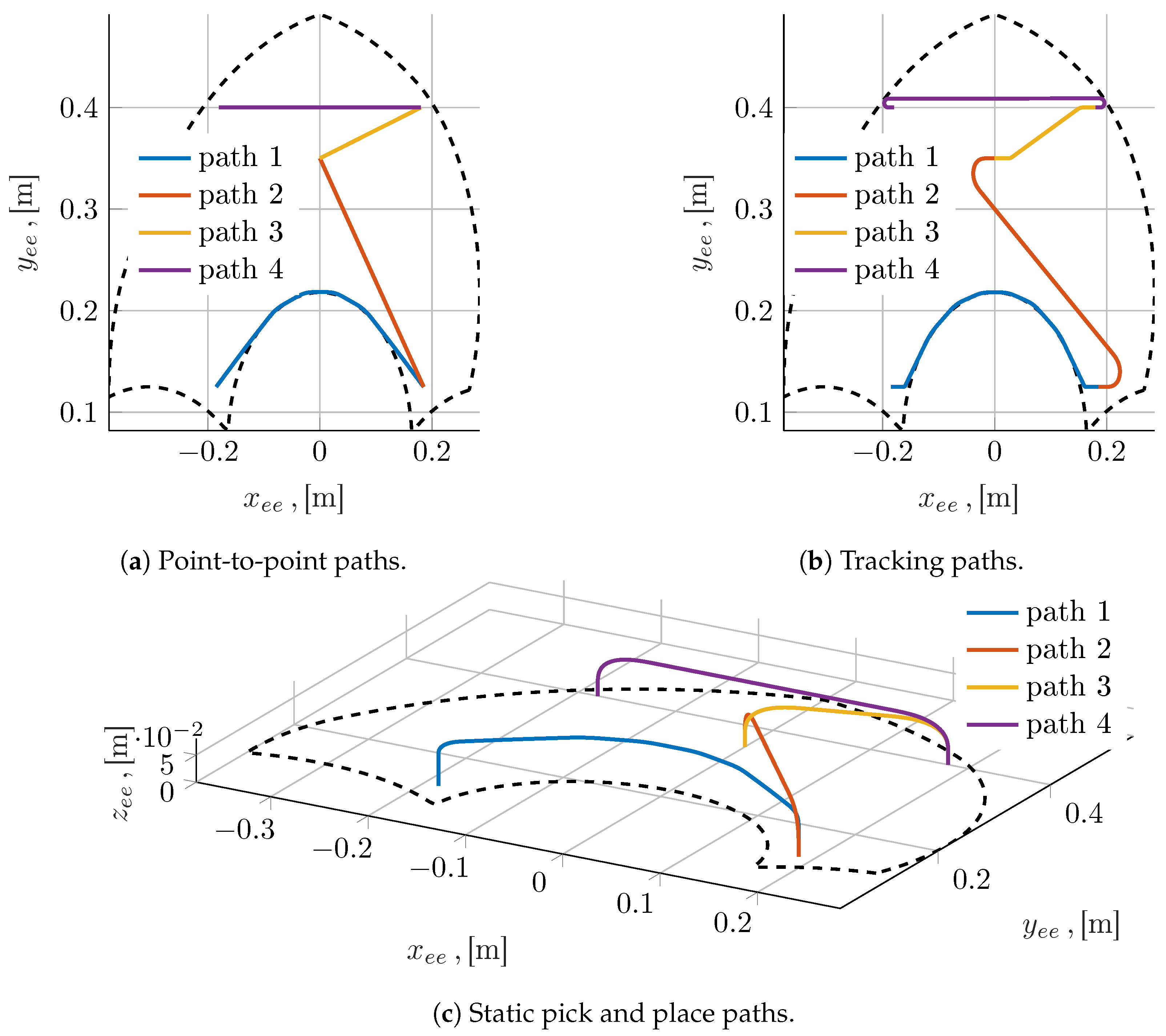
Geometric Planning for the 5R Robot

The GTP here proposed is configured for the parametrization of two different types of motions:

• stationary pick and place tasks, where the initial and final velocities are null;
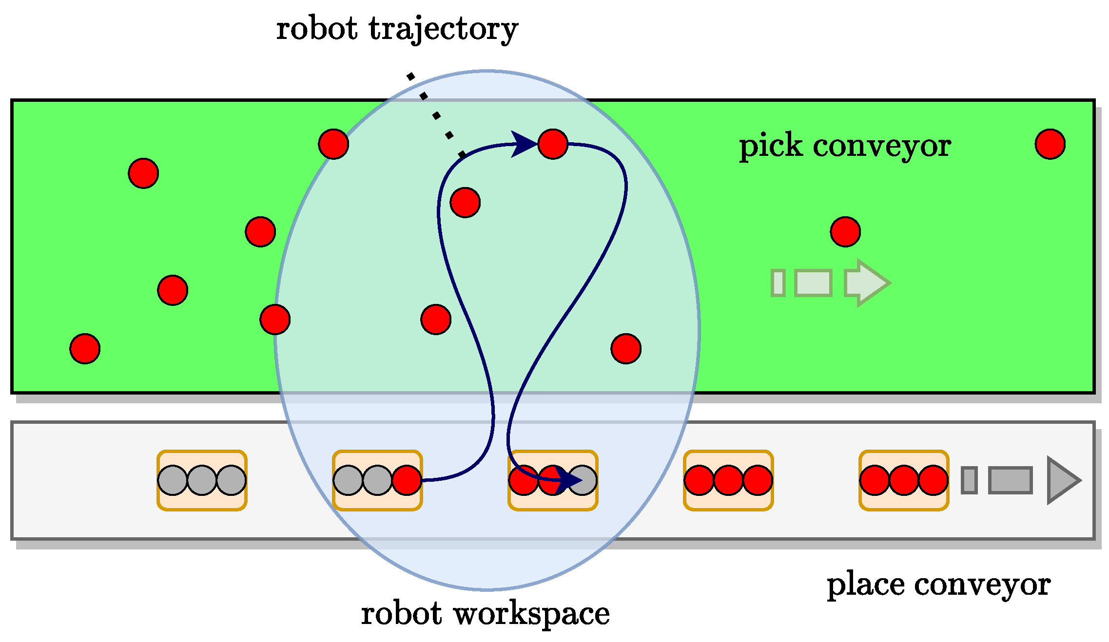
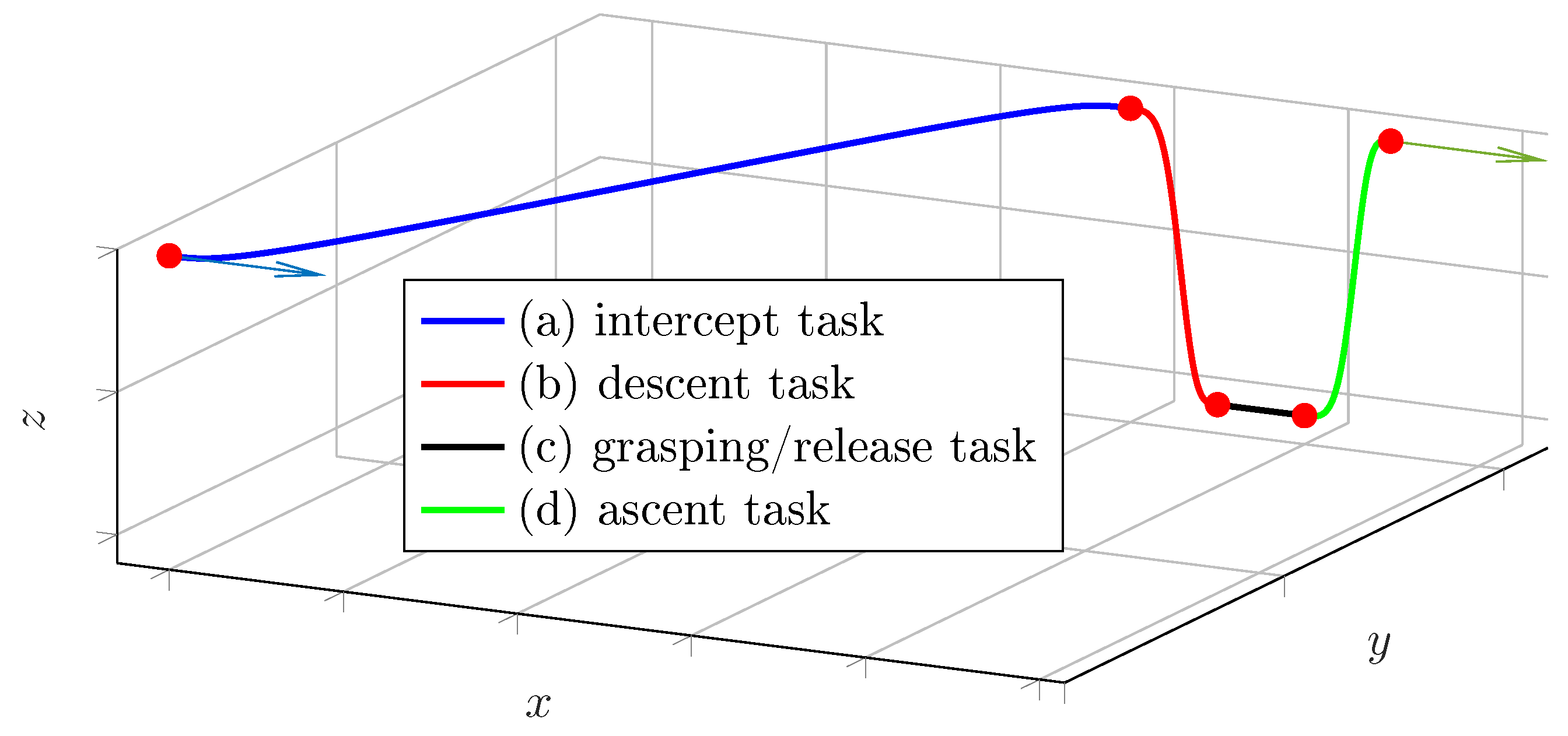
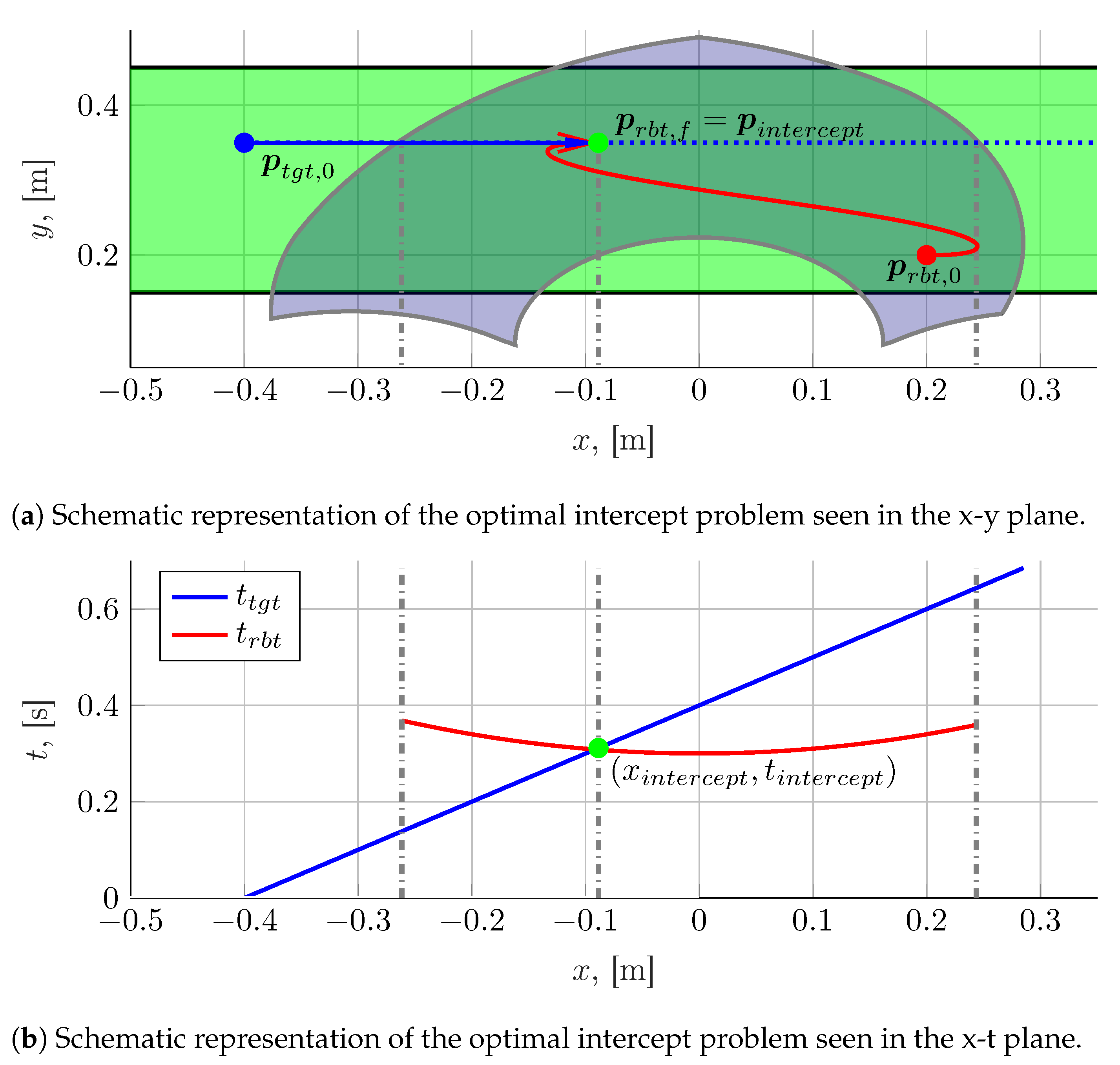
• on-the-fly pick and place tasks, such as those represented in Figure 1, where the initial and final velocities are non-null and aligned to the x-axis.

For stationary pick and place motions, a simple portal-like trajectory is sufficient. On the contrary, for on-the-fly manipulation tasks, more complex composite trajectories, such as the one represented qualitatively in Figure 9, are needed.

In that figure, it can be seen that the on-the-fly manipulation trajectory is constituted by four portions:

• an intercept motion (a), which happens in a slightly elevated plane and which terminates with an x-y position, a rotation and a velocity that match those of the pick and place target; its terminal position can be found, as will be shown, by solving the optimal intercept problem;
• a descent motion (b) through which the gripper approaches the target from above;
• a grasping/release motion (c) during which the gripping device operates to grasp or release the item;
• an ascent motion (d) through which the gripper attains the proper vertical clearance.

The motions (b) (c) and (d) constitute the tracking phase proper, since all have a velocity along the x-axis that matches the one of the pick and place target. The duration of motion (c) is determined by the operating time of the gripping device and therefore is not a target for optimization. The motions (b) and (d) are usually quite short, as the vertical excursion is typically very limited in pick and place applications. For the 5R robot considered in the example, moreover, the optimal time needed to perform a given vertical motion is a function only of the vertical displacement itself, due to the screw-spline being a linear time-invariant system decoupled from the planar five bar mechanism. Once the vertical displacement is fixed, the task times of (b) and (d) are known constants. In particular, considering a vertical displacement of the end-effector $\Delta z_{ee}=$ 20 mm, we obtained the following task times:

$$\begin{array}{ccc}\hfill T_{task\left(b\right)}& =& 0.07682 \mathrm{s}\hfill \end{array}$$

(60)

$$\begin{array}{ccc}\hfill T_{task\left(d\right)}& =& 0.07682 \mathrm{s}.\hfill \end{array}$$

(61)

The fact that the $T_{task\left(b\right)}$ is equal to $T_{task\left(d\right)}$ is not surprising, given the symmetry of the problem, in which gravity:

• assists the acceleration phase of the descent motion (b);
• opposes the deceleration phase of the descent motion (b);
• opposes the acceleration phase of the ascent motion (d);
• assists the deceleration phase of the ascent motion (d).

In cases featuring different robots, it is entirely possible to construct time maps for motions (b) and (d) using the general approach here proposed. It should be remarked that, in general, the execution times of tasks (b) and (d) are a function only of the starting position and velocity; the dimensionality of the problem is therefore lower compared to the one associated with motion (a). Finally, it can be noted that the map associated with motion (a) needs to be evaluated more frequently for the solution of the optimal intercept problem, whereas maps for motions (b) and (d) are not invoked for this purpose. It can be easily observed in Figure 8 that the useful workspace is not convex, neither in the task space nor in the joint space. The geometric planning, even for simple point-to-point trajectories, is therefore not entirely straightforward. A variety of solutions might be adopted; the one here proposed features minimum-length trajectories planned in the task space.

This choice is motivated by the fact that, already, for ${\delta }_{\sigma }=0.1$, the useful workspace is a normal domain, clearly having two function-like lower and upper boundaries, which are denoted in the following as $y_{lb}\left(x_{ee}\right)$, $y_{ub}\left(x_{ee}\right)$ and which can be numerically evaluated, e.g., using a zero-finding algorithm on the boolean function obtained from the simultaneous enforcement of Inequalities (48)–(54) and (59). This, in turn, allowed us to set up the geometric planning of a point-to-point minimum length motion as a convex quadratic program (CQP) that yields a control polyline, which can be easily postprocessed in order to fully define the trajectory.

Consider at first only the planar motion. Fixing the feasible initial and final positions ${\mathit{p}}_{\mathit{s}}$ and ${\mathit{p}}_{\mathit{f}}$ of the manipulator, the coordinates $x_{ee,s}$, $y_{ee,s}$, $x_{ee,f}$, and $y_{ee,f}$ are fixed. Let ${\mathit{x}}_{sol}$ and ${\mathit{x}}_{constr}$ be equally spaced arrays of $n_{cqp}$ and $m_{cqp}$ elements each:

$$\begin{array}{ccc}\hfill {\mathit{x}}_{sol}& =& \left[\begin{array}{cccc}{x}_{sol,1}=x_{ee,s},& x_{sol,2},& \dots ,& x_{sol,n_{cqp}}=x_{ee,f}\end{array}\right]\hfill \end{array}$$

(62)

$$\begin{array}{ccc}\hfill {\mathit{x}}_{constr}& =& \left[\begin{array}{cccc}{x}_{constr,1}=x_{ee,s},& x_{constr,2},& \dots ,& x_{constr,m_{cqp}}=x_{ee,f}\end{array}\right].\hfill \end{array}$$

(63)

Let $\mathit{y}=\left[\begin{array}{cccc}{y}_{ee,1},& y_{ee,2},& \dots ,& y_{ee,n_{cqp}}\end{array}\right]$ be $n_{cqp}$ decision variables.

Finally, let ${\mathit{N}}_{{\mathit{x}}_{sol}}\left(x_{ee}\right)$ be the shape functions yielding the linear interpolation of $\mathit{y}$ over ${\mathit{x}}_{sol}$. The constraints of the problem can then be written in linear form as:

$$\begin{array}{ccc}\hfill y_{ee,1}& =& y_{ee,s}\hfill \end{array}$$

(64)

$$\begin{array}{ccc}\hfill y_{ee,n_{cqp}}& =& y_{ee,f}\hfill \end{array}$$

(65)

$$\begin{array}{ccc}\hfill {\mathit{N}}_{{\mathit{x}}_{sol}}^{\top }\left(x_{constr,k}\right)\mathit{y}& \le & y_{ub}\left(x_{constr,k}\right)\hfill \end{array}$$

(66)

$$\begin{array}{ccc}\hfill {\mathit{N}}_{{\mathit{x}}_{sol}}^{\top }\left(x_{constr,k}\right)\mathit{y}& \ge & y_{lb}\left(x_{constr,k}\right)\hfill \end{array}$$

(67)

for $k=1,\dots ,m_{cqp}$. Finally, as the quadratic cost function (which has the same minimum point of the squared-length function):

$$\begin{array}{c}\hfill L^2=\sum _{i=2}^{n_{cqp}}{(y_{ee,i}-y_{ee,i-1})}^2\end{array}$$

(68)

admits a positive definite Hessian matrix, the minimum length polyline joining the initial and final configurations can be found as the result of a convex quadratic program.

The minimum length polyline so obtained constitutes the basic solution from which a variety of motions can be easily constructed, as exemplified in Figure 10. For example, it is entirely straightforward to add to each point a desired out-of-plane displacement, e.g., to obtain a motion suitable for stationary pick and place actions; the rotational coordinate of the end effector can also be added as dictated by the requisites for the specific application. It is then possible to join two consecutive line segments with circular arcs in order to obtain a $C^1$ continuous path whose arc parameter is easily computed. Furthermore, a smoothing operation can be applied to yield a $C^2$ path; given the fact that the geometric primitives we used are integrable in closed form, the filter we developed is constituted by an analytical integral average over a window, which slides along the arc parameter of the curve and whose size is calculated in relation to the length of each constitutive segment or arc. An analogous idea can be found in [28], in which, however, a discrete time FIR filter is used to obtain continuous geometric accelerations.

In addition, the changes of directions needed for on-the-fly pick and place operations can be prepended or appended to the trajectory as required to obtain the proper alignment with the tracking direction. These trajectories, in particular, are constructed assuming that the items are moving along one or more conveyor belts aligned to the $x_{ee}$-axis and such that the end-effector moves in plane in order to reach the position above the target with the velocity needed to initiate the subsequent descent, grasping/release, and ascent motions.

Since both stationary and on-the-fly pick and place tasks have been considered at the geometric level, two families of parametric tasks are to be optimized in terms of execution times. Of these families, the former is characterized by null initial velocities, while the velocity boundary conditions of the latter are free parameters appearing alongside the initial and final positions. The task time models for these two kinds of motions accept therefore a different number of input parameters, and, as detailed in the following discussion, they are characterized by different internal architectures. Despite these differences, they offer a very similar query interface and are trained and deployed in an almost identical manner, showcasing the adaptability of the proposed method to different task typologies.

4. Computational Results and Discussion

4.1. Software and Hardware Setup

The task time datasets were generated using an in-house object-oriented C++ codebase. The main modules of our software implement:

• an abstract class representing a generic n-DOF manipulator, from which specific implementations (among which the one relative to the 5R robot) are derived;
• an abstract class representing a generic TTO, from which specific implementations are derived according to the different optimization methods;
• an abstract class representing a generic n-DOF geometric path, with its derived implementations;
• a set of routines implementing the GTP for the 5R robot;
• a utility class dedicated to the multithreaded generation of the dataset.

To solve the linear program (32), we use the Gnu Linear Programming Kit (GLPK); we treat the quadratic optimization problem arising during the geometric trajectory planning using the OSQP solver [35]. To accurately compute the task time $T_{task}$ according to Equation (23), we implemented the algorithm proposed by [36]. This method was selected due to its ability to treat integrable singularities at finite points, which, in our case, occur when the motion has null velocities at the extremities; in those cases, we allowed small initial and final accelerations to mathematically ensure integrability.

Each model was trained on a dataset of ${10}^6$ trajectories, whose initial and final poses were sampled according to a uniform random distribution in the task space, considering:

• a rotation range for the end-effector equal to $\Delta {\varphi }_{ee\in }\left[-\pi ,\pi \right]$;
• a range for the initial and final velocities equal to $v\in$ [0.05 m s⁻¹, 0.5 m s⁻¹];
• initial and final x-y positions that satisfy inequalities (48)–(54) and (59).

The neural network architectures were defined and trained using the PyTorch library. The main hyperparameters characterizing the training process are:

• loss function: MSE (Mean Squared Error)
• training algorithm: SGD (Stochastic Gradient Descent)
• batch size: 2048 data points.

The determination of the hyperparameters has not been automated; instead, they have been experimentally tuned in order to obtain a compromise between training speed and accuracy.

For both models, the accuracy and precision of the prediction are evaluated through the distributions of the prediction error and of the relative prediction error. The prediction error is defined as:

$$\begin{array}{ccc}\hfill {\epsilon }_{T_{task}}& =& T_{task}-{\widehat{T}}_{task},\hfill \end{array}$$

(69)

where ${\widehat{T}}_{task}$ is the task time estimate obtained from the trained model. On the other hand, the relative prediction error is defined as:

$$\begin{array}{ccc}\hfill {\epsilon }_{T_{task},\%}& =& 100{\displaystyle \frac{T_{task}-{\widehat{T}}_{task}}{T_{task}}}.\hfill \end{array}$$

(70)

Both error distributions were computed on the test dataset.

Three additional quantities that are considered to evaluate the soundness of the proposed methods are:

• ${\overline{T}}_{plan}$, the average execution time of the entire motion planning and optimization pipeline for a single trajectory;
• ${\overline{T}}_{eval,cpu}$, the average evaluation time of the task time map on a single CPU core;
• ${\overline{T}}_{eval,gpu}$, the average evaluation time of the task time map on the GPU.

These values were obtained by performing all the required computations on a machine running a Linux operating system and having the specifications detailed below:

• CPU: Intel^® Core™(Santa Clara, CA, USA) i7-8750H processor $2.2$ $\mathrm{G}$$\mathrm{Hz}$ (9 $\mathrm{M}$ cache, up to $4.1$ $\mathrm{G}$$\mathrm{Hz}$, 6 processors);
• GPU: Nvidia^® (Santa Clara, CA, USA) GeForce^® (Santa Clara, CA, USA) GTX 1050, 4 $\mathrm{G}$, GDDR5;
• RAM: 16 $\mathrm{G}$ DDR4 SO-DIMM, 2400 $\mathrm{M}$$\mathrm{Hz}$.

Clearly, the usefulness of the task time map is predicated not only on the achievement of sufficient accuracy but also on evaluation times (either ${\overline{T}}_{eval,cpu}$ or ${\overline{T}}_{eval,gpu}$) much lower than the planning time ${\overline{T}}_{plan}$. Within the scope of this work, the average evaluation time of the models is conservatively determined through the execution of the model itself within the Python3 interpreter, whereas ${\overline{T}}_{plan}$ is determined using the C++ implementations of the GTP and TTO. These quantities are summarized for both the stationary and the on-the-fly pick and place case studies in

Table 2. Comparison of the evaluation times of the neural network models and of the GTP-TTO algorithms.

Task Type	${\overline{\mathit{T}}}_{\mathit{eval},\mathit{cpu}},\left[\mathbf{\mu s}\right]$	${\overline{\mathit{T}}}_{\mathit{eval},\mathit{gpu}},\left[\mathbf{\mu s}\right]$	${\overline{\mathit{T}}}_{\mathit{plan}},\left[\mathbf{\mu s}\right]$	${\overline{\mathit{T}}}_{\mathit{plan}}/{\overline{\mathit{T}}}_{\mathit{eval},\mathit{cpu}}$	${\overline{\mathit{T}}}_{\mathit{plan}}/{\overline{\mathit{T}}}_{\mathit{eval},\mathit{gpu}}$
Stationary Pick and Place	81	6	49,419	610.11	8236.5
On-the-fly Pick and Place	2310	73	56,985	24.7	780.6

. A histogram of the planning times for a representative sample of trajectories is reported in Figure 11.

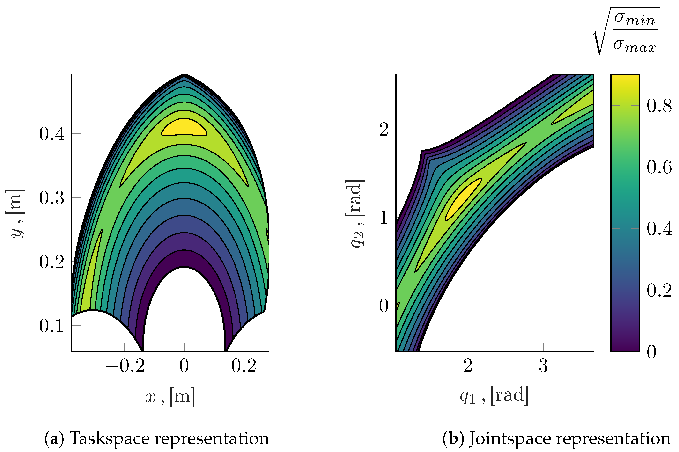
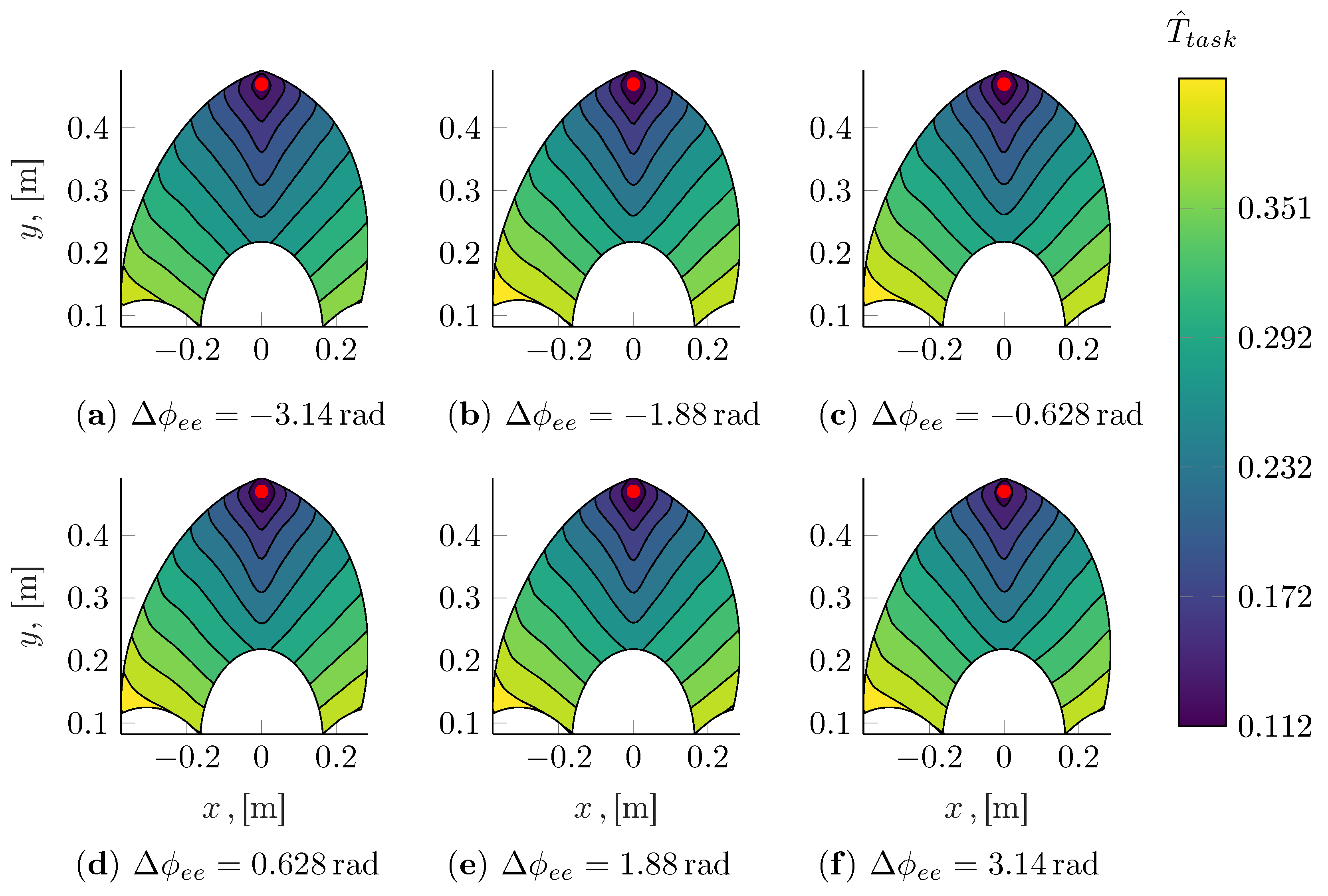
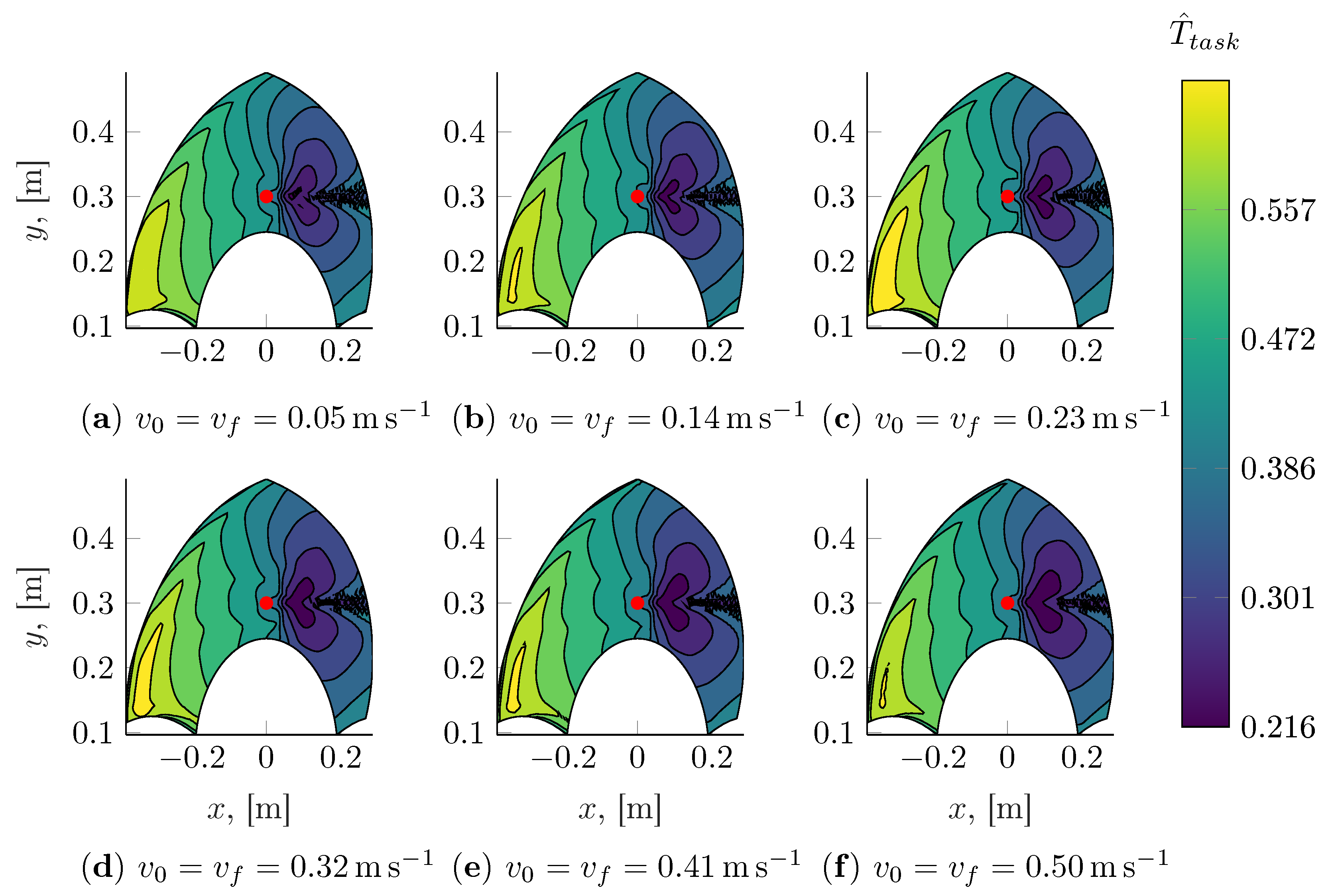
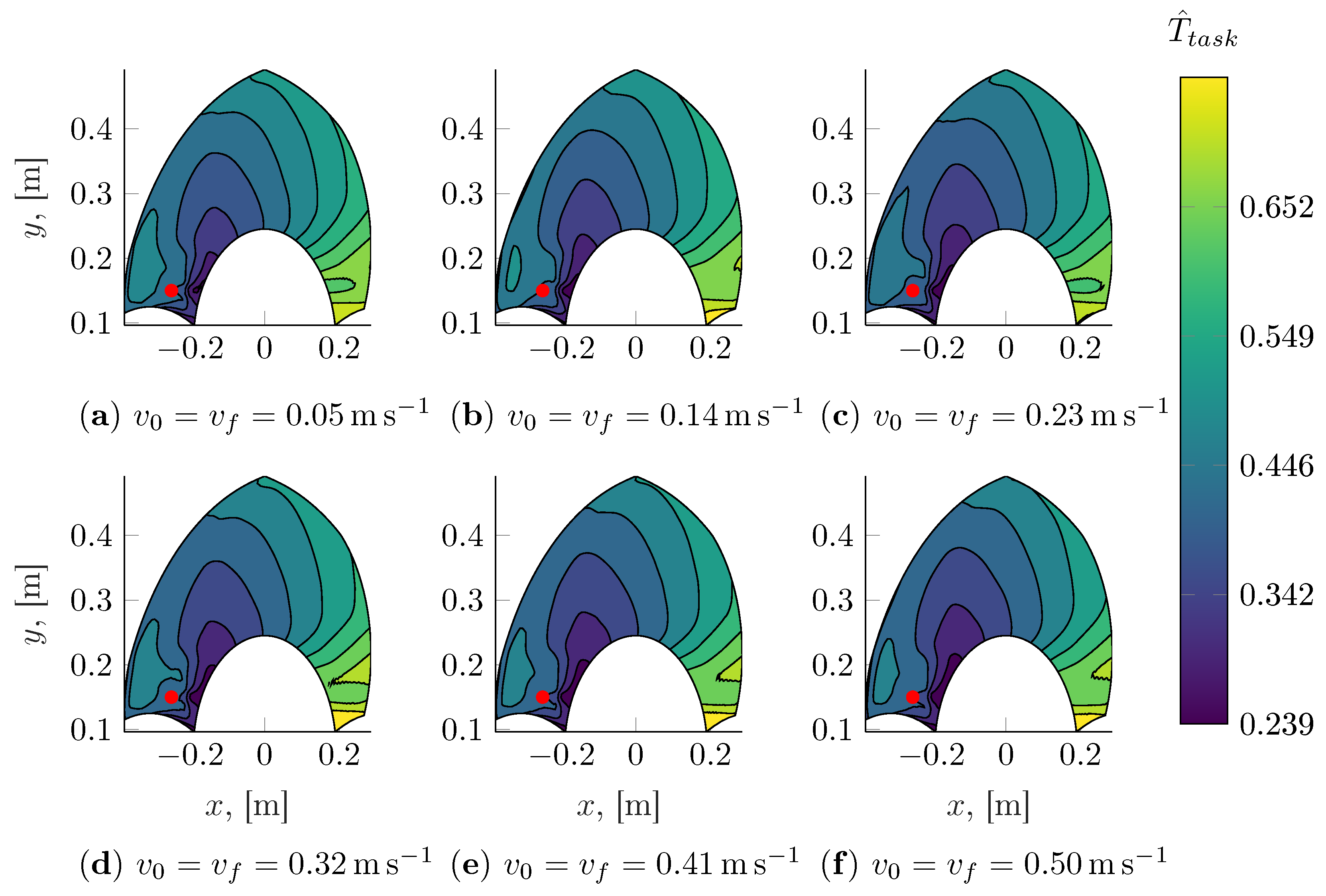
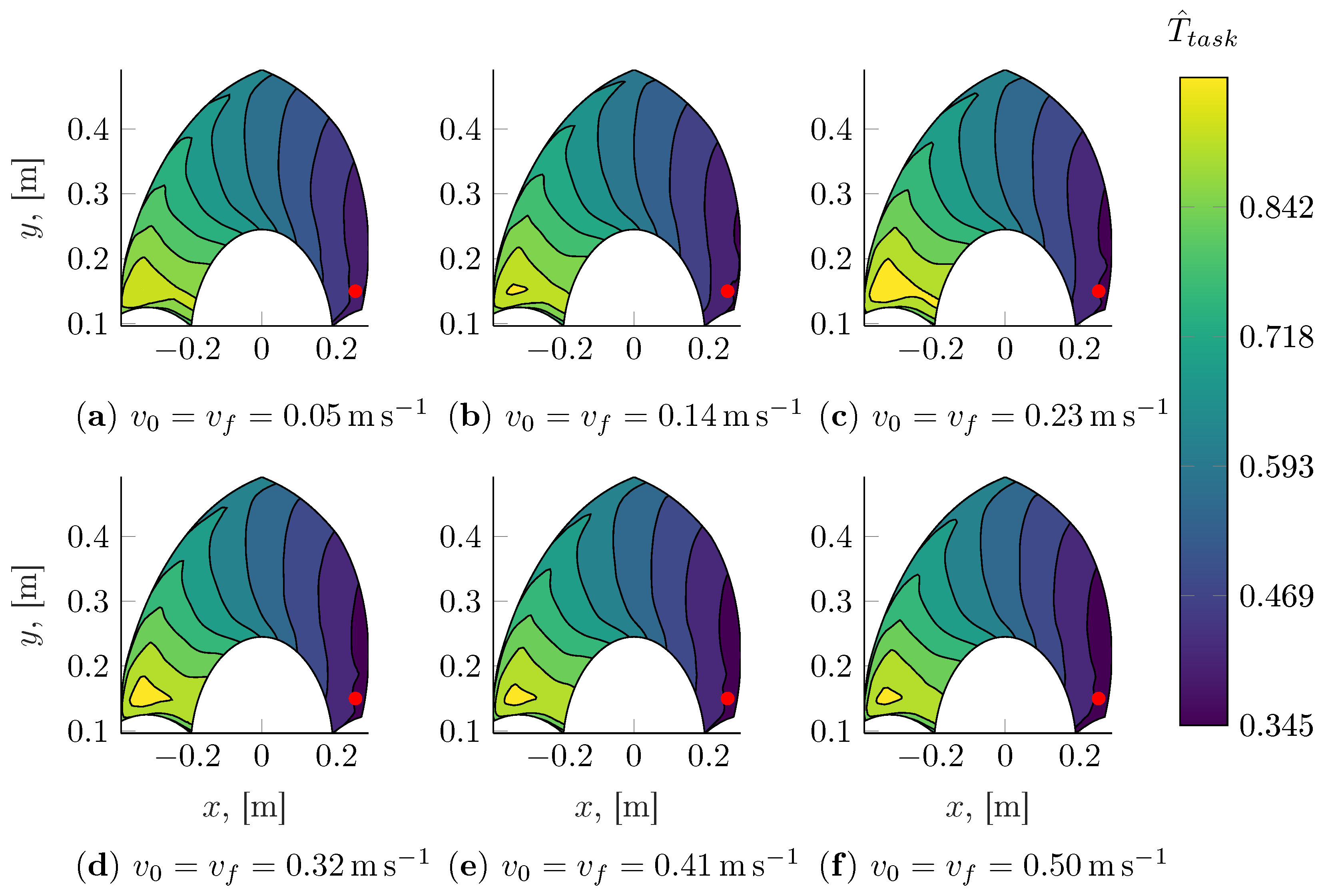
4.2. Stationary Pick and Place Task Time Map

A feedforward neural network having three hidden layers was selected; the main parameters of the network are summarized in

Table 3. Main parameters of the neural network architecture for the stationary pick and place task time map.

	Layer 1	Layer 2	Layer 3
Type	Fully connected	Fully connected	Fully connected
Activation	ReLU	ReLU	Linear
Dropout probability	0.20	0.20	0.20
$n_{in}$	5	2048	2048
$n_{out}$	2048	2048	1

.

In Figure 12, the top panel shows the histogram of the prediction error ${\epsilon }_{T_{task}}$, while the bottom one depicts the histogram of the relative prediction error ${\epsilon }_{T_{task},\%}$. These errors are small both in absolute and relative terms; therefore, the map output cannot reliably discern two tasks whose duration difference is less than the error introduced. From the time duration point of view, these tasks are practically equivalent due to the limited percentual error. Regarding the effective behavior of the robot, we can discuss two main scenarios.

In the first, the command to the robot uses the boundary conditions and the map task time ${\widehat{T}}_{task}$. Therefore, the robot executes the task in the given time. If ${\widehat{T}}_{task}>T_{task}$, the task is executed with speeds and accelerations lower than those generated by the TTO. On the contrary, if ${\widehat{T}}_{task}<T_{task}$, the task will be executed with higher speeds and accelerations, provided that the robot can reach these. In general, the TTO should optimize the task execution times considering conservative estimates of the robot’s capabilities so that the small adjustments described here remain compatible with the actual peak performances of the manipulator.

In the second, the command to the robot considers only the boundary conditions. In this case, the task execution time is $T_{task}$ due to the robot’s TTO, and the robot can realize the task. The subsequent task can be executed after the completion of the previous one.

To verify that the use of the resulting model is compatible with the time requirements of an online scheduling algorithm, we evaluated the average time needed on the one hand to evaluate the neural network and on the other to execute the GTP and the TTO processes. The average evaluation times are:

• ${\overline{T}}_{eval,cpu}=81.38 \mathrm{\mu s}$ on a single CPU core, using the Python-3 interpreter;
• ${\overline{T}}_{eval,gpu}=5.96 \mathrm{\mu s}$ on the GPU, using the Python-3 interpreter;
• ${\overline{T}}_{plan}=49.4 \mathrm{m}\mathrm{s}$ on the CPU, using the C++ implementation of the GTP and TTO.

Even without the GPU, then, it can be observed that the evaluation of the model to yield ${\widehat{T}}_{task}$ is two orders of magnitude faster than the direct evaluation of the task time $T_{task}$ using the GTP and the TTO; further and significant speedups can moreover be obtained using the GPU.

A qualitative inspection of the predicted task times ${\widehat{T}}_{task}$ was also performed as shown in Figure 13, Figure 14, Figure 15 and Figure 16. In particular, by fixing the initial pose and the total rotation of the end-effector, it is possible to visualize the task time estimate as a function of the final Cartesian coordinates of the gripper. The initial configuration is shown in the figures with a red marker. It can be seen that ${\widehat{T}}_{task}$ is positively correlated with the total displacement achieved at the end-effector. The isolines of ${\widehat{T}}_{task}$ are not, however, merely radial, as they are a more general function not only of the non-linear kinematics and dynamics of the mechanism but also of the actuation systems, whose main properties and non-linearities (namely the torque and velocity saturations) are accounted for within the overall motion planning strategy and are thus reflected in the outputs of the task time model.

In this example, the rotational displacement has a rather small effect on the total execution time of the trajectory. It can be seen, however, that for small displacements, the execution of the end-effector rotation can constitute the bottleneck of the overall motion. This fact becomes apparent only when closely focusing on the size of the region enclosed in the isoline closest to the initial configuration considered at different magnitudes of the rotational displacement.

The resulting task time map covers the entire useful workspace of the robot; during the design phase, it enables therefore greater freedom in the definition of the layout of the elements surrounding the robot; it also provides insight into the more convenient locations in which to position, e.g., the transportation systems.

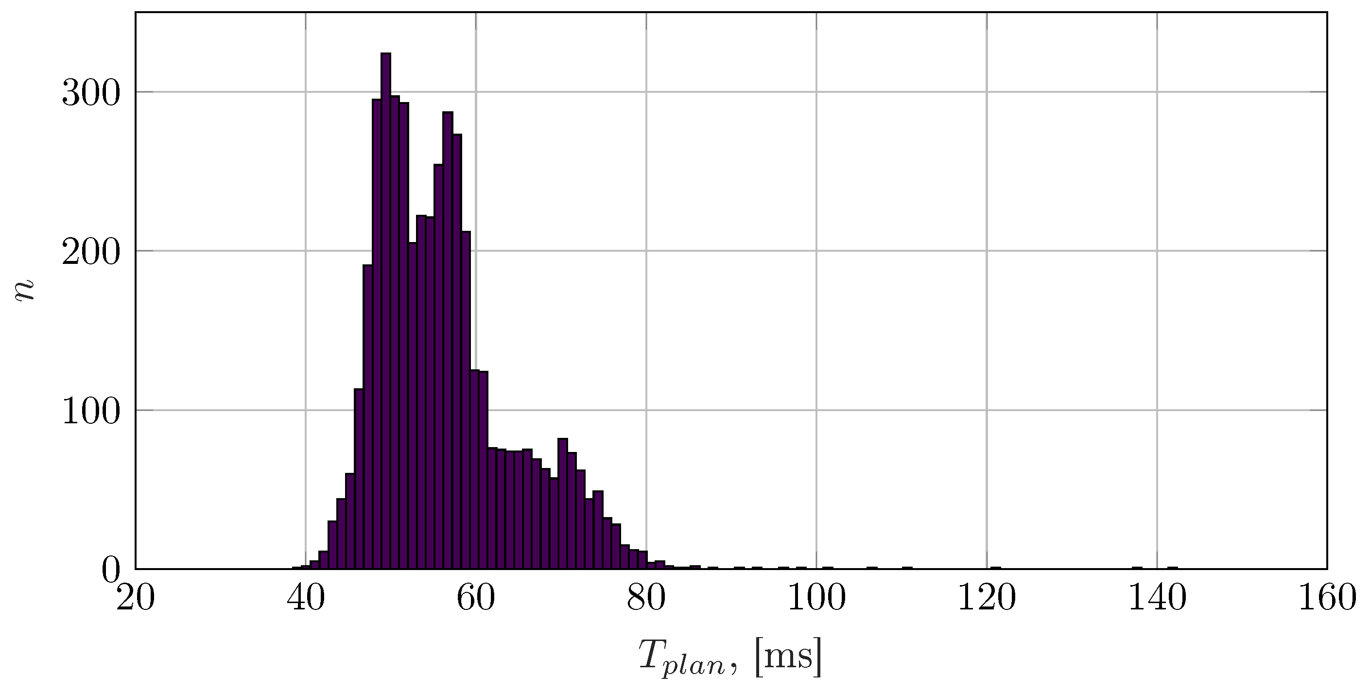
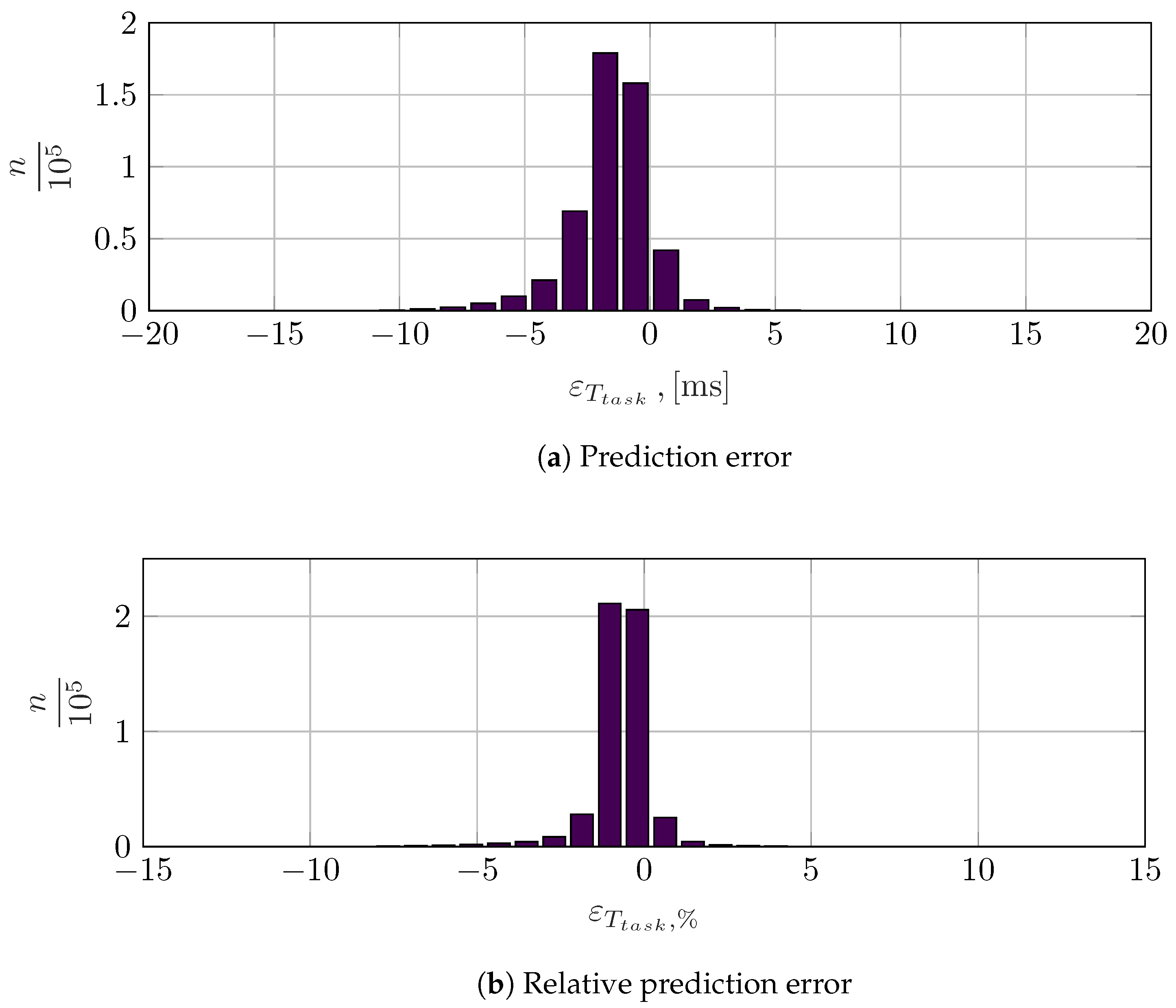
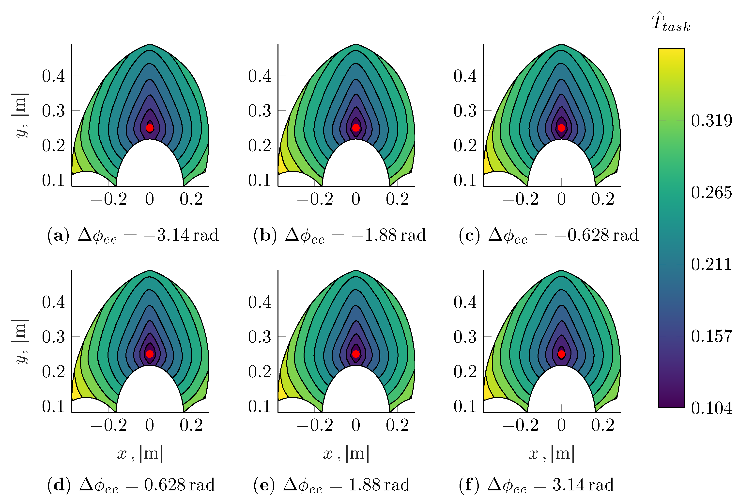
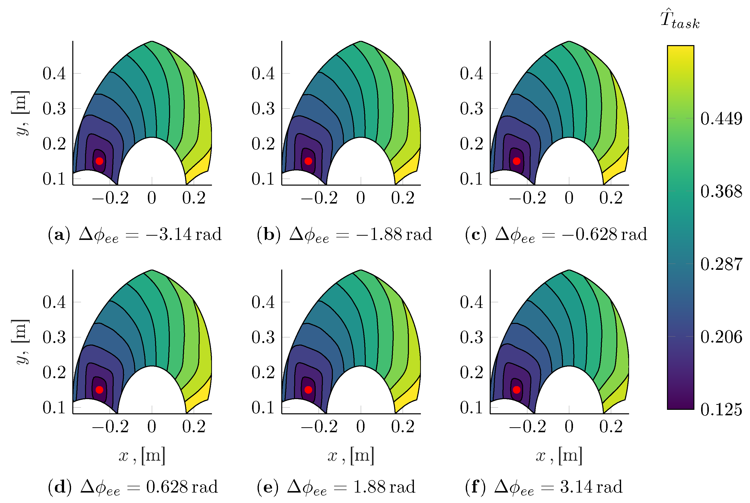
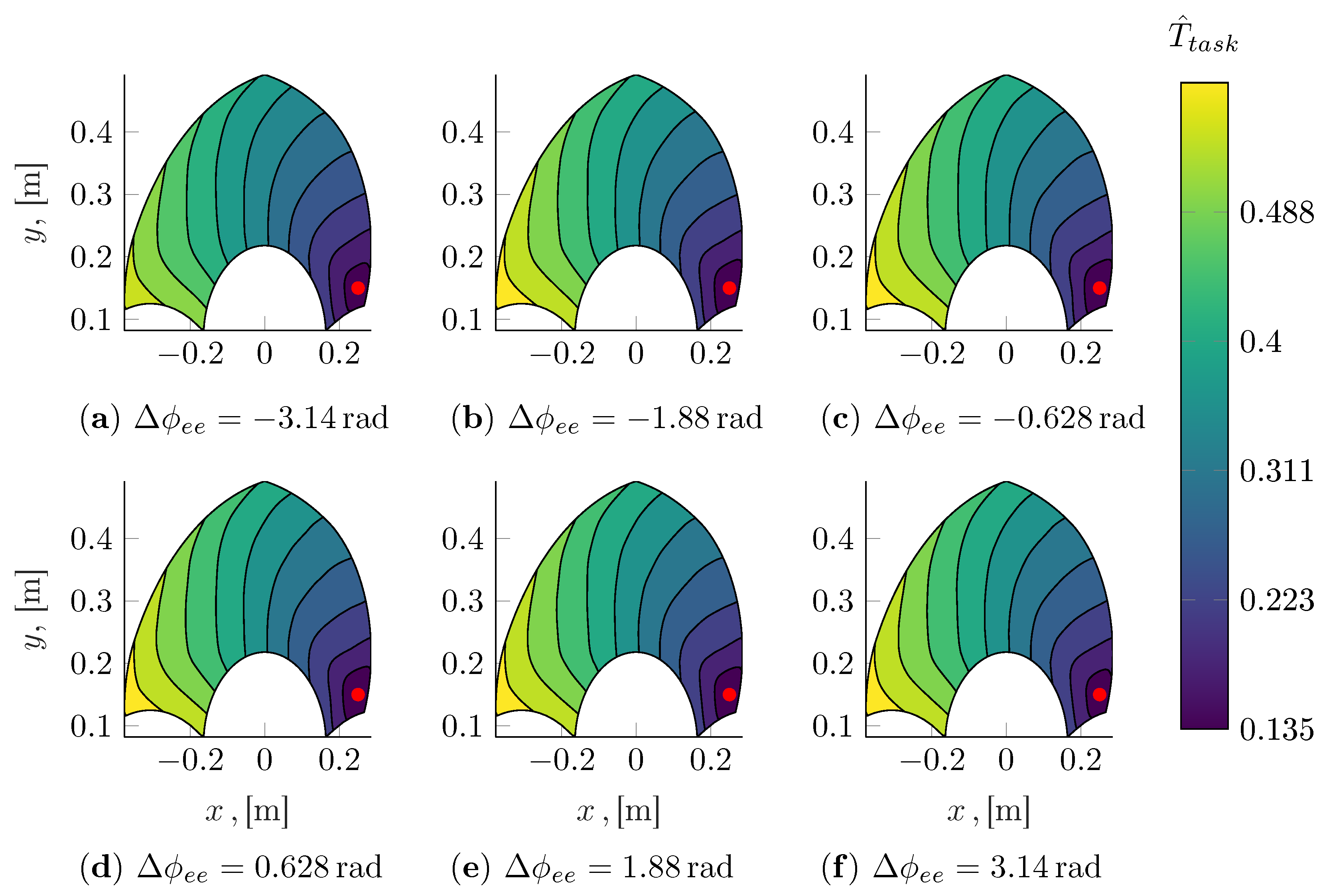
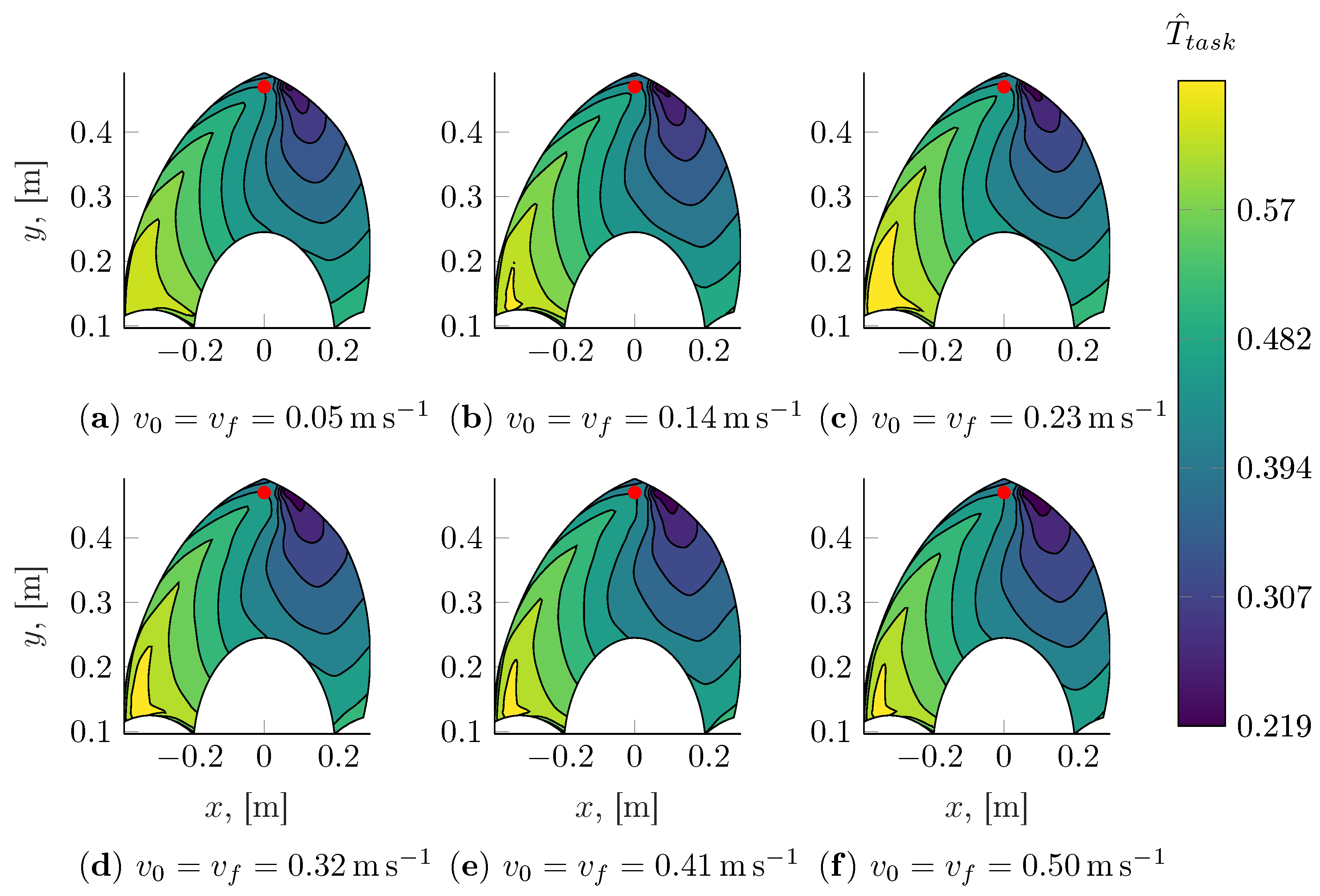
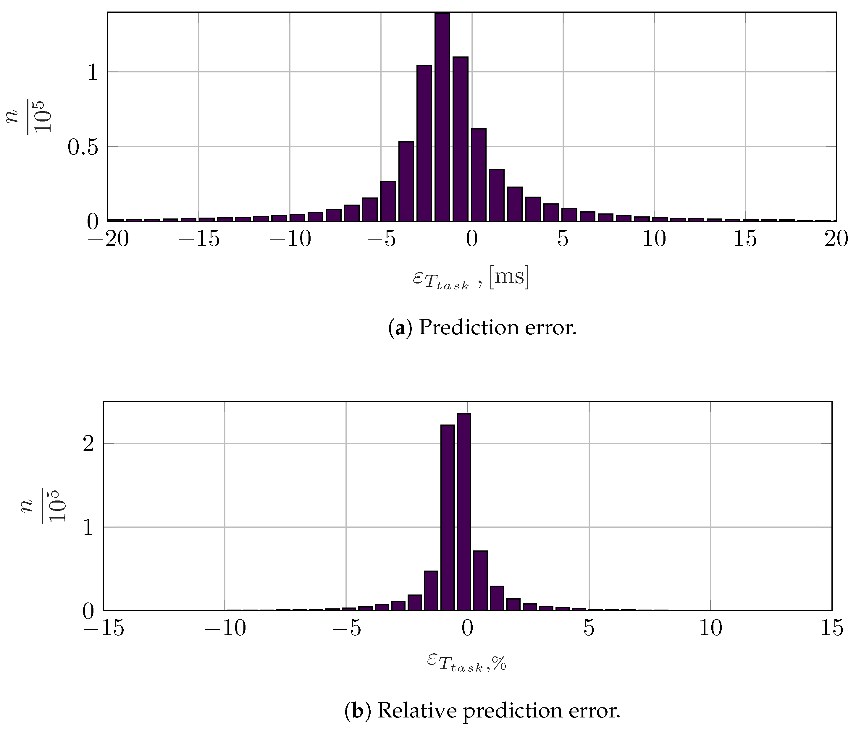
4.3. On-the-Fly Pick and Place Task Time Map

The task time map of on-the-fly pick and place operations naturally lends itself to the determination of the optimal intercept position for pick and place targets moving at a known speed profile. The need for this often arises when considering a system in which the items are picked and placed on continuously moving conveyors.

This type of planning has been illustrated qualitatively in Figure 17, which represents graphically Equation (10). In Figure 17a, the problem has been represented in the x-y plane in which the conveyor, depicted in green, is located; in the figure, the robot’s workspace (represented as a grey area) can be seen, along with the initial positions of the manipulator’s end-effector (red marker) and of the target (blue marker). As the target moves along the dotted blue line, the intercept will necessarily happen on a point belonging to it, with a final end-effector orientation and velocity (not depicted for simplicity) also dictated by the configuration of the target. The determination of the optimal intercept point is performed as shown in Figure 17b, where the time-displacement functions of the target and of the robot are displayed. The target function is a line, since its velocity is constant; on the other hand, the robot’s function can be obtained from the evaluation of the task time map. The optimal intercept position is at the intersection of these two functions, as the operation can happen as fast as possible and without having to wait for the target. When an intersection is not present, it might mean that the robot cannot operate fast enough in order to reach the target (robot time function entirely above the target time function) or, conversely, that the robot necessarily has to wait for the target to enter the workspace (robot time function entirely below the target time function). In the first case, the operation is not feasible, while in the second, the intercept position that minimizes idle time is at the boundary of the workspace itself.

A feedforward neural network having four hidden layers was selected; the main parameters of the network are summarized in

Table 4. Main parameters of the neural network architecture used for the on-the-fly pick and place neural network model.

	Layer 1	Layer 2	Layer 3	Layer 4
Type	Fully connected	Fully connected	Fully connected	Fully connected
Activation	ReLU	ReLU	ReLU	Linear
Dropout probability	0.05	0.05	0.05	0.05
$n_{in}$	5	8192	8192	8129
$n_{out}$	8192	8192	8192	1

.

The minimum reciprocal condition number of the initial and final positions has been set to ${\delta }_{\sigma }=0.2$ so that some additional space for the turning manoeuvers is always available.

The evaluation times of the on-the-fly pick and place model are:

• ${\overline{T}}_{eval,cpu}=2.31$ ms on a single CPU core;
• ${\overline{T}}_{eval,gpu}=73.42 \mathrm{\mu s}$ on the GPU;
• ${\overline{T}}_{plan}=56.9$ ms on the CPU, using the C++ implementation of the GTP and TTO.

Figure 18, Figure 19, Figure 20 and Figure 21 show the task time maps at selected initial positions and velocity boundary conditions. As expected, then, in these figures, it is clearly shown that motions with a monotonically increasing $x_{ee}$ coordinate can be executed in a shorter amount of time. On the contrary, the turning manoeuvers required for the robot to move towards decreasing $x_{ee}$ coordinates require a significant amount of time, thus making the task time function quite dissimilar from a simple overall displacement function.

The computational burden substantially increases together with the size of the network; still, it remains competitive with respect to the full planning time of the trajectory, especially if the GPU is used to evaluate the task time map. This increase in size of the network was dictated by the need to achieve sufficient accuracy. In Figure 22, the error distributions are shown; the lower accuracy obtained with the on-the-fly pick and place task time map (as compared to the stationary pick and place model) can be attributed to the higher dimensionality of the inputs and to the more complex shape of the trajectories; still, the error distribution remains reasonably concentrated around zero and is compatible to an adequate prediction of the actual task times.

In the case of on-the-fly pick and place tasks, the calculation of the intercept point depends on map task time ${\widehat{T}}_{task}$. We can consider two possible application scenarios, as previously discussed; if the command to the robot uses the boundary conditions and the map task time ${\widehat{T}}_{task}$, the robot executes the task in the given time and, therefore, the intercept error is null. If, on the contrary, the command to the robot uses only the boundary conditions, the actual and predicted task times will be different. Considering the worst case of a maximum prediction error of 20 ms and a maximum conveyor velocity of 0.5 m s⁻¹, in this case, at the end of the intercept task, the target reaches a position different from the robot’s, with a spatial error equal to 10 mm. This might be acceptable or not according to the picked item’s geometry and size. Concerning the computational costs associated with the full planning pipeline, the following considerations can be made: Figure 13, Figure 14, Figure 15 and Figure 16 and Figure 18, Figure 19, Figure 20 and Figure 21 show that even the shortest trajectories require more than 100 ms for their execution; on the other hand, in the histogram depicted in Figure 11, it can be seen that the execution of the complete motion planning pipeline, composed of the GTP and TTO, requires practically always less than 80 ms; this result, moreover, is tuneable by acting on the parameters of the optimization routines (chiefly the number of decision variables and constraints), sacrificing, if needed, accuracy for speed. Even in the most unfortunate cases (with comparatively short trajectory execution times and relatively long planning times), it is possible to plan the next trajectory while the current one is being executed. Since the conveyors move at quasi-constant velocities, it is indeed feasible to predict the motion of the targets with reasonable accuracy in order to plan in advance the next task assigned to the robot. This kind of plan-in-advance strategy is needed in any case for the on-the-fly pick and place tasks since the robot terminates its current trajectory with a non-null velocity and therefore immediately needs a new setpoint to safely prosecute its motion. As a further benefit, this strategy makes it unnecessary to consider, during the optimal intercept computation, the calculation times. The implementation of the overall planning system here briefly delineated should therefore allow the parallel execution of the control algorithms and of the planning operations, and additionally, it should perform short-term forecasts of the pick and place targets’ states.

To highlight the usefulness of the proposed method, we show in

Table 5. Solution times for several optimal intercept problems using different methods.

Task Configuration Data	Task 1	Task 2	Task 3	Task 4
$x_{rbt,0}$, [mm]	−300	175	−300	175
$y_{rbt,0}$, [mm]	150	300	150	300
${\phi }_{rbt,0}$, [${}^{\circ }$]	0.0	0.0	0.0	0.0
$v_{rbt,0}$, [m s−1]	0.2	0.2	0.2	0.2
$x_{tgt,0}$, [mm]	−150	−150	150	150
$y_{tgt,0}$, [mm]	400	400	175	175
${\phi }_{tgt,0}$, [${}^{\circ }$]	0.0	0.0	0.0	0.0
$v_{tgt,0}$, [m s−1]	0.2	0.2	0.2	0.2
$T_{task}$ evaluations	15	15	17	12
${\widehat{T}}_{task}$ evaluations	14	15	16	11
Solution time with GTP-TTO, [ms]	869	869	985	695
Solution time with task time map (CPU), [ms]	32	34	37	25
Solution time with task time map (GPU), [ms]	1.02	1.09	1.17	0.80

the computational costs associated with the solution of a few optimal intercept problems. The problem was solved thanks to an iterative root finding algorithm applied to Equation (10) using either the task time map or the direct evaluation of the GTP and TTO. In the table, the parameters concerning four different intercept tasks are shown. It can be seen that the solution of the intercept problem using either the task time map or the actual task time function requires a similar number of function evaluations. However, the difference lies in the cost of each evaluation. It can be seen that the total solution time is in the order of several hundreds of milliseconds using the direct computation approach. On the other hand, using the task time map, the problem can be solved within a a few tens of milliseconds (using the CPU) or in roughly one millisecond (using the GPU). Without the use of the task time map, therefore, the plan-in-advance strategy described above is not feasible since the computation times would be much longer than the trajectory execution times. On the contrary, the use of task time maps leads to calculation times compatible with a real application.

5. Conclusions

The paper presents a general methodology for mapping the minimal task times of industrial manipulators whose trajectories can have an arbitrary position in the workspace. The proposed methodology uses neural network models to approximate the task time function of a generic multi-DOF robot. Moreover, the work proposes a complete simulation-based workflow for determining the data needed to train the neural network that considers the manipulator’s non-linear kinematics and dynamics and the actuation system’s properties.

The neural network proposed for the task time mapping can be also trained using a different set of data with respect to those proposed by the authors. For instance, the data can be collected from simulations performed in the manufacturer’s software environment or by the experimental measure of the task time obtained by a robot that executes a comprehensive set of trajectories from and to any points belonging to the workspace. The proposed workflow is however cheaper and does not require the setup of the experimental investigation, also introducing considerable time saving. The workflow presented for determining the training data considers trajectory optimization and advanced motion planning along it and is able to satisfy stationary and on-the-fly pick and place robot jobs. The paper presents these topics both theoretically and numerically.

The results show that the evaluation of the presented task time map is 600 to 8000 times faster than the direct use of the GTP-TTO algorithm. In more complex cases dealing with on-the-fly pick and place, the task time map evaluation is 20 to 780 times faster than the direct computational effort.

Even without specialized hardware, compared with the direct evaluation of the task times, the neural network model offers significant, orders-of-magnitude speedups, which can be further increased through the use of standard GPU computing or, if needed by more demanding applications, with dedicated AI hardware accelerators. Therefore, the neural network model has been found remarkably advantageous in terms of accuracy, computational efficiency, adaptability to diverse applications, and ease of deployment; the methodology proposed by the authors is therefore shown to be suitable for scheduling strategies requiring real-time evaluation of the minimal task time. Neural networks are demonstrated to constitute a convenient architecture for implementing the task time model, as they are inherently mesh-free and more readily scalable (unlike more traditional lookup tables). The case study here proposed can be immediately adapted to a wide array of practically relevant industrial processes, namely all those plants that feature straight conveyor belts and 4-DOF manipulators such as SCARA, Clavel Delta, linear Delta, palletizing, Adept Quattro, and Cartesian robots. In cases characterized by a higher number of degrees of freedom, we expect that the dimensions of the neural network would increase. For example, a similar application with pick and place operations also requiring general spatial rotations would involve a larger number of input parameters to be fed into the neural network; it can be anticipated that the training and use of the task time models would be more expensive; the overall approach would remain however unchanged. Indeed, the neural network models are easily applied to different robots and tasks while keeping a uniform software interface. In addition, composite or hierarchical tasks, such as the shown on-the-fly pick and place operations, can be treated using the proposed methodology through the mapping of each subtask time.

Application to an industrial robot would require the use of the motion planning strategies implemented by its manufacturer, both for the generation of the task time map and in general for the utilization of the manipulator. The core of this work, namely the method for task time mapping, would still be applicable. In particular, if the motion planning strategy is unknown, the method is applicable using a task time dataset generated through experimental execution of a sufficiently exhaustive set of trajectories.

As a future work, the authors are planning to experimentally validate the developed methodology on the actual manipulator, whose open architecture makes it straightforward to apply the techniques as here described.

Another prosecution of this research is related to the possibility of completely substituting the GTP and the TTO with a neural network that outputs the entire motion profile.

Finally, an additional future work will concern the application of the proposed method to a simulated multirobot plant, with a greater focus on the productivity advantages that can be obtained thanks to scheduling algorithms based on the task time map.

References

1. Daoud, S.; Chehade, H.; Yalaoui, F.; Amodeo, L. Solving a robotic assembly line balancing problem using efficient hybrid methods. J. Heuristics 2014, 20, 235–259. [Google Scholar] [CrossRef]
2. Humbert, G.; Pham, M.T.; Brun, X.; Guillemot, M.; Noterman, D. Comparative analysis of pick & place strategies for a multi-robot application. In Proceedings of the 2015 IEEE 20th Conference on Emerging Technologies & Factory Automation (ETFA), Luxembourg, 8–11 September 2015; pp. 1–8. [Google Scholar]
3. Humbert, G.; Brun, X.; Pham, M.T.; Guillemot, M.; Noterman, D. Development of a methodology to improve the performance of multi-robot pick & place applications: From simulation to experimentation. In Proceedings of the 2016 IEEE International Conference on Industrial Technology (ICIT), Taipei, Taiwan, 14–17 March 2016; pp. 1960–1965. [Google Scholar]
4. Ferrari, G.; Ferrarini, L.; Petretti, A.; Pizzi, E. Modeling and design of an optimal line manager of a packaging system with MILP. In Proceedings of the IECON 2015—41st Annual Conference of the IEEE Industrial Electronics Society, Yokohama, Japan, 9–12 November 2015; pp. 005050–005056. [Google Scholar]
5. Pizzi, E.; Bouchrit, A.; Petretti, A.; Ferrarini, L. Performance improvement for online schedulers for packaging systems. In Proceedings of the 2016 IEEE International Conference on Automation Science and Engineering (CASE), Fort Worth, TX, USA, 21–24 August 2016; pp. 1243–1248. [Google Scholar]
6. Wang, P.; Ma, H.; Zhang, Y.; Cao, X.; Wu, X.; Wei, X.; Zhou, W. Trajectory Planning for Coal Gangue Sorting Robot Tracking Fast-Mass Target under Multiple Constraints. Sensors 2023, 23, 4412. [Google Scholar] [CrossRef] [PubMed]
7. Wilson, D.B.; Soto, M.A.T.; Goktogan, A.H.; Sukkarieh, S. Real-time rendezvous point selection for a nonholonomic vehicle. Proceedings of 2013 IEEE International Conference on Robotics and Automation, Karlsruhe, Germany, 6–10 May 2013; pp. 3941–3946. [Google Scholar] [CrossRef]
8. Shin, I.S.; Nam, S.H.; Roberts, R.; Moon, S. A minimum-time algorithm for intercepting an object on a conveyor belt. Ind. Robot. 2009, 36, 127–137. [Google Scholar] [CrossRef]
9. Croft, E.A.; Fenton, R.G.; Benhabib, B. An on-line robot planning strategy for target interception. J. Robot. Syst. 1998, 15, 97–114. [Google Scholar] [CrossRef]
10. Jasour, A.M.; Farrokhi, M. Adaptive neuro-predictive control for redundant robot manipulators in presence of static and dynamic obstacles: A Lyapunov-based approach. Int. J. Adapt. Control Signal Process. 2014, 28, 386–411. [Google Scholar] [CrossRef]
11. Han, S.D.; Feng, S.W.; Yu, J. Toward fast and optimal robotic pick-and-place on a moving conveyor. IEEE Robot. Autom. Lett. 2019, 5, 446–453. [Google Scholar] [CrossRef]
12. Kröger, T. Opening the door to new sensor-based robot applications—The Reflexxes Motion Libraries. In Proceedings of the 2011 IEEE International Conference on Robotics and Automation, Shanghai, China, 9–13 May 2011; pp. 1–4. [Google Scholar]
13. Mattone, R.; Divona, M.; Wolf, A. Sorting of items on a moving conveyor belt. Part 2: Performance evaluation and optimization of pick-and-place operations. Robot.-Comput.-Integr. Manuf. 2000, 16, 81–90. [Google Scholar] [CrossRef]
14. Boschetti, G. A picking strategy for circular conveyor tracking. J. Intell. Robot. Syst. 2016, 81, 241–255. [Google Scholar] [CrossRef]
15. Zhou, M.; Jiang, R. Optimal Strategy for Pick-and-Place System with two Robots. J. Phys. 2022, 2216, 012022. [Google Scholar] [CrossRef]
16. Scalera, L.; Boscariol, P.; Carabin, G.; Vidoni, R.; Gasparetto, A. Enhancing energy efficiency of a 4-DOF parallel robot through task-related analysis. Machines 2020, 8, 10. [Google Scholar] [CrossRef]
17. Bobrow, J.E.; Dubowsky, S.; Gibson, J.S. Time-optimal control of robotic manipulators along specified paths. Int. J. Robot. Res. 1985, 4, 3–17. [Google Scholar] [CrossRef]
18. Pham, Q.C.; Stasse, O. Time-optimal path parameterization for redundantly actuated robots: A numerical integration approach. IEEE/ASME Trans. Mechatronics 2015, 20, 3257–3263. [Google Scholar] [CrossRef]
19. Pham, H.; Pham, Q.C. Time-optimal path tracking via reachability analysis. In Proceedings of the 2018 IEEE International Conference on Robotics and Automation (ICRA), Brisbane, Australia, 21–25 May 2018; pp. 3007–3012. [Google Scholar]
20. Verscheure, D.; Demeulenäre, B.; Swevers, J.; De Schutter, J.; Diehl, M. Practical time-optimal trajectory planning for robots: A convex optimization approach. IEEE Trans. Autom. Control 2008, 53, 28. [Google Scholar]
21. Pham, H.; Pham, Q.C. On the structure of the time-optimal path parameterization problem with third-order constraints. In Proceedings of the 2017 IEEE International Conference on Robotics and Automation (ICRA), Singapore, 29 May–3 June 2017; pp. 679–686. [Google Scholar]
22. Fan, W.; Gao, X.S.; Lee, C.H.; Zhang, K.; Zhang, Q. Time-optimal interpolation for five-axis CNC machining along parametric tool path based on linear programming. Int. J. Adv. Manuf. Technol. 2013, 69, 1373–1388. [Google Scholar] [CrossRef]
23. Zhang, Q.; Li, S.R.; Gao, X.S. Practical smooth minimum time trajectory planning for path following robotic manipulators. In Proceedings of the 2013 American Control Conference, Washington, DC, USA, 17–19 June 2013; pp. 2778–2783. [Google Scholar]
24. Gasparetto, A.; Boscariol, P.; Lanzutti, A.; Vidoni, R. Path planning and trajectory planning algorithms: A general overview. Motion Oper. Plan. Robot. Syst. Backgr. Pract. Approaches 2015, 2015, 3–27. [Google Scholar]
25. Braghin, F.; Cheli, F.; Melzi, S.; Sabbioni, E. Race driver model. Comput. Struct. 2008, 86, 1503–1516. [Google Scholar] [CrossRef]
26. Sabelhaus, D.; Röben, F.; zu Helligen, L.P.M.; Lammers, P.S. Using continuous-curvature paths to generate feasible headland turn manoeuvres. Biosyst. Eng. 2013, 116, 399–409. [Google Scholar] [CrossRef]
27. Zhao, H.; Zhu, L.; Ding, H. A real-time look-ahead interpolation methodology with curvature-continuous B-spline transition scheme for CNC machining of short line segments. Int. J. Mach. Tools Manuf. 2013, 65, 88–98. [Google Scholar] [CrossRef]
28. Tang, P.Y.; Lin, M.T.; Tsai, M.S.; Cheng, C.C. Toolpath interpolation with novel corner smoothing technique. Robot. Comput. Integr. Manuf. 2022, 78, 102388. [Google Scholar] [CrossRef]
29. Chen, G.; Luo, N.; Liu, D.; Zhao, Z.; Liang, C. Path planning for manipulators based on an improved probabilistic roadmap method. Robot. Comput. Integr. Manuf. 2021, 72, 102196. [Google Scholar] [CrossRef]
30. Righettini, P.; Strada, R.; Zappa, B.; Lorenzi, V. Experimental set-up for the investigation of transmissions effects on the dynamic performances of a linear PKM. In Proceedings of the Advances in Mechanism and Machine Science: Proceedings of the 15th IFToMM World Congress on Mechanism and Machine Science 15, Krakow, Poland, 30 June–4 July 2019; pp. 2511–2520. [Google Scholar]
31. Righettini, P.; Strada, R.; Cortinovis, F. Modal kinematic analysis of a parallel kinematic robot with low-stiffness transmissions. Robotics 2021, 10, 132. [Google Scholar] [CrossRef]
32. Righettini, P.; Strada, R.; Cortinovis, F. General Procedure for Servo-Axis Design in Multi-Degree-of-Freedom Machinery Subject to Mixed Loads. Machines 2022, 10, 454. [Google Scholar] [CrossRef]
33. Bourbonnais, F.; Bigras, P.; Bonev, I.A. Minimum-time trajectory planning and control of a pick-and-place five-bar parallel robot. IEEE/ASME Trans. Mechatronics 2014, 20, 740–749. [Google Scholar] [CrossRef]
34. Yu, H. Modeling and control of hybrid machine systems—A five-bar mechanism case. Int. J. Autom. Comput. 2006, 3, 235–243. [Google Scholar] [CrossRef]
35. Stellato, B.; Banjac, G.; Goulart, P.; Bemporad, A.; Boyd, S. OSQP: An operator splitting solver for quadratic programs. Math. Program. Comput. 2020, 12, 637–672. [Google Scholar] [CrossRef]
36. Takahasi, H.; Mori, M. Double exponential formulas for numerical integration. Publ. Res. Inst. Math. Sci. 1974, 9, 721–741. [Google Scholar] [CrossRef]
Figure 1. Schematic representation of a non-deterministic and time-constrained on-the-fly manipulation task.
Robotics 12 00143 g001
Figure 2. Pictorial representation of the scheduling, geometric motion planning, and task time optimization pipeline.
Robotics 12 00143 g002
Figure 3. Input–output representation of the scheduling, geometric motion planning, and task time optimization pipeline.
Robotics 12 00143 g003
Figure 4. Statistical comparison between the trajectory execution times obtained through convex optimization and linear programming.
Robotics 12 00143 g004
Figure 5. Conceptual diagram of the training process of the task time model; p s , p f , v s , and v f represent the position and velocity boundary conditions of the trajectory, while T t a s k and T ^ t a s k denote each the actual task time of the trajectory and its estimation.
Robotics 12 00143 g005
Figure 6. 5R manipulator at the University of Bergamo and schematic representation of its actuation and transmission systems.
Robotics 12 00143 g006
Figure 7. Notable points and angular quantities of the 5R planar linkage.
Robotics 12 00143 g007
Figure 8. Reciprocal condition number represented in the admissible portions of the workspace.
Robotics 12 00143 g008
Figure 9. Examples of a composite trajectory for on-the-fly pick and place.
Robotics 12 00143 g009
Figure 10. Examples of point-to-point paths (a), tracking paths (b), and paths for stationary pick and place tasks (c).
Robotics 12 00143 g010
Figure 11. Histogram of measured planning times.
Robotics 12 00143 g011
Figure 12. Stationary pick and place task time prediction errors calculated on the test dataset.
Robotics 12 00143 g012
Figure 13. Stationary pick and place task time model evaluated at different end-effector rotational displacements Δ ϕ e e ; the initial configuration of the robot, shown as a red marker, has been fixed at x e e = 0.0   m , y e e = 0.25   m .
Robotics 12 00143 g013
Figure 14. Stationary pick and place task time model evaluated at different end-effector rotational displacements Δ ϕ e e ; the initial configuration of the robot, shown as a red marker, has been fixed at x e e = 0.25   m , y e e = 0.15   m .
Robotics 12 00143 g014
Figure 15. Stationary pick and place task time model evaluated at different end-effector rotational displacements Δ ϕ e e ; the initial configuration of the robot, shown as a red marker, has been fixed at x e e = 0.25   m , y e e = 0.15   m .
Robotics 12 00143 g015
Figure 16. Stationary pick and place task time model evaluated at different end-effector rotational displacements Δ ϕ e e ; the initial configuration of the robot, shown as a red marker, has been fixed at x e e = 0.0   m , y e e = 0.47   m .
Robotics 12 00143 g016
Figure 17. Graphical representation of an optimal intercept position computation.
Robotics 12 00143 g017
Figure 18. On-the-fly pick and place task time model evaluated for different end-effector initial and final velocities v 0 and v f ; the initial configuration of the robot, shown as a red marker, has been fixed at x e e = 0.0   m , y e e = 0.25   m .
Robotics 12 00143 g018
Figure 19. On-the-fly pick and place task time model evaluated for different end-effector initial and final velocities v 0 and v f ; the initial configuration of the robot, shown as a red marker, has been fixed at x e e = 0.25   m , y e e = 0.15   m .
Robotics 12 00143 g019
Figure 20. On-the-fly pick and place task time model evaluated for different end-effector initial and final velocities v 0 and v f ; the initial configuration of the robot, shown as a red marker, has been fixed at x e e = 0.25   m , y e e = 0.15   m .
Robotics 12 00143 g020
Figure 21. On-the-fly pick and place task time model evaluated for different end-effector initial and final velocities v 0 and v f ; the initial configuration of the robot, shown as a red marker, has been fixed at x e e = 0.0   m , y e e = 0.47   m .
Robotics 12 00143 g021
Figure 22. On-the-fly pick and place task time prediction errors calculated on the test dataset.
Robotics 12 00143 g022