Article

Adaptive Backstepping Integral Sliding Mode Control of a MIMO Separately Excited DC Motor

1
Department of Electrical and Computer Engineering, COMSATS University, Islamabad 45550, Pakistan
2
Department of Electrical and Computer Engineering, International Islamic University, Islamabad 44000, Pakistan
3
School of Computer Science, Faculty of Science and Engineering, University of Hull, Kingston upon Hull HU6 7RX, UK
*
Author to whom correspondence should be addressed.
Robotics 2023, 12(4), 105; https://doi.org/10.3390/robotics12040105
Submission received: 30 May 2023 / Revised: 5 July 2023 / Accepted: 10 July 2023 / Published: 16 July 2023
(This article belongs to the Special Issue New Trends in Robotics and Mechatronic Technologies)

Abstract

:
This research proposes a robust nonlinear hybrid control approach to the speed control of a multi-input-and-multi-output separately excited DC motor (SEDCM). The motor that was under consideration experienced parametric uncertainties and load disturbances in the weak field region. The proposed technique aims to merge the benefits of adaptive backstepping (AB) and integral sliding mode control (ISMC) to enhance the overall system’s robustness. The unknown parameters with load disturbances are estimated using an adaptation law. These estimated parameters are incorporated into the controller design, to achieve a highly robust controller. The theoretical stability of the system is proved using the Lyapunov stability criteria. The effectiveness of the proposed AB–ISMC was demonstrated by simulation, to track the reference speed under parametric uncertainties and load disturbances. The control performance of the proposed technique was compared to that of feedback linearization (FBL), conventional sliding mode control (SMC), and AB control laws without and with the adaptation law. Regression parameters, such as integral square error, integral absolute error, and integral time absolute error, were calculated to quantitatively analyze the tracking performance and robustness of the implemented nonlinear control techniques. The simulation results demonstrated that the proposed controller could accurately track the reference speed and exhibited robustness, with steady-state error accuracy. Moreover, AB–ISMC overperformed, compared to the FBL, SMC, AB controller without adaptation law and AB controller with adaptation law, in reducing the settling time by factors of 27 % , 67 % , 23 % , and 21 % , respectively, thus highlighting the superior performance of the proposed controller.

1. Introduction

Electrical devices play a vital role in control systems and robotics [1]. A common type of electrical device used in various industrial areas is the DC motor, which converts electrical energy to mechanical energy. DC motors offer numerous advantages, such as the ability to control continuous and instantaneous speed [2,3]. These merits make them versatile for diverse applications, including electric vehicles, pumps, home appliances, electric cranes, steel rolling mills, and robotic manipulators [1,3].
In recent years, separately excited DC machines have gained significant popularity for variable speed applications, due to their controllability and ease of use [3]. However, the dynamic model of a separately excited DC motor (SEDCM) operating in the weak field region is highly nonlinear. The term “weak field region” refers to a specific operating region of a SEDCM, where the magnetic field strength produced by the field winding is relatively weak. This weakening of the magnetic field allows the motor to operate at higher speeds than its rated speed. For carrying out a variety of tasks, a machine operates at different speed modes. Therefore, it needs a controller that can adjust and control its speed according to the specific application requirement [4]. Furthermore, accurate modeling and control of the system becomes challenging, due to the varying system parameters and complex system dynamics [5,6].
There exist several solutions for the speed control of a SEDCM. Classical controllers find extensive application in the speed control of a SEDCM due to their suitability and wide acceptance. The accuracy of the mathematical model of the system is a crucial factor in determining the performance of these controllers in various industrial applications [7]. Developing mathematical models that account for parameter variations is essential for achieving reliable controller performance. Proportional–integral–derivative (PID) controllers are widely used to control the speed of a SEDCM above the base speed, because of their simplicity and ease of implementation. However, at high speed, the effectiveness of the PID controller tends to deteriorate, due to the significant nonlinearities observed in the motor’s behavior, particularly in the weak field region [3,6,8,9,10]. In [6], a PID controller using the artificial bee colony (ABC) algorithm was proposed, to enhance the speed control of a motor. In [8], speed control of a SEDCM using a DC–DC converter and control strategies, like proportional–integral (PI) control and fuzzy logic, were used to minimize speed control errors. Research reported in [9] presented the utilization of PI and fuzzy logic controllers (FLC) for speed control of a SEDCM. The research work [11,12] introduced a sensorless control system and an adaptive load approach to improve motor performance, proposing the online tuning of PID controller parameters through the recursive least square algorithm.
Conventional controllers struggle to maintain a constant speed for the motor, due to parametric variations associated with nonlinear loads, such as friction and magnetic saturation [13]. PI and PID controllers, commonly used for speed control, require continuous tuning of control parameters, posing a challenging task during operation. On the other hand, fuzzy controllers are highly versatile and widely employed for speed control in industrial and domestic applications. However, fuzzy controllers rely on selecting appropriate values for membership functions, which is crucial for their effective functioning. As a result, researchers have been exploring various new control techniques to enhance the system’s performance. Nonlinear control techniques, such as feedback linearization (FBL), sliding mode control (SMC), and backstepping control (BSC), have been proposed and applied, to control the speed of a SEDCM above base speed [3,10,14]. These controllers can handle the nonlinearities in the behavior of the motor more effectively than PID controllers, resulting in better performance in the weak field region [3,15,16].
A study conducted in [14] investigated the nonlinear behavior of a DC motor and proposed an FBL control approach, using a metaheuristic optimization algorithm for improved performance. Research reported in [17] focused on designing and analyzing a partial FBL controller for AC and DC machines. The simplicity of the FBL approach has made it a popular choice among nonlinear control techniques for controlling nonlinear systems: it involves transforming the nonlinear system dynamics into a linear one, which allows for the use of linear control methods. However, the performance of the FBL approach may deteriorate, due to the parametric variations and load disturbances [17,18].
To tackle these challenges, researchers have utilized sliding mode algorithms, to attain robust control over motor speed. SMC is an effective control technique that can yield outstanding performance, despite uncertainties and disturbances. However, the main drawback of SMC is chattering, which is typically undesirable in practical drive systems [18,19,20,21,22,23,24]. The research in [18] introduced an integral sliding mode control (ISMC) method for starting induction motors (IM) in the rotating condition without a speed sensor. The ISMC method, utilizing the rotor’s back electromotive force model, ensures precise and rapid estimation of the initial speed. Stability and robustness are analyzed using Lyapunov stability criteria. Compared to the existing input–output feedback linearization (IOFL) control method, the proposed approach exhibits improved dynamic performance, robustness, and absence of overshooting during speed estimation. The work reported in [19] explores the implementation of SMC for speed control of permanent magnet synchronous motors (PMSMs). The study investigated different sliding surfaces and composite controller designs to enhance the robustness of the controller and reduce chattering in a SMC-based law with a particular focus on the use of a fractional-order sliding surface design. The simulation results validated the effectiveness of the proposed fractional-order SMC (FOSMC) law for robust and precise speed regulation of PMSM. The introduced sliding surface design enhanced FOSMC by reducing torque ripple, chattering, and improving anti-disturbance properties compared to FOSMC with PI or proportional–derivative (PD) sliding surfaces. In [25], a comparative analysis revealed that the AB super-twisting SMC-based control law demonstrated superior performance in terms of cyclic path tracking and disturbance rejection. The control community has consistently improved SMC techniques to enhance their effectiveness in nonlinear systems. These controllers have good tracking performance and can effectively handle disturbances. However, a significant drawback of SMC is the chattering effect, which adversely impacts its overall performance [21,22].
The BSC algorithm is a nonlinear technique that offers a systematic approach for designing a control law to track a desired reference signal by selecting an appropriate Lyapunov function. Despite its effectiveness, BSC may not be robust enough to handle parametric uncertainties [3,20,21,22]. Unlike SMC, BSC does not suffer from the chattering effect. However, its ability to effectively reject disturbances caused by load torque is relatively less efficient than SMC [26].
A SEDCM plays a pivotal role in several industrial and domestic applications, particularly where precise speed control is required. However, classical controllers encounter difficulties when it comes to managing load changes in the motor. Controlling the motor’s speed under varying loads poses a great challenge, making it a complex task to maintain a steady-state condition. To achieve speeds beyond the base speed, a SEDCM utilizes a field-weakening control technique. However, its operation in the weak field region introduces nonlinearities in the motor’s model, primarily due to back EMF and electromagnetic torque. Thus, designing a robust controller to effectively mitigate nonlinearities, uncertainties, and load torque disturbances in a SEDCM poses a significant challenge, especially when aiming for superior dynamic performance. Various control techniques have been explored to address the challenge of speed tracking. The primary goal of a speed controller is to achieve the desired motor speed accurately. Additionally, conducting a comprehensive performance comparison among various nonlinear control techniques is important to identify the most suitable approach for a specific application.
The present research proposes an adaptive backstepping integral sliding mode controller (AB–ISMC) to address the aforementioned shortcomings and to enhance the system performance. The controller design improves the tracking of the reference signals in the presence of parametric uncertainties and load disturbances. The AB–ISMC aims to enhance the control system’s performance by reducing chattering, improving settling time, and decreasing the steady-state error. The proposed controller enhances the overall robustness and ensures system stability based on Lyapunov stability criteria. The designed control technique is applied to control the speed of a SEDCM in the weak field region. The results indicate that the proposed hybrid controller outperforms compared to FBL, SMC, and AB strategies by effectively reducing steady-state error and improving settling time.
The rest of the paper is organized as follows: Section 2 presents the model of a SEDCM. The design methodologies of various nonlinear control techniques including FBL, SMC, AB (case 1 and case 2), and AB–ISMC, are discussed in Section 3. The simulation results are presented in Section 4. Finally, Section 5 summarizes the conclusions drawn from the study and highlights potential areas for future research.

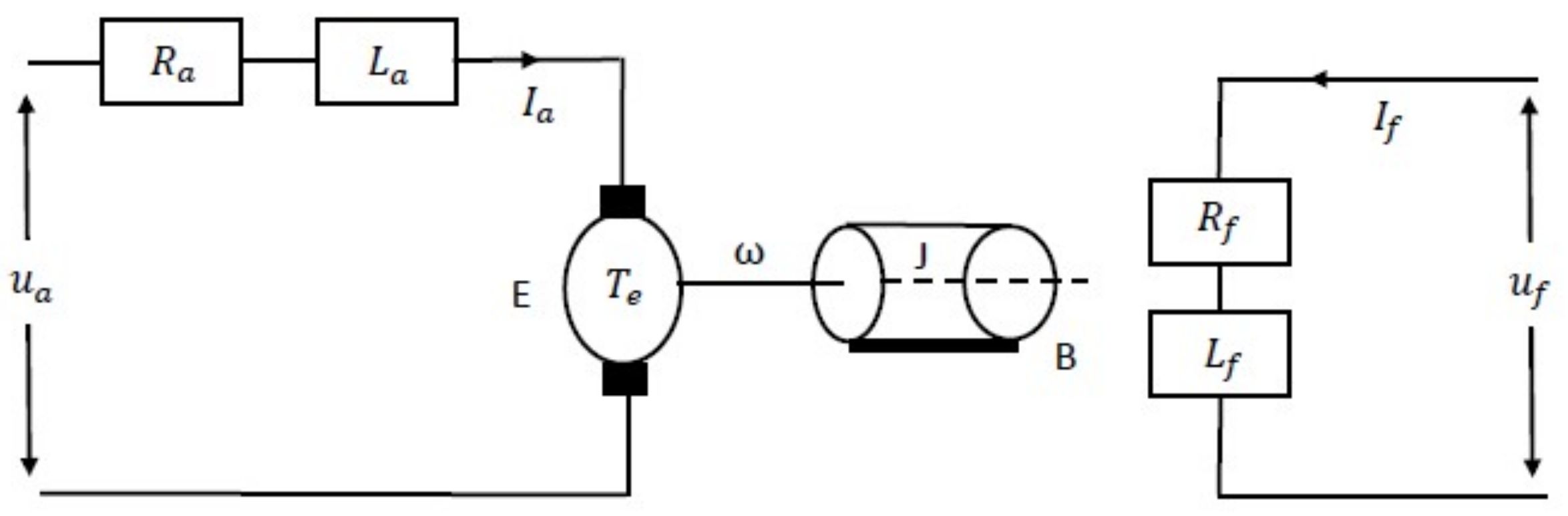
2. Mathematical Model of a SEDCM

The SEDCM shown in Figure 1 is a common type of DC motor that consists of a separate field and an armature winding, each with its own voltage source. This enables the armature voltage and the field voltage to be used as control inputs, allowing for precise control of the motor’s speed [3]. The parameters of the SEDCM used in the simulation are given in Table 1.
Assuming a linear magnetization curve in which the flux is not saturated, the relationship between the flux and the field current can be expressed as φ = L f I f , where L f represents the field inductance. The state vector is defined as x = [ x 1 x 2 x 3 ] T = [ I a I f w ] T . Based on this assumption, the equations for a SEDCM can be written as follows:
d I a d t = 1 L a ( u a R a I a E ) d I f d t = 1 L f ( u f R f I f ) d w d t = 1 J ( T e B w T L )
where E = K I f w and T e = K I f I a . The symbol E represents the back EMF, while T e represents the electric torque. The armature current and field current are represented by I a and I f , respectively.
Equation (1) presents a general model of a SEDCM that involves armature voltage and field circuit voltage as control inputs. The presence of terms like K I f w and K I f I a makes this model highly nonlinear. These nonlinearities can significantly affect the performance of the motor in the weak field region, which requires precise control. Therefore, a nonlinear controller should be designed to compensate for the nonlinearities. To simplify computation, the following constants are defined.
a 1 = R a L a , a 2 = K L a , a 3 = R f L f , a 4 = K J , a 5 = B J
Therefore, (1) can be written as,
x ˙ 1 = a 1 x 1 + a 2 x 2 x 3 + u a L a x ˙ 2 = a 3 x 2 + u f L f x ˙ 3 = a 4 x 1 x 2 + a 5 x 3 T L J
where the states x 1 , x 2 and x 3 , respectively, correspond to I a , I f and w.

3. Nonlinear Controllers Design

Various nonlinear controllers are developed in the present research to address the challenges of robustness and speed tracking of a SEDCM. These controllers are described in the following section.
Equation (1) can be expressed in a more concise form as follows:
x ˙ = f ( x ) + g a u a + g f u f
where g a = [ 1 L a 0 0 ] T , g f = [ 0 1 L f 0 ] T , f ( x ) = 1 L a ( E R a I a ) 1 L f R f I f 1 J ( T e B w T L )

3.1. Feedback Linearization (FBL) Based Control

FBL is a widely used nonlinear control technique for DC motors. Its fundamental concept involves converting the nonlinear system into a linear system via a coordinate transformation. This transformation can be achieved by selecting a suitable state transformation function that maps the nonlinear state variables to new linear ones [24,27]. A mathematical transformation is employed in this research to facilitate the design of control schemes for speed control of a SEDCM using FBL. This transformation allows the system (3) to be expressed in a more convenient form. This is achieved by involving a change of variables that can simplify the equations and make them easier to work with.
Consider the following change of variables:
ζ 1 = x 3 ζ 2 = a 4 x 1 x 2 + a 5 x 3 T L J ζ 3 = x 2
For ζ 3 0 , the inverse transformation of the new variables is given as
x 1 = 1 a 4 ζ 3 ( ζ 2 a 5 ζ 1 + T L J ) x 2 = ζ 3 x 3 = ζ 1
Therefore, the equations of SEDCM can be written as functions of the new variables ζ 1 , ζ 2 , ζ 3 , and the inputs u 1 , u 2 . Such that
ζ ˙ 1 = ζ 2 ζ ˙ 2 = ( a 1 a 5 + a 3 a 5 ) ζ 1 + ( a 1 + a 3 + a 5 ) ζ 2 ( a 1 + a 3 + a 5 ) T L J + a 2 a 4 ζ 1 ζ 3 2 + u 1 ζ ˙ 3 = a 3 ζ 3 + u 2
Among them,
u 1 = a 4 L a x 2 u a + a 4 L f x 1 u f u 2 = 1 L f u f
To achieve precise speed control for a SEDCM, it is necessary to ensure that the speed tracking error is zero, meaning that the motor’s speed exactly follows the reference speed in a steady-state. Therefore, an error tracking control signal ( e ) is defined as follows:
e = ζ ζ d
where,
ζ d = ζ 1 d ζ 2 d ζ 3 d = w r e f 0 I f r e f
Let the system reference input be r = [ r 1 r 2 ] T , such that
A ζ d + B r = 0
where r is the reference model.
r = r 1 r 2 = ( R a L a + R f L f ) B J w r e f R f L f I f r e f
Equation (6) can be written in a compact form as
ζ ˙ = A ζ + B f ¯ + B u + z
where,
A = 0 1 0 ( a 1 + a 3 ) a 5 a 1 + a 3 + a 5 0 0 0 a 3 , ζ = ζ 1 ζ 2 ζ 3
B = 0 0 1 0 0 1 , f ¯ = a 2 a 4 ζ 1 ζ 3 2 0 , u = u 1 u 2 , z = 0 ( a 1 + a 3 + a 5 ) T L J 0
Remark 1.
It is assumed that nonlinear term f ¯ is bounded by a known function β such that
| | f ¯ | | = a 2 a 4 ζ 1 ζ 3 2 β
The final feedback linearization control law is as follows:
u = f ¯ k e + r
where k is the controller gain.

3.2. Design of Sliding Mode Controller

SMC is a robust nonlinear control technique that is useful to control dynamic systems subjected to uncertainties and disturbances. SMC achieves control by creating a sliding surface in the state space that drives the system toward the desired state trajectory. During the analysis of the system’s response in SMC, there are two distinct phases: (i) the sliding phase and (ii) the reaching phase [20,28,29]. For the design of SMC for a SEDCM, the sliding surface is designed to force the output trajectory y to follow a reference y r e f . Thus, S ( x , t ) can be chosen as
S j ( x , t ) = i = 0 r j 1 l j i ( y j r e f y j ) ( i ) j = 1 , 2 , . . . m
The relative degree r j determines the dependency of S j on S ˙ . By selecting suitable coefficients l j i , the system dynamics can be maintained onto the sliding surface, ensuring that it moves toward the origin and reduces the tracking error ( y r e f y ) when constrained to stay on the surface S ( x , t ) = 0 . According to (15), the sliding surfaces are designed as,
S 1 = l 10 ( x 3 r e f x 3 ) + l 11 ( x ˙ 3 r e f x ˙ 3 ) S 2 = l 20 ( x 2 r e f x 2 )
The objective is to force the outputs to reach the sliding surface. By solving (16), the control law is designed as
u a u f = u 11 + u 12 u 22
where,
u 11 = a 11 ( x ) + k 1 s i g n ( S 1 ) b 11 ( x ) u 12 = b 12 [ a 22 ( x ) + k 2 s i g n ( S 2 ) ] b 11 ( x ) b 21 ( x ) u 22 = a 22 ( x ) + k 2 s i g n ( S 2 ) b 21 ( x )
where k j and l j i , respectively, determine the control gain and the convergence rate when the system is in sliding mode. This control input in (17) is fed to a SEDCM to achieve the desired results and to compensate for the load disturbances.

3.3. Nonlinear Adaptive Backstepping Controller

Backstepping is a nonlinear control technique that utilizes Lyapunov functions to design a control law for nonlinear systems. It is a recursive design procedure that decomposes the n t h order nonlinear system into n scalar sub-systems. Therefore, the design procedure becomes more flexible to achieve the desired control objectives, such as stabilization or tracking. Backstepping is a popular and effective strategy for controlling nonlinear systems using Lyapunov functions [3,20,30,31].
AB technique is a variant of the BSC technique used to control nonlinear systems with unknown or time-varying parameters. The approach involves incorporating an adaptive mechanism into the backstepping design procedure, allowing the controller to adjust its parameters in response to changes in the system dynamics. The approach has been widely used in various areas, including robotics, aerospace, and power systems [3,31,32]. Its ability to handle uncertainties and adapt to changes in the system dynamics makes it well-suited for controlling complex and nonlinear systems.

Adaptive Backstepping Controller Design

The compact form of the system (1) with uncertainties can be written as follows:
x ˙ = f N ( x ) + f ( x ) + g a u a + g f u f
where f N ( x ) and f ( x ) are the nominal and uncertain matrices. The uncertainties considered in the system model are armature resistance, field resistance and load torque. These are, respectively, given as
R a = R a R a N R f = R f R f N T L = T L T L N
where R a N , R f N and T L N are the nominal values. R a , R f , T L are the uncertainties. The objective is to develop an AB controller capable of accurately monitoring the reference speed w r e f over the range w w N . The control scheme is designed to compensate for parametric uncertainties, such as R f and R a and effectively reject load disturbances. The output variables of the system are given in (21).
h 1 ( x ) = w h 2 ( x ) = I f
The notations L f h ( x ) = h . f ( x ) and L f i h ( x ) = L f ( L f i 1 h ) are used for the Lie derivative of function h ( x ) along a vector field f ( x ) and its iterative form, respectively. This change of coordinates is one-to-one in s = x R 3 : i f 0 a n d w 0 . The system in the new coordinates is given by
z ˙ 1 z ˙ 2 z ˙ 3 = z 2 L f N 2 h 1 ( x ) L f N h 2 ( x ) + L f h 1 ( x ) L f L f N h 1 ( x ) L f h 2 ( x ) + 0 0 1 0 0 1 u ^ a u ^ f
where,
u ^ a = L g a L f N h 1 ( x ) u a + L g f L f N h 1 ( x ) u f u ^ f = L g a h 2 ( x ) u a + L g f h 2 ( x ) u f
To improve the transient performance, a linear reference model is defined as
z ˙ m = A m z m + B m u r e f
z ˙ 1 m z ˙ 2 m z ˙ 3 m = 0 1 0 c 1 m c 2 m 0 0 0 c 3 m z 1 m z 2 m z 3 m + 0 0 c 1 m 0 0 c 3 m w r e f I f r e f
where c 1 m , c 2 m and c 3 m are the design parameters. The tracking error e is defined as
e = e 1 e 2 e 3 = z 1 z 1 m z 2 z 2 m z 3 z 3 m
The corresponding error dynamics are given as
e ˙ = A ( x ) + A ( x ) + B u ¯
where,
e ˙ 1 = e 2 + L f h 1 ( x )
e ˙ 2 = L f N 2 h 1 ( x ) + L f L f N h 1 ( x ) + u ¯ a
e ˙ 2 = L f N h 2 ( x ) + L f h 2 ( x ) + u ¯ f
In (27) the terms A ( x ) , A ( x ) and B u ¯ corresponds as
u ¯ = u ¯ a u ¯ f = u ^ a + c 1 m z 1 m + c 2 m z 2 m c 1 m w r e f u ^ f + c 3 m z 3 m c 3 m I f r e f
A ( x ) = e 2 L f N 2 h 1 ( x ) L f N h 2 ( x ) , B = 0 0 1 0 0 1 , A ( x ) = L f h 1 ( x ) L f L f N h 1 ( x ) L f h 2 ( x ) = ϑ 1 ϕ 1 ( x ) ϑ 2 ϕ 2 ( x ) ϑ 3 ϕ 3 ( x )
It is assumed that ϑ 1 , ϑ 2 and ϑ 3 in (27) are unknown uncertainties. By careful examination of (27), it can be observed that the error-tracking model of the SEDCM contains two decoupled sub-systems. The first sub-system consists of (27a) and (27b) and is controlled by u ¯ a , while the second sub-system, which is (27c), is controlled by u ¯ f . This structural property allows the appropriate use of the AB design technique to obtain the desired controller. The designed controller aims to match the unknown uncertainties ϑ 1 , ϑ 2 , and ϑ 3 through the adaptive mechanism. This mechanism allows the controller to estimate and compensate for the uncertainties, ensuring that the motor speed tracks the desired reference speed. By continuously updating the estimates of the uncertainties, the controller adapts to the changing conditions and demonstrates consistent performance even in the presence of parametric uncertainties. An AB-based control law can now be designed using the system (27) via the following steps:
Step 1: We define new variables as
e ¯ 1 = e 1 e ¯ 2 = e 2 α e ¯ 3 = e 3
α = k 1 e ¯ 1 ϑ ^ 1 ϕ 1
where α is the virtual control for e 2 , k 1 > 0 and ϑ ^ 1 is the estimate of ϑ 1 . The AB controller and the adaptation law can be easily designed through a suitable Lyapunov function.
Step 2: The Lyapunov function V is defined as follows:
V = 1 2 ( e ¯ 1 2 + e ¯ 2 2 + e ¯ 3 2 + 1 γ 1 ϑ ˜ 1 2 + 1 γ 2 ϑ ˜ 2 2 + 1 γ 3 ϑ ˜ 3 2 )
where ϑ ˜ 1 , ϑ ˜ 2 , ϑ ˜ 3 are the error terms for ϑ 1 , ϑ 2 , ϑ 3 and γ 1 , γ 2 , γ 3 are the adaptation gains ( γ 1 , γ 2 , γ 3 > 0 ). To make the derivative of the Lyapunov function negative definite, i.e.,
V ˙ k 1 e ¯ 1 2 k 2 e ¯ 2 2 k 3 e ¯ 3 2 0
The adaptation law and the control law are designed as follows:
ϑ ^ ˙ 1 = γ 1 ϕ 1 ( e ¯ 1 + k 1 e ¯ 2 ) ϑ ^ ˙ 2 = γ 2 e ¯ 2 ϕ 2 ϑ ^ ˙ 3 = γ 3 e ¯ 3 ϕ 3
u ¯ a = L f N 2 h 1 ϑ ^ 2 ϕ 2 ϑ ^ ˙ 1 ϕ 1 k 1 e ¯ 2 + k 1 2 e ¯ 1 k 2 e ¯ 2 e ¯ 1 u ¯ f = L f N h 2 ϑ ^ 3 ϕ 3 k 3 e ¯ 3
where k 1 , k 2 , k 3 are the controller gains ( k 1 , k 2 , k 3 > 0 ). A Lyapunov function (30) satisfying V ˙ ( t ) 0 guarantees that the errors are bounded. The application of Barbalat’s lemma [33] allows a further conclusion that e w 0 as t . Therefore, it can be concluded that the tracking error converges to zero asymptotically. In the design of AB, two cases are considered:
Case 1: Suppose that there are no uncertainties and a BSC is incorporated in the control system, i.e., R a = 0 , R f = 0 , T L = 0 and γ 1 = γ 2 = γ 3 = 0 .
Case 2: Speed response in the presence of uncertainties, i.e., R a , R f and T L .
Remark 2.
The performance of the presented controller has been demonstrated by effectively achieving speed tracking and robustly controlling a SEDCM in the weak field region. The decoupling effect of the controller enhances independent control of the motor parameters, leading to an overall improvement in the control performance. The controller’s robustness is shown through simulation results, which evidence its ability to handle parametric uncertainties and load disturbances. These findings underpin the controller’s potential for achieving efficient control of DC motors. The AB–ISMC is proposed in the next section to further enhance the system’s robustness.

3.4. Adaptive Backstepping Integral Sliding Mode Controller Design

The AB–ISMC is an effective control strategy that can achieve precise and robust control of nonlinear systems [31]. It has gained significant popularity and extensive application across various domains such as robotics, aerospace, and power systems. This controller combines the AB and ISMC technique to overcome the limitations of traditional control methods. The AB–ISMC is an adaptive control strategy that improves the overall system’s performance by adjusting control parameters based on the changes occurring within a system. The adaptive mechanism enables the controller to effectively handle the system’s uncertainties and disturbances, resulting in consistent control performance.
The control law appears as the sum of continuous and discontinuous components, taking the following mathematical form:
u = u 0 + u 1
The control input u 0 corresponds to the continuous part, providing robustness against external disturbances. On the other hand, the discontinuous term u 1 ensures the system’s invariance to matching uncertainties and maintains the system’s trajectory on the sliding manifold. The main advantage of this technique is that sliding mode is enforced from the very beginning, which enhances robustness against uncertainties. In addition, the parameter update law is formulated as
ϑ ^ ˙ = ϑ ^ ˙ a + ϑ ^ ˙ i
The first term on the right-hand side results from the AB technique, while the second term is designed based on the ISMC approach. Note that the control law (33) refers to u 0 and the update law (32) refers to ϑ ^ ˙ a .

Design of the Discontinuous Component ‘u1

To design the discontinuous component u 1 , an integral manifold is constructed to achieve reaching-phase-free sliding mode. It is defined as follows:
σ ( e ¯ ) = σ 0 ( e ¯ ) + ρ
where σ 0 ( e ¯ ) is the sliding manifold, which usually appears as a linear combination of the states, i.e., σ 0 ( e ¯ ) = i = 1 n m i e ¯ i where m i > 0 , i = 1 , . . . , n 1 with m n = 1 are the design parameters. The second term, denoted as ρ , represents the integral term that incorporates the nominal dynamics of the system. Therefore, the integral sliding manifold is designed as follows:
σ 1 = m 1 e ¯ 1 + m 2 e ¯ 2 + ρ 1 σ 2 = m 3 e ¯ 3 + ρ 2
Consider the following Lyapunov functions to design ρ ˙ :
V 1 = 1 2 σ 1 2 + 1 2 n 1 ϑ ˜ 1 2 + 1 2 n 2 ϑ ˜ 2 2 V 2 = 1 2 σ 2 2 + 1 2 n 3 ϑ ˜ 3 2
By taking the derivative of (38) and further solving it, the following discontinuous control component is achieved:
u ¯ a 1 = 1 m 2 ( c s i g n ( σ 1 ) ) u ¯ f 1 = 1 m 3 ( c s i g n ( σ 2 ) )
Furthermore, the adaptive terms are designed as follows:
ϑ ^ ˙ 1 i = n 1 ( σ 1 m 1 + σ 1 m 2 k 1 ) ϕ 1 ϑ ^ ˙ 2 i = n 2 σ 1 m 2 ϕ 2 ϑ ^ ˙ 3 i = n 3 σ 2 m 3 ϕ 3
where, n 1 , n 2 , n 3 , m 1 , m 2 , m 3 are the design parameters. The final parameter update law can then become
ϑ ^ ˙ 1 f = ϑ ^ ˙ 1 + ϑ ^ ˙ 1 i ϑ ^ ˙ 2 f = ϑ ^ ˙ 2 + ϑ ^ ˙ 2 i ϑ ^ ˙ 3 f = ϑ ^ ˙ 3 + ϑ ^ ˙ 3 i
The final expression of the control law is
u ¯ a f = u ¯ a + u ¯ a 1 u ¯ f f = u ¯ f + u ¯ f 1
A Lyapunov function (38) satisfying V ˙ c σ , with c as a positive constant, is a decreasing function that ensures V ˙ is negative definite. Thus, according to LaSalle–Yoshizawa theorem [34], output tracking error is zero, which proves that the sliding mode is enforced in finite time. The system trajectories converge to the sliding mode surface and remain there indefinitely, ensuring the asymptotic convergence of the overall system. Consequently, the output tracking error converges to zero asymptotically, signifying that the system tracks the desired output signal in the long term.

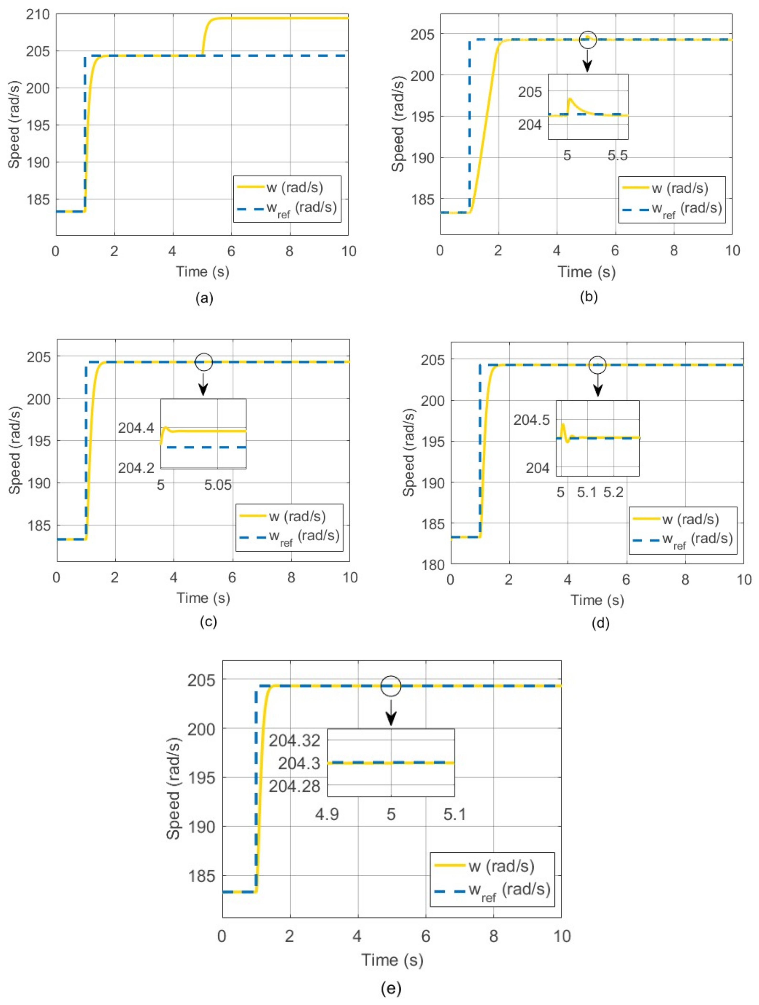
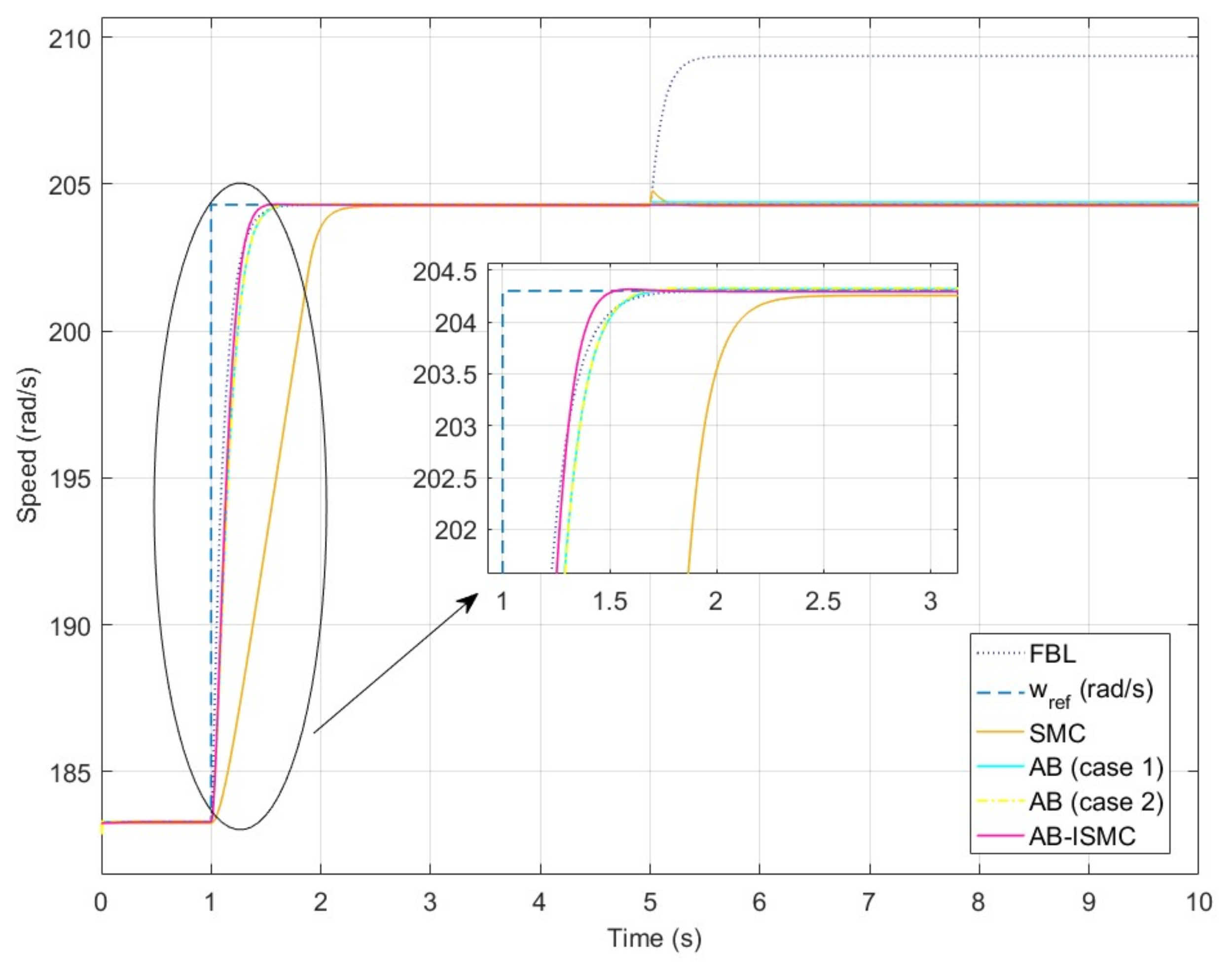
4. Simulation Results

For the simulations and analysis of this study, we utilized an HP ProBook laptop equipped with an Intel Core i5, 10th GEN processor and 8.00 GB RAM. The computing device operates on Windows 11 Pro and MATLAB R2016a/Simulink software is utilized for simulations and data analysis. This section compares the performance of controllers in the weak field region using the minimization criteria: integral square error (ISE), integral absolute error (IAE), and integral time absolute error (ITAE). These criteria are statistical parameters that evaluate the system’s design performance. Furthermore, we analyze the results in more detail using graphical analysis.
The results in Figure 2 demonstrate the impact of parametric uncertainties present in R a , R f and disturbance in load on the system’s performance. At the start, the motor is set to track a reference speed of 183.26 rad/s. Then, at t = 5 s, a disturbance is introduced in one of the following parameters: R a , R f , or the load torque. Specifically, a sudden change of 9 Nm in load torque is introduced at 5 s. The regression criteria (ITAE, IAE, and ISE) are calculated and presented in Table 2. Furthermore, Figure 2 compares the actual speeds of all implemented nonlinear control techniques with the desired speed.
The FBL demonstrates high regression parameter values ( 189.5 , 27.15 , 151.1 rad/s) and exhibits a lack of robustness, as indicated by the steady-state error of 5 rad/s in rotor speed after the introduction of the load disturbance at t = 5 s (refer to Figure 2a). This suggests that the FBL does not effectively reject disturbances and does not attain robust performance. The SMC also exhibited high regression parameter values (i.e., ITAE: 17.54 rad/s, IAE: 11.81 rad/s, and ISE: 170.1 rad/s). However, Figure 2b shows that the SMC effectively rejects the load torque disturbance and returns to the reference speed after a slight peak. As a result, the SMC demonstrates characteristics of robust performance. Compared to the FBL and SMC, the regression parameter values for AB (case 1 and case 2) are lower for all three parameters (i.e., ITAE: 7.072 , 5.153 rad/s, IAE: 3.902 , 3.675 rad/s and ISE: 45.47 , 45.63 rad/s). However, upon observing the results in Figure 2c, one can see that AB (case 1) cannot reject the disturbance, resulting in a steady-state error of 0.1 rad/s after the introduction of the load disturbance at t = 5 s. Therefore, AB (case 1) does not demonstrate robust performance. In contrast, Figure 2d shows that AB (case 2) successfully rejected the load torque disturbance and returned to the reference speed after a slight peak. The values of evaluating parameters for AB–ISMC are considerably lower, as shown in Table 2. It can be seen in Figure 2e that this controller rejected the parametric uncertainties and returns to the reference speed. Hence, this designed controller shows robustness in the presence of variations introduced during the SEDCM operation.
Figure 3 illustrates the system’s speed monitoring and provides visual information about the respective settling time for each of the designed controllers. Initially, the motor is set to operate at a speed of 183.26 rad/s. However, at t = 1 s, the speed is increased to 204.3 rad/s.
The FBL technique demonstrates a favorable settling time of 0.656 s compared to SMC, but suffers from a significant steady-state error of 5 rad/s when subjected to load disturbances. On the other hand, SMC has the highest settling time of 1.481 s, but it effectively rejects the load torque disturbance and returns to the reference speed after a slight peak. The AB controllers (case 1 and case 2) exhibit comparatively lower settling time than FBL and SMC ( 0.619 s and 0.607 s, respectively). However, after the load torque disturbance is applied in case 1, a steady-state error of 0.1 rad/s is observed. Compared to all of the above control techniques, the proposed controller (AB–ISMC) has a minimum settling time of 0.477 s. This depicts good speed tracking characteristics and improves settling time by factors of 27 % , 67 % , 23 % , and 21 % compared to FBL, SMC, and AB controllers (case 1 and case 2), respectively, demonstrating its superior performance characteristics.
AB–ISMC is a novel technique and has numerous distinguishing factors. However, there are a few challenges associated with AB–ISMC. AB–ISMC is able to reduce the chattering effect, which is an inherent problem in SMC-based techniques. But it is still not a chattering-free strategy. AB–ISMC requires careful tuning, especially for complex and high-dimensional systems. Moreover, AB–ISMC is an intricate control strategy that demands a good understanding of the system dynamics and mathematical modeling.

5. Conclusions and Future Work

This study aimed to evaluate and compare the performance of different control methods for the SEDCM in the weak field region, specifically focusing on their ability to reject load disturbances in speed control applications. The simulations were conducted using MATLAB/Simulink. The synergy of adaptive backstepping and integral sliding mode control (AB–ISMC) produced the best results, with the lowest statistical parameter values and the minimum settling time in comparison with other implemented methods. Future research could involve the hardware implementation of the designed controllers with an actual SEDCM. These results could then be compared to the simulation study to gain additional insight into the topic. Moreover, considering discrete implementations of controllers can improve their effectiveness in practical applications. Additionally, expanding the scope of the study to investigate intelligent control techniques such as fuzzy logic and neural networks can contribute toward further development in the topic under consideration.
The focus of the present work is to design and simulate model-based nonlinear control strategies for a SEDCM. Simulation results evidenced the feasibility and overperformance of the proposed strategies in comparison with other controllers. In the near future, we intend to realize the proposed control law on a multi-degree-of-freedom robotic manipulator actuated with SEDCM. Such a manipulator is a highly nonlinear system having coupled dynamics and is thus anticipated to present several interesting challenges in the realization of AB–ISMC law.

Author Contributions

Conceptualization, M.P.; methodology, R.A.; software, R.A.; validation, S.A. and J.I.; formal analysis, R.A.; investigation, R.A.; resources, J.I.; data curation, R.A. and S.A.; writing—original draft preparation, R.A.; writing—review and editing, S.A., J.I. and M.P.; visualization, R.A. and S.A.; supervision, J.I. and M.P.; project administration, J.I. All authors have read and agreed to the published version of the manuscript.

Funding

This research received no external funding.

Institutional Review Board Statement

Not applicable.

Informed Consent Statement

Not applicable.

Data Availability Statement

Not applicable.

Conflicts of Interest

The authors declare no conflict of interest.

Abbreviations

The following abbreviations are used in this manuscript:
ABadaptive backstepping
ABCartificial bee colony
AB–ISMCadaptive backstepping integral sliding mode controller
BSCbackstepping controller
FBLfeedback linearization
FLCfuzzy logic controller
FOSMCfractional-order SMC
IAEintegral absolute error
IMinduction motor
IOFLinput–output feedback linearization
ISEintegral square error
ISMCintegral sliding mode control
ITAEintegral time absolute error
MIMOmulti-input-and-multi-output
PDproportional–derivative
PIproportional–integral
PIDproportional–integral–derivative
PMSMspermanent magnet synchronous motors
SEDCMseparately excited DC motor

References

  1. Riaz, S.; Qi, R.; Tutsoy, O.; Iqbal, J. A novel adaptive PD-type iterative learning control of the PMSM servo system. PLoS ONE 2023, 18, e0279253. [Google Scholar] [CrossRef] [PubMed]
  2. Saleem, O.; Ali, S.; Iqbal, J. Robust MPPT control of stand-alone photovoltaic systems via adaptive fractional-order PID controller with self-adjusting fractional orders. Energies 2023, 16, 5039. [Google Scholar] [CrossRef]
  3. Harrouz, A.; Becheri, H.; Colak, I.; Kayisli, K. Backstepping control of a separately excited DC motor. Electr. Eng. 2018, 100, 1393–1403. [Google Scholar] [CrossRef]
  4. Singh, N.; Sharma, A.K.; Tiwari, M.; Jasiński, M.; Leonowicz, Z.; Rusek, S.; Gono, R. Robust Control of SEDCM by Fuzzy-PSO. Electronics 2023, 12, 335. [Google Scholar] [CrossRef]
  5. Balding, S.; Gning, A.; Cheng, Y.; Iqbal, J. Information rich voxel grid for use in heterogeneous multi-agent robotics. Appl. Sci. 2023, 13, 5065. [Google Scholar] [CrossRef]
  6. Tajudin, A.I.; Izani, M.A.D.; Samat, A.A.A.; Omar, S.; Idin, M.A.M. Design a speed control for DC motor using an optimal PID controller implementation of ABC algorithm. In Proceedings of the IEEE 12th International Conference on Control System, Computing and Engineering (ICCSCE), Penang, Malaysia, 21–22 October 2022; pp. 97–102. [Google Scholar]
  7. Ahmed, A.; Javed, S.B.; Uppal, A.A.; Iqbal, J. The Development of CAVLAB—A control-oriented MATLAB based simulator for an underground coal gasification process. Mathematics 2023, 11, 2493. [Google Scholar] [CrossRef]
  8. Gangwar, A.D.; Sharma, A.; Singh, T.V.P.; Gao, S. Fuzzy logic and PI based closed-loop speed control of a separately excited DC motor using DC-DC converter. In Proceedings of the 2022 2nd Asian Conference on Innovation in Technology (ASIANCON), Ravet, India, 26–28 August 2022; pp. 1–6. [Google Scholar]
  9. Koondhar, M.; Channa, I.; Bukhari, S.; Jamali, M. PI and fuzzy logic controller based comparative analysis of separately excited DC motor. J. Appl. Emerg. Sci. 2021, 11, 52. [Google Scholar]
  10. Soumana, R.A.; Saulo, M.J.; Muriithi, C.M. Enhanced speed control of separately excited DC motor using fuzzy-neural networks controller. In Proceedings of the 2022 4th International Conference on Smart Systems and Inventive Technology (ICSSIT), Tirunelveli, India, 20–22 January 2022; pp. 729–736. [Google Scholar]
  11. Sagar, J.D. DC Motor Control using PID Controller. Int. Res. J. Eng. Technol. 2020, 7, 1765–1769. [Google Scholar]
  12. Wati, T.; Subiyanto; Sutarno. Simulation model of speed control DC motor using fractional order PID controller. J. Phys. Conf. Ser. 2020, 1444, 012022. [Google Scholar] [CrossRef]
  13. Saleem, O.; Abbas, F.; Iqbal, J. Complex fractional-order LQIR for inverted-pendulum-type robotic mechanisms - Design and experimental validation. Mathematics 2023, 11, 913. [Google Scholar] [CrossRef]
  14. Vesović, M.; Jovanović, R.; Trišović, N. Control of a DC motor using feedback linearization and gray wolf optimization algorithm. Adv. Mech. Eng. 2022, 14, 16878132221085324. [Google Scholar] [CrossRef]
  15. Labbadi, M.; Iqbal, J.; Djemai, M.; Boukal, Y.; Bouteraa, Y. Robust tracking control for a quadrotor subjected to disturbances using new hyperplane-based fast terminal sliding mode. PLoS ONE 2023, 18, e0283195. [Google Scholar] [CrossRef] [PubMed]
  16. Ahmad, S.; Uppal, A.A.; Azam, M.R.; Iqbal, J. Chattering free sliding mode control and state dependent kalman filter design for underground coal gasification energy conversion process. Electronics 2023, 12, 876. [Google Scholar] [CrossRef]
  17. Sarker, S.K.; Das, S.K. High performance nonlinear controller design for AC and DC machines: Partial feedback linearization approach. Int. J. Dyn. Control 2018, 6, 679–693. [Google Scholar] [CrossRef]
  18. Gou, L.; Wang, C.; Zhou, M.; You, X. Integral sliding mode control for starting speed sensorless controlled induction motor in the rotating condition. IEEE Trans. Power Electron. 2020, 35, 4105–4116. [Google Scholar] [CrossRef]
  19. Zaihidee, M.F.; Mekhilef, S.; Mubin, M. Robust speed control of PMSM using sliding mode control (SMC)—A review. Energies 2019, 12, 1669. [Google Scholar] [CrossRef] [Green Version]
  20. Ali, S.; Prado, A.; Pervaiz, M. Hybrid backstepping-super twisting algorithm for robust speed control of a three-phase induction motor. Electronics 2023, 12, 681. [Google Scholar] [CrossRef]
  21. Wang, Y.; Yu, H.T.; Feng, N.J.; Wang, Y.C. Non-cascade backstepping sliding mode control with three-order extended observer for PMSM drive. IET Power Electron. 2020, 13, 307–316. [Google Scholar] [CrossRef]
  22. Al-Samarraie, S.A.; Gorial, I.I.; Mshari, M.H. An integral sliding mode control for the magnetic levitation system based on backstepping approach. Iop Conf. Ser. Mater. Sci. Eng. 2020, 881, 012136. [Google Scholar] [CrossRef]
  23. Ali, N.; Alam, W.; Pervaiz, M.; Iqbal, J. Nonlinear adaptive backstepping control of permanent magnet synchronous motor. Revue Roumaine Des Sciences Techniques—Série Électrotechnique et Énergétique 2021, 66, 9–14. [Google Scholar]
  24. Khalil, H.K. Nonlinear Control; Pearson: New York, NY, USA, 2015. [Google Scholar]
  25. Nettari, Y.; Labbadi, M.; Kurt, S. Adaptive backstepping integral sliding mode control combined with super twisting algorithm for nonlinear UAV quadrotor system. IFAC Pap. Online 2022, 55, 264–269. [Google Scholar] [CrossRef]
  26. Zhang, S.; Wang, Q.; Yang, G.; Zhang, M. Anti-disturbance backstepping control for air-breathing hypersonic vehicles based on extended state observer. ISA Trans. 2019, 92, 84–93. [Google Scholar] [CrossRef] [PubMed]
  27. Glushchenko, A.I.; Petrov, V.A.; Lastochkin, K.A. Method development of speed control of DC drive on basis of its feedback linearization. In Proceedings of the European Control Conference (ECC), St. Petersburg, Russia, 12–15 May 2020; pp. 1567–1572. [Google Scholar]
  28. Anjum, M.; Khan, Q.; Ullah, S.; Hafeez, G.; Fida, A.; Iqbal, J.; Albogamy, F.R. Maximum power extraction from a standalone photo voltaic system via neuro-adaptive arbitrary order sliding mode control strategy with high gain differentiation. Appl. Sci. 2022, 12, 2773. [Google Scholar] [CrossRef]
  29. Chand, A.; Khan, Q.; Alam, W.; Khan, L.; Iqbal, J. Certainty equivalence-based robust sliding mode control strategy and its application to uncertain PMSG-WECS. PLoS ONE 2023, 18, e0281116. [Google Scholar] [CrossRef] [PubMed]
  30. Ali, K.; Mehmood, A.; Iqbal, J. Fault-tolerant scheme for robotic manipulator—Nonlinear robust back-stepping control with friction compensation. PLoS ONE 2021, 16, e0256491. [Google Scholar] [CrossRef]
  31. Awan, Z.; Ali, K.; Iqbal, J.; Mehmood, A. Adaptive backstepping based sensor and actuator fault tolerant control of a manipulator. J. Electr. Eng. Technol. 2019, 14, 2497–2504. [Google Scholar] [CrossRef]
  32. Ardhenta, L.; Subroto, R.K.; Hasanah, R.N. Adaptive backstepping control for Buck DC/DC converter and DC motor. J. Phys. Conf. Ser. 2020, 1595, 012025. [Google Scholar] [CrossRef]
  33. Slotine, J.J.E.; Li, W. Applied Nonlinear Control; Prentice Hall: Englewood Cliffs, NJ, USA, 1991; p. 705. [Google Scholar]
  34. Fradkov, A.L.; Miroshnik, I.V.; Nikiforov, V.O. Nonlinear and Adaptive Control of Complex Systems; Springer Science & Business Media: New York, NY, USA, 2013. [Google Scholar]
Figure 1. Separately excited DC motor.
Robotics 12 00105 g001
Figure 2. Output speed signals: (a) FBL, (b) SMC, (c) AB (case 1), (d) AB (case 2), (e) AB–ISMC.
Robotics 12 00105 g002
Figure 3. Comparative results of various control strategies illustrating the output speed of motors.
Robotics 12 00105 g003
Table 1. Parameters of SEDCM.
ParameterSymbolNumerical ValueUnit
Rated PowerP 3.73 kW
Rated Speed w N 183.26 rad/s
Armature Resistance R a 1.2 Ω
Field Resistance R f 60 Ω
Armature Inductance L a 0.01 H
Field Inductance L f 60H
Motor ConstantK 0.3 Nm/A 2
Damping ConstantB 0.011 kgm 2 s 1
InertiaJ 0.208 kgm 2
Armature Voltage u a 240V
Field Voltage u f 240V
Rated Torque τ 18Nm
Table 2. Numerical evaluation.
Control TechniqueITAE (rad/s)IAE (rad/s)ISE (rad/s)
FBL 189.5 27.15 151.1
SMC 17.54 11.81 170.1
AB (case 1) 7.072 3.902 45.47
AB (case 2) 5.153 3.675 45.63
AB–ISMC 3.569 3.086 41.36
Disclaimer/Publisher’s Note: The statements, opinions and data contained in all publications are solely those of the individual author(s) and contributor(s) and not of MDPI and/or the editor(s). MDPI and/or the editor(s) disclaim responsibility for any injury to people or property resulting from any ideas, methods, instructions or products referred to in the content.

