Inverse Kinematics of an Anthropomorphic 6R Robot Manipulator Based on a Simple Geometric Approach for Embedded Systems

Abstract

This manuscript presents an efficient algorithm for solving the inverse kinematics problem of a 6R robot manipulator to be deployed on embedded control hardware. The proposed method utilizes the geometric relationship between the end-effector and the base of the manipulator, resulting in a computationally efficient solution. The approach aims to minimize computational complexity and memory consumption while maintaining the accuracy and real-time performance demonstrated by simulations and verified by experimental results on an embedded system. Furthermore, the manipulator is analyzed in terms of singularities, limits, the workspace, and general solvability. Due to the simplicity of the algorithm, a platform-independent implementation is possible. As a result, the average calculation time is reduced by a factor of five to eight and the average error is decreased by a factor of fifty compared to a powerful analytical solver.

1. Introduction

The capability to perform fine and intricate movements with its end-effector is essential for mobile manipulators, as it enables the robot to interact with its environment in a more effective and precise manner. A modular adaptable search and rescue robot [1] with dexterous manipulation capabilities can perform a variety of tasks, such as picking up objects, opening doors, and manipulating objects in tight spaces, see Figure 1. The development of such complex systems requires the integration of several different technologies, including robot kinematics, control, sensing, and actuation. The robot’s end-effector is designed to have a high degree of dexterity, with the ability to move in many different directions and orientations. An intuitive Human–Robot Interaction (HRI) approach that allows operators to precisely and accurately control end-effector movements is essential [2].

One approach to achieve dexterous manipulation is to use robotic arms or hands with multiple degrees of freedom (DOF). These types of manipulators can perform a wide range of movements, allowing the robot to interact with its environment in a more flexible manner. The kinematics of the manipulator must be carefully designed to ensure that it has the necessary range of motion and precision for the task at hand. For this purpose, manipulators with six DOF are typically used, e.g., a manipulator consisting of serial links and an end-effector connected with six revolute joints (6R). This is due, among other reasons, to the fact that a minimum of six DOF are required to reach any pose of the tool center point (TCP) within the workspace, which provides a high degree of usability and flexibility. Due to the high nonlinearity of the system, resource-intensive computational algorithms are typically executed on powerful computers to control six DOF manipulators.

For mobile robot platforms, the challenge is that either the data have to be transmitted to the robot or the control unit has to be moved to the platform. For smooth and accurate motions, a large amount of data is generated. Consequently, real-time capable transmission systems with high data transfer rates and a stable transmission link are needed. Since this condition generally cannot be guaranteed in rescue robotics, it is reasonable to perform the calculation directly on the mobile platform. In the case of lightweight rescue robots with a compact design (cf. Figure 1), it is impractical or impossible to move large and heavy computers to the platform, therefore small and lightweight embedded systems are used. However, due to the limited computing power, developing an efficient algorithm that consumes as few computing resources as possible is necessary. Further difficulties arise from the fact that the communication with the robot may be interrupted at any time. In this case, the stable behavior of the manipulator needs to be ensured. As a consequence, differential kinematic approaches to end-effector control are generally excluded, since a stop of the manipulator cannot be ensured.

For the reasons stated, an efficient inverse kinematics (IK) solver to control a custom-built manipulator attached to a mobile robot platform is presented. Based on the requirements for the solver and the geometry of the manipulator, a geometric approach for solving the IK problem is chosen. The developed algorithm is supported by experimental results, which were investigated for the accuracy and real-time capability of the solver on embedded hardware and compared to a powerful analytical kinematics solver. The modularization of the control unit in combination with the manipulator allows the manipulator to be addressed via a predefined interface. As a result, the manipulator can be controlled independently of higher-level control systems.

The presented manuscript contains the following key contributions:

• The fundamental derivation of the forward and inverse kinematics of a 6R robot manipulator, as well as the development of the IK solver in order to resolve the joint angles based on arbitrary TCP poses. The geometric approach is an extension of the inverse kinematic solutions based on industrial robots with respect to the deployment of embedded hardware.
• The analysis of important characteristics, which are essential for the practical application of the solver.
• Simulation results that validate the presented solution to the IK problem and the solver accuracy with high computational power.
• Experimental results that examine the solver accuracy and real-time capability on an embedded open-source 32-bit ARM Cortex^®-M7 board with an FPU and a clock frequency of 260 MHz (https://emanual.robotis.com/docs/en/parts/controller/opencr10/ accessed on 6 July 2023).

When implementing IK on an embedded platform, there are several innovations and considerations that can improve its performance and efficiency. Compared to related work, there are some notable innovations here:

• Efficient IK Solvers: Developing lightweight and efficient IK solvers is crucial for embedded platforms with limited computational resources.
• Real-Time Optimization: Embedded platforms often require real-time performance for controlling robots in dynamic environments. The developed algorithm can efficiently handle constraints and optimize IK solutions within the given time constraints.
• Memory Optimization: Embedded platforms often have limited memory resources. Optimizing data structures, algorithms, and parameter representations can help reduce memory usage.
• Energy Efficiency: Embedded systems typically operate on limited power sources. Designing energy-efficient IK algorithms by minimizing unnecessary computations, optimizing data flow, or leveraging low-power modes when idle can help prolong the system’s battery life for mobile manipulators.
• Platform-Independent: The platform-independent IK solver presented in this paper offers a versatile and adaptable solution for solving the inverse kinematics problem of robotic manipulators. Decoupling the solver from platform-specific considerations provides a unified framework that can be easily integrated into diverse robotic systems, regardless of the underlying computing platform.

It is important to note that the specific innovations for an IK implementation on an embedded platform may vary depending on the system’s requirements, constraints, and available hardware resources.

2. Related Work

Due to the fact that IK of robots is of central importance in robotics, it has been extensively covered. Fundamental studies of robot manipulators are described by Pieper [3]. Furthermore, it is shown that the IK problem for manipulators with six DOF and spherical wrists can be separated and thus solved geometrically. Lee and Ziegler [4] describe a geometric approach to obtain a closed-form solution for the IK of a robot with a geometric configuration equivalent to that of the PUMA robot. The IK problem is solved in two stages. First, the solution of the first three joints is derived geometrically. Second, the solution of the last three joints is calculated based on the solution of the first three joints to result in the desired orientation of the TCP. The selection of the most suitable solution among several possible solutions is realized via indicators. Lloyd and Hayward [5] provide forward kinematics, analytical IK, and Jacobian solutions of common serial manipulators.

Raghavan and Roth [6] present a solution of the IK problem for robots with general geometry. Through extensive mathematical transformations and simplifications, a univariate 16th order polynomial can be formulated, whose roots can be solved. Subsequently, all remaining unknowns can be solved. The description of the robot kinematics is compatible with the notation according to Denavit and Hartenberg [7], which is commonly used to relate coordinate systems in robotics. Manocha and Canny [8] develop an efficient algorithm to solve the system of equations stated in [6] using eigendecomposition. As a consequence, the calculation time can be significantly reduced.

IK solutions for sixteen different types of manipulators with spherical wrists are provided by Kucuk and Bingul [9]. Thus, closed-form solutions exist for all common manipulators where the last three axes intersect at one common point.

Husty et al. [10] describe an algorithm with a new approach to solving the IK problem compared to previous publications. The geometric structure of the manipulator is considered in the analysis using the study model of Euclidean displacements. Further, techniques of multidimensional geometry are applied to solve the problem. As a result, all sixteen solutions to the IK problem of serial 6R robots with general geometry can be calculated analytically and more efficiently than in [6].

An alternative and more generic description of robot geometry compared to the Denavit–Hartenberg notation [7] is described by Brandstötter et al. [11]. A corresponding forward and closed-form IK solution is stated. As a result, serial 6R robots with ortho-parallel basis and spherical wrists can be defined by seven characteristic parameters, which improves the practicability and applicability of common robots.

Khatamian [12] provides a forward and geometric IK solution to robots with an ortho-parallel basis and a spherical wrist, based on the industrial robot KUKA KR60. An alternative solution to [12], based on the industrial robot COMAU NM45, is proposed by Asif and Webb [13]. Solutions to similar approaches are presented in [14,15,16]. Krishnan and Ashok [17] describe a forward and closed-form analytical IK solution to robots with an ortho-parallel basis and a spherical wrist, based on the industrial robot ABB IRB 1200. Recent publications concentrate on solving the IK problem based on screw theory, e.g., [18,19,20]. In summary, a variety of solutions exist for calculating the IK of 6-DOF robotic manipulators, among other reasons due to their importance in the industry.

The open source framework MoveIt [21], which is integrated into ROS [22], is a widely used software for manipulation. MoveIt provides core functionalities such as motion planning, 3D perception, navigation, and control. Despite the advantages mentioned, MoveIt cannot be executed on embedded systems. The kinematics solver IKFast (http://openrave.org/docs/latest_stable/openravepy/ikfast/ accessed on 6 July 2023) [23] can be used as a plugin for MoveIt, and the source code of the closed-form analytical solution can be exported for independent use. This enables the development of the IK solver in MoveIt and a platform-independent application of the algorithm. Since the source code generated by IKFast has to be extensively adapted to be used on embedded systems and the geometry of the manipulator is not considered in the analytical solution (and thus is more extensive), a geometric IK solver with an approach similar to that proposed in the publications [12,13,15,16] is presented.

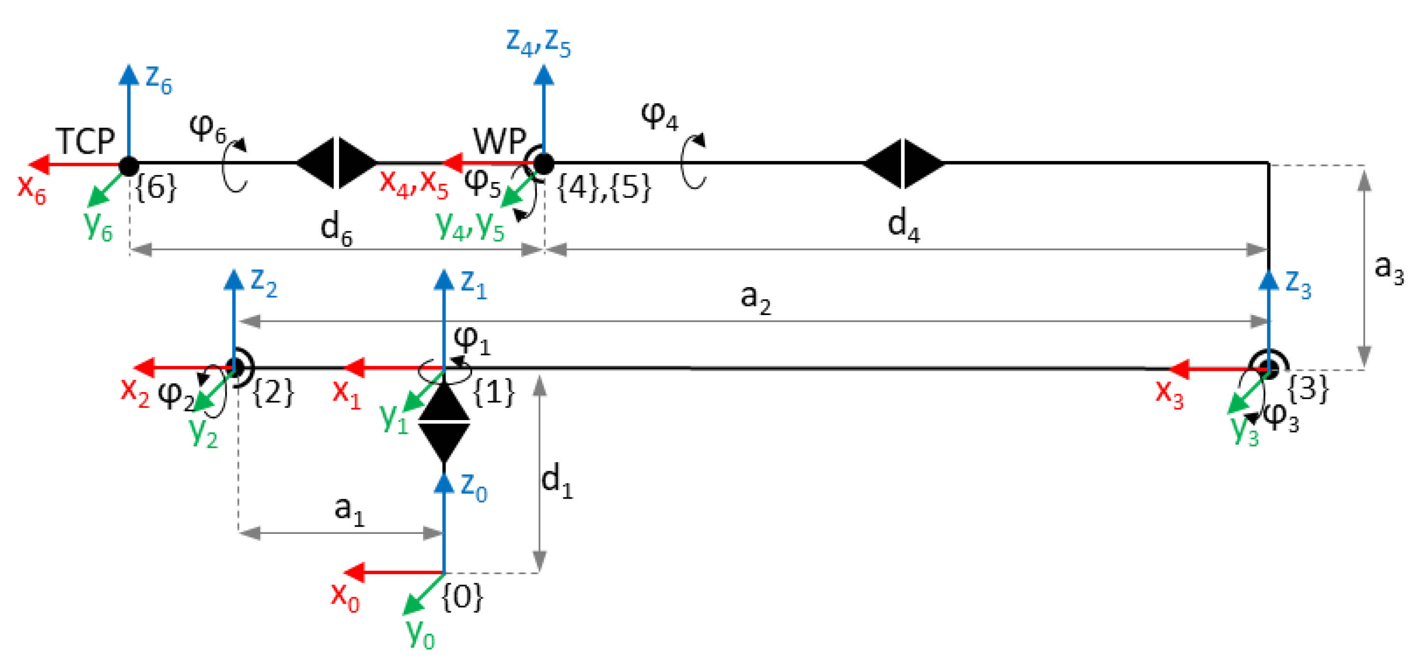
3. Fundamental Geometry

Robot kinematics is based on the geometry of the manipulator and specifies the procedure of the solver development. For this reason, the geometry is analyzed in advance. The kinematic relationships are described by homogeneous transformation matrices (cf. Equation (1)). The homogeneous transformation matrix ${}^i{\mathit{T}}_j$ consists of the translational vector ${}^i{\overrightarrow{p}}_{ij}$ and the rotational matrix ${}^i{\mathit{R}}_j$ (cf. Equations (2) and (3), respectively).

$${}^i{\mathit{T}}_j=\left[\begin{array}{cccc}& & & \\ & {}^i{\mathit{R}}_j& & {}^i{\overrightarrow{p}}_{ij}\\ & & & \\ & {\overrightarrow{0}}^T& & 1\end{array}\right]$$

(1)

$${}^i{\overrightarrow{p}}_{ij}=\left[\begin{array}{c}{}^i{p}_{ij,x}\\ {}^i{p}_{ij,y}\\ {}^i{p}_{ij,z}\end{array}\right]$$

(2)

$${}^i{\mathit{R}}_j=\left[\begin{array}{ccc}{}^i{\overrightarrow{m}}_j& {}^i{\overrightarrow{n}}_j& {}^i{\overrightarrow{o}}_j\end{array}\right]=\left[\begin{array}{ccc}{}^i{m}_{j,x}& {}^i{n}_{j,x}& {}^i{o}_{j,x}\\ {}^i{m}_{j,y}& {}^i{n}_{j,y}& {}^i{o}_{j,y}\\ {}^i{m}_{j,z}& {}^i{n}_{j,z}& {}^i{o}_{j,z}\end{array}\right]$$

(3)

The following notation commonly used in robotics is introduced:

$$\begin{array}{cccc}\hfill C_i& \hfill =cos{\phi }_i\hfill & \hfill C_{ij}& \hfill =cos({\phi }_i-{\phi }_j)\hfill \\ \hfill S_i& \hfill =sin{\phi }_i\hfill & \hfill S_{ij}& \hfill =sin({\phi }_i-{\phi }_j)\hfill \end{array}$$

(4)

A common method to describe the manipulator geometry is the parameterization according to Denavit and Hartenberg [7]. The kinematics of the manipulator can be completely described by the Denavit–Hartenberg parameters $a_i,{\alpha }_i,d_i,\mathrm{and}{\theta }_i$ of each link i and the corresponding coordinate systems, illustrated in

Table 1. Denavit–Hartenberg parameters of the first six DOF from the base to the TCP of the gripper.

Link	Joint Variable	${\mathit{\theta }}_{\mathit{i}}$ [$\mathbf{rad}$]	${\mathit{d}}_{\mathit{i}}$ [$\mathbf{m}$]	${\mathit{a}}_{\mathit{i}}$ [$\mathbf{m}$]	${\mathit{\alpha }}_{\mathit{i}}$ [$\mathbf{rad}$]	Range
1	${\phi }_1$	${\phi }_1$	0.081	0.077	$-\frac{\pi }{2}$	±90${}^{\circ }$
2	${\phi }_2$	${\phi }_2-\pi$	0	0.520	$\pi$	0${}^{\circ }$– 180 ${}^{\circ }$
3	${\phi }_3$	${\phi }_3-\frac{\pi }{2}$	0	0.066	$\frac{\pi }{2}$	0${}^{\circ }$– 180 ${}^{\circ }$
4	${\phi }_4$	${\phi }_4$	0.409	0	$-\frac{\pi }{2}$	±180${}^{\circ }$
5	${\phi }_5$	${\phi }_5$	0	0	$\frac{\pi }{2}$	±90${}^{\circ }$
6	${\phi }_6$	${\phi }_6$	0.180	0	0	$\pm \infty$

and in the schematic sketch in Figure 2. The corresponding CAD drawing of the initial pose of the manipulator is depicted in Figure 3. The joint angles ${\phi }_1\dots {\phi }_5$ are limited by the mechanical structure of the manipulator, and the joint $\left\{6\right\}$ is designed as a continuous joint, thus allowing infinite rotation. The transformation matrix ${}^{i-1}{\mathit{A}}_i$ is used to represent the coordinate system $\left\{i\right\}$ in the coordinate system $\{i-1\}$ based on Denavit–Hartenberg parameters and allows the complete description of the kinematic chain of a rigid body system. The Denavit–Hartenberg transformation matrix is given in Equation (5).

$$\begin{array}{c}\hfill {}^{i-1}{\mathit{A}}_i=Rot(z_{i-1},{\theta }_i)·Trans(z_{i-1},d_i)·Trans(x_i,a_i)·Rot(x_i,{\alpha }_i)=\hfill \\ \hfill \left[\begin{array}{cccc}cos{\theta }_i& -sin{\theta }_i·cos{\alpha }_i& sin{\theta }_i·sin{\alpha }_i& a_i·cos{\theta }_i\\ sin{\theta }_i& cos{\theta }_i·cos{\alpha }_i& -cos{\theta }_i·sin{\alpha }_i& a_i·sin{\theta }_i\\ 0& sin{\alpha }_i& cos{\alpha }_i& d_i\\ 0& 0& 0& 1\end{array}\right]\end{array}$$

(5)

In the context of the 6R manipulator, each revolute joint of the robotic arm is actuated by a Dynamixel Pro (https://emanual.robotis.com/docs/en/dxl/pro/ accessed on 6 July 2023) motor. These motors provide precise control over the joints, enabling accurate positioning and movement of the arm. For communication, the RS485 interface is used, which allows seamless integration of the arm with the embedded board.

Table 2. Motor configurations of the 6-DOF manipulator.

Joint	Motor	Motor Resolution [pulse/rev]
1	H54-100-S500-R	501,923
2	H54-200-S500-R	501,923
3	H54-200-S500-R	501,923
4	H54-100-S500-R	501,923
5	H42-20-S300-R	303,751
6	H42-20-S300-R	303,751

shows the motor configuration. Each joint is connected by rigid links made of lightweight and durable materials such as aluminum or carbon fiber, ensuring strength and flexibility.

Figure 4 illustrates the workspace of a 6R manipulator, which refers to the region in 3D space where the end-effector (the tool or gripper attached to the robot) can reach and operate. The left view orientation shows the vertical and horizontal range of the workspace, which depends on the height of the arm and the orientation of the joints. The arm can reach 3D poses within a sphere with a radius of 1090 mm from the center of joint $\left\{1\right\}$ of the manipulator. The working area from the top view of the manipulator is shown as a two-dimensional projection of the plane. The shape of the working area is influenced by the lengths of the arm segments, the range of the joints, and all physical constraints that limit the movement of the arm with a radius of 1090 mm.

4. Forward Kinematics

Forward kinematics is the determination of the position and orientation of the TCP in relation to the base depending on the joint variables. The forward transformation of serial robots, also referred to as direct transformation, results from a chain transformation of the individual transformation matrices stated in Equation (6) and provides a unique solution for serial robots. The pose of the TCP can thus be expressed by the transformation matrix ${}^0{\mathit{T}}_6$.

$${}^0{\mathit{T}}_6={}^0{\mathit{T}}_1·{}^1{\mathit{T}}_2·{}^2{\mathit{T}}_3·{}^3{\mathit{T}}_4·{}^4{\mathit{T}}_5·{}^5{\mathit{T}}_6$$

(6)

Hence, the calculation of the individual transformation matrices of each link based on the joint variables and manipulator geometry is required. The transformation matrices can be obtained according to the Denavit–Hartenberg convention (cf. Equation (5)). It should be noted that the assignment of the coordinate systems according to the Denavit–Hartenberg convention does not necessarily correspond to the desired assignment of the joint coordinate systems due to the fact that they have to be assigned according to certain criteria in order to comply with the Denavit–Hartenberg convention. Due to this reason, additional transformations may be necessary to achieve the desired representation.

For manipulators with simple geometries, the transformation matrices can alternatively be obtained by translations and elementary rotations in relation to arbitrarily assigned joint coordinate systems. For this robot arm, the forward and inverse kinematics are developed according to the sketch illustrated in Figure 5. The procedure is generally the same, however, the description of the transformation matrices is simplified because they consist of only one translation and rotation instead of two.

5. Inverse Kinematics

Inverse kinematics or backward transformation describes the inverse operation of forward kinematics, i.e., the determination of the joint variables at a given pose of the TCP. In contrast to forward kinematics, inverse kinematics generally does not provide a unique solution. Thus, the robot arm is analyzed to develop an inverse solver in order to resolve the joint angles $({\phi }_1\dots {\phi }_6)$ based on the pose of the TCP.

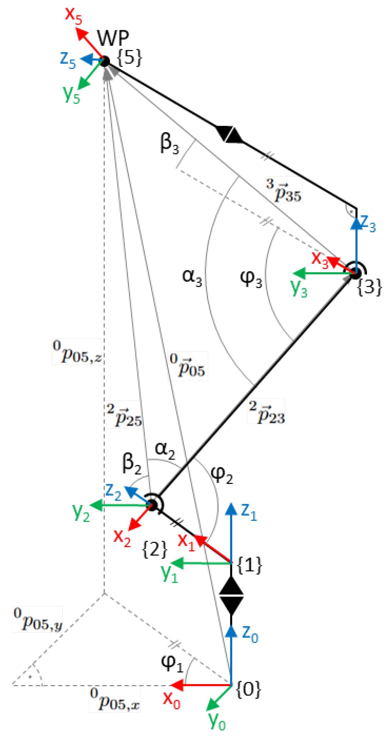
5.1. Geometric Derivation

Given that the axes of joints $\left\{4\right\}$, $\left\{5\right\}$, and $\left\{6\right\}$ intersect at a single point, the IK can be solved geometrically (described by Pieper [3], cf. e.g., [24] (p. 29)). The position of the intersection point of the axes is independent of the joint angles ${\phi }_4\dots {\phi }_6$ and results directly from the given goal pose of the TCP. Consequently, the joint angles ${\phi }_1\dots {\phi }_3$ of joints $\left\{1\right\}$, $\left\{2\right\}$, and $\left\{3\right\}$ can be calculated by geometric considerations based on the known position of the wrist point (WP, intersection point of the axes) illustrated in Figure 6. Due to the given goal orientation ${}^0{\mathit{R}}_6$ of the TCP and the calculated angles ${\phi }_1\dots {\phi }_3$, the angles ${\phi }_4\dots {\phi }_6$ can then be resolved analytically. Mathematically, this means a separation of the problem in two sub-problems. The basic procedure is described by the following Equations (7) and (8):

$${}^0{\overrightarrow{p}}_{05}={}^0{\overrightarrow{p}}_{04}={}^0{\overrightarrow{p}}_{02}\left({\phi }_1\right)+{}^0{\overrightarrow{p}}_{25}({\phi }_2,{\phi }_3)$$

(7)

$$\begin{array}{cc}\hfill {}^3{\mathit{R}}_6({\phi }_1,{\phi }_2,{\phi }_3)& ={}^3{\mathit{R}}_6({\phi }_4,{\phi }_5,{\phi }_6)\hfill \\ \hfill {\left({}^0{\mathit{R}}_1\left({\phi }_1\right)·{}^1{\mathit{R}}_2\left({\phi }_2\right)·{}^2{\mathit{R}}_3\left({\phi }_3\right)\right)}^{-1}·{}^0{\mathit{R}}_6& ={}^3{\mathit{R}}_4\left({\phi }_4\right)·{}^4{\mathit{R}}_5\left({\phi }_5\right)·{}^5{\mathit{R}}_6\left({\phi }_6\right)\hfill \end{array}$$

(8)

Hence, the calculated solutions for the joint angles ${\phi }_1\dots {\phi }_6$ result in the exact position ${}^0{\overrightarrow{p}}_{06}$ and orientation ${}^0{\mathit{R}}_6$ of the TCP (specified by the goal pose ${}^0{\mathit{T}}_6$).

Due to the kinematics of the manipulator, there are eight different solutions of combinations of joint angles to obtain the desired pose of the end-effector. This results because

• the link between the coordinate systems $\left\{1\right\}$ and $\left\{2\right\}$ can be oriented towards or opposite from the WP,
• the elbow defined by the coordinate system $\left\{3\right\}$ can be oriented upwards or downwards, and
• the orientation of the wrist is identical every half turn of the joints assigned to the coordinate systems $\left\{4\right\}$ and $\left\{6\right\}$ and the corresponding angle of the joint assigned to the coordinate system $\left\{5\right\}$,

hence $2^3=8$ solutions. Based on the combinations of joint angles, the joints of the manipulator can be divided into the following three subgroups consisting of

• joint $\left\{1\right\}$ (shoulder);
• joints $\left\{2\right\}$ and $\left\{3\right\}$ (elbow);
• joints $\left\{4\right\}$, $\left\{5\right\}$, and $\left\{6\right\}$ (wrist).

As a result, the IK problem can be further divided into three problems corresponding to each joint subgroup, whose solutions are described in Section 5.2.

5.2. Solution

5.2.1. Joint 1

The given goal pose of the TCP represented by the transformation matrix ${}^0{\mathit{T}}_6$ is defined in Equation (9):

$${}^0{\mathit{T}}_6=\left[\begin{array}{cccc}\overrightarrow{m}& \overrightarrow{n}& \overrightarrow{o}& \overrightarrow{p}\\ 0& 0& 0& 1\end{array}\right]=\left[\begin{array}{cccc}{m}_x& n_x& o_x& p_x\\ m_y& n_y& o_y& p_y\\ m_z& n_z& o_z& p_z\\ 0& 0& 0& 1\end{array}\right]$$

(9)

In this specific case, superscripts and subscripts of the coordinate systems are omitted due to better readability and because of the significance of the matrix ${}^0{\mathit{T}}_6$ and its entries in the further course. Using the goal pose of the TCP ${}^0{\mathit{T}}_6$, the link length $d_6$ and the joint angle ${\phi }_6$, the transformation between base $\left\{0\right\}$, WP$\left\{5\right\}$, and TCP$\left\{6\right\}$ can be described (cf. Equation (10)).

$${}^0{\mathit{T}}_6={}^0{\mathit{T}}_5·{}^5{\mathit{T}}_6={}^0{\mathit{T}}_5·Trans(d_6,0,0)·Rot(x,{\phi }_6)={}^0{\mathit{T}}_5·\left[\begin{array}{cccc}1& & 0& d_6\\ 0& C_6& -S_6& 0\\ 0& S_6& C_6& 0\\ 0& 0& 0& 1\end{array}\right]$$

(10)

Using Equation (10) and the inverse transformation matrix ${{}^5{\mathit{T}}_6}^{-1}$ (cf. Equation (11)),

$${}^6{\mathit{T}}_5={{}^5{\mathit{T}}_6}^{-1}=\left[\begin{array}{cccc}1& & 0& -d_6\\ 0& C_6& S_6& 0\\ 0& -S_6& C_6& 0\\ 0& 0& 0& 1\end{array}\right]$$

(11)

the position ${}^0{\overrightarrow{p}}_{05}$ of the WP with reference to the base coordinate system $\left\{0\right\}$ can be calculated (cf. Equations (12) and (13)).

$${}^0{\mathit{T}}_5={}^0{\mathit{T}}_6·{{}^5{\mathit{T}}_6}^{-1}={}^0{\mathit{T}}_6·{}^6{\mathit{T}}_5=\left[\begin{array}{cccc}& & & p_x-d_6·m_x\\ & {}^0{\mathit{R}}_5& & p_y-d_6·m_y\\ & & & p_z-d_6·m_z\\ 0& 0& 0& 1\end{array}\right]$$

(12)

$${}^0{\overrightarrow{p}}_{05}={}^0{\overrightarrow{p}}_{06}-d_6·\overrightarrow{m}=\left[\begin{array}{c}{p}_x-d_6·m_x\\ p_y-d_6·m_y\\ p_z-d_6·m_z\end{array}\right]$$

(13)

Solution for Joint 1: The plane spanned by the rotation of joint angle ${\phi }_1$ is orthogonal to the plane spanned by the rotation of joint angles ${\phi }_2$ and ${\phi }_3$, because the axis $\left\{1\right\}$ is perpendicular to the axes $\left\{2\right\}$ and $\left\{3\right\}$. Consequently, the joint angle ${\phi }_1$ can be calculated using the x and y components of the vector ${}^0{\overrightarrow{p}}_{05}$ from the base to the WP (cf. Equation (14)).

$${\phi }_1=\left\{\begin{array}{cc}atan2({}^0{p}_{05,y},{}^0{p}_{05,x})\hfill & \mathrm{towards}\mathit{WP}\hfill \\ \hfill atan2(-{}^0{p}_{05,y},-{}^0{p}_{05,x})\hfill & \hfill \mathrm{away}\mathrm{from}\mathit{WP}\hfill \end{array}\right.$$

(14)

5.2.2. Joints 2 and 3

Using the calculated joint angle ${\phi }_1$, the transformation matrix ${}^0{\mathit{T}}_2$ from the base $\left\{0\right\}$ to coordinate system $\left\{2\right\}$ can be calculated via forward transformation (cf. Equations (15)–(17)).

$${}^0{\mathit{T}}_1=Trans(0,0,d_1)·Rot(z,{\phi }_1)=\left[\begin{array}{cccc}{C}_1& -S_1& 0& 0\\ S_1& C_1& 0& 0\\ 0& 0& 1& d_1\\ 0& 0& 0& 1\end{array}\right]$$

(15)

$${}^1{\mathit{T}}_2=Trans(a_1,0,0)·Rot(y,{\phi }_2)=\left[\begin{array}{cccc}{C}_2& 0& S_2& a_1\\ 0& 1& 0& 0\\ -S_2& 0& C_2& 0\\ 0& 0& 0& 1\end{array}\right]$$

(16)

$${}^0{\mathit{T}}_2={}^0{\mathit{T}}_1·{}^1{\mathit{T}}_2=\left[\begin{array}{cccc}& & & a_1·C_1\\ & {}^0{\mathit{R}}_2& & a_1·S_1\\ & & & d_1\\ 0& 0& 0& 1\end{array}\right]$$

(17)

The translation vector ${}^0{\overrightarrow{p}}_{02}$ (cf. Equation (18)) results directly from the transformation matrix ${}^0{\mathit{T}}_2$.

$${}^0{\overrightarrow{p}}_{02}=\left[\begin{array}{c}{a}_1·C_1\\ a_1·S_1\\ d_1\end{array}\right]$$

(18)

From the vectors ${}^0{\overrightarrow{p}}_{02}$ and ${}^0{\overrightarrow{p}}_{05}$ (cf. Equations (18) and (13), respectively), the vector ${}^0{\overrightarrow{p}}_{25}$ can be calculated (cf. Equation (19)), which represents the translation between the coordinate system $\left\{2\right\}$ and the coordinate system $\left\{5\right\}$ of the WP.

$${}^0{\overrightarrow{p}}_{25}={}^0{\overrightarrow{p}}_{05}-{}^0{\overrightarrow{p}}_{02}=\left[\begin{array}{c}{p}_x-d_6·m_x-a_1·C_1\\ p_y-d_6·m_y-a_1·S_1\\ p_z-d_6·m_z-d_1\end{array}\right]$$

(19)

The vectors ${}^2{\overrightarrow{p}}_{23}$ and ${}^3{\overrightarrow{p}}_{35}$ can be set up by geometrical considerations (cf. Equations (20) and (21), respectively).

$${}^2{\overrightarrow{p}}_{23}=\left[\begin{array}{c}-a_2\\ 0\\ 0\end{array}\right]$$

(20)

$${}^3{\overrightarrow{p}}_{35}=\left[\begin{array}{c}{d}_4\\ 0\\ a_3\end{array}\right]$$

(21)

The vectors ${\overrightarrow{p}}_{25}$, ${\overrightarrow{p}}_{23}$, and ${\overrightarrow{p}}_{35}$ form a triangle whose vertices are located at the origins of the coordinate systems $\left\{2\right\}$, $\left\{3\right\}$, and $\left\{5\right\}$ (WP). The square of the vector length is obtained via the vector norm (cf. Equations (22)–(24)). Subsequently, the angles ${\phi }_2$ and ${\phi }_3$ can be calculated using the law of cosines.

$$\begin{array}{c}{||{\overrightarrow{p}}_{25}||}^2={||{}^0{\overrightarrow{p}}_{25}||}^2={{}^0{p}_{25,x}}^2+{{}^0{p}_{25,y}}^2+{{}^0{p}_{25,z}}^2=\hfill \\ \hfill {(p_x-d_6·m_x-a_1·C_1)}^2+{(p_y-d_6·m_y-a_1·S_1)}^2+{(p_z-d_6·m_z-d_1)}^2\end{array}$$

(22)

$${||{\overrightarrow{p}}_{23}||}^2={||{}^2{\overrightarrow{p}}_{23}||}^2={a_2}^2$$

(23)

$${||{\overrightarrow{p}}_{35}||}^2={||{}^3{\overrightarrow{p}}_{35}||}^2={d_4}^2+{a_3}^2$$

(24)

To calculate the elevation angle ${\beta }_2$, the vector ${}^0{\overrightarrow{p}}_{25}$ is transformed into the coordinate system $\left\{1\right\}$ using the inverse of the rotation matrix ${}^0{\mathit{R}}_1$ (cf. Equation (25)).

$${}^1{\overrightarrow{p}}_{25}={{}^0{\mathit{R}}_1}^{-1}·{}^0{\overrightarrow{p}}_{25}={}^1{\mathit{R}}_0·{}^0{\overrightarrow{p}}_{25}$$

(25)

The calculation of the elevation angle ${\beta }_2$ can thus be done via the x and z components of the vector ${}^1{\overrightarrow{p}}_{25}$, with the z component remaining unchanged by the transformation from the base coordinate system $\left\{0\right\}$ to coordinate system $\left\{1\right\}$ (cf. Equations (26) and (27)).

$${}^1{p}_{25,x}=p_x·C_1+p_y·S_1-a_1-d_6·(m_x·C_1+m_y·S_1)$$

(26)

$${}^1{p}_{25,z}={}^0{p}_{25,z}=p_z-d_6·m_z-d_1$$

(27)

Solution for Joint 2: The solution for ${\phi }_2$ can be calculated based on the elevation angle ${\beta }_2$ and the triangular angle ${\alpha }_2$ (cf. Equations (28) and (29), respectively).

$${\beta }_2=atan2({}^1{p}_{25,z},{}^1{p}_{25,x})$$

(28)

$${\alpha }_2=arccos\left(\frac{{||{\overrightarrow{p}}_{23}||}^2+{||{\overrightarrow{p}}_{25}||}^2-{||{\overrightarrow{p}}_{35}||}^2}{2·||{\overrightarrow{p}}_{23}||·||{\overrightarrow{p}}_{25}||}\right)$$

(29)

Due to geometrical considerations, the following two solutions for the joint angle ${\phi }_2$ result (cf. Equation (30)):

$${\phi }_2=\left\{\begin{array}{cc}\pi -{\alpha }_2-{\beta }_2\hfill & \mathrm{elbow}\mathrm{up}\hfill \\ \pi +{\alpha }_2-{\beta }_2\hfill & \mathrm{elbow}\mathrm{down}\hfill \end{array}\right.$$

(30)

Solution for Joint 3: Likewise, the offset angle ${\beta }_3$ and the triangular angle ${\alpha }_3$ can be calculated (cf. Equations (31) and (32), respectively).

$${\beta }_3=arctan\left(\frac{{}^3{p}_{35,z}}{{}^3{p}_{35,x}}\right)=arctan\left(\frac{a_3}{d_4}\right)$$

(31)

$${\alpha }_3=arccos\left(\frac{{||{\overrightarrow{p}}_{23}||}^2+{||{\overrightarrow{p}}_{35}||}^2-{||{\overrightarrow{p}}_{25}||}^2}{2·||{\overrightarrow{p}}_{23}||·||{\overrightarrow{p}}_{35}||}\right)$$

(32)

The angles ${\alpha }_3$ and ${\beta }_3$ result in the joint angle ${\phi }_3$ (cf. Equation (33)):

$${\phi }_3=\left\{\begin{array}{cc}{\alpha }_3-{\beta }_3\hfill & \mathrm{elbow}\mathrm{up}\hfill \\ 2\pi -{\alpha }_3-{\beta }_3\hfill & \mathrm{elbow}\mathrm{down}\hfill \end{array}\right.$$

(33)

5.2.3. Joints 4, 5, and 6

Based on the joint angles ${\phi }_1\dots {\phi }_3$, the rotation matrix ${}^0{\mathit{R}}_3$ can be calculated by forward transformation (cf. Equation (34)).

$${}^0{\mathit{R}}_3={}^0{\mathit{R}}_1·{}^1{\mathit{R}}_2·{}^2{\mathit{R}}_3=Rot(z,{\phi }_1)·Rot(y,{\phi }_2)·Rot(y,-{\phi }_3)$$

(34)

Subsequently, the rotation matrix ${}^3{\mathit{R}}_6$ can be determined using the given orientation matrix of the TCP ${}^0{\mathit{R}}_6$ (cf. Equation (35))

$${}^3{\mathit{R}}_6={{}^0{\mathit{R}}_3}^{-1}·{}^0{\mathit{R}}_6={{}^0{\mathit{R}}_3}^T·{}^0{\mathit{R}}_6={}^3{\mathit{R}}_0·{}^0{\mathit{R}}_6$$

(35)

to obtain the corresponding matrix entries (cf. Equation (36)).

$$\begin{array}{cc}\hfill {}^3{m}_{6,x}& =(m_x·C_1+m_y·S_1)·C_{23}-m_z·S_{23}\hfill \\ \hfill {}^3{m}_{6,y}& =m_y·C_1-m_x·S_1\hfill \\ \hfill {}^3{m}_{6,z}& =(m_x·C_1+m_y·S_1)·S_{23}+m_z·C_{23}\hfill \\ \hfill {}^3{n}_{6,x}& =(n_x·C_1+n_y·S_1)·C_{23}-n_z·S_{23}\hfill \\ \hfill {}^3{o}_{6,x}& =(o_x·C_1+o_y·S_1)·C_{23}-o_z·S_{23}\hfill \end{array}$$

(36)

In addition, the rotation matrix ${}^3{\mathit{R}}_6$ can also be derived via forward transformation using the joint angles ${\phi }_4\dots {\phi }_6$ (cf. Equation (37)).

$$\begin{array}{c}{}^3{\mathit{R}}_6=Rot(x,{\phi }_4)·Rot(y,-{\phi }_5)·Rot(x,{\phi }_6)=\hfill \\ \hfill \left[\begin{array}{ccc}{C}_5& -S_5·S_6& -S_5·C_6\\ -S_4·S_5& C_4·C_6-S_4·C_5·S_6& -C_4·S_6-S_4·C_5·C_6\\ C_4·S_5& S_4·C_6+C_4·C_5·S_6& -S_4·S_6+C_4·C_5·C_6\end{array}\right]\end{array}$$

(37)

Equations (38)–(41) can be set up by transforming the entries of the rotation matrix ${}^3{\mathit{R}}_6$ stated in Equation (37).

$$\frac{{}^3{m}_{6,y}}{{}^3{m}_{6,z}}=\frac{-S_4·S_5}{C_4·S_5}=-tan{\phi }_4$$

(38)

$$\sqrt{{{}^3{m}_{6,y}}^2+{{}^3{m}_{6,z}}^2}=\sqrt{{{}^3{n}_{6,x}}^2+{{}^3{o}_{6,x}}^2}=sin{\phi }_5$$

(39)

$${}^3{m}_{6,x}=cos{\phi }_5$$

(40)

$$\frac{{}^3{n}_{6,x}}{{}^3{o}_{6,x}}=\frac{-S_5·S_6}{-S_5·C_6}=tan{\phi }_6$$

(41)

Solution for Joints 4, 5, and 6: As a result, the joint angles ${\phi }_4\dots {\phi }_6$ can be calculated by substituting the matrix entries (cf. Equation (36)) into Equations (38)–(41) to obtain the solutions stated in Equations (42)–(44). The solution is derived from the calculation of Euler angles from rotation matrices (cf. e.g., [24] (p. 13)).

$${\phi }_5=\left\{\begin{array}{cc}atan2\left(\sqrt{{{}^3{m}_{6,y}}^2+{{}^3{m}_{6,z}}^2},{}^3{m}_{6,x}\right)\hfill & \mathrm{wrist}\mathrm{orientation}1\hfill \\ \hfill atan2\left(-\sqrt{{{}^3{m}_{6,y}}^2+{{}^3{m}_{6,z}}^2},{}^3{m}_{6,x}\right)\hfill & \hfill \mathrm{wrist}\mathrm{orientation}2\hfill \end{array}\right.$$

(42)

$${\phi }_4=atan2\left(-\frac{{}^3{m}_{6,y}}{sin{\phi }_5},\frac{{}^3{m}_{6,z}}{sin{\phi }_5}\right)$$

(43)

$${\phi }_6=atan2\left(-\frac{{}^3{n}_{6,x}}{sin{\phi }_5},-\frac{{}^3{o}_{6,x}}{sin{\phi }_5}\right)$$

(44)

As a consequence of the Euclidean norm in the function atan2() in Equation (42), the joint angle ${\phi }_5$ is always positive within the range $[0,\pi ]$ for wrist orientation 1 and always negative within the range $[-\pi ,0]$ for wrist orientation 2. Hence, the calculation of both joint angle combinations can be separated, resulting in alternative Equations (45)–(47). Due to the independence of the equations, the joint angles ${\phi }_4\dots {\phi }_6$ can be calculated independently.

$${\phi }_4=\left\{\begin{array}{cc}atan2(-{}^3{m}_{6,y},{}^3{m}_{6,z})\hfill & \mathrm{wrist}\mathrm{orientation}1\hfill \\ atan2({}^3{m}_{6,y},-{}^3{m}_{6,z})\hfill & \mathrm{wrist}\mathrm{orientation}2\hfill \end{array}\right.$$

(45)

$${\phi }_5=\left\{\begin{array}{cc}atan2\left(\sqrt{{{}^3{m}_{6,y}}^2+{{}^3{m}_{6,z}}^2},{}^3{m}_{6,x}\right)\hfill & \mathrm{wrist}\mathrm{orientation}1\hfill \\ atan2\left(-\sqrt{{{}^3{m}_{6,y}}^2+{{}^3{m}_{6,z}}^2},{}^3{m}_{6,x}\right)\hfill & \mathrm{wrist}\mathrm{orientation}2\hfill \end{array}\right.$$

(46)

$${\phi }_6=\left\{\begin{array}{cc}atan2(-{}^3{n}_{6,x},-{}^3{o}_{6,x})\hfill & \mathrm{wrist}\mathrm{orientation}1\hfill \\ atan2({}^3{n}_{6,x},{}^3{o}_{6,x})\hfill & \mathrm{wrist}\mathrm{orientation}2\hfill \end{array}\right.$$

(47)

An equivalent solution for the joint angle ${\phi }_5$, stated in Equation (48), can alternatively be derived from Equation (40), however, the result is generally slightly less accurate than the solution in Equation (46) (verified in Section 6.6).

$${\phi }_5=\left\{\begin{array}{cc}arccos\left({}^3{m}_{6,x}\right)\hfill & \mathrm{wrist}\mathrm{orientation}1\hfill \\ -arccos\left({}^3{m}_{6,x}\right)\hfill & \mathrm{wrist}\mathrm{orientation}2\hfill \end{array}\right.$$

(48)

6. Experiments and Results

In this section, the procedure to validate the IK solution, presented in Section 5, is described and further improvements are stated.

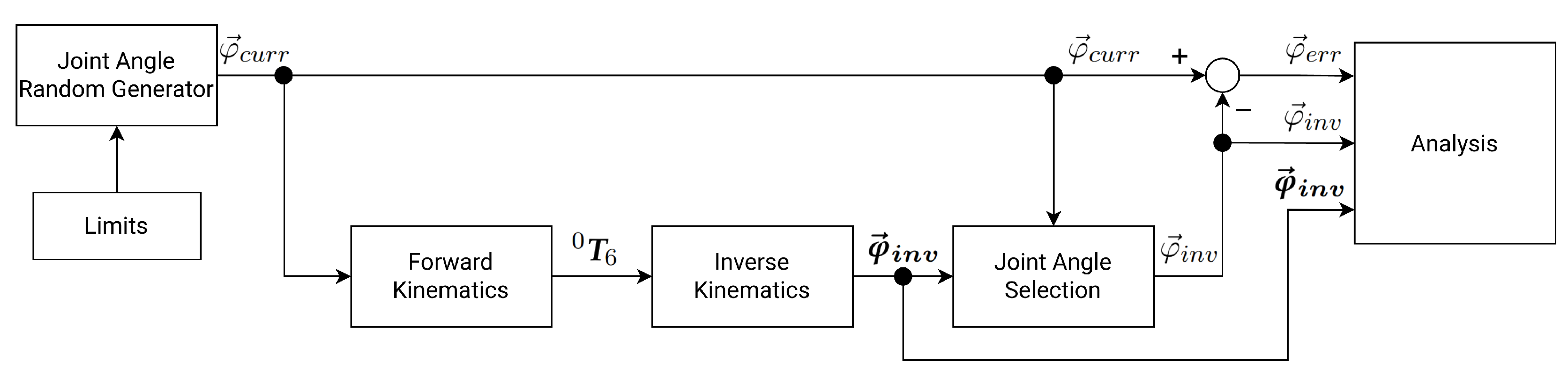
6.1. Evaluation and Test Procedure

To verify the solution of the inverse solver, a test procedure is defined and implemented in MATLAB^®. The test procedure (depicted in Figure 7) is as follows:

• Import the manipulator geometry and set the parameters described in Table 1.
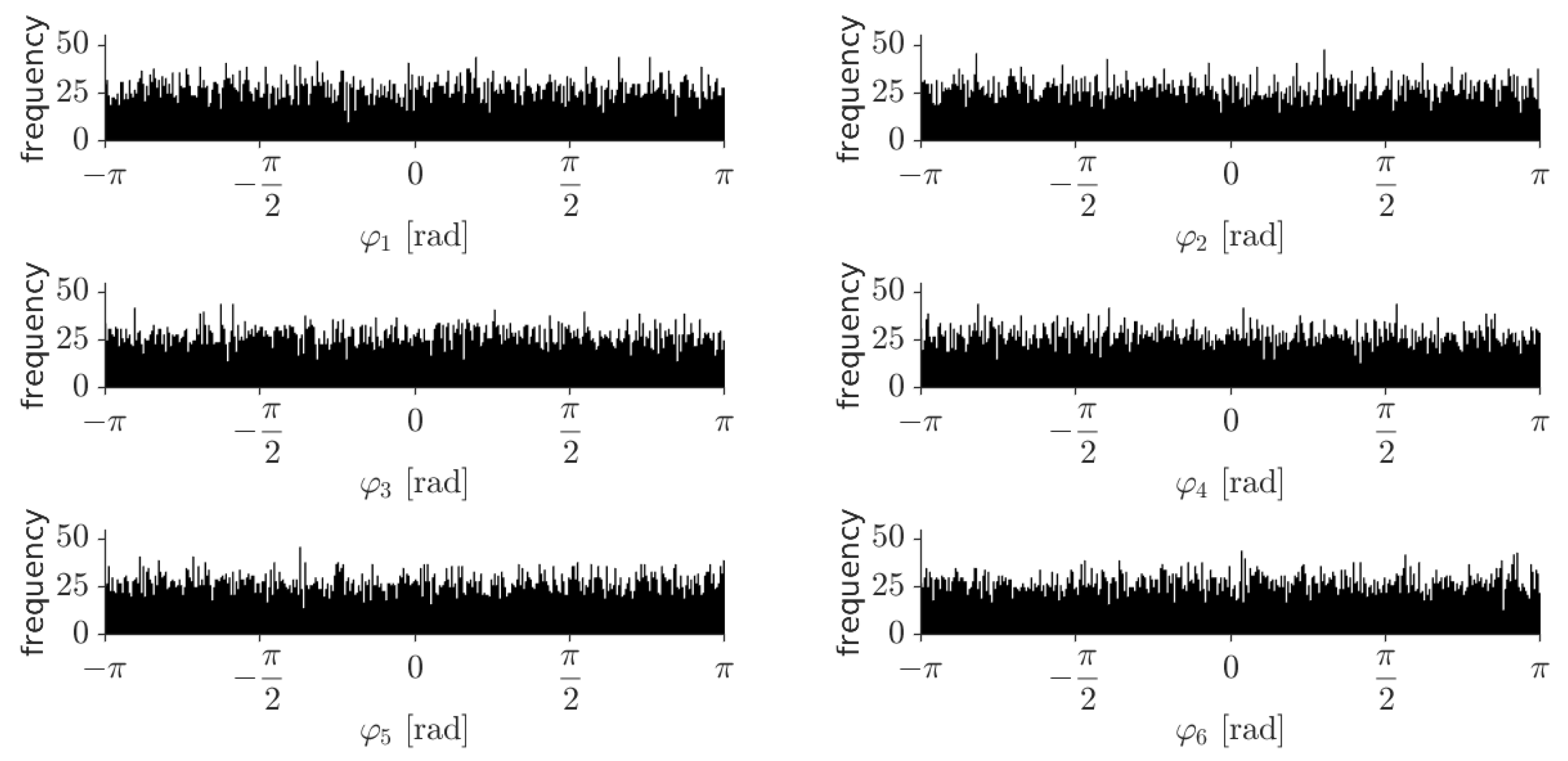
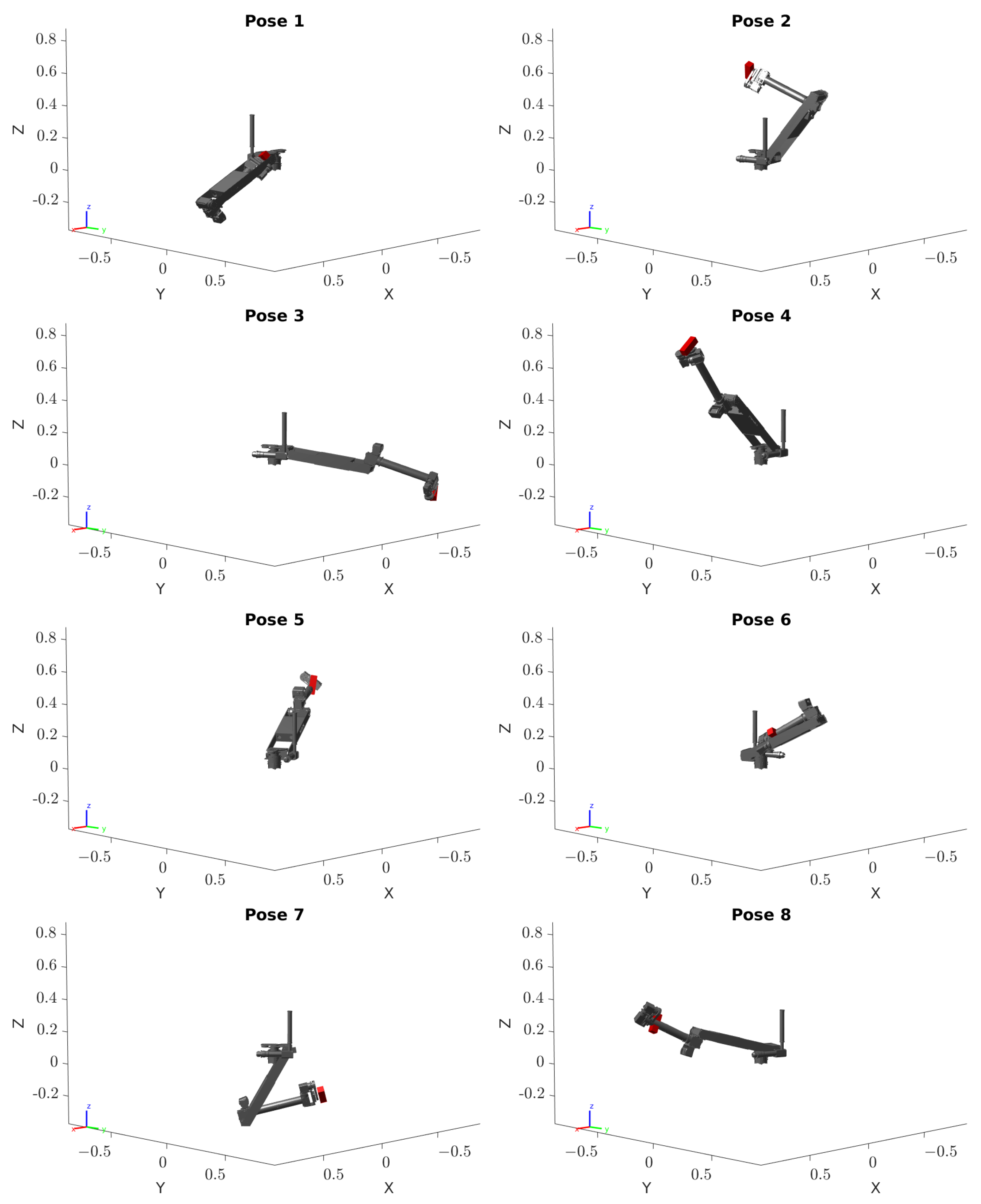
• Random generation of a combination of joint angles ${\phi }_1\dots {\phi }_6$ (${\overrightarrow{\phi }}_{curr}$) within the limits.
• Forward transformation of the generated joint angle combination to obtain the pose of the TCP represented by the transformation matrix ${}^0{\mathit{T}}_6$.
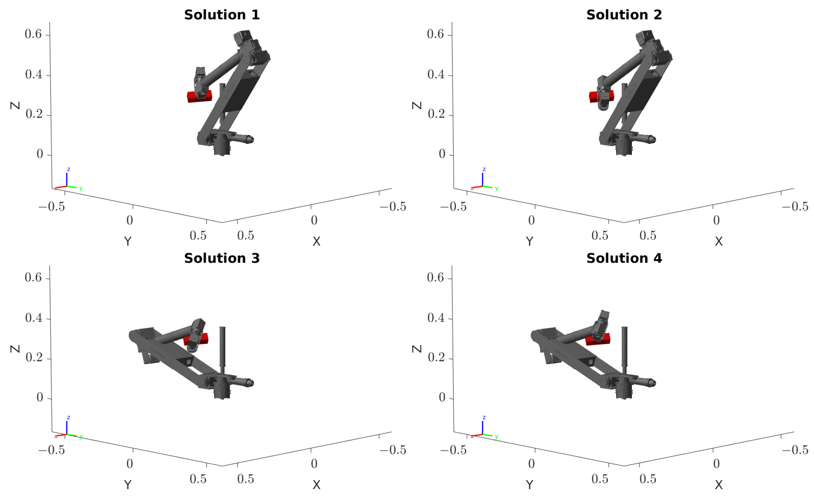
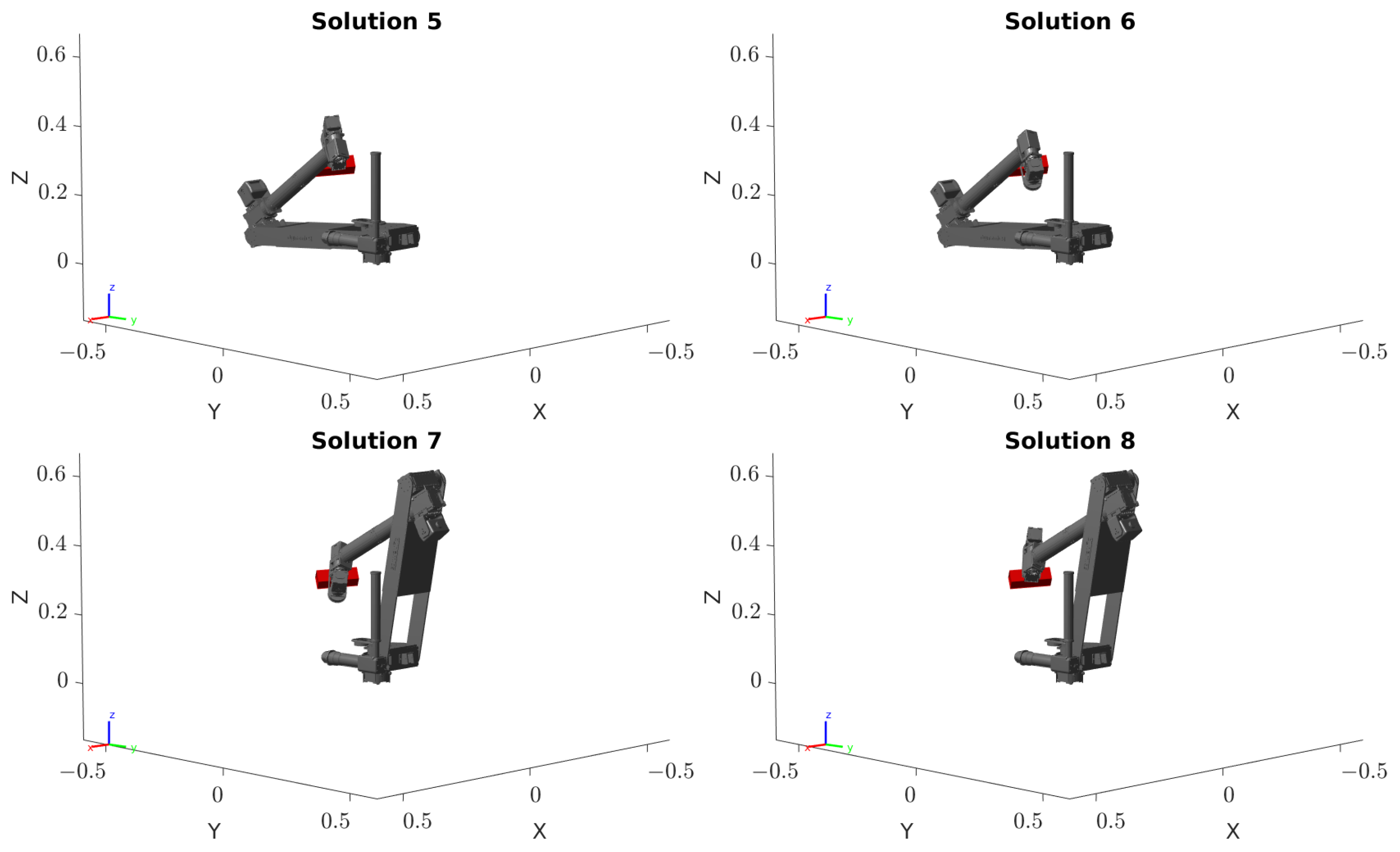
• Inverse transformation of the transformation matrix ${}^0{\mathit{T}}_6$ to resolve for eight different combinations of joint angles ${\phi }_1\dots {\phi }_6$ (${\overrightarrow{\mathit{\phi }}}_{\mathit{inv}}$).
• Selection of the combination of joint angles which causes the smallest angular deviation as the solution (${\overrightarrow{\phi }}_{inv}$).
• Analysis of the IK solution in comparison with the generated joint angles and the remaining joint angle combinations.

6.2. Selection of the Solution

As described in Section 5.1, a maximum of eight different solutions to the IK problem exist, each leading to the desired pose of the TCP. However, when using the solver in practice, only one of the eight solutions is important. It is reasonable to select the solution which results in the smallest angular difference with respect to the current joint angles. As a consequence, the joints of the manipulator move at a minimum to reach the goal pose.

The minimum joint motion can be determined by several approaches. The most straightforward approach is the one shown in Figure 7, where all eight possible combinations of joint angles are calculated and then the most suited solution is selected. Alternatively, the minimum joint motion can be obtained by considering the three subgroups of joints (described in Section 5.1). It is assumed that a minimum motion of each subgroup leads to a minimum total motion of the manipulator, which means that all subgroups can be considered separately. Since the smallest angle difference can be determined after each solved subgroup of joint angles, the desired combination of joint angles can be narrowed down after each subgroup. This approach corresponds to a fusion of the components Inverse Kinematics and Joint Angle Selection (cf. Figure 7). As a result, the desired combination of joint angles remains and moreover, the calculation effort can be considerably reduced.

The angular difference $\Delta {\phi }_j$ for each possible joint angle combination j of a subgroup can be calculated using Equation (49), where ${∆}_{inv,i}$ represents the IK solutions of joint $\left\{i\right\}$ and ${\phi }_{curr,i}$ represents the current angle of joint $\left\{i\right\}$. The joint indices k and l define the subgroup of joints, which is a subset of $\{1,\dots ,6\}$.

$$∆{\phi }_j=\sum _{i=k}^l|{\phi }_{inv,i,j}-{\phi }_{curr,i}|$$

(49)

Subsequently, the joint angle combination j with the smallest angular difference $∆{\phi }_j$ is selected as the solution.

In some cases, joint angle combinations can be excluded in advance, because, e.g., the joint limits are exceeded. For instance, in the case of the manipulator analyzed here, the elbow-down configurations are excluded due to the limits of joint $\left\{3\right\}$, i.e., only the elbow-up configurations of joint angles are relevant. Moreover, for combinations where the joint angles can be calculated independently, such as in Equations (45)–(47), a single joint angle may be sufficient to select the solution, which eliminates the need to calculate all joint angles of the subgroup. Hence, the calculation time may be further reduced.

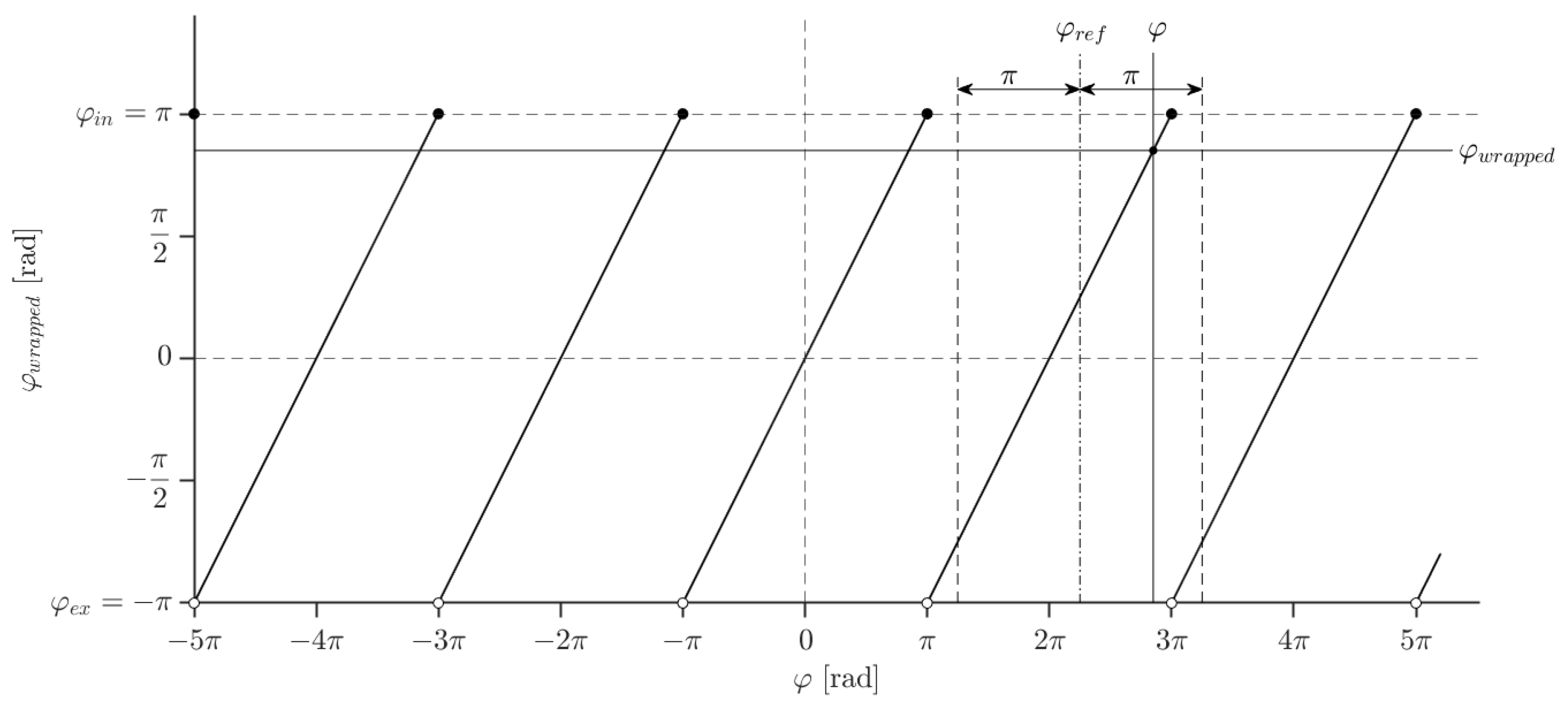
6.3. Conversion between Singleturn and Multiturn Range

For the calculation with joint angles, it is essential that angles can be transformed between multiturn range $[-\infty ,\infty ]$ and singleturn range (e.g., $[-\pi ,\pi ]$) while maintaining the position of the joint. These transformations are particularly necessary when using continuous rotational joints with angles exceeding the singleturn range. Moreover, the conversion to a specific range may be required after the addition or subtraction of joint angles, e.g., when calculating the joint angles of the elbow due to the angular offset ${\beta }_3$ or when calculating the difference of two joint angles in order to select a solution. Hence, the functions wrap() and unwrap() are defined. The function wrap() is used to convert the multiturn angle $\phi$ to the singleturn angle ${\phi }_{wrapped}$ (cf. Equation (50))

$${\phi }_{wrapped}=wrap(\phi ,{\phi }_{in},{\phi }_{ex}):=\phi -floor\left(\frac{\phi -{\phi }_{in}}{{\phi }_{ex}-{\phi }_{in}}\right)·({\phi }_{ex}-{\phi }_{in})$$

(50)

and the function unwrap() is used to transform the singleturn angle ${\phi }_{wrapped}$ to the multiturn angle $\phi$ using a reference angle ${\phi }_{ref}$ (cf. Equation (51)).

$$\phi =unwrap({\phi }_{wrapped},{\phi }_{ref},{\phi }_{in},{\phi }_{ex}):={\phi }_{ref}+wrap({\phi }_{wrapped}-{\phi }_{ref},{\phi }_{in},{\phi }_{ex})$$

(51)

In order to convert the angles, the range is set by means of the included angle ${\phi }_{in}$ and the excluded angle ${\phi }_{ex}$. For example, by setting ${\phi }_{in}$ to $\pi$ and ${\phi }_{ex}$ to $-\pi$, the angles are converted to the range $[-\pi ,\pi ]$. The reference angle ${\phi }_{ref}$ limits the possible multiturn range with the result that there remains only one valid solution. Hence, the maximum angular difference between the multiturn angle $\phi$ and the reference angle ${\phi }_{ref}$ is $\pi$. As a reference angle, e.g., the current joint angle ${\phi }_{curr}$ can be used. The functional principle of the conversion is depicted in Figure 8.

6.4. Singularities and Limits

Joint angles exist where the manipulator loses DOF due to its geometry, and these are commonly referred to as singularities of the manipulator. For singular configurations, there are often an infinite number of joint positions that lead to the same TCP pose. Furthermore, jump discontinuities of joint positions may occur for adjacent TCP poses near singularities. Due to the stated reasons, motions in the vicinity of singular configurations can cause unintended behavior, such as sudden joint rotations, and thus have to be considered separately.

In order to prevent critical behavior, the singularities of the manipulator have to be identified. Despite the fact that solutions for IK solvers based on geometric methods can be identified analytically, the calculation is performed numerically using computer-based systems. This causes the numerical errors to increase as the singular configurations are approached and can further lead to inaccurate results or, at worst, invalid floating point numbers (NaN) in the immediate vicinity of the singularities. If the required accuracy of the solver is known in advance, the numerical range for the identification of the singularities can be set more generously and thus the calculation of invalid solutions can be prevented.

The singularities and limits of the manipulator are considered separately for each of the three subgroups described in Section 5.1.

6.4.1. Joint 1

The singularity of joint $\left\{1\right\}$, also referred to as shoulder singularity, occurs when the WP lies on the rotation axis of joint $\left\{1\right\}$. A special case arises if, in addition, the rotation axes of joints $\left\{1\right\}$ and $\left\{6\right\}$ coincide. In the case of a shoulder singularity, the x and y components of the vector ${}^0{\overrightarrow{p}}_{05}$, stated in Equation (13), are zero and hence the joint angle ${\phi }_1$ is undefined and cannot be resolved (cf. Equation (14)). In order to avoid an undefined angle, a numerically small threshold is defined which is used to specify a small area on the $xy$-plane around the rotation axis of joint $\left\{1\right\}$. If this critical area is reached, i.e., the length of the vector ${\overrightarrow{p}}_{05}$ falls below the threshold, e.g., the current joint angle ${\phi }_{curr}$ can be selected as the solution or, alternatively, the angle ${\phi }_1$ can be calculated based on the goal orientation of the TCP and the current joint angles ${\phi }_{curr}$ of the wrist. Subsequently, the remaining joint angles can be calculated.

6.4.2. Joints 2 and 3

The elbow singularity occurs when the WP lies on the straight line through joints $\left\{2\right\}$ and $\left\{3\right\}$, i.e., the vectors ${\overrightarrow{p}}_{23}$ and ${\overrightarrow{p}}_{35}$ are collinear. Thereby, the elbow-up and elbow-down configurations degenerate to one singular configuration. This case can only occur when the manipulator is either fully unfolded or fully folded, although it is typically not physically possible to fully fold the manipulator due to collisions. The elbow singularity represents the exact limits of the domain of the functions stated in Equations (29) and (32). In the case of a singularity, the argument of the arc cosine function is either 1 or $-1$, which corresponds to an angle of 0 or $\pi$, respectively. Hence, the angles ${\phi }_2$ and ${\phi }_3$ can be resolved using Equations (30) and (33), with the numerical accuracy decreasing as the singularity is approached. Further research in this context is discussed in Section 6.5.

6.4.3. Joints 4, 5, and 6

The coincidence of the rotation axes of joints $\left\{4\right\}$ and $\left\{6\right\}$ is referred to as wrist singularity and occurs if the joint angle ${\phi }_5$ is equal to $k·\pi$ ($k\in \mathbb{Z}$). As a consequence, the angles ${\phi }_4$ and ${\phi }_6$ can no longer be resolved via the matrix entries stated in Equation (36) at singular configurations of the rotation matrix ${}^3{\mathit{R}}_6$ (cf. Equations (52) and (53)).

$$\begin{array}{c}\hfill {}^3{\mathit{R}}_6=Rot(x,{\phi }_4)·Rot(y,0)·Rot(x,{\phi }_6)=Rot(x,{\phi }_4)·\mathit{I}·Rot(x,{\phi }_6)=\hfill \\ \hfill Rot(x,{\phi }_4+{\phi }_6)=\left[\begin{array}{ccc}1& 0& 0\\ 0& cos({\phi }_4+{\phi }_6)& -sin({\phi }_4+{\phi }_6)\\ 0& sin({\phi }_4+{\phi }_6)& cos({\phi }_4+{\phi }_6)\end{array}\right]\end{array}$$

(52)

$$\begin{array}{c}\hfill {}^3{\mathit{R}}_6=Rot(x,{\phi }_4)·Rot(y,\pi )·Rot(x,{\phi }_6)=Rot(x,{\phi }_4)·Rot(y,-\pi )·Rot(x,{\phi }_6)=\hfill \\ \hfill \left[\begin{array}{ccc}-1& 0& 0\\ 0& cos({\phi }_4-{\phi }_6)& sin({\phi }_4-{\phi }_6)\\ 0& sin({\phi }_4-{\phi }_6)& -cos({\phi }_4-{\phi }_6)\end{array}\right]\end{array}$$

(53)

Singularities of the wrist can be detected via the matrix entry ${}^3{m}_{6,x}$, and subsequently, the corresponding joint angle ${\phi }_5$ can be set. For this purpose, a numerical threshold is defined, since it is very unlikely that the matrix entry ${}^3{m}_{6,x}$ is exactly 1 or $-1$. For the matrix entry ${}^3{m}_{6,x}$ reaching approximately 1, Equation (54) applies. For the matrix entry ${}^3{m}_{6,x}$ reaching approximately $-1$, an analogous procedure can be followed but shall not be further elaborated here since the findings are equivalent.

$$cos\left({\phi }_5\right)=1-threshold$$

(54)

Rearranging Equation (54) yields Equation (55) for calculating the numerical threshold in order to achieve a certain maximum angular deviation ${\phi }_{threshold}$ of the joint angle ${\phi }_5$.

$$threshold=1-cos\left({\phi }_{threshold}\right)$$

(55)

The relationship of the threshold and the maximum angular deviation ${\phi }_{threshold}$ is shown in the double logarithmic graph depicted in Figure 9.

For example, if a wrist singularity is to be detected at an angular deviation ${\phi }_{threshold}$ of joint angle ${\phi }_5$ smaller than one-tenth of a degree, the numerical threshold is to be set to

$$threshold=1-cos\left({0.1}^{°}\right)\approx 1.5\times {10}^{-6}.$$

(56)

In the case of a singularity, the joint angles ${\phi }_4$ and ${\phi }_6$ are calculated via the matrix entries ${}^3{n}_{6,y}$ and ${}^3{o}_{6,y}$ (cf. Equations (57)) due to the fact that the calculation is more efficient than using the matrix entries ${}^3{n}_{6,z}$ and ${}^3{o}_{6,z}$.

$$\begin{array}{cc}\hfill {}^3{n}_{6,y}& \hfill =n_y·C_1-n_x·S_1\hfill \\ \hfill {}^3{o}_{6,y}& \hfill =o_y·C_1-o_x·S_1\hfill \end{array}$$

(57)

Subsequently, Equation (58) is used to calculate the combination of the joint angles ${\phi }_4$ and ${\phi }_6$ based on the rotation matrix ${}^3{\mathit{R}}_6$ at singular configurations (cf. Equations (52) and (53)).

$$\begin{array}{cc}\hfill {\phi }_4+{\phi }_6& =atan2(-{}^3{o}_{6,y},{}^3{n}_{6,y})\hfill \\ \hfill {\phi }_4-{\phi }_6& =atan2({}^3{o}_{6,y},{}^3{n}_{6,y})=-atan2(-{}^3{o}_{6,y},{}^3{n}_{6,y})\hfill \end{array}$$

(58)

By rearranging Equation (58), the joint angle ${\phi }_6$ can be expressed as a function of the rotation matrix ${}^3{\mathit{R}}_6$ and the angle ${\phi }_4$ (cf. Equation (59)).

$${\phi }_6=\left\{\begin{array}{cc}atan2(-{}^3{o}_{6,y},{}^3{n}_{6,y})-{\phi }_4\hfill & \mathrm{if}{}^3{m}_{6,x}>(1-threshold)\hfill \\ atan2(-{}^3{o}_{6,y},{}^3{n}_{6,y})+{\phi }_4\hfill & \mathrm{if}{}^3{m}_{6,x}<(-1+threshold)\hfill \end{array}\right.$$

(59)

Hence, the joint angle ${\phi }_6$ can be calculated if the joint angle ${\phi }_4$ is set to an arbitrary angle, e.g., the current joint angle ${\phi }_{4,curr}$. The joint angle ${\phi }_5$ can be set according to the matrix entry ${}^3{m}_{6,x}$.

6.5. Workspace and Solvability

Due to the fact that the solver is based on an analytical algorithm, a (non-imaginary) solution exists only if the pose of the end-effector is within the workspace of the manipulator. This condition can be checked for any TCP pose. The WP, the angle ${\phi }_1$, and consequently the vector ${\overrightarrow{p}}_{25}$ can be calculated by using the goal pose of the TCP and the geometry of the manipulator (cf. Equation (19)). Furthermore, the vectors ${\overrightarrow{p}}_{23}$ and ${\overrightarrow{p}}_{35}$ are known (cf. Equations (20) and (21), respectively). Since these three vectors span a triangle, with only the length of the vector ${\overrightarrow{p}}_{25}$ being variable, the solvability constraints

$$\begin{array}{cc}\hfill ||{\overrightarrow{p}}_{25}||& \le ||{\overrightarrow{p}}_{23}||+||{\overrightarrow{p}}_{35}||\hfill \\ \hfill ||{\overrightarrow{p}}_{25}||& \le a_2+\sqrt{{a_3}^2+{d_4}^2}\hfill \end{array}$$

(60)

and

$$\begin{array}{cc}\hfill ||{\overrightarrow{p}}_{25}||& \ge \left|||{\overrightarrow{p}}_{23}||-||{\overrightarrow{p}}_{35}||\right|\hfill \\ \hfill ||{\overrightarrow{p}}_{25}||& \ge |a_2-\sqrt{{a_3}^2+{d_4}^2}|\hfill \end{array}$$

(61)

apply (cf. triangle inequality). Geometrically, this means that the distance between the coordinate systems $\left\{2\right\}$ and $\left\{5\right\}$ (WP) cannot be greater than the distance resulting from a maximum deflection of the manipulator and cannot be smaller than the difference of the links. In addition, it must be considered that although the manipulator can reach the maximum deflection, the folded position cannot be reached due to the collision of the links and the limitations of the joints. For this reason, the solvability constraint is adapted to

$$||{\overrightarrow{p}}_{25}||\ge \sqrt{{(a_2-d_4)}^2+{a_3}^2}.$$

(62)

Consequently, if the stated constraints are not fulfilled, there is no solution to the problem.

Although no solution can be found when the vector length is not within the limits and thus the position of the WP cannot be reached, the joint angles ${\phi }_2$ and ${\phi }_3$ can be calculated so that the vector ${\overrightarrow{p}}_{25}$ is oriented towards the WP. Subsequently, the remaining joint angles ${\phi }_4\dots {\phi }_6$ can be calculated and the resulting pose approximates the desired pose. At maximum deflection, the joint angles result in

$$\begin{array}{cc}\hfill {\phi }_2& =\pi -{\beta }_2=\pi -atan2({}^1{p}_{25,z},{}^1{p}_{25,x})\hfill \\ \hfill {\phi }_3& =\pi -{\beta }_3=\pi -arctan\left(\frac{a_3}{d_4}\right)\hfill \end{array}$$

(63)

and the folded position exhibits the joint angles

$$\begin{array}{cc}\hfill {\phi }_2& =\pi -{\beta }_2-arctan\left(\frac{a_3}{|a_2-d_4|}\right)=\pi -atan2({}^1{p}_{25,z},{}^1{p}_{25,x})-arctan\left(\frac{a_3}{|a_2-d_4|}\right)\hfill \\ \hfill {\phi }_3& =0\hfill \end{array}$$

(64)

(see Figure 6). This allows the calculation of the joint angles for TCP poses outside the workspace of the manipulator.

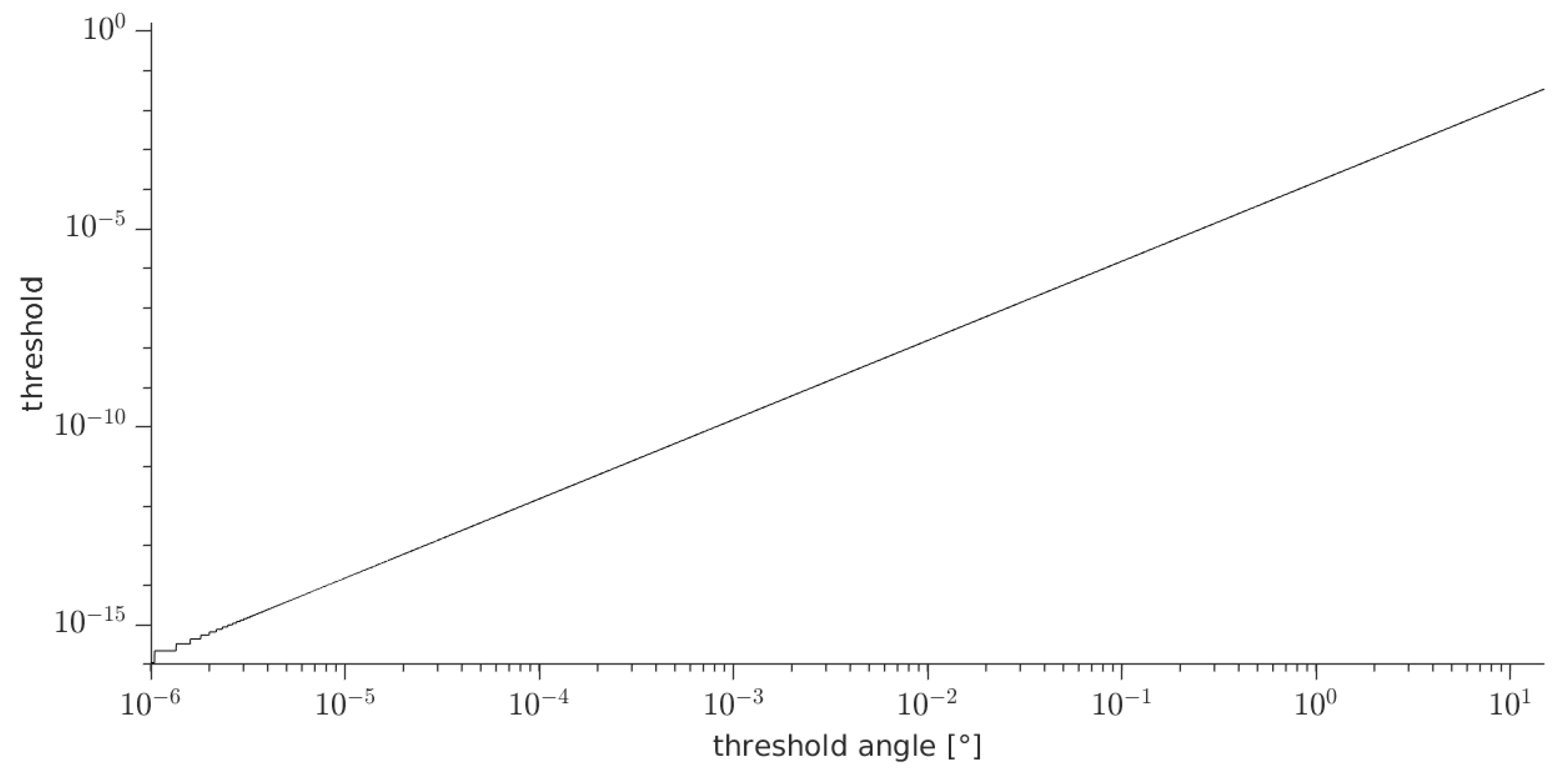
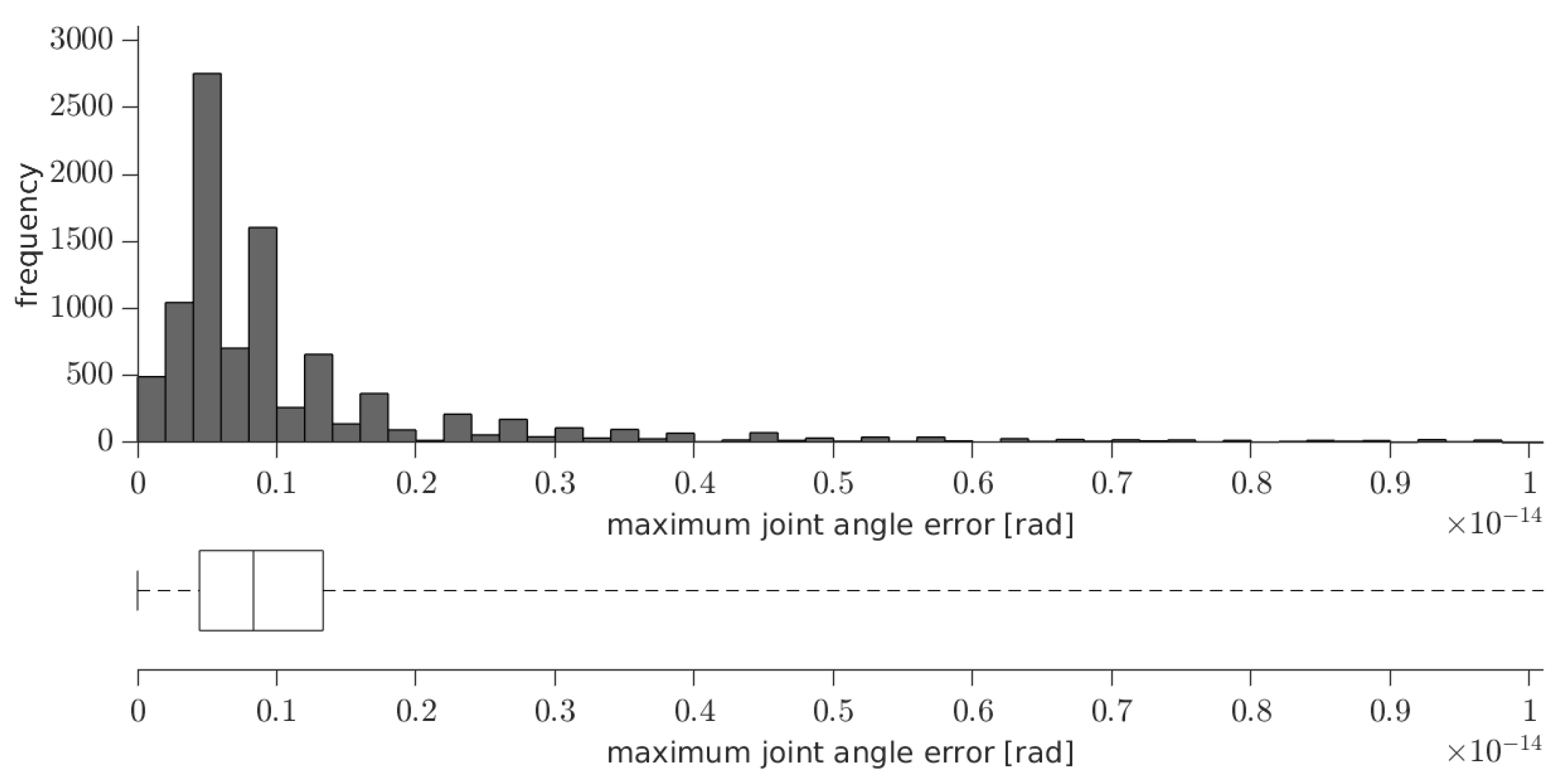
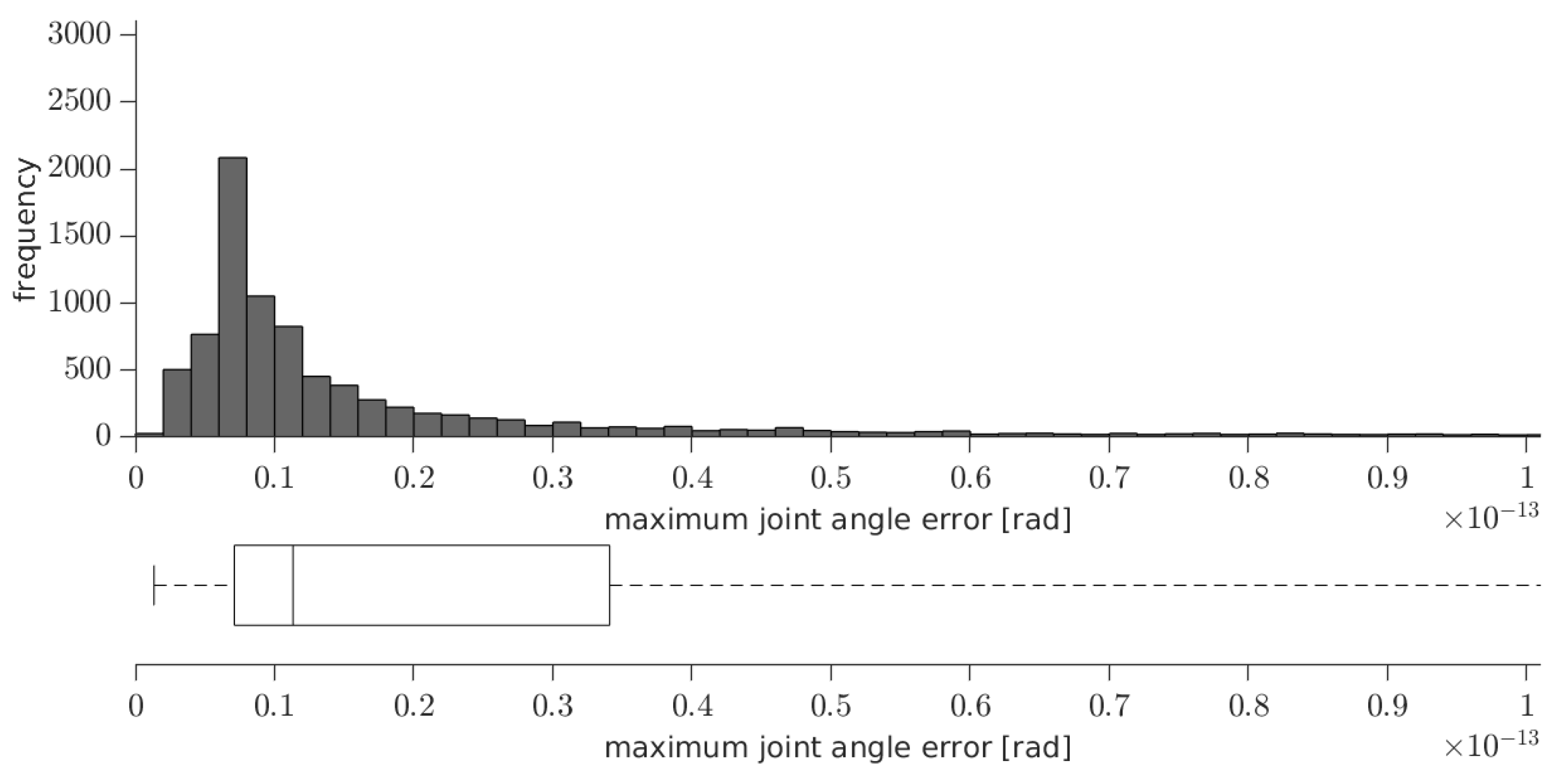
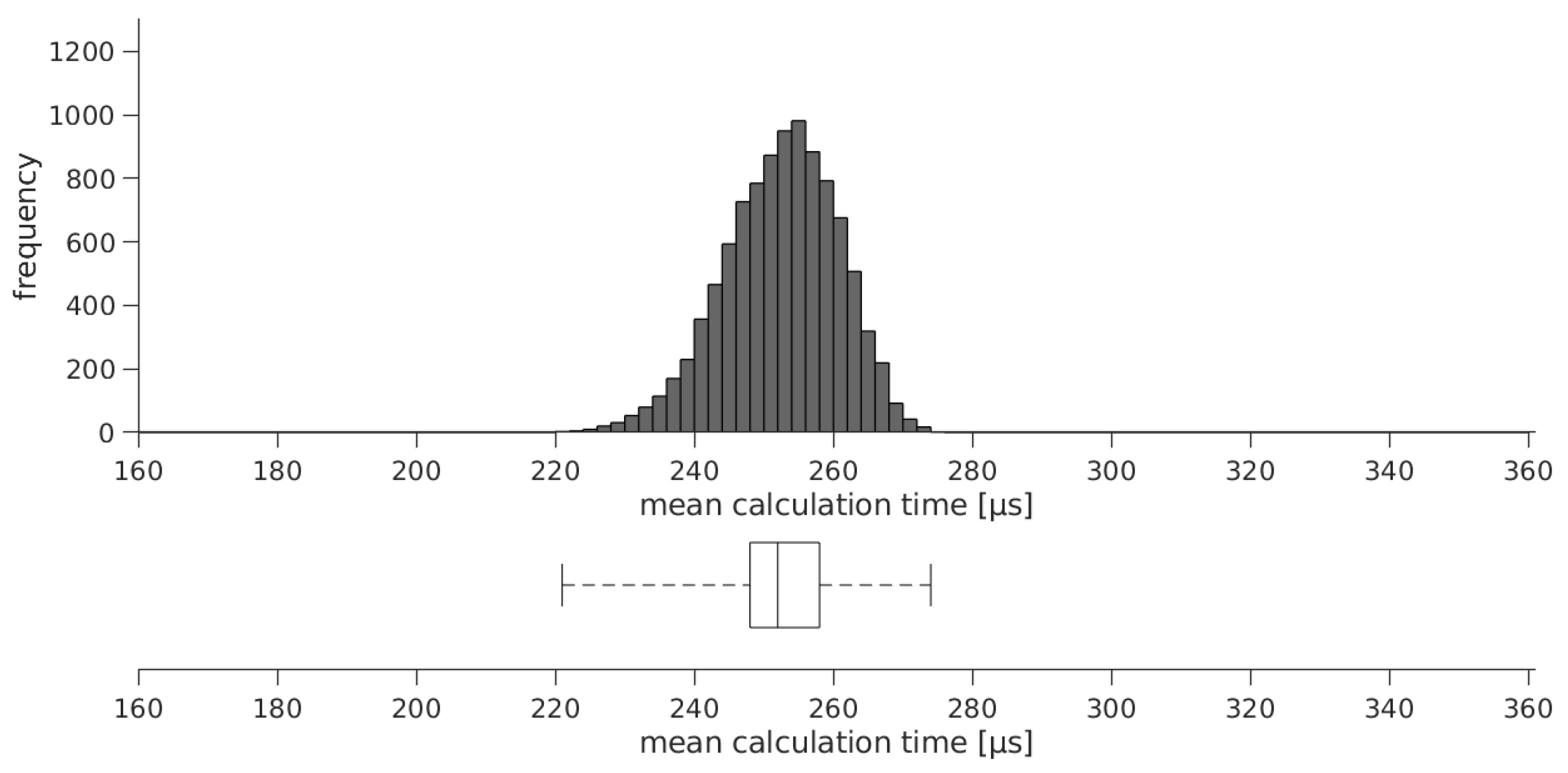
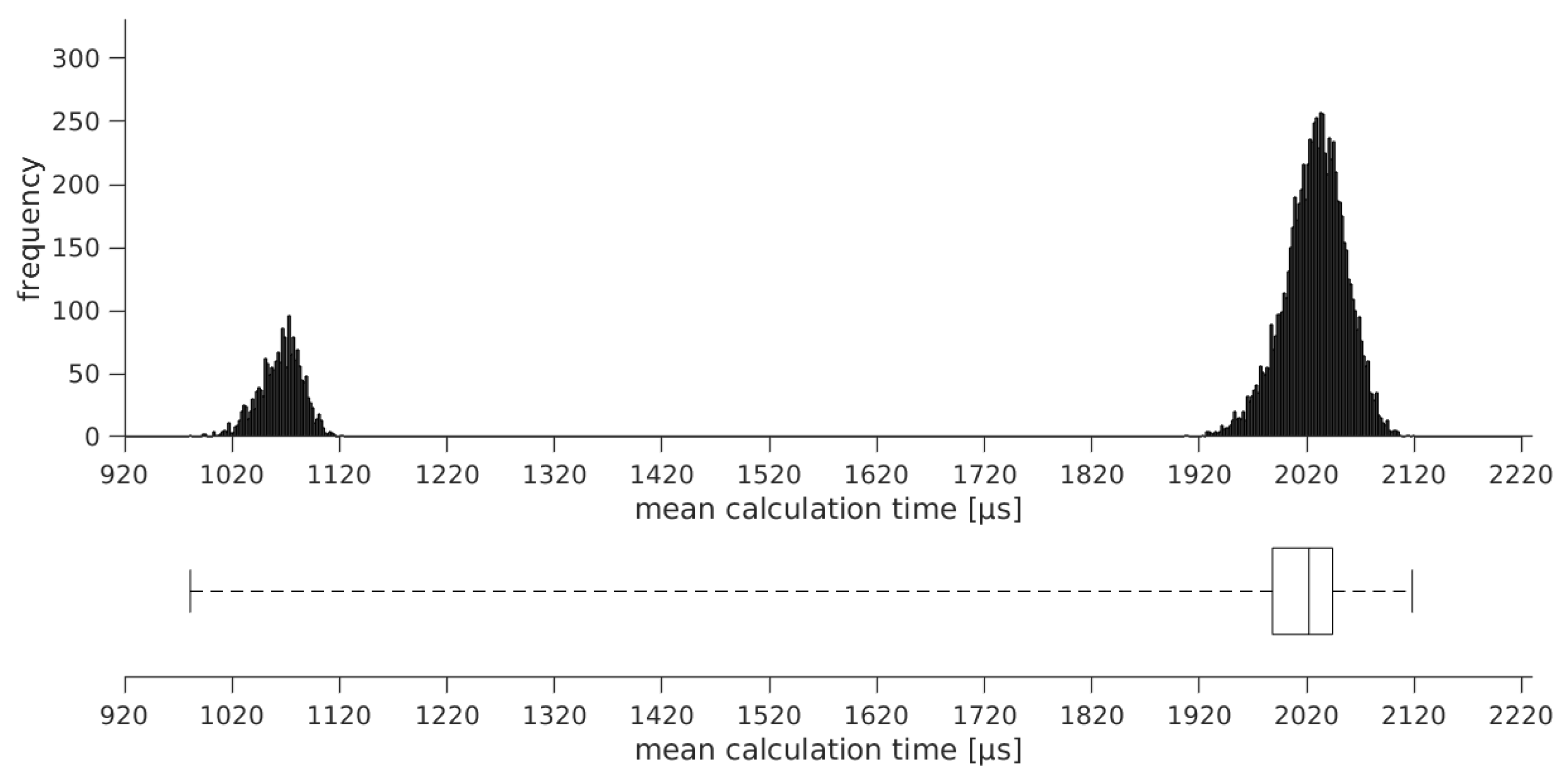
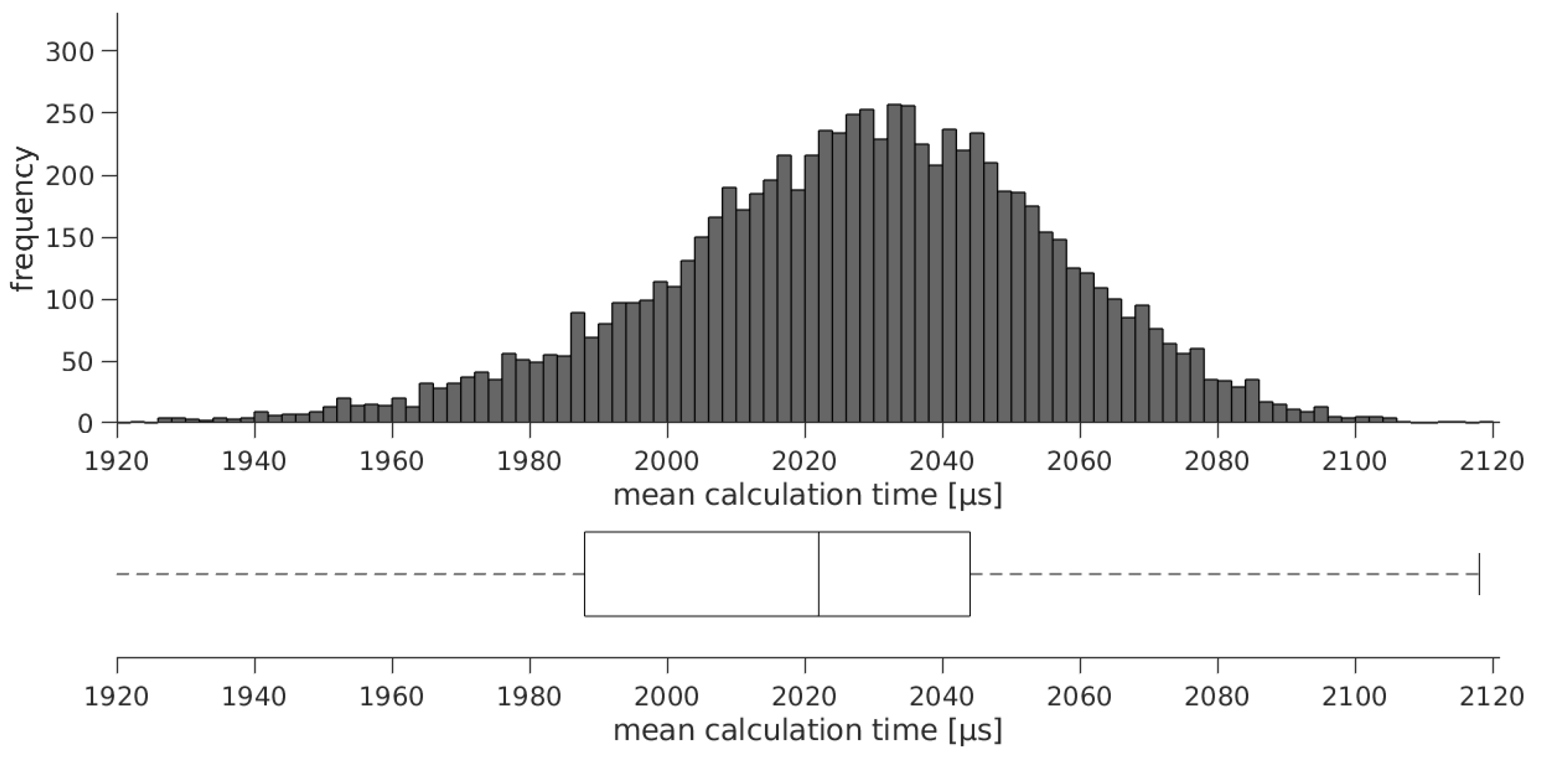
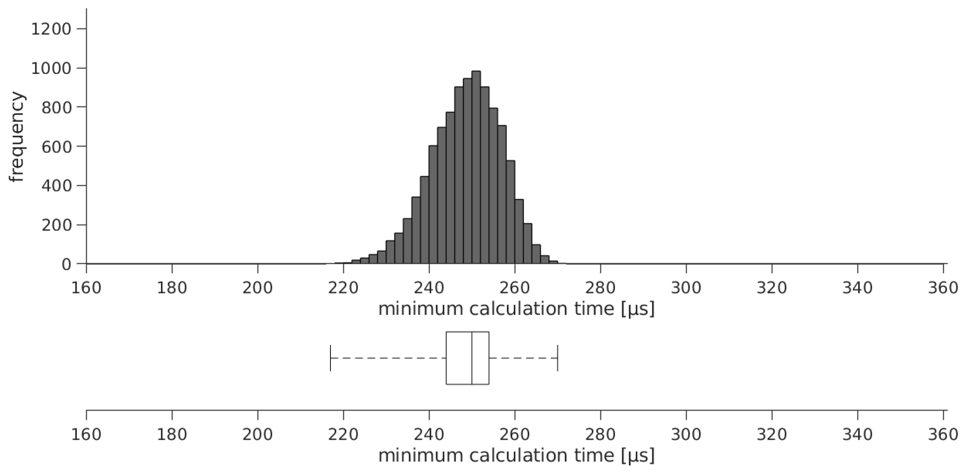
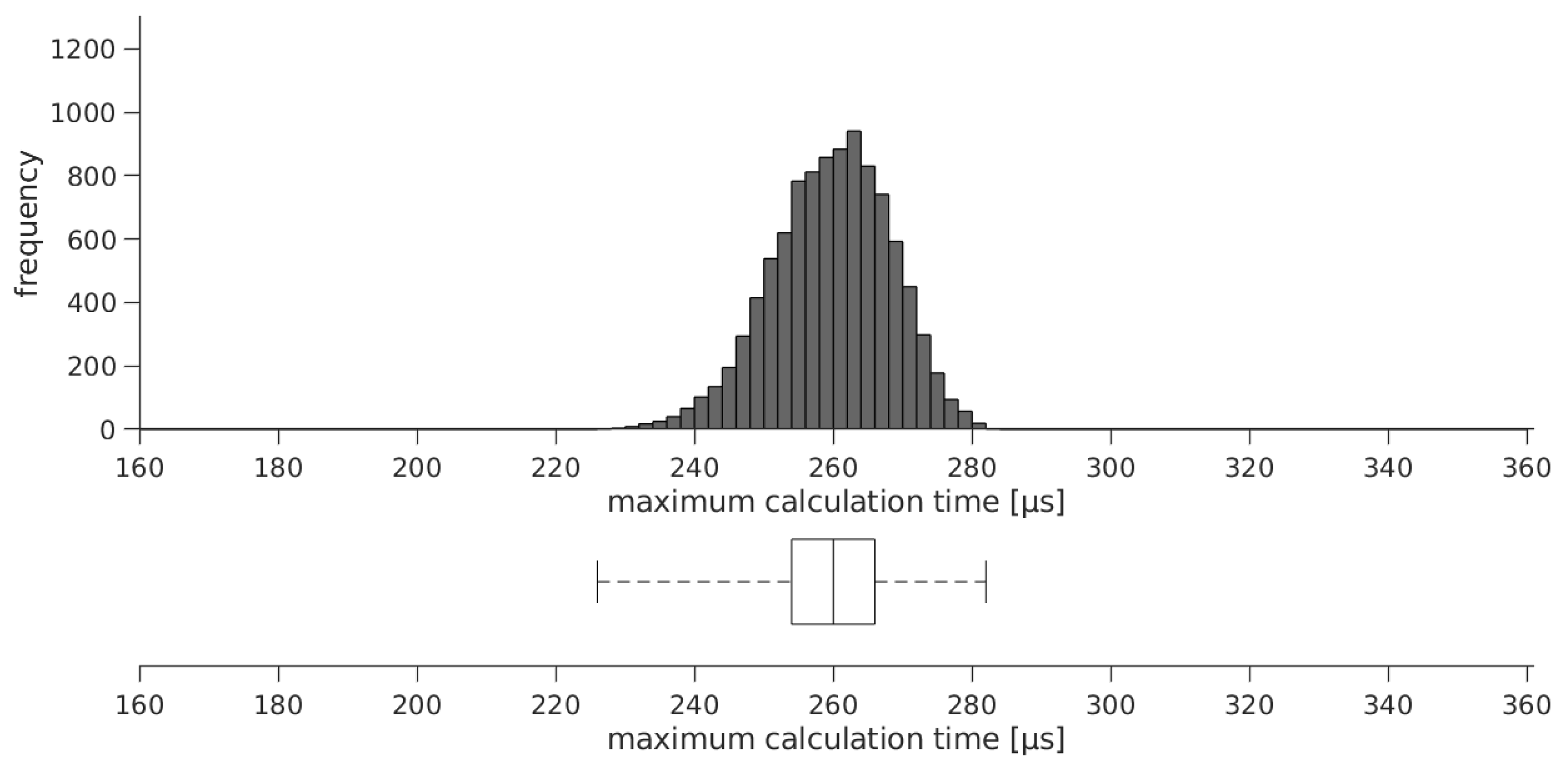
6.6. Solver Accuracy and Execution Time

The inverse solver consisting of the equations presented in Section 5 is simulated according to the test procedure described in Section 6.1. The TCP poses ${}^0{\mathit{T}}_6$ are generated by forward transformation of randomly generated joint angles ${\overrightarrow{\phi }}_{curr}$ within the range $[-\pi ,\pi ]$. Physical constraints of the manipulator such as collisions and joint limits are ignored, as only the mathematical capabilities of the solver are examined, thus all TCP poses within the workspace of the manipulator are evaluated. In addition, all eight combinations of joint angles ${\overrightarrow{\mathit{\phi }}}_{\mathit{inv}}$ are calculated (cf. Figure A1 and Figure A2 in Appendix A). However, only the solution ${\overrightarrow{\phi }}_{inv}$ with the smallest angle difference is considered in the evaluation, which is determined on the basis of the joint angles ${\overrightarrow{\phi }}_{curr}$ (cf. Equation (49)). In order to obtain representative results, a data set of m = 10,000 randomly generated joint angle combinations is created. Consequently, valid solutions exist for each combination. The generated data set consisting of the joint angles ${\phi }_1\dots {\phi }_6$ is approximately uniformly distributed (illustrated in the histograms in Figure 10).

To evaluate the capability and accuracy of the inverse solver, the following solver variants based on

• Equations (14), (30), (33) and (42)–(44);
• Equations (14), (30), (33) and (45)–(47); and
• Equations (14), (30), (33), (45), (47) and (48)

are examined. The detection of singularities, described in Section 6.4, is disabled, i.e., the threshold for the detection of shoulder and wrist singularities is set to zero. The solver variants are both simulated on PC and tested with the embedded board using the implicit and explicit equations. For the explicit calculation variants, the explicit equations derived in Section 5.1 are used, whereas for the implicit calculation variants, the stated matrix multiplications are calculated and then the resulting matrix entries are substituted into the equations. To compare the presented solver with the analytical solver IKFast, the source code of IKFast is generated based on the geometry of the manipulator, exported, and adapted for use on the embedded board. In order to obtain comparable results, the identical, randomly generated data set depicted in Figure 10 is both used for the simulation and the evaluation of the inverse solver. The data are transmitted without loss of numerical precision. After executing steps 3 to 5 of the test procedure (cf. Section 6.1) on the embedded board, the results are transferred to the PC for further analysis.

The capability and accuracy of the solver are evaluated based on the maximum joint angle error ${\phi }_{err,max}$ for each combination j of all $n=6$ joints (cf. Equation (65)). The desired result is to exactly resolve the joint angles ${\overrightarrow{\phi }}_{curr}$, i.e., the angular difference to the resolved joint angles ${\overrightarrow{\phi }}_{inv}$ expressed with the joint angle errors ${\overrightarrow{\phi }}_{err}$ is zero and thus the desired maximum joint angle error ${\phi }_{err,max}$ is zero.

$${\phi }_{err,max}=max\left({\overrightarrow{\phi }}_{err}\right)=max|{\overrightarrow{\phi }}_{curr}-{\overrightarrow{\phi }}_{inv}|=\underset{i=1}{\overset{n}{max}}|{\phi }_{curr,i}-{\phi }_{inv,i}|$$

(65)

The histogram and the associated box plot of the maximum joint angle error ${\phi }_{err,max}$ using the solver variant 2 with explicit equations are depicted in Figure 11 (calculated with MATLAB^® on the PC) and Figure 12 (calculated with the embedded board). The histogram and the associated box plot of the maximum joint angle error ${\phi }_{err,max}$ of IKFast executed on the embedded board are depicted in Figure 13 (note the different scaling of the x-axis).

For further examination, all solver variants are tested and examined. The histograms of the remaining variants 1 and 3 present the same course as the histograms shown in Figure 11 and Figure 12. Due to the fact that the histograms represent an irregular distribution with a wide value range, the percentiles of the distribution of the maximum joint angle errors ${\phi }_{err}$, shown in

Table 3. Percentiles of the distribution of the maximum joint angle errors ${\phi }_{err}$.

Solver Variant			Percentile [ ${10}^{-16}$ $\mathbf{rad}$]
			0th (Min.)	5th	25th	50th (Med.)	75th	95th	99th	100th (Max.)
PC	implicit	1	0.0	2.2	4.4	8.9	17.8	125.4	770.5	107,642.8
		2	0.0	2.2	4.4	8.9	17.8	125.5	770.5	107,642.8
		3	0.0	2.2	4.4	8.9	17.8	127.4	783.3	107,642.8
	explicit	1	0.0	2.2	4.4	7.8	13.3	102.1	532.8	309,219.3
		2	0.0	2.2	4.4	8.3	13.3	102.1	532.8	309,219.3
		3	0.0	2.2	4.4	8.9	15.5	106.6	537.3	309,219.3
Embedded Board	implicit	1	0.0	2.2	4.4	8.9	14.4	102.1	562.3	267,226.2
		2	0.0	2.2	4.4	8.9	14.4	102.1	562.3	267,226.2
		3	0.0	2.2	4.4	8.9	15.5	106.6	579.5	267,226.2
	explicit	1	0.0	2.2	4.4	8.9	14.4	102.1	532.8	309,219.3
		2	0.0	2.2	4.4	8.9	14.4	102.1	532.8	309,219.3
		3	0.0	2.2	4.4	8.9	15.5	106.6	532.8	309,219.3
	IKFast		13.3	40.0	71.1	113.2	340.8	3466.1	20,643.5	24,375,716.2

, are used for the characterization.

For further investigation, the mean calculation time ${\overline{t}}_{mean}$ of the presented solver variants and IKFast are compared to the average joint angle error ${\overline{\phi }}_{err}$. For this purpose, the calculation on the embedded board is repeated $k=100$ times for each joint angle combination j. The required calculation time $t_l$ is measured for each repetition l with a resolution of $1 \mathsf{\mu }\mathrm{s}$. Subsequently, the average, minimum, and maximum calculation times $t_{mean}$, $t_{min}$, and $t_{max}$ of each joint angle combination are determined. The calculation times for variant 2 are depicted in Figure 14 and in Figure A4 and Figure A5 in Appendix B. Variant 2 is shown as a representative of all solver variants, which show similar normally distributed courses. The calculation times for IKFast are depicted in Figure 15, and the interesting area is enlarged and depicted in Figure 16.

An overall arithmetic mean value ${\overline{t}}_{mean}$ of all m = 10,000 combinations is calculated from the arithmetic mean values $t_{mean}$ in order to obtain a reasonable parameter for the comparison of the solver variants (cf. Equation (66)).

$${\overline{t}}_{mean}=\frac{1}{m}\sum _{j=1}^m{t}_{mean}=\frac{1}{m·k}\sum _{j=1}^m\sum _{l=1}^k{t}_l$$

(66)

The average joint angle error is obtained via the arithmetic mean of all joint angle errors of all combinations and is calculated according to Equation (67), where the joint index i runs from one to the maximum number of joints $n=6$ for each combination j running from one to the number of m = 10,000 combinations.

$${\overline{\phi }}_{err}=\frac{1}{m·n}\sum _{j=1}^m\sum _{i=1}^n{\phi }_{err,i,j}=\frac{1}{m·n}\sum _{j=1}^m\sum _{i=1}^n|{\phi }_{curr,i,j}-{\phi }_{inv,i,j}|$$

(67)

The results of the average calculation time stated in Equation (66) and the average joint angle error stated in Equation (67) are compared in

Table 4. Average joint angle error ${\overline{\phi }}_{err}$ and average calculation times ${\overline{t}}_{mean}$ on the embedded board.

Solver Variant		PC	Embedded Board
		${\overline{\mathit{\phi }}}_{\mathit{err}}$ [ ${10}^{-15}$ $\mathbf{rad}$]	${\overline{\mathit{\phi }}}_{\mathit{err}}$ [ ${10}^{-15}$ $\mathbf{rad}$]	${\overline{\mathit{t}}}_{\mathit{mean}}$ [$\mathbf{\mu }\mathbf{s}$]
implicit	1	2.86	3.05	378.3
	2	2.86	3.05	313.7
	3	2.93	3.13	310.1
explicit	1	3.16	3.19	316.1
	2	3.16	3.20	252.0
	3	3.24	3.27	252.9
IKFast		-	153.99	1856.2

.

7. Discussion

Based on the histograms and box plots depicted in Figure 11 and Figure 12, which cover the majority of the data, no difference in accuracy between the simulation and the execution on the embedded board can be observed for solver variant 2 (the histograms and box plots of the solver variants 1 and 3 show an analogous course). Moreover, it can be observed that the majority of the joint angle combinations exhibit a minor joint angle error. On the basis of the percentiles stated in Table 3, it can be determined that 99% of the joint angle combinations exhibit a maximum error below ${10}^{-13}$ $\mathrm{rad}$ (cf. 99th percentile in Table 3). In the worst case, the maximum error is less than ${10}^{-10}$ $\mathrm{rad}$ (cf. 100th percentile in Table 3). Hence, it can be concluded that the presented solution is valid and moreover that the inverse solver is sufficiently accurate.

Furthermore, it can be seen that there is no significant numerical degradation due to the different variants since all variants exhibit similar results at the examined percentiles of the maximum joint angle errors. Additionally, it can be shown that the solver provides similarly accurate results both when simulated on the PC and when deployed on the embedded board.

Compared to IKFast, the presented solver variants show significantly lower error (cf. Table 3). The error of IKFast is more than ten times as large as that of the geometric solvers over the entire range of values, and the maximum error is at least more than eighty times greater (depending on the solver variant). This trend can be confirmed when comparing the histograms and box plots depicted in Figure 11, Figure 12 and Figure 13 (note the different scaling of the x-axis).

In Table 4, it can be observed that the average joint angle error of the calculation on the embedded board is slightly greater than the average joint angle error compared to the simulation on the PC. Hence, the solutions are slightly less accurate when calculated on the embedded board than the simulation results calculated on the PC. The largest joint angle errors are caused by poses in the vicinity of singularities (cf. Figure A3 in Appendix A). Moreover, the explicitly calculated variants exhibit a higher average error than the implicitly calculated variants. In addition, the error of variant 3 is greater compared to the other variants, with variants 1 and 2 having similar joint angle errors.

Furthermore, it can be observed that the average calculation times of the explicitly calculated variants are considerably lower than those of the implicitly calculated variants (cf. Table 4). In addition, a significant reduction of the average calculation time can be achieved with variants 2 and 3 compared to variant 1, whereas the average calculation times of variants 2 and 3 are approximately the same.

The average joint angle error ${\overline{\phi }}_{err}$ shows that the presented algorithm achieves significantly more accurate results than IKFast (cf. Table 4). However, the greatest achievement becomes clear when comparing the average calculation times ${\overline{t}}_{mean}$. It can be shown that the presented algorithm provides a considerably faster calculation of the solution in every case. Moreover, the presented algorithm provides more predictable calculation times due to the fact that the values are located in a more condensed range (cf. Figure 14, Figure 15 and Figure 16).

In summary, the solver variant 2 exhibits a low average calculation time in combination with a low average joint angle error and therefore combines the advantages of the different solver variants. The average joint angle error can be minimized by using the implicit calculation variants at the expense of higher calculation times, otherwise, the explicit calculation variants are sufficiently accurate. The proposed algorithm is suitable for use on embedded systems due to the real-time capability (cf. Figure A5 in Appendix B) and furthermore requires significantly less computation time than alternative algorithms such as IKFast. In addition, the accuracy of the solver is noticeably better than using IKFast.

8. Conclusions and Future Work

IK is the process of determining the joint angles of a robot manipulator that correspond to a desired end-effector position and orientation. This is a fundamental problem in robotic control, as it allows the manipulator to move to a desired location in the workspace. However, solving the IK problem can be computationally expensive and time-consuming, especially for complex robot manipulators with a high number of DOF.

One solution to this problem is to use a geometric approach for solving the IK of a 6R robot manipulator. In this approach, a geometric relationship between the end-effector and the joints of the manipulator is utilized to solve the IK problem. Thus, the algorithm can be simplified compared to analytical approaches. As a result, this method is computationally efficient and can be implemented on embedded boards in real-time, which makes it suitable for a wide range of mobile robotic applications. The proposed method is based on the following steps:

• The geometric relationship between the end-effector and the joints of the manipulator is established.
• The end-effector pose is expressed in terms of the joint angles of the manipulator.
• The IK problem is solved using this geometric relationship.

The effectiveness of the proposed method is demonstrated through simulation and experimental results. The simulation results show that the proposed method can accurately determine the joint angles of the manipulator for a wide range of end-effector positions and orientations. The experimental results show that the proposed method can be implemented in real-time and can be used to control the 6R robot manipulator to move to a desired location in the workspace. Compared to universal out-of-the-box solutions such as IKFast, the computation time can be significantly reduced and the accuracy of the solver can be noticeably improved. In summary, the proposed method provides an efficient and accurate solution to the IK problem for an anthropomorphic 6R robot manipulator with a spherical wrist.

The developed manipulator software framework will be crucial for developing safer and more powerful mobile manipulation tasks that can operate effectively in human environments in the future. Further algorithms which provide distance-checking capabilities that should generate collision detection and avoidance are a major goal. In addition, another significant milestone is to develop a differential kinematic algorithm in order to establish the relationship between the velocity of the TCP and the joint velocities. Furthermore, investigations concerning path and trajectory planning are to be conducted in order to achieve a smooth movement of the TCP. These measures are primarily intended to intuitively enable teleoperated control of the manipulator to perform a variety of handling and inspection tasks to be accomplished in the field of rescue robotics. As a result, safe, controllable, and efficient motions of the manipulator in space should be achieved.

In conclusion, the integration of the platform-independent IK solver presents a promising avenue for achieving efficient and optimized motion trajectories in robotic manipulators. The proposed framework provides a foundation for future research and development in the field of motion planning for robotic systems on embedded platforms.

References

1. Edlinger, R.; Nuechter, A. Marc-modular autonomous adaptable robot concept. In Proceedings of the 2019 IEEE International Symposium on Safety, Security, and Rescue Robotics (SSRR), Würzburg, Germany,, 2–4 September 2019; pp. 1–7. [Google Scholar]
2. Edlinger, R.; Anschober, M.; Froschauer, R.; Nüchter, A. Intuitive HRI Approach with Reliable and Resilient Wireless Communication for Rescue Robots and First Responders. In Proceedings of the 2022 31st IEEE International Conference on Robot and Human Interactive Communication (RO-MAN), Napoli, Italy, 29 August–2 September 2022; pp. 75–82. [Google Scholar]
3. Pieper, D.L. The Kinematics of Manipulators under Computer Control; Stanford University: Stanford, CA, USA, 1969. [Google Scholar]
4. Lee, C.S.G.; Ziegler, M. Geometric Approach in Solving Inverse Kinematics of PUMA Robots. IEEE Trans. Aerosp. Electron. Syst. 1984, AES-20, 695–706. [Google Scholar] [CrossRef]
5. Lloyd, J.; Hayward, V. Kinematics of common industrial robots. Robot. Auton. Syst. 1988, 4, 169–191. [Google Scholar] [CrossRef]
6. Raghavan, M.; Roth, B. Kinematic analysis of the 6R manipulator of general geometry. In Proceedings of the Fifth International Symposium on Robotics Research, Tokyo, Japan, 28–31 August 1989; pp. 314–320. [Google Scholar]
7. Denavit, J.; Hartenberg, R.S. A kinematic notation for lower-pair mechanisms based on matrices. ASME J. Appl. Mech. 1955, 22, 215–221. [Google Scholar] [CrossRef]
8. Manocha, D.; Canny, J.F. Efficient inverse kinematics for general 6R manipulators. IEEE Trans. Robot. Autom. 1994, 10, 648–657. [Google Scholar] [CrossRef] [Green Version]
9. Kucuk, S.; Bingul, Z. The inverse kinematics solutions of industrial robot manipulators. In Proceedings of the IEEE International Conference on Mechatronics, ICM‘04, Istanbul, Turkey, 5 June 2004; pp. 274–279. [Google Scholar] [CrossRef]
10. Husty, M.L.; Pfurner, M.; Schröcker, H.P. A new and efficient algorithm for the inverse kinematics of a general serial 6R manipulator. Mech. Mach. Theory 2007, 42, 66–81. [Google Scholar] [CrossRef]
11. Brandstötter, M.; Angerer, A.; Hofbaur, M. An Analytical Solution of the Inverse Kinematics Problem of Industrial Serial Manipulators with an Ortho-parallel Basis and a Spherical Wrist. In Proceedings of the Austrian Robotics Workshop, Linz, Austria, 22–23 May 2014. [Google Scholar]
12. Khatamian, A. Solving Kinematics Problems of a 6-DOF Robot Manipulator. Int. Conf. Sci. Comput. 2015, 2, 228. [Google Scholar]
13. Asif, S.; Webb, P. Kinematics analysis of 6-DoF articulated robot with spherical wrist. Math. Probl. Eng. 2021, 2021, 6647035. [Google Scholar] [CrossRef]
14. Pratheep, V.; Chinnathambi, M.; Priyanka, E.; Ponmurugan, P.; Thiagarajan, P. Design and Analysis of six DOF robotic manipulator. In Proceedings of the IOP Conference Series: Materials Science and Engineering; IOP Publishing: Erode, India, 2021; Volume 1055, p. 012005. [Google Scholar]
15. Zhang, H.; Xia, Q.; Sun, J.; Zhao, Q. A Fully Geometric Approach for Inverse Kinematics of a Six-Degree-of-Freedom Robot Arm. J. Phys. Conf. Ser. 2022, 2338, 012089. [Google Scholar] [CrossRef]
16. Dikmenli, S. Forward & Inverse Kinematics Solution of 6-DOF Robots Those Have Offset & Spherical Wrists. Eurasian J. Sci. Eng. Technol. 2022, 3, 14–28. [Google Scholar]
17. Krishnan, M.G.; Ashok, S. Kinematic Analysis and Validation of an Industrial Robot Manipulator. In Proceedings of the TENCON 2019—2019 IEEE Region 10 Conference (TENCON), Kochi, India, 17–20 October 2019; pp. 1393–1399. [Google Scholar] [CrossRef]
18. Chen, I.M.; Gao, Y. Closed-form inverse kinematics solver for reconfigurable robots. In Proceedings of the Proceedings 2001 ICRA. IEEE International Conference on Robotics and Automation (Cat. No.01CH37164), Seoul, Republic of Korea, 21–26 May 2001; Volume 3, pp. 2395–2400. [Google Scholar] [CrossRef]
19. Tab, Y.; Xiao, A. Extension of the Second Paden-Kahan Sub-problem and its’ Application in the Inverse Kinematics of a Manipulator. In Proceedings of the 2008 IEEE Conference on Robotics, Automation and Mechatronics, Chengdu, China, 21–24 September 2008; pp. 379–381. [Google Scholar] [CrossRef]
20. Chen, Q.; Zhu, S.; Zhang, X. Improved Inverse Kinematics Algorithm Using Screw Theory for a Six-DOF Robot Manipulator. Int. J. Adv. Robot. Syst. 2015, 12, 140. [Google Scholar] [CrossRef]
21. Chitta, S. MoveIt!: An introduction. In Robot Operating System (ROS) The Complete Reference (Volume 1); Springer: Cham, Switzerland, 2016; pp. 3–27. [Google Scholar]
22. Quigley, M.; Conley, K.; Gerkey, B.; Faust, J.; Foote, T.; Leibs, J.; Wheeler, R.; Ng, A.Y. ROS: An open-source Robot Operating System. In Proceedings of the ICRA Workshop on Open Source Software, Kobe, Japan, 12–17 May 2009; Volume 3, p. 5. [Google Scholar]
23. Diankov, R. Automated Construction of Robotic Manipulation Programs. Ph.D. Thesis, Carnegie Mellon University, Robotics Institute, Pittsburgh, PA, USA, 2010. [Google Scholar]
24. Siciliano, B.; Khatib, O. (Eds.) Springer Handbook of Robotics; Springer Handbooks; Springer: Berlin/Heidelberg, Germany, 2016. [Google Scholar] [CrossRef]
Figure 1. A chain-driven rescue robot equipped with a 6-DOF manipulator for dexterous manipulation tasks, e.g., turning valves or reading pressure gauges.
Robotics 12 00101 g001
Figure 2. Schematic sketch of the robot arm with coordinate systems assigned according to the Denavit–Hartenberg convention, φ 1 φ 6 = 0 rad .
Robotics 12 00101 g002
Figure 3. CAD drawing of the initial pose of the robot arm, φ 1 φ 6 = 0 rad .
Robotics 12 00101 g003
Figure 4. The workspace of the 6R manipulator from left and top view orientation (all dimensions are in millimeters).
Robotics 12 00101 g004
Figure 5. Schematic sketch of the robot arm with assigned coordinate systems used for forward and inverse kinematics, φ 1 φ 6 = 0 rad .
Robotics 12 00101 g005
Figure 6. Schematic sketch of the robot arm (coordinate systems {0}…{5}) representing the inverse solver functionality, φ 1 φ 3 arbitrary.
Robotics 12 00101 g006
Figure 7. Overview of the evaluation and its main components for the IK solver.
Robotics 12 00101 g007
Figure 8. Conversion between wrapped and unwrapped joint angles, φ i n = π , φ e x = π .
Robotics 12 00101 g008
Figure 9. Relationship of the threshold angle φ t h r e s h o l d in and the numerical threshold.
Robotics 12 00101 g009
Figure 10. Histograms of the randomly generated joint angles φ 1 φ 6 representing the frequency per bin of the joint angles in radian (360 bins in total).
Robotics 12 00101 g010
Figure 11. Histogram and box plot of the maximum joint angle errors φ e r r , m a x of the solver variant 2 with explicit equations simulated with MATLAB® on the PC.
Robotics 12 00101 g011
Figure 12. Histogram and box plot of the maximum joint angle errors φ e r r , m a x of the solver variant 2 with explicit equations executed on the embedded board.
Robotics 12 00101 g012
Figure 13. Histogram and box plot of the maximum joint angle errors φ e r r , m a x of IKFast executed on the embedded board.
Robotics 12 00101 g013
Figure 14. Histogram and box plot of the mean calculation times of the solver variant 2 executed on the embedded board.
Robotics 12 00101 g014
Figure 15. Histogram and box plot of the mean calculation times of IKFast executed on the embedded board.
Robotics 12 00101 g015
Figure 16. Enlarged interesting area of the histogram and box plot of the mean calculation times of IKFast executed on the embedded board from Figure 15.
Robotics 12 00101 g016