1. Background and Motivation
There has been a decline of bees and other natural pollinators over the last few decades in the US and around the world. The decline of pollinators has been attributed to a variety of causes; among these are colony collapse disorder, pesticides, and climate change [
1]. There are many possible and hypothesized causes of pollinator decline; regardless of the cause, however, it poses a major threat to agriculture. The crops that are reliant upon pollinators are generally fruits, nuts, and many crops grown on trees. The chief crop among the pollinator dependent is Almonds. The effects of the decline of pollinators at present manifest in rising prices for these pollinator dependent crops. Almond farmers have felt the brunt of this, with the cost of renting a bee colony rising from USD 50 in 2004 to USD 171 in 2017, with each acre of almonds requiring two colonies [
1]. If these trends continue, bee dependent crops could become too expensive or inefficient for farmers to produce and sell. Eventually, such trends will affect food security around the world.
These alarming trends necessitate the development of alternative pollination techniques. In developing and choosing pollination techniques, the effectiveness, cost, and scalablity of the approaches must be considered. One such technique is manual pollination, requiring workers to use a brush to spread pollen from one flower to another. This will clearly be an expensive and labor-intensive process, though it is obviously scalable supposing farmers can access a sufficient pool of low wage laborers. Various other methods of pollination have been tested such as shaking crops or using fans in greenhouses. Such methods are often ineffective or not scalable. Thus, robotic or autonomous pollination techniques are necessary. This topic has been researched and approached in various ways. These include using a crane to pollinate vanilla and mobile robots for the pollination of tomatoes and some trees [
2]. Many of these are conceptual, not entirely practical, and not autonomous. Researchers at West Virginia University have developed a wheeled ground robot called BrambleBee to perform autonomous pollination within a greenhouse [
3]. When ground-based robots are applied in an outdoor field environment, issues arise from the difficult conditions of the less structured, more rugged environment. Outdoor applications also struggle with poor and changing lighting conditions, which make flower detection less reliable [
4].
There has also been research into using drones for pollination. These drone systems often take the form of micro autonomous vehicles (MAV). For example, RoboBees have been developed at Harvard University. RoboBees are bio-inspired MAVs comparable to the size of a quarter. They are propelled by flapping wings and at this stage are usually tethered to a power source. While this is an impressive MAV, it is far from capable of autonomous pollination, as it is too small to carry a microchip for decision making and is constrained either by a tether or small solar panel [
5,
6]. Another attempt at drone-based pollination has been conducted by the National Institute of Advanced Industrial Science and Technology in Japan. Researchers attached an ionic liquid gel-coated brush, which could absorb and deposit pollen grains, to a quadrotor. With this brush-mounted quadrotor, they attempted with limited success to perform pollination. Pollen collection and pollination was met with
and
success respectively. The quadrotor was controlled manually and was thus not autonomous [
7]. These examples of drone pollination are similar to, but far less ambitious than, the pollination technique proposed in this paper. This paper introduces a drone-enabled Autonomous Pollination System (APS), which seeks to be fully autonomous, making decisions onboard with machine vision and autonomous flight control. Such a system will be highly scalable and effective in meeting the pollination need.
The state-of-the-art in the field of autonomous pollination consists of both ground and aerial based designs. The latest research comes from China and New Zealand, seeking to pollinate kiwifruit with a ground robot [
8,
9,
10], and Iran, seeking to pollinate walnut trees with quadrotors [
11]. Both the research for kiwi and walnut is motivated by the need to develop a pollination system for a specific fruit or nut. APS seeks to be more generic at this stage, developing algorithms to fit various tasks common to any pollination mission. Thus, while the kiwi and walnut research seeks to spray pollen, the research presented in this paper seeks to develop methods for the broadly defined path planning and flight control tasks that could then be used for spraying pollen or physical application of the pollen.
2. A Drone-Enabled Autonomous Pollination System
Our proposed APS seeks to use small quadrotors for the task of pollination. Quadrotors are an excellent choice for these tasks as they are inexpensive, highly maneuverable, and can hover. They can also operate effectively both indoors and outdoors. There is also an obvious similarity between the function of autonomous quadrotor pollinators and bees, as opposed to other pollination approaches which do not fly.
APS will be complex. The system will need to identify flowers, fly to them, pollinate, cooperate with other drones, etc. These steps are best described in a series of modules, the chief of which are environment sensing, flower perception, path planning, flight control, and pollination mechanisms (see
Figure 1).
The APS modules are broadly defined as follows. Environment sensing involves the system sensing its environment, searching for obstacles and other mission critical information. Flower perception, following from environment sensing, requires the system to detect and locate the flowers in the environment and then describes these flowers’ locations as waypoints in a map. Path planning refers to finding the optimal path or sequence of waypoints (flowers or flower clusters) in which to pollinate. Flight control refers to the maneuvering of the quadrotor from one waypoint to the next in a closed-loop manner. Finally, the pollination mechanism is used to physically pollinate the flower. The pollination mechanism will vary depending on the crop being pollinated.
As stated, one ambition of APS is to make decisions onboard individual quadrotors. The stated modules are non-trivial computational tasks. Thus, special attention must be given to the selection and development of highly efficient algorithms if these modules are to be processed onboard. This makes the tradeoff between solution optimality or accuracy and computational efficiency of the utmost importance for APS. For example, if the developers of APS can sacrifice an acceptable degree of accuracy for a notable decrease in computational cost, that would be the best choice. This tradeoff is a very important point in the research presented in this paper, which seeks to develop and choose highly efficient algorithms for completing the tasks required for APS to be successful, focusing primarily on path planning and flight control, although flower perception will be briefly presented in the context of perceiving and mapping strawberries from our previous work.
2.1. Flower Perception
Flower perception provides the input to the path planning module, which in turn provides the input to the flight control module. The flower perception procedure described in this paper uses Region-based Convolutional Neural Networks (R-CNN) to detect flowers and leverages the development of orthoimages to create a map and waypoints of the flower locations. Neural nets are a very popular field of study. R-CNN is a technique used in computer vision to deal with multiple objects in a single frame [
12]. Orthoimages are geometrically corrected images that can then be used as a to-scale map [
13]. The output of the flower perception module are waypoints that are the input to the path planning module. The flower perception approach has been discussed in detail in our previous work in [
14] and will be briefly summarized in
Section 3.
2.2. Path Planning
UAV path planning is a popular topic of research due to the growing adoption of UAVs for a wide variety of applications. In general, path planning seeks to find a path for the UAV or other agent that is feasible and will meet the mission requirements. For example, a popular UAV application is search and rescue. In this context, path planning would involve guiding a swarm of drones through the search area in paths that cover the most possible ground in the fastest fashion. Path planning problems often can be formulated as optimization problems. One example of this is the flying sidekick travelling salesman problem (FSTSP) that has been developed for drone-assisted parcel delivery [
15]. This problem seeks to use drones in tandem with delivery trucks to minimize delivery trip cost, and the path of both the truck and drone are optimized. Collision avoidance may be integrated into such applications. One method in which path planning can incorporate collision avoidance in complex environments is to generate a flight corridor, defining a simplified region that the path can be optimized within [
16]. One attraction of this approach is that there are methods of ensuring such regions are convex, which could be highly effective if it were coupled with the convex optimization flight control method developed in this paper.
Path planning for APS seeks to find the optimal sequence of waypoints (i.e., flowers or flower clusters) that the UAV will visit. The problem can be formulated as a travelling salesman problem (TSP), which is a classic and well-studied problem in computer science [
17]. For crops that lie close to the ground in rows, like strawberries, a 2D TSP approach is sufficient to solve the path planning problem. Other crops will be notably more complicated. For example, APS path planning in an almond grove will necessarily be a 3D TSP, and there will be many tree branches and trunks, necessitating a strong collision avoidance effort. This paper addresses the crops that can be assumed as a 2D TSP. Two possible approaches to the TSP are tested, mixed-integer programming (MIP) and genetic algorithms (GA) [
18,
19,
20]. MIP is a technique built upon mathematical programming that has the capability to constrain some variables to integers [
18]. The MIP family of methods also includes mixed-integer linear programming (MILP) and mixed-integer convex programming (MICP). These methods rely upon strong linear and convex solvers to perform procedures producing integer solutions. GA is a biologically inspired algorithm that is based on the idea of natural selection and relies heavily on stochastic processes to optimize the path [
20]. These approaches provide a few relative strengths and weaknesses, and the choosing of one over the other for APS will require certain tradeoffs. For APS, which seeks to perform most of the modules described in
Section 2 and
Figure 1 with an onboard computer, this choice will hinge upon computational efficiency and global vs. local search capabilities that will be explored in
Section 4.
2.3. Flight Control
The methods for the quadrotor flight control problem (QFCP) fit into two main categories, learning-based and model-based. Learning-based flight control relies on flight data to train the flight controller. Three representative methods in this category are fuzzy logic, human-based learning, and neural networks. The data required to train the flight controller for these methods may be derived from flights involving a pilot or previous trials of the system. Model-based flight control relies on a model of the aircraft to derive a series of controls to be applied. Some examples of this approach are feedback linearization, proportional integral derivative (PID), and model predictive control (MPC). Feedback linearization relies on the transformation of nonlinear dynamics into a coordinate system where the dynamics are linear. The control problem is then solved in this linear space and inverted back to the true coordinate frame. PID control is a closed-loop control method that relies on measuring the error between the actual state and the desired state, and applies controls proportional to this error, its derivative, and its integral. MPC works by solving the optimal control problem of the aircraft over a future horizon and applying the resulting controls [
21]. One issue with solving the QFCP using MPC is that the system is highly nonlinear, which leads to difficulties as the problem must be solvable in real time to be useful for live flight control.
One approach to dealing with the nonlinearity of the QFCP is to reformulate the problem into a convex optimization problem. Convex optimization is the optimization of convex functions over convex sets [
22]. This set of mathematical optimization problems is alluring for a few reasons. The local minima of a convex function over a convex set are the global minima. Convex problems are a broad set of possible problems including linear, quadratic, second order conic, semi-definite, and other problems. There are highly efficient means of solving convex problems, and many nonconvex problems can be manipulated into an equivalent convex form [
23]. The QFCP considered in this paper is highly nonlinear, nonconvex but with some manipulation, it can be convexified and solved efficiently with convex optimization.
There are various methods and approaches to convexify a nonconvex problem. These often involve relaxation, change of variables, and some form of linearization. Relaxing a constraint is often employed when dealing with an equality constraint defining a set that forms a shell. Relaxation means to “relax” the equality into an inequality, thus redefining the set defined by the constraint as a convex hull. The constraint will then become convex, but care must be taken that the optimal solution still resides on the exterior of the hull, the original shell. There are many opportunities to perform a change of variables, defining a new variable, that can convexify a constraint. Often this takes the form of taking a nonconvex constraint or objective, finding a relationship between existing variables, and defining a variable based on that relationship. Finally, linearization refers to assuming that a nonlinear relationship is approximately linear over some range, thus convexifying the relationship [
24,
25].
More recently, sequential convex programming (SCP) further extends the usefulness of convexification. SCP provides a framework to solve a sequence of convex problems that will converge to the solution to an original, nonconvex problem. This is useful when a problem is highly nonconvex and the previously discussed approaches to convexify it do not lead to an equivalent problem. SCP can thus be used. A simplified, convex sub-problem is defined and solved based on an initial guess. The solution to this first iteration is used as the initial guess for a second iteration. This process is repeated until the change in state variables from one iteration to the next is smaller than some tolerance. The benefits of SCP are evident when thinking of a linearization. Linearization of a nonlinear function can be highly accurate, but only over a small region. SCP provides a framework to solve such a linearized problem repeatedly over small regions, thus iterating towards the optimum [
24].
Some research has been performed to solve the QFCP using convex optimization. Much of this work has come from the Institute for Dynamic Systems and Control at ETH Zurich. These researchers decoupled the axes of QFCP by formulating the problem in terms of jerk, thus convexifying the problem [
26]. This group has also used SCP to solve for collision-free trajectories for a swarm of quadrotors [
27]. Collision-free trajectory generation and swarm or multi-agent path planning are popular applications of convex optimization and SCP in the context of quadrotors [
28]. A novel convex-optimization-based approach is proposed in this paper to address the QFCP for APS applications as will be detailed in
Section 5.
2.4. Model Predictive Control
In order to apply the proposed path planning and flight control methods for a live APS mission, we will implement both modules within a receding-horizon control framework. Specifically, the path planning and flight control algorithms presented will be coupled together using an MPC framework. MPC is a popular, receding-horizon, closed-loop control framework. MPC seeks to model and solve the optimal control problem for the system over a horizon and implements the beginning of the optimal control sequence before generating a new sequence. The amount of time between re-generations of the control sequence is often referred to as the time horizon. Thus, the optimal control sequence is generated every time the time horizon is reached throughout the flight [
29]. There are a few major benefits of MPC. First, MPC allows for robust control of the system because the framework’s design enables it to adjust to unforeseen deviations from the expected behavior, and the control problems are solved repeatedly throughout the mission. In addition, the framework reduces the computational cost of control, as optimizing over a set horizon reduces the size of the control problem.
As a popular control framework, MPC has been applied to quadrotors [
30]. The researchers at ETH Zurich discussed previously used the framework with their convexified flight control method [
26]. One of the discussed benefits of the framework is the adaptive nature of the framework. This contrasts with other control frameworks which may generate a reference trajectory at the beginning of a mission, and track this reference for the entirety of the flight. Some researchers have found that, though MPC eliminates the necessity of a reference trajectory in this sense, it can be effectively used as a reference tracking control method. In this paper, we will make a novel use of MPC by implementing the path planning and flight control algorithms within the MPC framework to enable practical APS applications as will be discussed in
Section 6.
3. Flower Perception
The flower perception module provides a map of waypoints or flower locations as the input to the path planning module. This section describes the experiment that demonstrates how these maps can be generated using machine vision and orthoimages. These results are derived from our previous work in [
14].
Quadrotor images of strawberry cultivars in Citra, Florida were acquired biweekly around 10:30 am–12:30 pm in November and December 2018. Two different flying heights, 2 m and 3 m, were used for the image acquisition (see
Figure 2). A common practice of drone imaging was that there should be at least 70% frontal overlap and 60% side overlap between consecutive images to ensure success in building orthoimages. On average, the drone took 185 images and 25 min to cover the whole field at 3 m height, and 479 images and 40 min to cover the field at 2 m height. Images were collected on cloudy and sunny days in order to train the deep learning model in variable lighting conditions. After finishing image acquisition using the drone, the true number of flowers and fruit was manually counted in the field and the data were used for model validation.
Orthoimages were generated using the collected images with the software Pix4D
® to help create a flower distribution map. Orthoimages are a set of aerial photos which have been stitched together and geometrically rectified to account for distortions during image capture [
13]. An orthoimage could be used to measure true distances and accurately represent the Earth’s surface. With the help of orthoimages, it was simple to localize flowers and build distribution maps. An example of the generated orthoimage is shown in
Figure 3.
Deep learning models based on Faster R-CNN were trained using part of the image data from the 2017–2018 season [
12]. The models were trained to detect not only flowers but also immature and mature fruit. The first step in implementing Faster R-CNN was to create the training data. Thus, orthoimages were split into small rectangle, and flowers and fruit were manually labeled using the open-source labeling tool. A total of 12,526 images were labeled, among which 80% were used for training and 20% were used for model testing.
The detection results were compared with manually counted numbers.
Figure 4 shows an example of the results of detecting flowers and immature and mature fruits. For flower detection, approximately 92% precision was achieved using the trained Faster R-CNN model. This accuracy is less than but comparable to the 96% precision that the previously discussed kiwifruit pollination researchers achieved using YOLOv4 [
9]. Thus, this result is competitive with the current state-of-the-art in flower perception for pollination. It is also notable that the kiwifruit researchers identified flowers in a more localized sense whereas our research seeks to locate these flowers relative to the row they are in. This distinction is indicative of how the APS flower perception module is providing a direct input to the path planning module.
Table 1 shows the data collected in three different days and the accuracy of the model in counting the number of flowers [
14].
From this process, a series of waypoints corresponding to the locations of flowers or flower clusters are produced. These waypoints will serve as the input into the path planning algorithms discussed in the following section.
4. Path Planning
The path planning module seeks to solve the TSP associated with APS. The TSP in a classic sense is, given a list of cities, find the shortest route to pass through each city once and then return to the present location [
17]. The parallel between the TSP and the APS path planning problem is clear. Instead of a list of cities, the agent, drone, or salesman is now attempting to pass through each flower location or waypoint once. Instead of returning to the original location, the agent now will seek to end at the other side of the row of strawberries or another crop.
Two approaches, MIP and GA, have been applied to the TSP associated with the proposed APS. This section seeks to decide which of these two approaches is more appropriate for the needs of APS, as APS will be required to perform many computationally expensive tasks onboard. Special care must be taken in algorithm selection, when available, to create a system that will function effectively for the pollination mission.
Suppose that a list of
N waypoints is given and enumerated as
, which is the output of the flower perception module of APS. Both stated approaches require the formation of a matrix
D, where elements
is the distance from location
i to location
j. Note that when using pure Euclidean norm distances,
D is symmetric. A sequence of waypoints can be expressed in two ways. One is as a list of the waypoints in the order of the path,
S. For example, one possible such list is
, stating that the agent first goes to location two, then three, then location
N, and so on. This list
S can also be expressed as a matrix
where
if the agent travels from location
i to location
j, and
otherwise. One can easily convert a list
S into the matrix of form
X and the converse. Thus, with the goal being to minimize total distance travelled, the objective function of the TSP can be stated as:
This objective function is used by both the MIP and GA approaches.
Various MIP formulations for the TSP have been developed. The classic formulation was developed by Miller, Tucker, and Zemlin (MTZ) [
19], which is the formulation used in this paper. There is extensive literature about the MTZ formulation and more recent formulations, and the reader is directed to read further on these topics in [
18,
19,
20]. The basic MTZ formulation is:
where
are 1 or 0 as stated previously and
are integers. The addition of the constraints containing
are to enforce that no subtours occur. Subtours refer to instances of self-contained loops that can arise from the use of the matrix
X.
The GA approach is different. The idea behind the algorithm is to generate random permutations of the waypoints, called chromosomes. These chromosomes are the “parents”. The parents are randomly mutated in various ways, and the performance of this new, mutated set of chromosomes is assessed. The best of this new set is taken as the new set of parents. This process is done iteratively with the set of chromosomes at each iteration being called the population [
19]. This is inspired by biology and natural selection. For APS, the most important parameters of these algorithms are population size and number of iterations or generations. Readers are directed to [
19] for further reading about the GA approach.
Both the MIP and GA are popular approaches to the TSP, and thus there are many “off the shelf”, open-source implementations available. For this research, a MATLAB TSP MIP tutorial was modified for the APS path planning problem [
31]. Similarly, a GA TSP implementation was downloaded from MATLAB’s community, MATLAB Central [
32]. However, applications of these algorithms to drone-enabled APS are novel.
Figure 5 gives an example of these approaches at work. The top shows the raw flower locations in blue, and a start (red) and end (green) point. The bottom shows the optimal path. Note that only one solution is shown. GA and MIP will theoretically converge to the same solution, but some tradeoffs regarding their convergence and computation time will be discussed.
In comparing these two approaches in the context of a drone-enabled APS, the most important aspects are computational efficiency and global vs. local search capabilities. As previously discussed, APS needs to be able to perform multiple functions in real time: sensing, perception, path planning, and flight control. This necessitates that the path planning, and other tasks, need to be very efficiently performed to be effective. Similarly, APS does not necessarily require a perfect, global solution to the path planning problem. A “good enough” path planning solution with sufficiently faster computation time is preferable to a perfect, global solution if that solution is computationally expensive.
There is a significant tradeoff between global and local search capabilities between the GA and MIP approaches. The GA approach has excellent global search capabilities, approaching the optimal solution very quickly, but it is not guaranteed to converge to the true optimal solution. This shortfall in local search capabilities is a product of the stochastic nature of the GA. Simultaneously, MIP is guaranteed to reach the optimal solution, but its poor global search capabilities manifest in longer runtimes.
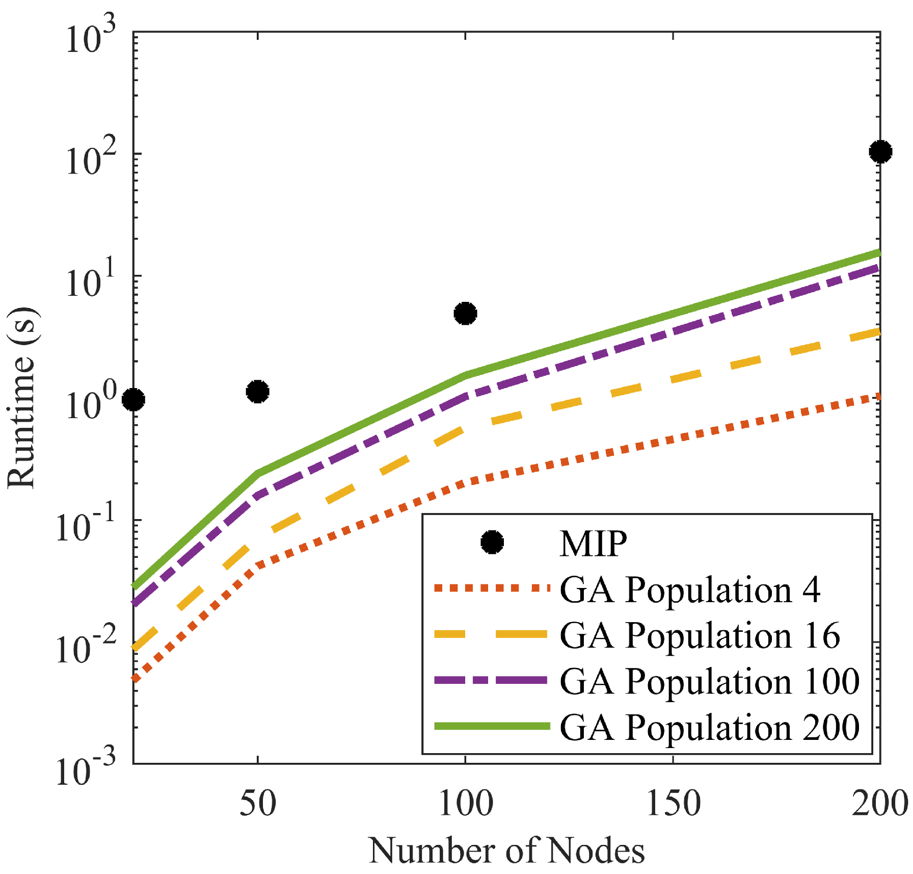
The question then arises, how close to the optimal solution is “good enough” for APS? Such a parameter could be tuned depending on real life use of APS; this analysis assumes that a GA solution with an objective function value within
of the optimal, MIP solution would be sufficient for APS. With this assumption, a test was done to compare the computation time of GA and MIP. A set of random waypoints was generated within a 10 × 100 m
2 rectangle, simulating a random row of some crop. The number of waypoints or nodes was set, and the optimal path was found with MIP. Then, four different GA configurations with varying population sizes were run to reach within
of the solution found by MIP.
Figure 6 shows the results.
Clearly, GA reaches a sufficient solution much faster than MIP converges to the optimal path. In fact, the most efficient GA configuration converges two orders of magnitude faster than MIP. The slowest GA configuration is generally one order of magnitude faster than MIP. It is also notable from
Figure 6 that smaller GA population sizes provide faster convergence. The minimum possible population size is four due to the structure of the algorithm. Furthermore, it is important to realize that the GA results of
Figure 6 had the luxury of the known optimal path. This allowed the algorithm to be terminated upon reaching the specified accuracy relative to the optimal path. If the APS is running live, it will not know the optimal path, and thus could not terminate upon reaching the desired convergence.
Fortunately, there is a reliable relationship between the required GA iterations, number of nodes, and GA runtime. A series of tests were conducted, generating random simulated crop rows as discussed previously with a range of number of nodes ranging from four to 150. The MIP solution was found, and then GA with population size four was run four different times, terminating upon reaching
of the MIP solution. Note that every new use of the GA generates a new, random initial population. Thus, each run of the GA is unique. A curve fit of this data yields that the required number of iterations
is a simple function of the number of nodes
as shown below:
In general, it is best to buffer this slightly, as Equation (
7) is a simple curve fit. Adding 10–15% to
will ensure the desired accuracy is attained with minimal runtime.
Figure 7 summarizes these results. With this relationship in hand, the GA algorithm is ready for use in APS. It has been shown that the GA is far more practical for meeting the specific needs of APS, as the vast speedup in computation time comes at the cost of a relatively small sacrifice in solution optimality. This is preferred for APS to ensure all the computational tasks required for the pollination mission can be successfully completed onboard. It is worth mentioning that constraints such as the endurance of the drone should be considered and tailored path planning algorithms need to be developed in the future to facilitate more practical solutions.
5. Flight Control
APS flight control seeks to solve the QFCP. Specifically, the six degree-of-freedom (6-DoF) QFCP seeks to control the quadrotor’s position in terms of Cartesian positions,
x,
y,
z, and orientations based on Euler angles,
,
,
. This paper makes use of the general formulation proposed by Lia et al. [
33], which requires the following state and control variables:
where the control variables,
, are a linear transformation of the forces from each individual motor,
:
In the simplest sense, the dynamics of this system can be stated as
at some time
. For the 6-DoF problem, ignoring wind or drag, this function would be defined as:
This can be equivalently expressed in the state-space form as follows:
where
This can be further separated as:
where
with
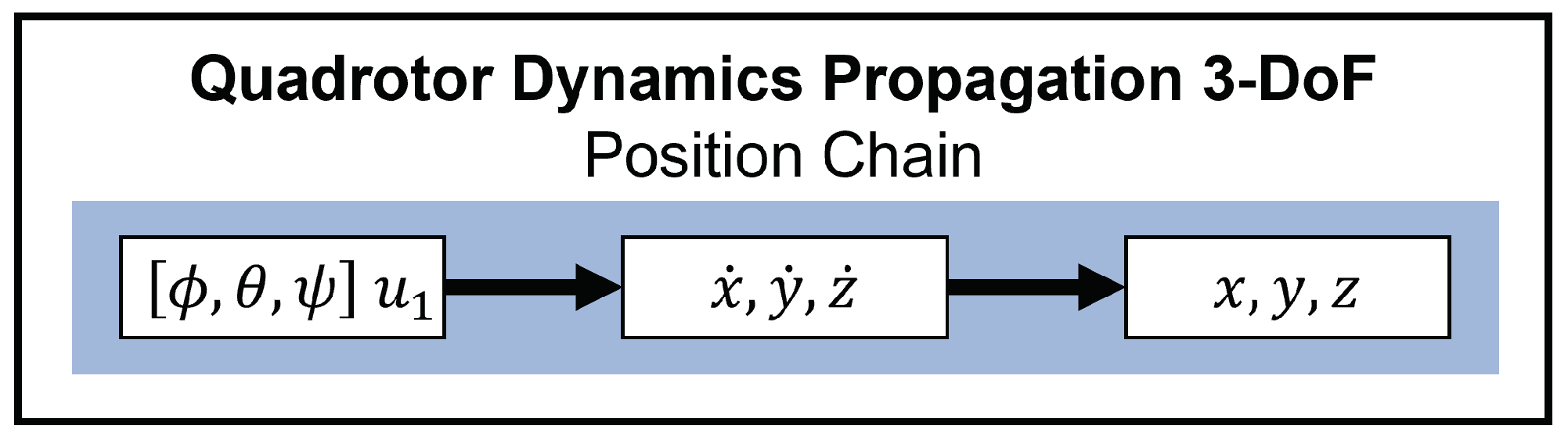
Figure 8 provides a map of how these variables are related through the dynamics. Notice the distinction between the position chain and orientation chain and how they are coupled. In
Figure 8, it can be seen that
,
,
affect
,
,
, which affect
,
,
. This is the orientation chain. The orientation chain feeds into the position chain as
and
,
,
drive velocity, which drives position,
x,
y,
z. Maintaining the coupling of these two chains is essential to maintaining the physics of any modeling of the real world based upon this formulation.
5.1. Problem Statement
The QFCP in its simplest sense seeks to control a quadrotor such that it will fly from one position to another, for example, from A to B. To apply optimization to solve this problem, the state and control variables are required to be physically feasible and meet the flight requirements. An optimization approach also allows the user to find a solution maximizing or minimizing some objective aside from the basic movement from A to B. This could be obvious objectives such as minimizing control effort or flight time, but the optimization approach allows for great flexibility in defining an objective. The proposed QFCP approach seeks to minimize control effort. Thus in the most general sense, the problem is formulated as follows.
Note that this problem formulation ignores collision avoidance.
To numerically solve this problem, we choose to discretize the problem using some integration rule. Suppose that the time interval
is uniformly discretized into
points,
. Thus, there are
N discrete time steps of size
. This paper applies a trapezoidal integration across this mesh, but a Runge–Kutta or Euler integration would also be suitable. Trapezoidal integration takes the following form.
In this way, the original dynamics are expressed as equality constraints, and the continuous-time Problem 1 is transformed into a numerical optimization problem. What makes this problem impractical in this general sense is that Equation (
13), the dynamics, are highly nonlinear, nonconvex. While a solution can be found to such problems, it is well known that general nonlinear optimization is too slow or unstable for real time applications. This necessitates the convexification of the problem to facilitate the application of more efficient optimization algorithms. Specifically, if the problem can be reformulated into a convex optimization problem, highly efficient algorithms such as interior-point methods can be applied which will enable real time flight control based on this formulation.
5.2. Convex Dynamics
Now, an approach to the convexification of the nonlinear dynamics of the quadrotor system will be presented. This approach relies on successive linearization. It begins by breaking the dynamics in Equation (
13) down further as
with
being the linear portion of the matrix
mentioned in Equation (
13) and
containing only the nonlinear elements of the dynamics. The difference between
and
is that
is all zeros in the first column, i.e., it does not contain the nonlinear terms that
does.
Equation (
16) is still nonconvex. To convexify it, a dynamic linearization is employed. Equation (
17) shows the dynamic linearization of
, which contains the nonconvexity of the formulation.
where
and
are an initial guess or previous iteration solution. Note that the fidelity of the linearization declines as
and
become larger. Clearly, when
and
, the linearization is exact. This fact necessitates that a trust region be employed, thus limiting the magnitude of change from the initial guess or previous iteration. The trust-region constraints take the form of
and
.
Combining Equations (
16) and (
17) yields the following:
The nonlinear portion,
, is defined as:
The partial derivative of
with respect to the state vector
X and controls
U are defined as follows:
This successive linearization maintains the coupling of the position and orientation chains. One strength of the convexified dynamics is that the linearization is only applied to the function . Thus, only the nonlinear terms are affected by the linearization. In fact, only the variables and , , and are affected by the linearization. This means that while and , the values from an initial guess or previous iteration, are necessary for the formulation to work, the only variables that must be included in this initial guess or previous iteration reference are and , , and . It is also important to note that other variables are unaffected by linearization and thus a trust region is not necessary for them. A new, linearized convex problem is obtained as follows.
Note that
and
could be uniform vectors or each variable could be given a different trust region size based on how it is affected by the linearization. In fact, one only necessarily requires that,
for
and scalar
.
Problem 2 provides a convexified 6-DoF QFCP, which requires an initial guess or reference point. Thus, the next step to solve the QFCP will be to find means of providing a sufficient guess. One possible approach could be to implement an SCP scheme, as the linearized dynamics are well suited for such an approach. It was found that solving a simplified, convex, three degree-of-freedom (3-DoF) problem that only accounts for the position chain and using that solution as the initial guess for Problem 2 works quite well. The following subsection develops this 3-DoF problem.
5.3. Three Degree-of-Freedom Problem
The 3-DoF QFCP only addresses the position chain of the larger 6-DoF problem. Again, the only variables necessary for an initial guess are
and
,
, and
, so the primary goal of the 3-DoF problem is to extract these variables. The simplified problem consists of the following variables and dynamics. Notice that
,
, and
are treated as controls in this formulation.
This new formulation yields the following optimal control problem.
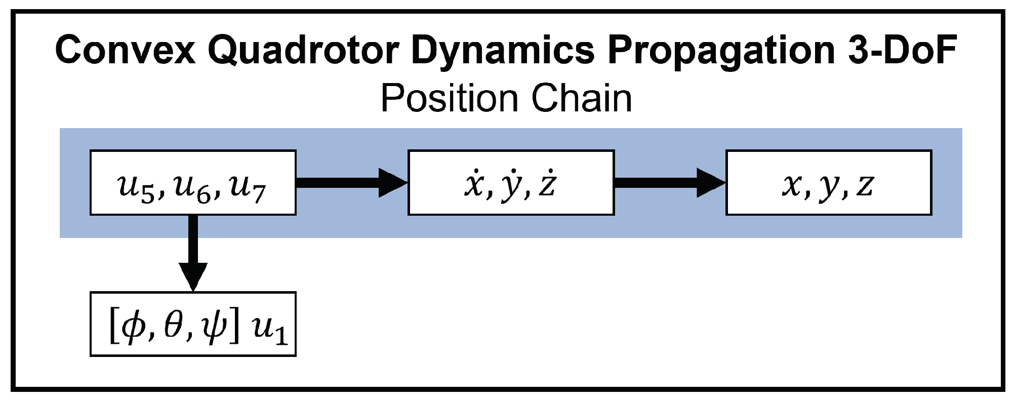
The variables in this problem are related as in
Figure 9.
However, Problem 3 is still nonconvex because of the highly nonlinear dynamics. A change of variables can be employed to convexify the problem. Specifically, we define three new variables
,
, and
as follows:
These variables are related and dependent as in Equation (
32) due to trigonometric properties:
Note that , , and are the projections of onto the x, y, and z axes. Reformulating Problem 3 with these relations yields:
Problem 4. whereand the state and control vectors This problem will find the minimum control effort of the QFCP in terms of variables
,
, and
. From these, the orientations
,
, and
and control
can be found using Equations (
29)–(
32).
Figure 10 demonstrates the propagation of the variables in this problem, which provides an initial guess that will be used in the full, 6-DoF problem using the dynamics expressed in Equation (
18).
5.4. Two-Convex-Problem-Approach Discussion
The previous two subsections defined a two-convex-problem approach to the QFCP. Problem 4, the convexified 3-DoF problem is solved, and the solution to this problem serves as the initial guess to Problem 2, a 6-DoF problem with linearized dynamics. The solution to this problem will be a valid flight trajectory with all four controls successfully solved. Even with small
, there will be some deviation from the true dynamics. This can lead to some suboptimal solution behavior, as the linearized system is finding a solution minimizing
, and it will necessarily find that solution on the edge of the region that is the trusted region expressed in Equations (
23) and (
24) due to the nature of linear functions.
Problem 2 seeks to find the minimum control effort trajectory of the QFCP. Problem 2 takes the solution, or part of the solution, of Problem 4 as an initial guess and only allows for a certain deviation from that initial guess. In fact, in many cases, Problem 4 will have already found the minimum control effort trajectory of the QFCP, and Problem 2 will, in most cases, choose a solution minimizing control effort, but that will likely not be entirely accurate to the original system dynamics. An alternative is to assume that the solution to Problem 4 is the correct minimum control effort trajectory of the QFCP and solve Problem 2, but now minimizing deviation from that optimal trajectory. In a sense, this approach solves the position chain with Problem 4, and then updates the orientation chain respectively with the 6-DoF problem. Thus, a new problem can be formulated as follows.
Note that the first objective function formulation only minimizes the deviation of the variables affected by linearization while the second objective function formulation allows more flexibility to minimize deviation from the other values of the initial guess.
Problem 5 will provide a physically feasible solution that is as close to the simplified 3-DoF problem (Problem 4) as possible. Thus, two possible convex optimization approaches have been proposed. Approach 1 is to solve Problem 4 to provide an initial guess to the convexified Problem 2. Approach 2 is to solve Problem 4 to find an approximate optimal solution to the position chain of Problem 1, and then update the orientation chain variables to match this trajectory using Problem 5.
Approach 1 is more intuitive. It is merely a scheme to develop a feasible initial guess to the convexified Problem 2, and both problems are directly related to Problem 1. It is possible that this will provide an exact solution to Problem 1, but it is expected that this procedure will produce an approximate solution, as the linearization will introduce a small degree of inaccuracy in the physical dynamics. For small , this deviation from reality will be negligible.
Approach 2 is less intuitive. The 3-DoF Problem 4 is solved, and its solution is assumed to be the correct solution to the position chain of the original minimum control effort QFCP (Problem 1). The orientation chain is then updated while minimizing deviation from the true, physical dynamics. The strength of this approach over Approach 1 is that it will produce solutions that better represent the original dynamics. For this reason, Approach 2 is chosen as the preferred approach in this paper. Both approaches will produce an approximate solution to the original QFCP (Problem 1) but Approach 2 will produce a physically feasible approximate solution.
5.5. Numerical Results
To verify the solutions found through the presented convex optimization approach, GPOPS-II [
34] was applied to solve Problem 1 for comparison. GPOPS was developed at the University of Florida as commercial general purpose nonlinear optimal control software. It is a MATLAB compatible tool that can solve a wide range of nonlinear optimal control problems, including such problems related to quadrotors. GPOPS relies on an adaptive mesh refinement technique and uses IPOPT or SNOPT to solve the resulting numerical optimization problems. However, the convergence and computational cost of GPOPS cannot be predicted when solving large-scale, highly nonconvex problems. In contrast, the proposed convex optimization approach leads to two convex programs with fixed step sizes and controllable problem scales that can be efficiently solved using convex solvers with guarantees on convergence given that the problems are feasible and solutions exist. However, the methods are still comparable in terms of objective function value and solution behavior.
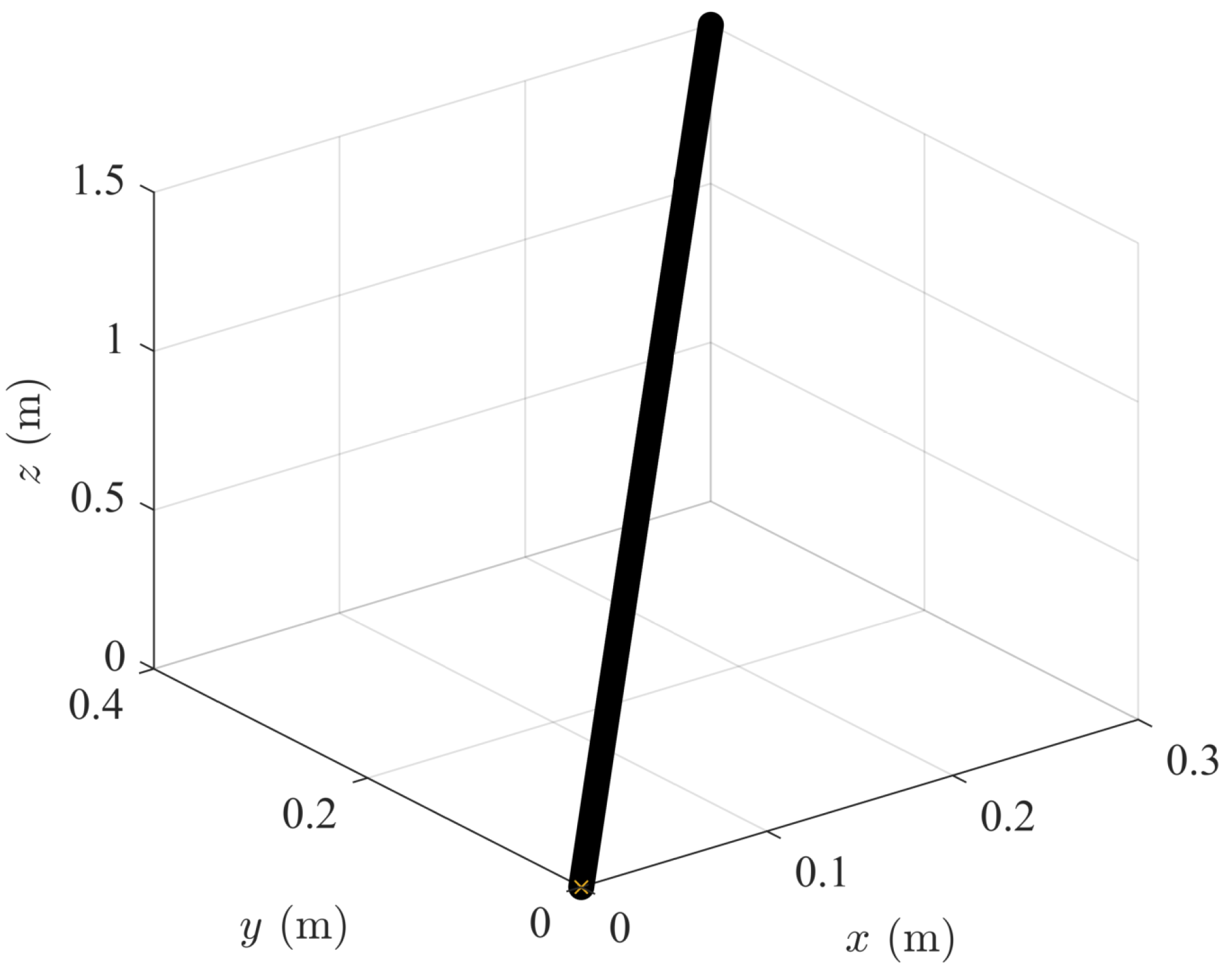
The following will demonstrate Approach 2 in a short flight from a position
to the origin given two seconds to reach the final position with 10 nodes and again with 400 nodes. The demonstration assumes a drone with the same parameters as found in Lai et al. [
33]. Thus
kg·m
2 and
kg·m
2. The quadrotor has a mass of
kg and gravity is
m/s
2. The maximum thrust from each motor is 10 N, so
N and
N. The results are shown in
Figure 11,
Figure 12,
Figure 13,
Figure 14,
Figure 15,
Figure 16,
Figure 17,
Figure 18,
Figure 19,
Figure 20,
Figure 21,
Figure 22,
Figure 23,
Figure 24,
Figure 25,
Figure 26,
Figure 27 and
Figure 28.
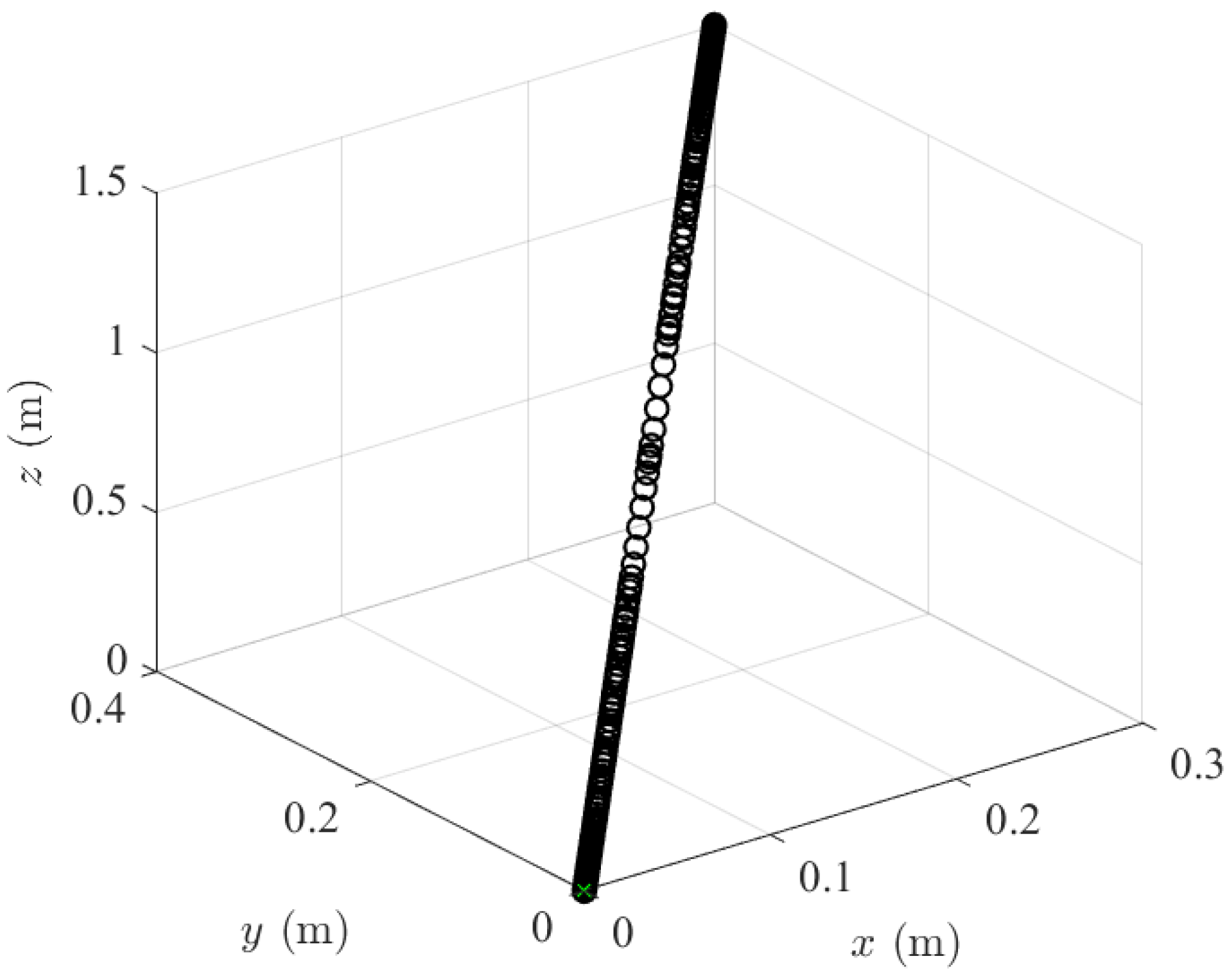
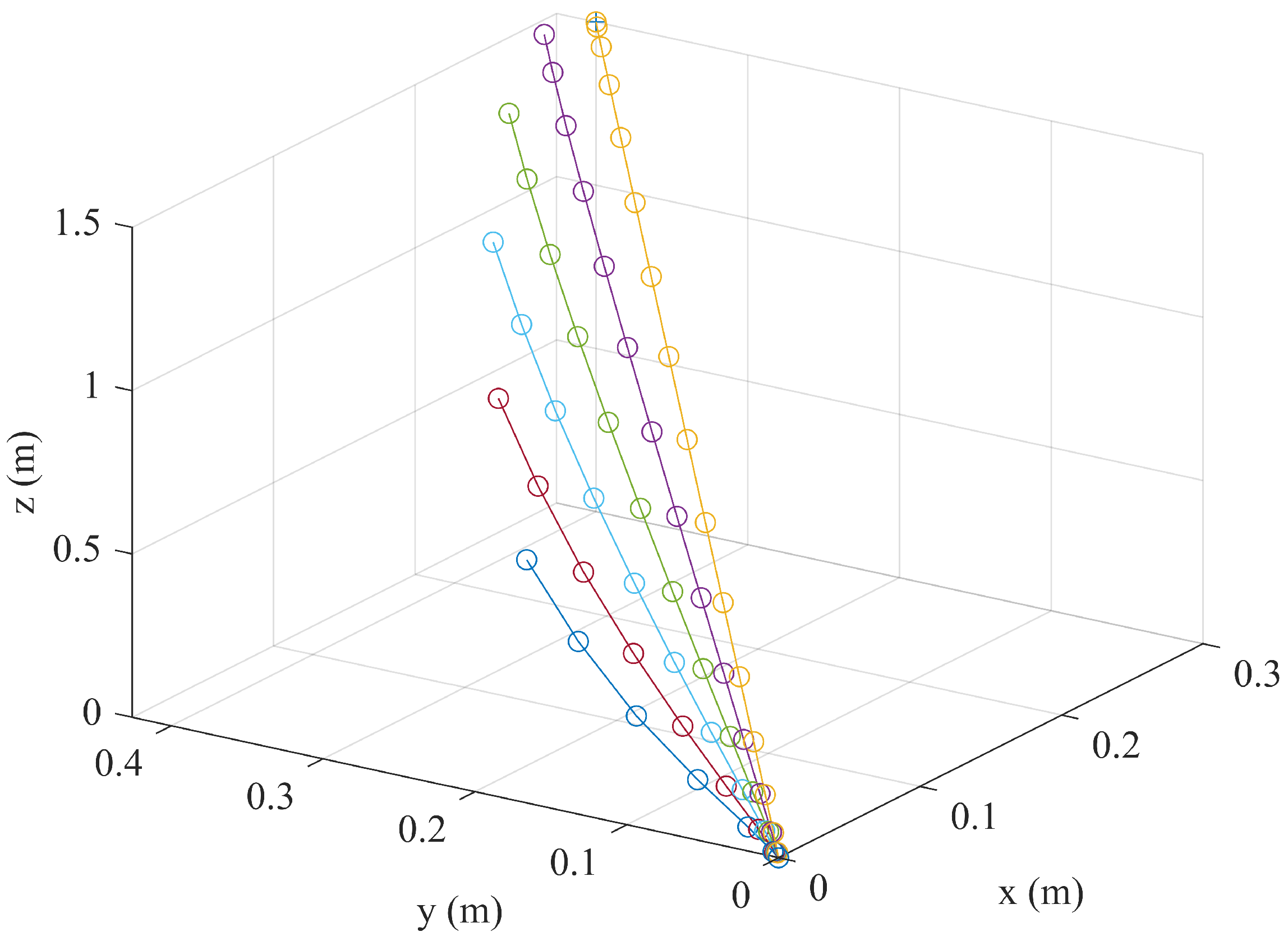
Figure 11,
Figure 12 and
Figure 13 show the 3-D trajectories of the three simulated cases (i.e., 10-node convex, 400-node convex, and GPOPS). The resulting trajectories are characterized as being almost a straight line from start to finish and quickly accelerating and decelerating. This is similar to a “bang-off-bang” trajectory. GPOPS provides similar solutions to the two convex approach solutions, though the effect of the adaptive mesh is clear. The GPOPS solution contains 453 nodes, as opposed to 10 and 400 nodes that were used for the convex approach. As a result, one observes that the solutions with more nodes appear continuous relative to the convex approach with 10 nodes. Similarly, it is observed that the convex approach solution with 400 nodes is similar to the GPOPS solution in almost every regard. Thus, the 400 node solution shows that the proposed convex approach converges to practically the same solution as an accepted, but more computationally efficient, method of control than GPOPS.
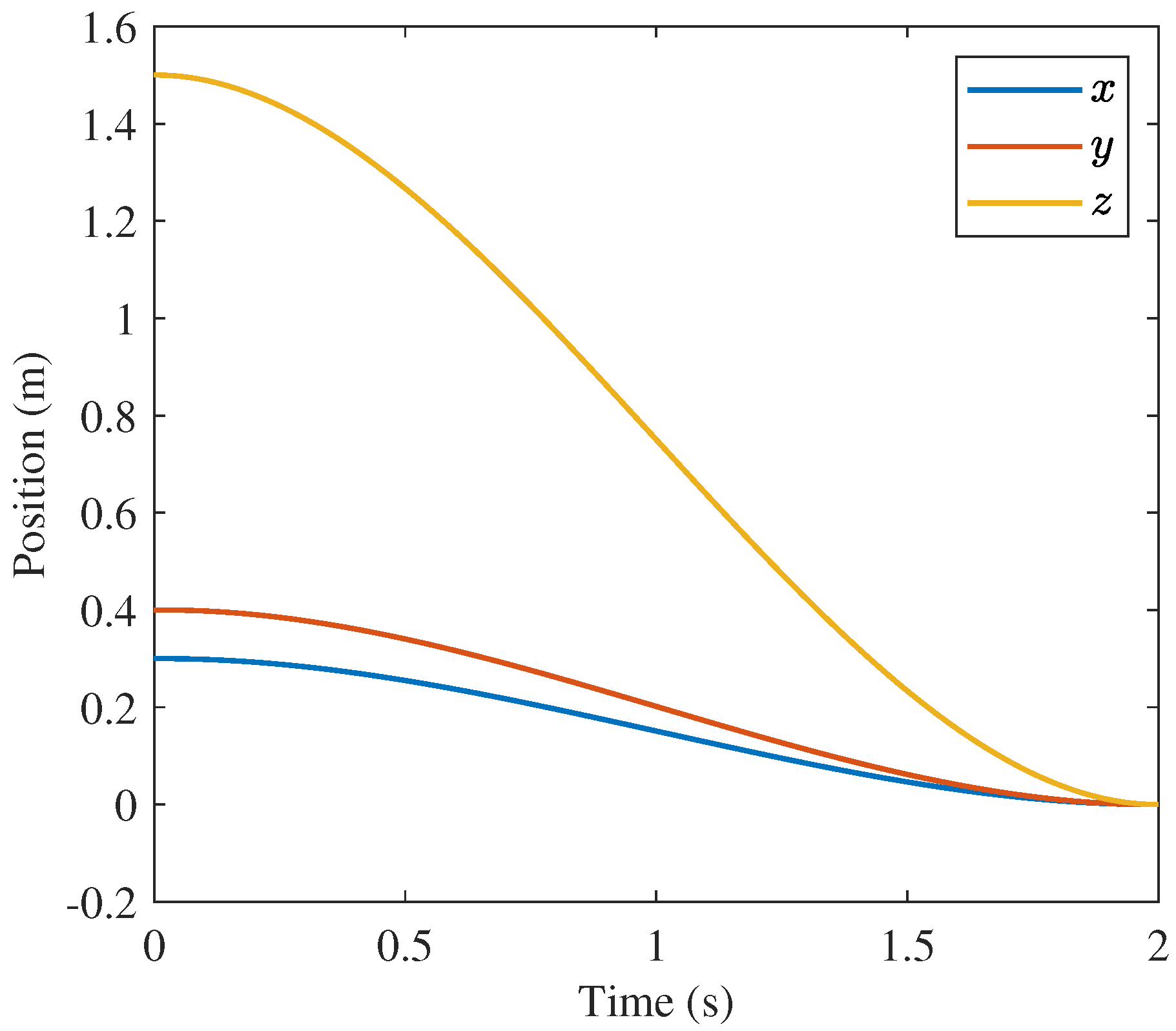
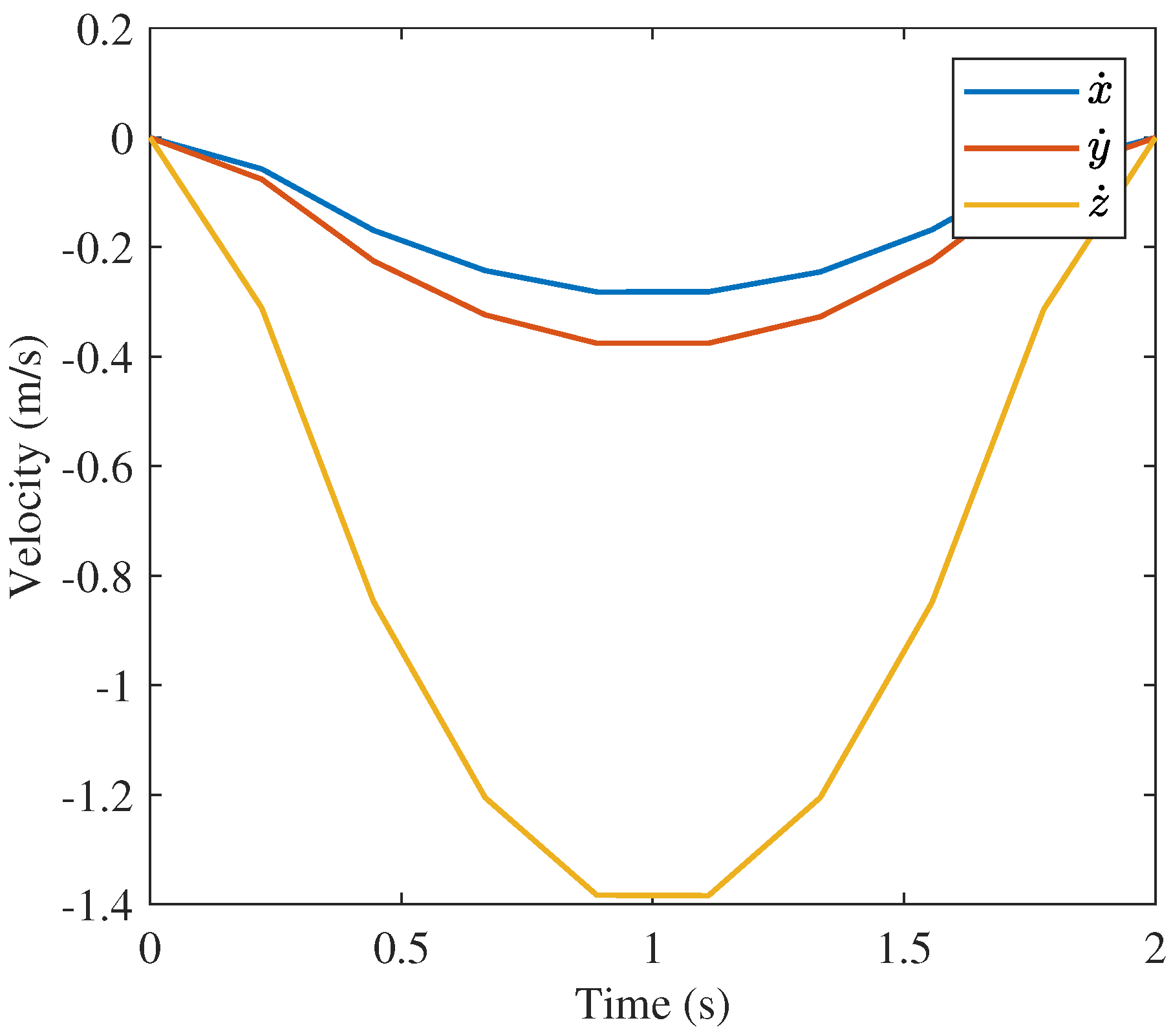
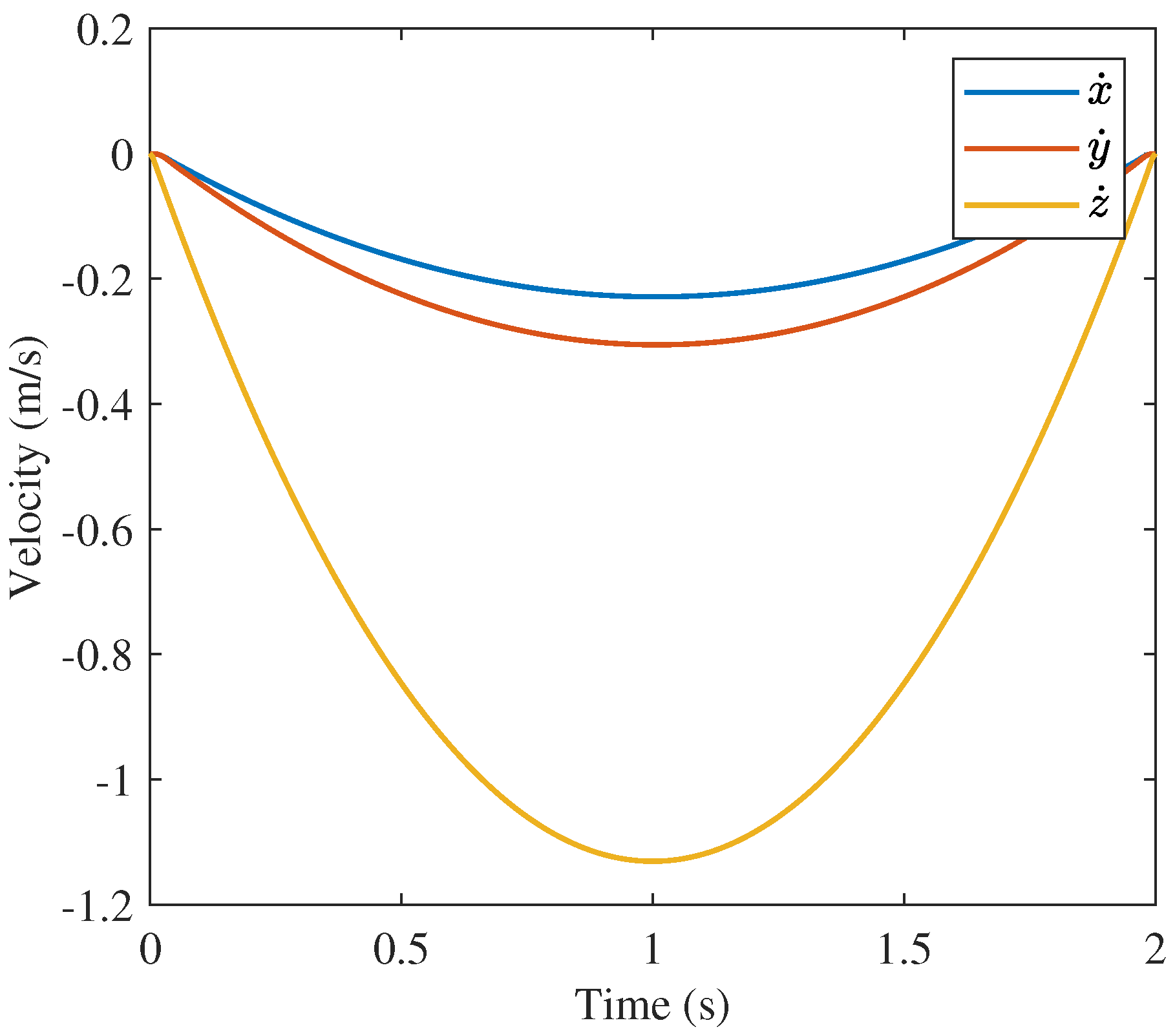
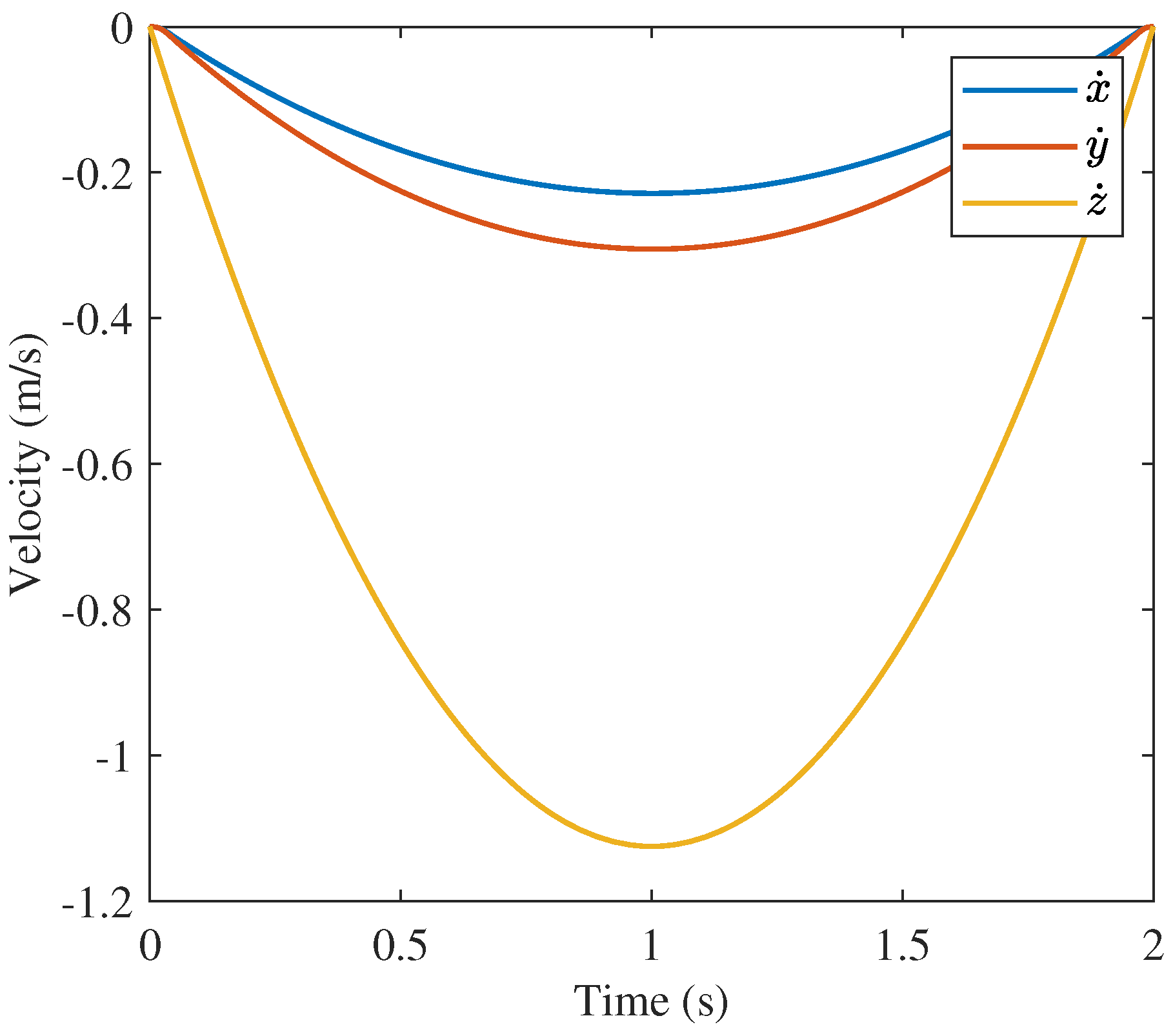
Though GPOPS and the 400 node convex solution are similar, the 10 node convex approach solution is less obviously similar to the GPOPS solution. The position and velocity profiles are very similar as shown in
Figure 17,
Figure 18 and
Figure 19 and
Figure 23,
Figure 24 and
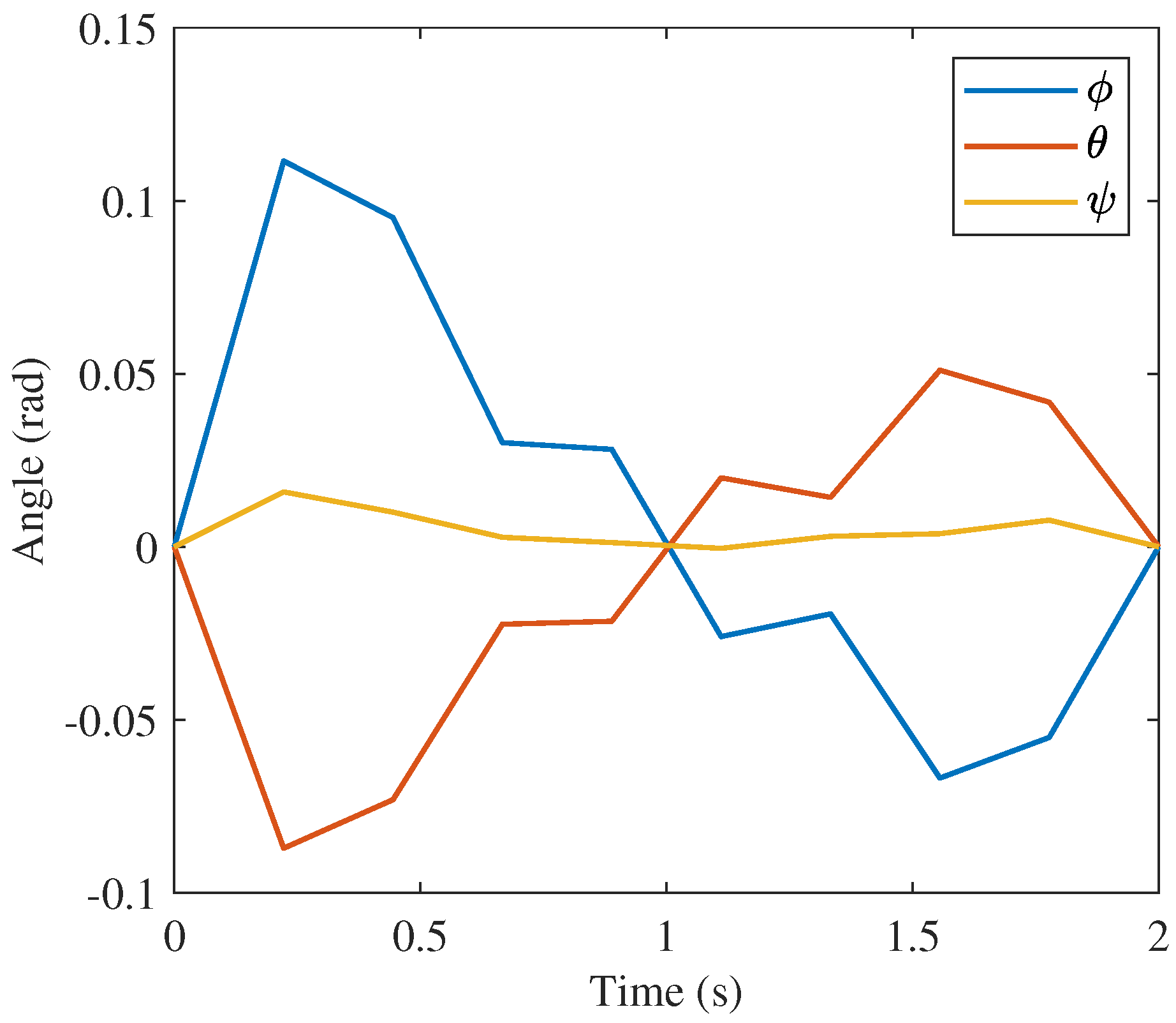
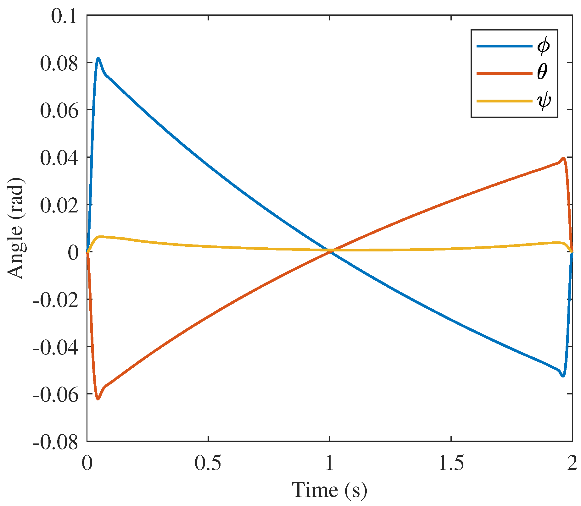
Figure 25, respectively. Similarities are also present in the orientation profiles in
Figure 20,
Figure 21 and
Figure 22 with
and
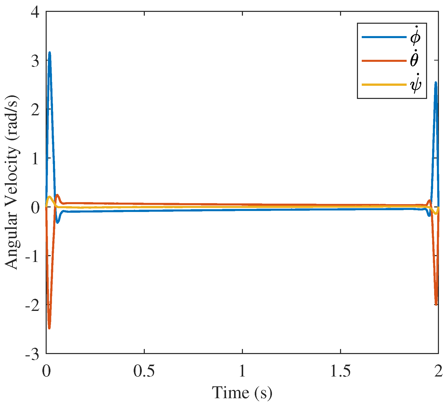
rising and dropping to similar magnitudes in the solution from GPOPS and that from the proposed approach with 10 nodes. The angular velocity profiles in
Figure 26,
Figure 27 and
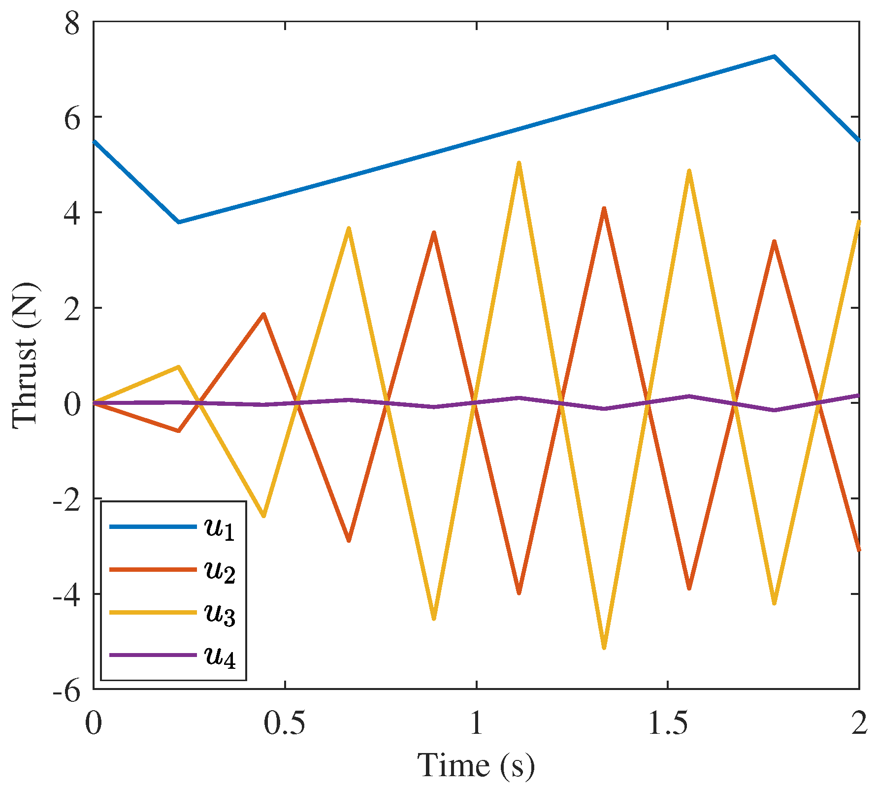
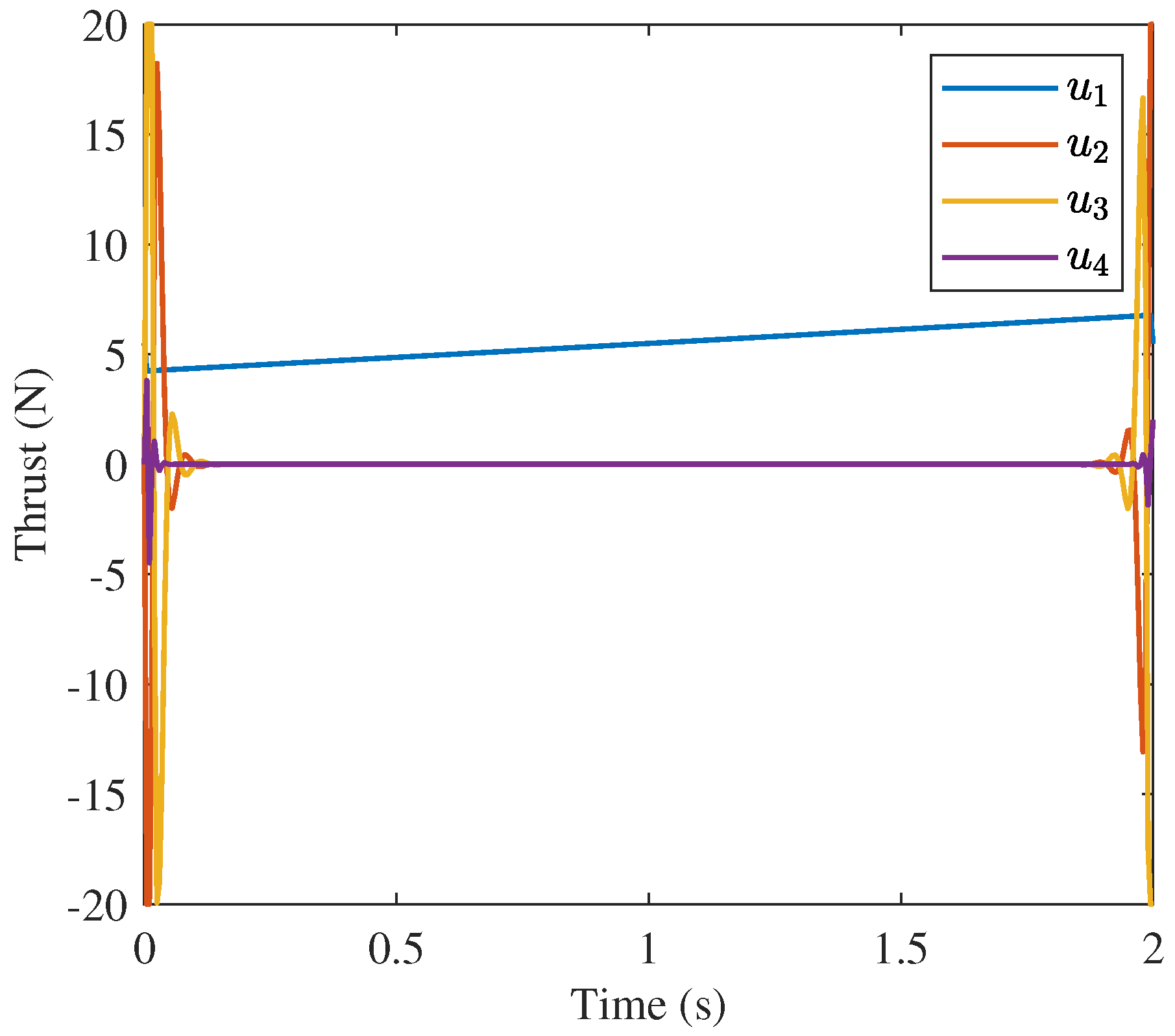
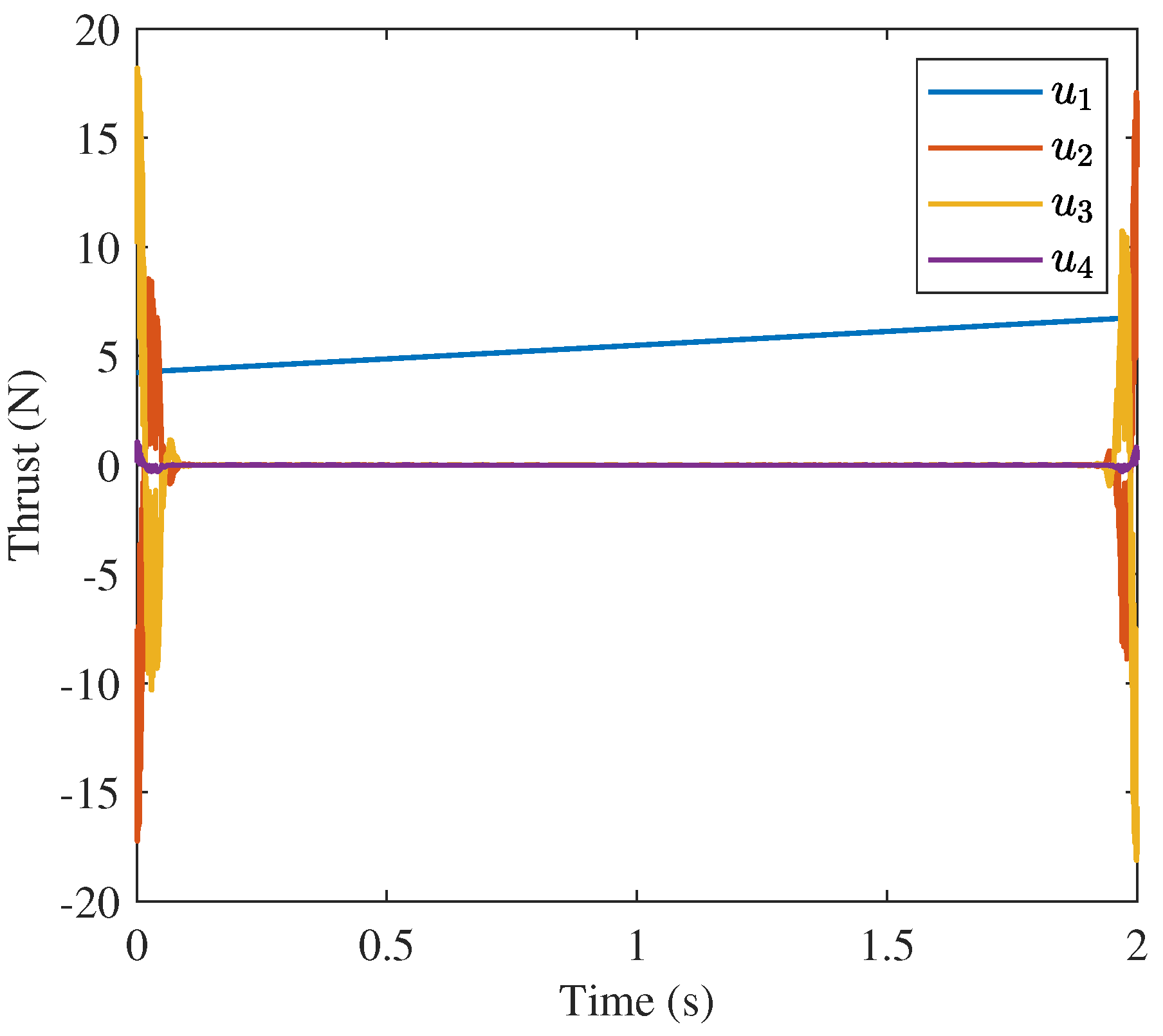
Figure 28 are less obviously similar to the GPOPS solution. Similarly, the control profile for the 10 node convex solution shown in
Figure 14 has a similar
solution to the GPOPS and 400 node solutions as shown in
Figure 15 and
Figure 16, respectively, but controls
are very different. The 10 node solution for
is oscillatory while to other two solutions are strongly characteristics of the “bang-off-bang” trajectory. The strong difference between the behavior of the 10 node solution and the other two solutions is a product of the number of nodes and the inner workings of the approaches such as the discretization method (trapezoidal rule vs. collocation), optimization algorithm (nonlinear programming vs. convex optimization), etc.
All three solutions have similar objective function values. The convex approach with 10 nodes provides a minimal control effort objective function value of N2s. GPOPS and the 400 node solutions have objective values of N2s and N2s respectively. The small deviations among these solutions is a result of integration over different number of nodes and different step sizes.
The strength of the proposed convex approach is its computation time. The convex approach with 10 nodes reached this solution in 0.65 s. GPOPS simultaneously took 9.72 s. This is a speedup of 15x. The convex approach with 400 nodes took 21.015 s. While this is more than twice as long as GPOPS, the convex approach will never be run with so many nodes in practice. As previously stated, flight controllers can only send and receive commands with some maximum frequency, making large numbers of nodes impractical for live flight. The 400 node test is only presented to show the nearly exact result as GPOPS. These simulations were performed using MATLAB on a Lenovo IdeaPad Flex with an Intel CORE i5 8th Gen processor.
The speed and parameter control that the convex approach provides make it well suited for online applications. The step size, number of nodes, and desired state can be specified, and a solution taking into account the highly nonlinear dynamics of the system can be generated in a short time. For APS, this reduces the cost of flight control on the processor, thus allowing more computation power for the rest of the system.
One very important consideration in the use of the proposed convex approach is the number of nodes. In many missions, a smaller number of nodes (e.g., 5 to 20) will be more practical, and it has been shown that with many nodes, the convex approach will provide a solution that is quite similar to GPOPS. Due to the structure of the two convex optimization problems, the proposed approach will always fail if 6 or 12 nodes are used. If 6 nodes are used, the 3-DoF problem will be infeasible, and thus the 6-DoF problem will fail without a feasible initial guess. Similarly, if 12 nodes are used, the 6-DoF problem will be infeasible. This issue can be easily overcome by simply using a different number of nodes, as, if the problem is feasible, 5, 7, 11, and 13 nodes will provide feasible solutions. In the next section, the convex approach will be used within an MPC framework. In doing this, there were inevitably scenarios when the framework would naturally use 6 or 12 nodes. In these situations, the number of time steps of controls applied was momentarily modified to skip over the infeasible numbers of nodes.
The method also requires that at least five nodes be used in most cases. This is simply due to the fact that the first and last nodes are usually fixed to the start and end position. Thus if only two nodes are used, the optimization problem will obviously be infeasible. If three or four nodes are used, there generally is not enough flexibility in the one or two free nodes to provide a feasible solution. The effects of the number of nodes on the feasibility of the resulting convex problems and the performance of the developed convex optimization approach need to be further investigated in the future.
In addition, the convex approach does not currently incorporate collision avoidance. Collision avoidance constraints are nonconvex and thus create new difficulties to convexify the problem. The authors define two scenarios for collision avoidance, sparse environment collision avoidance and local collision avoidance. Sparse environment collision avoidance refers to avoiding obstacles in a generally open space, like flying through a building or avoiding large obstacles. This form of collision avoidance can be easily incorporated into path planning. This can be done by defining convex flight corridors or convex ducts during path planning that can be used as convex constraints in the resulting flight control problems. For example, if the quadrotor needs to fly through a doorway, a convex shape can be easily defined to constrain the flight of the quadrotor to fly safely through the door with the proposed convex approach. It is noted that while this can be easily done from a flight control and path planning perspective, it creates new machine vision tasks that must be addressed to provide the necessary information for this procedure.
Local collision avoidance refers to scenarios where convex flight corridors cannot be easily defined and is more difficult to incorporate, as it will need to be directly integrated into the flight control algorithm. For example, APS will require a drone flying around the plants that it is pollinating to reach flowers on the other side. In such cases, it will not be possible to define a convex shape for the drone to fly within. Thus, the nonconvex collision avoidance constraints will need to be incorporated into the flight controller. These constraints are not incorporated within the convex approach proposed in this paper; however, similar approaches have been successfully implemented by other researchers. One approach that is promising is the use of SCP by [
28] to gradually incorporate the collision avoidance constraints into the optimization problem. It is our plan to extend our proposed APS and the developed convex approach to address pollination problems under collision avoidance constraints in the future.
The most comparable research to the proposed approach is Mueller and D’Andrea’s work [
26]. The proposed approach solves a 6-DoF QFCP, which has many solution methods, but there are few examples of the problem being convexified and solved as in this paper. Mueller and D’Andrea were able to convexify the problem by reformulating the dynamics in terms of jerk and thus decoupling the axes and convexifying the problem. This contrasts with our proposed approach which solves the QFCP more directly in that the original problem formulation is maintained, though an initial guess is found using a 3-DoF formulation. These different convexifications will provide different results. Mueller and D’Andrea’s jerk reformulation will result in different solution spaces than the use of the 3-DoF initial guess proposed in this paper. Much further research is necessary to determine the performance differences of these two approaches to convexification, though it is certain that the reliability and speed of the convexified problem is inherent to both solution methods.
6. Model Predictive Control
In order to apply the presented path planning and flight control algorithms for real-world pollination missions, we implement these algorithms online within a receding-horizon framework. MPC is the chosen framework for the task and it provides great flexibility for APS. MPC is a closed-loop control framework that incorporates a moving time horizon. This approach has a few benefits. By solving the control problem over a finite period or horizon, a smaller problem is solved, reducing computation time. Simultaneously, by resolving the control problem at intervals, the system adjusts for deviations from the previously solved problem. This embeds corrections to the system directly into the framework.
For APS, path planning and flight control must be coupled together through MPC for mission execution. MPC can also be applied to path planning and flight control separately. In this section, MPC applied to path planning and flight control individually will be presented first and then the APS implementation of them will be discussed.
6.1. Path Planning MPC
A simulation of the GA path planning algorithm within an MPC framework has been performed to demonstrate the benefits of MPC. A set of random waypoints was generated within a
m
2 rectangle, simulating a random row of some crop. 100 waypoints were generated for the test. MPC uses a receding time horizon and a distance horizon for computational efficiency. In the context of APS, that means that MPC will only predict and optimize the sequence of flowers within some distance of the quadrotor and for some short time. In the small rectangle that was generated for this demonstration, a 60 s time horizon and 20 m distance horizon were used.
Figure 29 shows four distinct instants during the simulation.
In
Figure 29, the blue circles represent the waypoints or flowers. The red line represents the optimal path found through GA. There is a large red dot that represents where the drone is currently located. This is usually the left most point. The top frame of
Figure 29 is the initiation of the simulation. Each successive frame is a snapshot of the MPC path plan at a given time. Notice that the path ignores all waypoints 20 m beyond the current location and any waypoints it has already visited. The drone is assumed to just continue to the end of the row when it reaches this point. By only dealing with the waypoints that are within a short distance of the drone, MPC greatly reduces computation time at each path update.
Calling back to the relative performance of GA and MIP, performing this simulation four times using both MIP and GA provided more insight into the computational time savings of GA. Over the four simulations, GA averaged 0.7621 s of path planning computation while MIP averaged 6.741 s. MIP took, on average, almost nine times longer to compute during the simulation. MIP also had much more variation in computation time. GA computation time had a standard deviation of 0.035 s over the four tests. MIP’s standard deviation was 7.327 s. This variation is 4.6% of average computation time of GA as opposed to 108.7% of computation time for MIP. The computation cost savings and consistency provided by GA came at the cost of an 8.13% increase in total distance travelled on average over the four tests. If this was a live flight test, clearly GA would be much preferred due to the huge computational savings and reliability with only a relatively small increase in total distance travelled.
6.2. Flight Control MPC
The implementation of MPC for flight control is slightly different. For this implementation, the goal is to generate controls to maneuver the quadrotor to its destination. This is done in a shrinking horizon sense. Shrinking horizon refers to generating a series of controls over some number of time steps, n, implementing the first few, m, of these controls, and then generating a new series of controls over the remaining timesteps. This process is repeated until the target is reached or perhaps there are just a few timesteps remaining and some procedure is initiated.
Figure 30 demonstrates this framework using the same flight scenario as described in the flight control section, but now with a small wind blowing in the positive
y direction. The quadrotor begins at position
and generates a series of controls to fly to the origin. This is the tallest trajectory in the figure. The first two of these controls are implemented. The wind is not incorporated into the optimization model, so these commands result in a position that is further in the
y direction than anticipated. A new command sequence is generated to adjust, and the process is repeated five times.
The corrective behavior of the MPC framework is clear from this demonstration. The controls adjust to the fact that the quadrotor is not in the previously predicted position. These embedded adjustments increase the likelihood of a successful mission under inevitable uncertainties and disturbances in real-world implementation.
6.3. APS MPC
Finally, the flight control and path planning algorithms were coupled together within MPC. This implementation simply used the path planning MPC from
Section 6.1 and the flight control MPC from
Section 6.2 in tandem. This simply means that the path planning MPC generates a list of destinations that the flight control then flies to. In truth, this is actually two separate implementations of MPC; one of these implementations operates within the other.
Figure 31 shows how these two MPC implementations interlace.
Figure 31 demonstrates how the flight controller, in red, uses an independent MPC implementation within the larger, coupled MPC, in blue. Both MPC implementations receive a goal and current state as input and provide a control sequence as their output. The difference between them is that the coupled MPC goal input is to reach each waypoint or flower. The flight control MPC goal is to reach the next waypoint or flower in the list, the desired state or location. The flight control MPC will update at a much faster frequency than the coupled MPC, i.e., it will have a much smaller time horizon. For example, the flight control MPC may update the control sequence every second, while the coupled MPC may only update every minute, as the flight controller should be given time to reach the desired location, the next waypoint in the optimal path.
Figure 32,
Figure 33 and
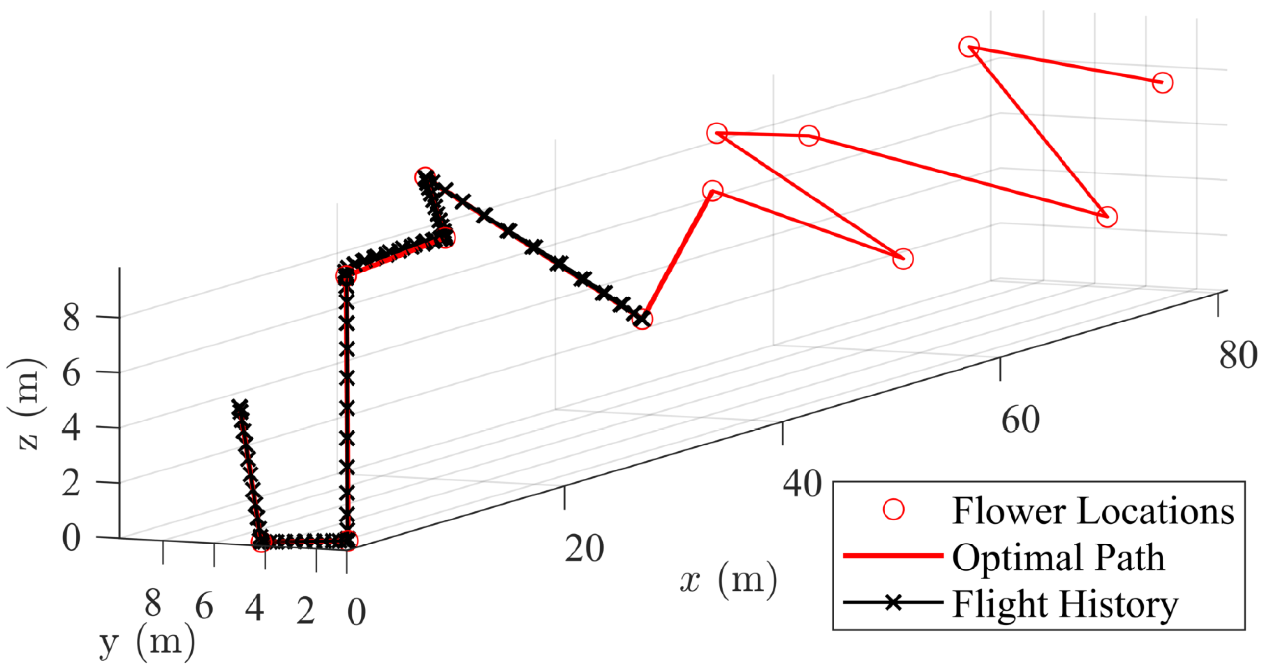
Figure 34 show three snapshots of the APS MPC in action.
Figure 32 shows the start of the simulation. At this point, the quadrotor has not moved yet, but the path planning module has assessed the flower locations (red circles) within its horizon. A path has been defined and passed on to the flight control module. This path is visualized with the red line connecting some of the dots.
Figure 33 shows a snapshot of after the algorithm has run for a few seconds. The flight path of the quadrotor is show in a series of points, and it is seen that the quadrotor has reached three of the flower locations. More flower locations have come into the horizon of the path planning module and have thus been added to the path.
Figure 34 shows a final snapshot of after the algorithm has run for another few seconds. It is seen that more of the flowers have been pollinated and more locations added to the path.
MPC is a flexible framework that can allow for many different implementations. In this implementation, the flight controller was given two seconds for each flower-to-flower flight with a time step of 0.2 s and a time horizon of 0.4 s, meaning that two time steps of control output were implemented before regenerating controls. At the start and every time a flower was reached, the path planning algorithm was re-run with a horizon of 0.5 m.
7. Conclusions
In this paper, we propose a drone-enabled autonomous pollination system (APS) consisting of five primary modules: environment sensing, flower perception, path planning, flight control, and pollination mechanisms. Highly efficient algorithms have been developed and demonstrated for the flower perception, path planning, and flight control modules. First, flower perception based on orthoimages of the crop fields was briefly discussed. R-CNN was used to detect flowers within orthoimages and create a map of flower locations, which was passed on to the path planning module. Second, two solution methods, MIP and GA, were tested for APS path planning, and GA was found to be much better suited for the task. Third, a convex optimization-based flight control method was developed and numerically demonstrated. This convex approach to the QFCP minimum control effort relies on solving two convex problems. The first convex problem is a convexified 3-DoF formulation that solves the position chain of the QFCP and provides an initial guess for the second problem, which is a linearized version of the full 6-DoF QFCP. This approach was demonstrated and compared to the solution provided by GPOPS. It was observed that with a large number of nodes, the proposed approach provides a similar solution to that generated by GPOPS. The solution was found to generate a solution 15 times faster than GPOPS when solving with 10 nodes. This speedup and the control over the number of nodes in the trajectory make the convex approach highly practical for generating controls that can be used for flight control.
Furthermore, an MPC implementation of the path planning and flight control modules was demonstrated, and then simulations were performed that coupled the two modules together as they would be in an APS mission. The path planning MPC simulation further demonstrated the merits of GA over MIP. GA was 23x faster than MIP with negligible effects on total distance travelled. The flight control MPC simulation demonstrated the corrective aspects of the MPC framework, with the trajectories updating accordingly as the wind gust moved the quadrotor away from its expected location. These two MPC implementations were coupled together in a final demonstration of a true APS mission. Flower locations were generated, path planning developed an optimal sequence of these locations, and flight control successfully generated controls and trajectories to maneuver through the locations.


 ,
, 


