1. Introduction
The industrial demand for automated driving technology is increasing, and this technology has made remarkable progress in providing promising transportation to our lives [
1,
2]. However, vehicle motion planning for automated driving needs further development which considers multiple constraints in sparse information environments; in these environments, macro information is known and micro information is unknown and uncertain, especially for safe, effective, and precise motion planning. In automated driving, a real traffic environment is full of uncertainty due to information incompleteness, traffic disturbances, and other factors such as the incomplete information provided by vehicle sensors and the disturbances of obstacles, which lead to complex traffic environments that may be difficult to predict in real time [
3].
Various of traditional motion planning methods (non-data-driven methods) use heuristic algorithms [
4], sampling-based methods [
5], and rule-based methods [
6,
7] for automated driving. Although these methods perform well via solid mathematical models in terms of robustness, interpretability, and stability, they still need considerable human knowledge in advance; therefore, modeling the complex and uncertain environments using these models is difficult, and these models might not perform well under unknown and uncertain environments. However, reinforcement learning (RL) (data-driven methods) [
8,
9,
10] does not need a lot of human knowledge in advance and may perform better in unknown and uncertain environments via trial-and-error learning, which can model complex environments using data-driven methods [
11]. For example, AlphaGo shows superior performance via RL [
12] as compared to humans in the Game of Go, which is one of the most challenging games that exist; Gu et al. provided a multi-agent RL method that could teach multiple robots how to run in a multi-agent system while considering the balance between the robots’ rewards and safety, in which an agent not only needs to consider its own reward and other agents’ rewards, but also its safety and other agents’ safety in unstable environments [
9].
Indeed, agents using RL methods can learn how to automatically navigate a vehicle via exploration and exploitation [
13,
14]. Therefore, combining RL with traditional methods is significant as it can achieve better performance in uncertain environments for vehicle motion planning. However, how to combine traditional methods with RL and consider safe, effective, and precise motion planning while leveraging the advantages of these two methods and overcoming their shortcomings is a challenge. In this study, a strategy is proposed in which RL is constrained, thus leveraging traditional methods such as the topological path search (TPS) and the trajectory lane model (TLM) to achieve safe, effective, and precise motion planning (named RLTT).
Several key issues need to be solved in this study: First, the routing points need to be considered in a dynamic model of vehicles, which can make motion planning more reasonable and closer to actual environments. Second, how to transform between RL and the topological path needs to be resolved because RL is a trial-and-error algorithm in which the search for paths for large-scale areas with respect to the search time is difficult. On the contrary, the method of TPS can easily and effectively plan a path for large-scale areas. Third, how to build a dynamic model for automated driving and provide dynamic constraints that can render safer, more effective, and more precise motion planning should be considered.
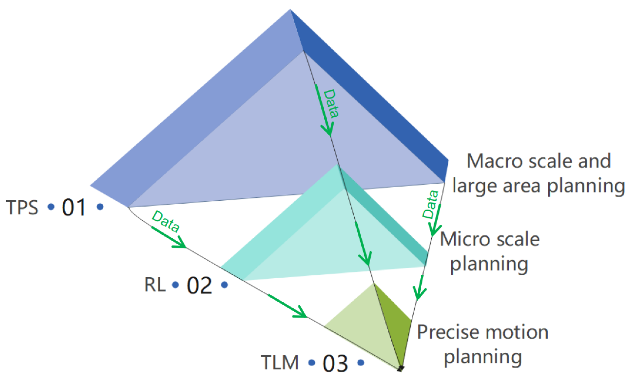
To settle the mentioned problems, we first propose a planning hierarchy framework with three levels, as shown in
Figure 1. The first level is for macro-scale planning via TPS, and the second level is the RL method used for micro-scale planning; the differences between macro-scale and micro-scale planning can be found in reference [
15]. The third level is TLM, which can make motion planning more precise and closer to actual environments. Second, we take into account that solving the interpretability and instability problems of deep learning (DL) is difficult because DL’s ability is known, but its operations are unknown. Thus, from the perspective of the traditional methods, TPS and TLM are leveraged to ensure safety and to constrain the RL search space, where motion planning can be stabilized by combining their advantages and overcoming their shortcomings. Third, for uncertain environments such as an uncertain obstacle, RL is used to explore dynamic and uncertain environments, and then multiple constraints are considered and the safety range is set through a safe TPS buffer.
The contributions of our proposed method and model are as follows:
The RLTT method along with a theoretical analysis is proposed for automated driving, in which a novel planning hierarchy framework of three levels and a multi-scale planning based on TPS, RL, and TLM are introduced.
Multiple constraints of vehicles are considered, such as the dynamic constraints of vehicles, smooth constraints, and safety constraints, thereby making motion planning more reasonable and closer to actual scenarios.
Uncertain environments are also considered in the proposed planning method, which achieves superior performance as compared to related works.
Safe and efficient motion planning for automated driving is achieved. The RLTT method, by combining traditional methods and RL, can perform well under sparse information environments and multi-scale planning environments.
The remainder of this paper is organized as follows: Related works are introduced in
Section 2; the dynamic model of a vehicle is provided in
Section 3; TLM is presented in
Section 4; the method of TPS is introduced in
Section 5; the RLTT method for automated driving is introduced in detail in
Section 6; related experiments are described in
Section 7; the conclusion of the paper is given in
Section 8.
2. Related Work
The planning for unmanned vehicles has attracted a lot of attention in the automated driving community [
16], especially from the perspective of data-driven methods in complex environments which are unknown and uncertain.
For example, in [
17], Bernhard and Knoll considered uncertain information using neural networks for automated vehicle planning. Nevertheless, they assumed all information about other vehicles to be known, and that this assumption might not be suitable for real environments. Zhang et al. [
18] developed a novel bi-level actor–critic method for multi-agent coordination. Although their method achieved great success in making quick decisions regarding automated driving in highway merge environments, this method could not guarantee the safety of automated vehicles. Nick et al. [
19] introduced an algorithm for clustering traffic scenarios, in which they combined convolutional neural networks and recurrent neural networks to predict traffic scenarios for the ego vehicle’s decision-making and planning. However, their method might be unstable for some extreme traffic scenarios because of the uncertain and imperfect information on some traffic situations, such as intersection environments. In [
20], a safe motion planning for autonomous vehicles based on RL and Lyapunov functions was proposed, where the reward function was optimized with respect to agent safety, and the balance between reward and safety was analyzed by optimizing the probability of collision. Similarly, uncertain environments were also not considered.
Chen et al. [
21] developed an end-to-end method for automated driving using RL and a sequential latent environment model, which is a semantic bird-eye mask; their methods were more interpretable than other machine learning methods to some extent. However, their method may still need to further consider sparse information environments and multiple constraints for automated driving. Tang et al. [
22] introduced a motion planning method for automated driving using a soft actor-critic method [
23], in which different strategies were balanced via the weights of safety, comfort, and efficiency. Zhu et al. [
24] developed a motion planning method to consider the factor of pedestrian distraction based on a rule-based method and a learning-based method. Their experimental results demonstrated that the learning-based method may be better at handling the unsafe action problem at unsignalized mid-block crosswalks than the rule-based method; nonetheless, the learning-based method may generate unreasonable actions. Wen et al. [
3] provided a safe RL method for autonomous driving based on constrained policy optimization, in which the risk return was considered as a hard constraint during the learning process, and a trust region constraint was used to optimize the policy. Although they achieved better performance than CPO [
25] and PPO [
26] in some scenarios, their method considered risk as an optimization objective based on neural network learning. This learning process might encounter violations of the safety constraint, which will not allow for safety to be achieved with high confidence. In contrast to their methods, our method is based on a geometry reachability analysis and vehicle dynamic verification, which can guarantee safety during automated driving.
Shai et al. [
27] presented a sophisticated strategy based on RL which considers negotiation strategies when the ego vehicle drives in complex environments. Their method can be divided into two strategies: one strategy that can be learned, and another strategy associated with hard constraints that cannot be learned (e.g., safety constraints). Although they tried their best to ensure the safety of automated driving, their method still required an improvement in adaptability for more complex environments such as a complex intersection with multiple heterogeneous vehicles and pedestrians. Sarah M. Thornton [
28] proposed a method that leveraged the Markov decision process (MDP) and dynamic programming to control the vehicle speed for safety, and this method considered uncertain pedestrians at a crosswalk. However, the method might require improvements in order to consider more uncertain environments, and the search space may need to be reduced for efficient planning. Codevilla et al. [
29] used condition imitation learning for a high-level command input to achieve automated driving in simulation environments and for a 1/5-scale robotic truck in real environments. Although both experiments evaluated the effectiveness of their method, the method may need to address the need of automated vehicles for human guidance in sparse information environments.
Moreover, there are many alternative methods available for solving robot motion planning problems, such as a probabilistic Chekov method for robots that plans via chance constraints [
30], a probabilistic collision constraint planning based on Gaussian probability distribution functions [
31], artificial potential fields for motion planning [
32], symptotically optimal planning for robots on the basis of a rapidly exploring random tree (RRT) [
33], direct sampling for robot path planning derived from RRT [
34], a fast marching method for path planning [
35], etc.; although the above methods have shown impressive progress in robot motion planning research, the methods may need to be further developed for autonomous driving and consider the features of vehicles and autonomous driving environments.
In this paper, the proposed RLTT is different from the above-mentioned methods because it can achieve safe and efficient automated driving in sparse information environments while considering multi-constraint and multi-scale motion planning.
In RLTT, TLM is developed on the basis of the trajectory unit, which was first proposed for unmanned surface vehicles (USVs) [
36,
37,
38]. However, USVs are different from automated vehicles. The freedom of control, navigation environments, and vehicle shapes are different [
15,
39]. The trajectory unit may not be suitable for automated vehicles, therefore developing TLM for automated vehicles is necessary. Moreover, TLM is different from a lattice planner[
40] because a lattice planner is achieved using sample and fit data, which may require a huge amount of time and more computing power. In contrast, TLM is achieved via a dynamic model of vehicles in advance. In addition, TPS is proposed to constrain the RL search space and provide routing points for RL navigation, which can improve RL efficiency. Finally, the hierarchy framework is proposed by integrating TPS, RL, and TLM to develop the RLTT method, which can make the proposed method and model more unified.
3. Problem Formulation
In this study, a constrained RL problem is considered for motion planning; in particular, uncertain constraints , dynamic constraints , safety constraints , and smooth constraints are considered.
3.1. Uncertain Constraints
For the convenience of description, we have provided the following definitions for (
1):
denotes the obstacles;
denotes the shape of the obstacles;
denotes the position of the obstacles;
denotes partial information about the obstacles’ positions and shapes.
Definition 1. In uncertain environments, since information about an obstacle shape cannot be fully observed, is used to denote partial information about the obstacles that the agent observes. 3.2. Dynamic Constraints
Dynamic constraints
can be defined as the dynamic model of vehicles, which is briefly shown in
Figure 2. In this paper, a kinematics model, steer command, and heading angle are considered. The kinematics model is briefly introduced in this study [
41,
42]. In general, the steer command range is set to approximately
, or to
for other settings, and the setting of the steering command of our method is suitable for and can be applied to real vehicle experiments.
The driving speed at the axle center of the rear axle is
.
represents the coordinates at the axis of the rear axle, and
represents the heading angle.
The kinematic constraints of the front and rear axles are as follows:
represents the front wheel steering angle, which is similar to the steering command, and it is used to name the steering command here.
where
l indicates the distance between the rear axle and the front axle (wheelbase),
w represents the yaw rate, and
R denotes the turning radius of the vehicle. The geometric relationship between the front and rear wheels is as follows:
According to the analysis above, the kinematic constraints can be briefly summarized in Equation (
6):
3.3. Safety Constraints
The safety distance is , and the distance between the point of motion planning and obstacles is .
Definition 2. The safety constraints () are represented by Equation (7): 3.4. Smooth Constraints
The motion planning points are represented by the set P, . The two adjacent points are and . The two-steer angle difference of any two adjacent points is . The limitation of the two-steer angle difference of any two adjacent points is , where is set to smoothen the steer angle.
Definition 3. The smooth constraints can be represented by Equation (8): In conclusion, we need to find a proximal optimal motion planning set for vehicles that can also simultaneously satisfy the constraints , and .
Definition 4. The objective needs to satisfy the following constraints, which can be formulated as follows: 5. Topological Path Search for Automated Driving
For a large-scale and efficient path search, a topological map meant for high path search efficiency is constructed [
46,
47]. During the path searching process, the open geospatial consortium (OGC) is used to make a topological map [
48]. OGC defines a simple feature model that is suitable for efficiently storing and accessing geographic features in relational databases.
A spatial map comprises nodes, lines, and a surface, which are three elements for constructing a map: a node is a point that does not have spatial features such as shape and size; a line comprises a series of nodes, whose spatial features include shape, length, etc.; the surface comprises closed rings, whose spatial features include shape, area, etc. In TPS, a node denotes the vehicle, a line denotes the routing path, a surface denotes the obstacles.
Spatial relationship refers to the spatial characteristic relationship between geographical entities, which is the basis of spatial data organization, query, analysis, and reasoning. It includes topological, metric, and direction relationships. Numerous topological relation expression models have been proposed to represent spatial relationships. In this study, the nine-cross model [
48] is used to represent the space topological relationship used for the construction of a topological map. This is introduced through Function (
29), where A and B represent two different objects,
denotes the edge of an object,
denotes the internal part of an object,
denotes the external part of an object, and
denotes the intersection of two objects.
Based on Function (
29), the topological relation predicates are defined, which are Crosses, Disjoint, Within, Contains, Equals, Touches, Intersects, and Overlaps. In this paper, we leverage Intersects, Disjoint, Touches, and Contains to analyze the topological relationship shown in
Figure 8. For example,
denotes the Disjoint;
,
, and
denote Touch;
and
denote Contains/Within;
,
,
, and
denote Intersects via the nine-cross model. For two objects in space, a and b, the intersection value
is denoted by F (False), the value
is denoted by T (True); the intersection is represented by 0 when the point is the intersection, by 1 when the line is the intersection, and by 2 when the area is the intersection. * means that f, 0, 1, or 2 can be selected. More specifically, a. Disjoint b means two geometric bodies (a and b) have no common intersection, thus forming a set of disconnected geometric shapes.
After constructing the topological map, the Dijkstra algorithm [
49] is used to achieve an optimal routing planning, and the Euclidean metric is used to measure the distance between two points, which is provided by Function (
30). The algorithm is described in Algorithm 2, in which Function (
29) is used to judge the topological relationship between obstacles
, the start point
S, and the end point
E; Function (
29) is used to judge the topological position relationship between the path point and each point
of the
ith obstacle
.
In addition, the safety buffer is set according to topological relationships. Moreover, the routing path can be achieved by the Dijsktra algorithm using Function (
30) based on the constructed topological map; the Dijskra algorithm can achieve a more optimal path than other heuristic algorithms, e.g., the A* algorithm, even though it requires more computing time. However, in this study, the Dijskra algorithm based on TPS could quickly find the optimal path and satisfy motion planning constraints.
According to the size of the vehicle maneuver, the size of the safety buffer is set at 8 (m), which indicates that the distance between the path and the obstacles is always 8 (m), thus making the route planning safe and suitable for motion planning.
| Algorithm 2: The method of TPS for automated driving. |
![Robotics 11 00081 i002]() |
6. A Motion Planning Method for Automated Driving
TLM and TPS were constructed in the previous sections. In this section, we will discuss how to achieve motion planning for automated driving. RL is briefly introduced [
8], the RLTT method for automated driving is then presented in detail, and multiple constraints are considered in the RLTT method.
TPS is introduced for large and macro-scale motion planning, in which both driving safety and optimal path planning are achieved via a safety buffer, a topological map, and the Dijkstra algorithm. A representation of TPS constraints is given in
Figure 9a. For micro-scale motion planning, in which the environment contains uncertain and imperfect information, building a model and learning experiences via a data-driven method is easier than traditional methods; in contrast, when the environment is uncertain, the environment is difficult to model via traditional methods.
Figure 9b shows the representation of constraints through RL. TLM can be used for dynamic constraints and smooth constraints, in which the kinematic model of vehicles and steer constraints as well as the relative angle between any two adjacent points are also limited; the representation of TLM is given in
Figure 9c. Considering this type of framework and environment is useful because the perfect environment information cannot be obtained in a real environment even if advanced sensors are used. The proposed method could aid in the advancement of automated driving.
6.1. RL Methods
RL can be typically regarded as MDP, and MDP is presented by a five-object tuple , where S denotes the state space, A denotes the action space, P shows the probability of transition, R represents the reward once one action is performed, and denotes the discounted factor of the reward. In this study, RL is regarded as the partial observation MDP, where RL makes an agent interact with the environments through trial-and-error learning in order to obtain more data about the environments, and the agent can then learn better about the environments as well as perform better. In particular, RL can deal with uncertainty problems better than traditional methods. Notably, the most likely action can be selected in the future environment on the basis of previous exploration. It can reduce the uncertainty about the environment, which means that more knowledge can be acquired about the environment, and more certain information can be obtained for future decision making.
6.2. A Motion Planning Method
First, the TLM and TPS are introduced into the framework, and Q learning is developed based on the TLM and TPS, providing the constrained RL for safe motion planning.
Second, the transition function f of Q learning is integrated into TLM and TPS. More specifically, for the transition function f, the input is action a, the current position is , the angle is A, and the terminal is ; the output is the next position , the reward is r, done is T, and the next angle is . The transition process is as follows: If the current position has collided with an obstacle , then return the state s, reward r, done, and angle A; if the current position has reached the terminal , then return state s, reward r, done, and angle A; at the same time, if angle A and action a are equal to angle and action of the trajectory, respectively, we can obtain the next position ← current position , next angle ← angle A, and obtain the related reward r. If the next position has collided with an obstacle , then return the state s, reward r, done T, and angle A; if the next position has reached the terminal , then return the state s, reward r, done T, and angle A. Iteratively proceed according to this logic, obtain the related path information, and return each position’s next position , reward r, done T, and next angle for further motion planning.
Third, the algorithm of Q learning is presented for the path value, which can be seen in Algorithm 3. Finally, according to the distance of the safety buffer, select the routing points and call Algorithm 4 for the automated driving motion planning.
| Algorithm 3: Q learning method for the path value. |
![Robotics 11 00081 i003]() |
| Algorithm 4: Motion planning for automated driving via RLTT. |
![Robotics 11 00081 i004]() |
6.3. Motion Planning Examples
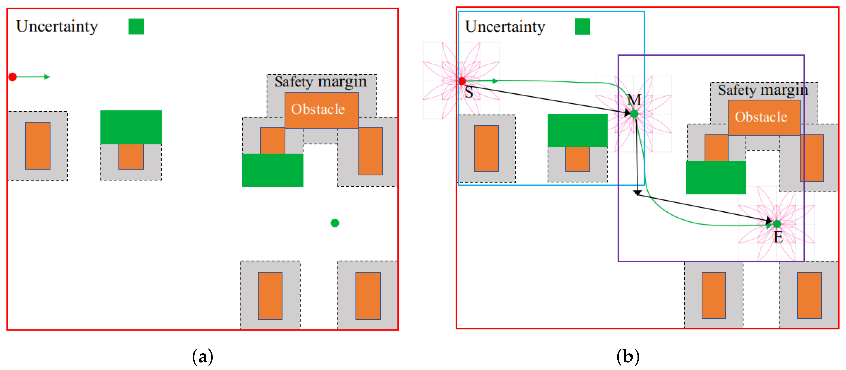
A motion planning example of automated driving via RLTT is illustrated in this section. The problem of motion planning in certain and perfect information environments may be easy to solve using the traditional methods such as the sample-based method. However, if uncertain environments and vehicle constraints are considered, the traditional methods may not perform well. For example, in
Figure 10a, the red circle point represents the start point, the green circle point represents the end point, and the green arrow represents the dynamic constraints, including the heading constraints and steer constraints, among others. When the environment is
certain and
uncertain, for example,
of the obstacles expand randomly upward or downward by
. More specifically, the position and shape of 65% of the obstacles are certain, and the position and shape of 35% of the obstacles are uncertain. When the vehicle is navigating, 35% of the obstacles change at random. The RLTT method can perform well in the environments because it can efficiently and rapidly explore the unknown world in micro-scale motion planning (blue box (from the S point to the M point) and purple box (from M point to E point)). More specifically, it leverages TPS for large and macro-scale routing planning (red box (represented by the black arrow from the S point to the E point)) and TLM for micro and precise motion planning (deep pink line). An example is given in
Figure 10b, with the motion planning trajectory represented by the green arrow from the S point to the E point. Furthermore, we provide the complexity analysis of RLTT in Remark 1.
Remark 1. The proximal optimal search time for motion planning with a constrained RL is as follows:
The search time for TPS is , where M represents the number of obstacle points; for the RL search time, the complexity is , where T is the total number of steps [50]. More particularly, the convergence of our method can be guaranteed based on the Banach fixed-point theorem [
51]; for the detailed convergence proof of the constrained RL, see [
52].
7. Experiments
Several experiments were conducted in the same environments, and the results are analyzed here in detail. First, different RL methods for path search were tested. Second, the RLTT method for motion planning was achieved for automated driving. Third, comparison experiments in certain and uncertain environments have been carried out. In addition, comparison experiments between RLTT and RL algorithms were provided. Fourth, comparison experiments between RLTT and traditional algorithms were conducted to evaluate the effectiveness of our proposed methods. Finally, RLTT for automated driving motion planning in uncertain corridor environments was carried out to demonstrate our method’s applicability.
Moreover, all experiments were run on an Ubuntu 18.04 system (Dell PC), in which the CPU was an Intel Core i7-9750H CPU 2.60 GHz × 12, the GPU was an Intel UHD Graphics 630 (CFL GT2), the Memory was 31.2 GB; all comparison experiments were conducted under the same environment conditions, and the computation time in the experiments included training time and test time. The number of initial iteration steps was 10,000, the learning rate was , the epsilon value of the maximizing optimal value was . For the reward settings, we set them on the basis of the safety cost, distance cost, and steering cost of the vehicle. If the vehicle collided with obstacles, the reward was ; if the vehicle found the target position with the correct attitude, the reward was 10; the reward for each step the vehicle took along the straight line was ; for each step the vehicle took along the diagonal direction, the reward was ; for each step the vehicle took along the oblique curve, the reward was ; the reward was for every turn in the steering action; if the vehicle took each step along the diagonal and straight direction, the reward was .
7.1. Different RL Methods for Path Search
Related RL methods for conducting the path planning for automated driving have been performed, which can be seen in
Figure 11. The figure shows that the dynamic programming (DP) value and policy iterations [
8] achieved fewer steps, implying that the two algorithms can obtain the shortest path for automated driving. Nonetheless, DP value and policy iterations may be unsuitable for automated driving in uncertain and unknown environments because the probability and reward transition might not be known, and the above two methods typically need information regarding the model of environments.
In addition, the Monte Carlo (MC) RL method [
8] achieved almost the same number of steps as the Q learning [
53] for automated driving. However, the MC method sometimes falls into a deadlock during exploration and cannot obtain the desired path due to the complex environments. The Sarsa method [
54] obtains more steps than Q learning because of its conservative strategy. Because RLTT is a multi-scale method and the safety buffer constraints of the first level via TPS have been further considered, it is better to develop Q learning and integrate it into the RLTT framework for automated driving. In the next section, the experiments of the RLTT method for automated driving are introduced and discussed.
7.2. A RLTT Method for Motion Planning
7.2.1. Macro-Scale Motion Planning
In this section, macro-scale planning (generally, the planning area can be set from approximately 100 to
(m)) was accomplished via TPS (
Figure 12a,b), which represents the convex obstacle and concave-convex obstacle environments, respectively, in which the macro-scale planning is represented by the deep pink line and the obstacles are represented by the red rectangles. The start point and end point are
S and
in
Figure 12a and
and
in
Figure 12b, respectively. The safety buffer was set at 8 m, as shown in
Figure 12a,b (denoted by
B and the yellow arrow).
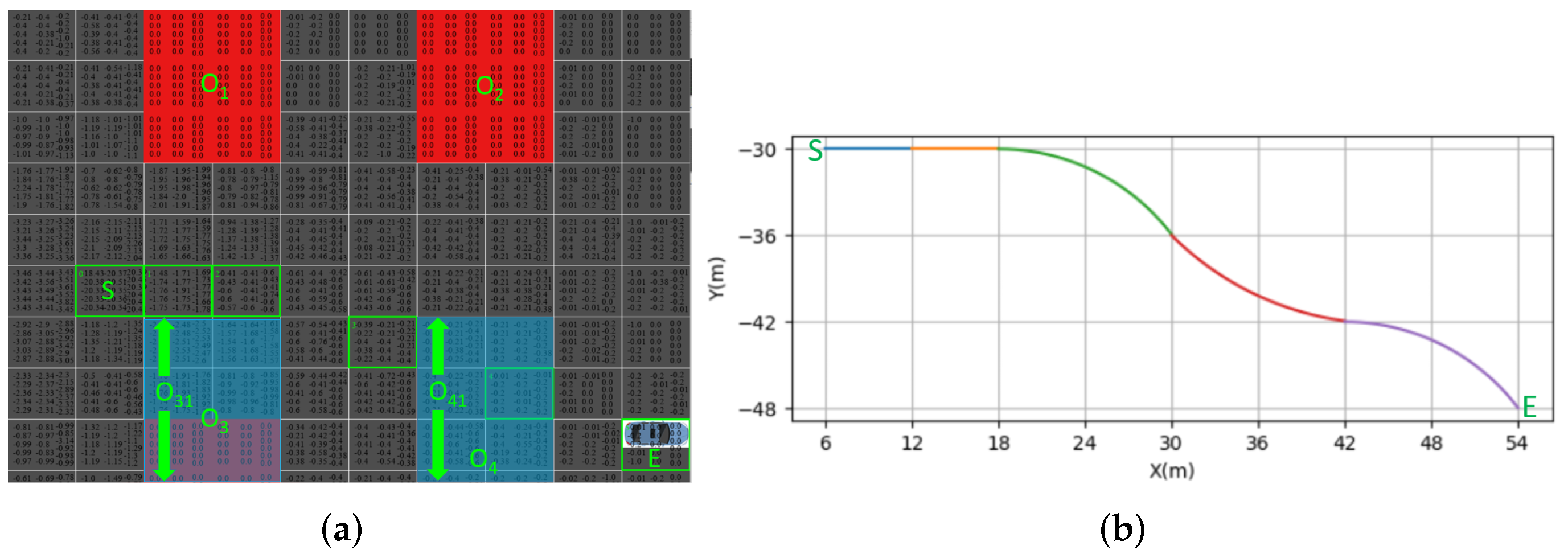
7.2.2. Micro-Scale Motion Planning
The micro-scale motion planning (generally, the planning area can be set at approximately 100 m) was achieved, as shown in
Figure 13 and
Figure 14, where the environment information is unknown. The start point is the
S point and the end point is the
E point. The obstacle is denoted by
O. RL was constrained by TPS and TLM, and it was used to dynamically explore the suitable point from the
S to the
E points. TLM was used to splice the RL points, where the smooth and dynamic constraints were considered; the two bottom obstacles randomly changed within a certain range. In particular, obstacles
and
randomly changed within the
and
ranges (as shown in the light blue rectangles); therefore, the motion planning is different in
Figure 13 and
Figure 14.
7.3. Comparison Experiments in Certain and Uncertain Environments
Related experiments were conducted in different environments, which were either certain (known environment information) or uncertain environments (unknown environment information), as shown in
Figure 15. The environments were the same except for the random obstacles. The average distance of five uncertain experiments was
(m), and the average distance of five certain experiments was
(m). The experiments showed that the RLTT method could deal with the uncertain environments well.
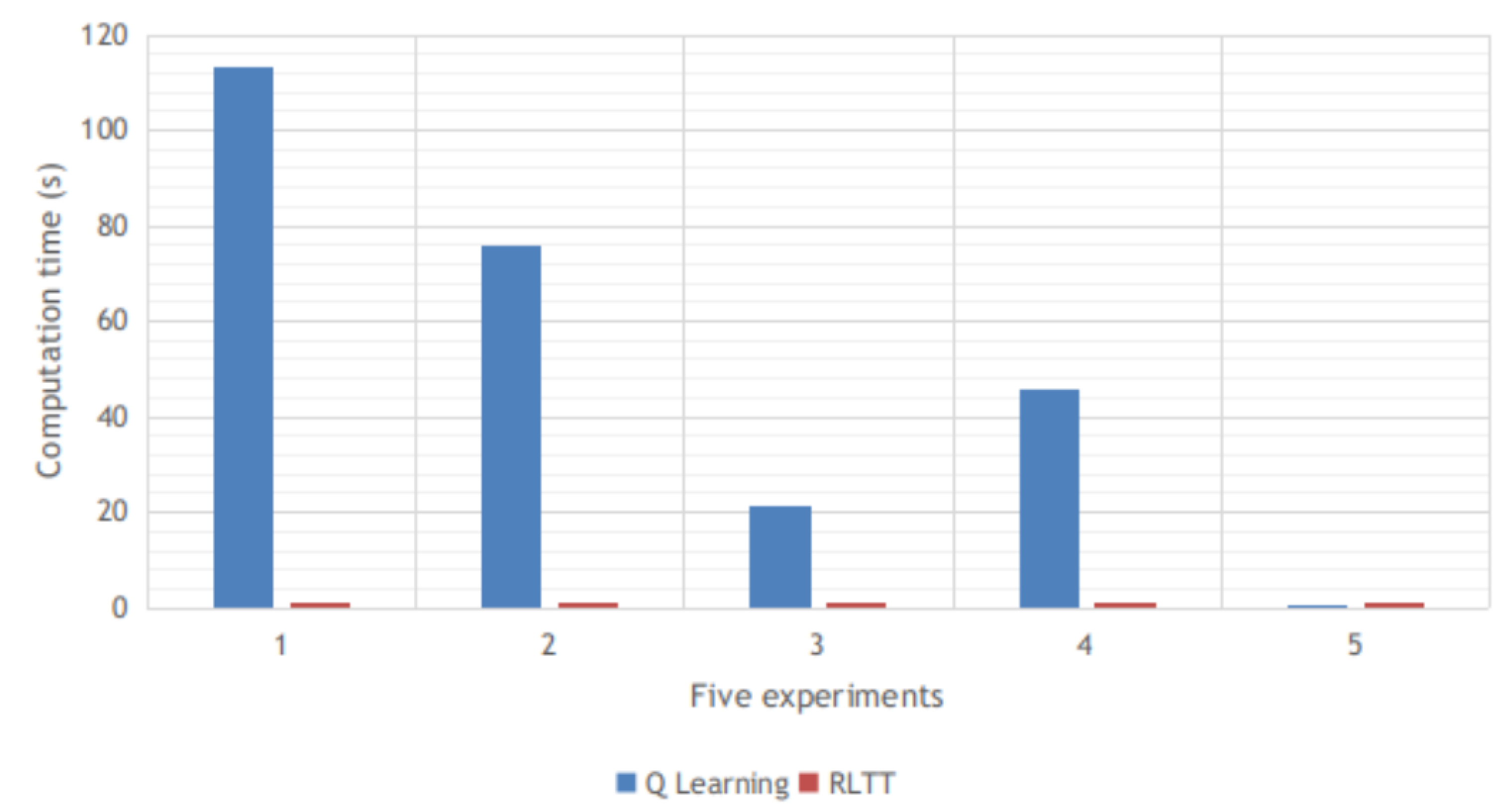
7.4. Comparison Experiments between RLTT and Q Learning Algorithms
We conducted five experiments using the RLTT method and the Q learning algorithm in unknown environments. The Q learning algorithm is a classic and commonly used algorithm for vehicle navigation. The computation time of each experiment and the averaged computation time of the five experiments using the RLTT method and the Q learning algorithm are shown in
Figure 16 and
Figure 17, respectively.
More specifically, the averaged computation times for the RLTT method and Q learning for motion planning were 0.325 (s) and 52.279 (s), respectively. In addition, the trajectory distance when using Q learning is usually greater than that when the RLTT method is used. We randomly selected one of the five experiments and computed the trajectory distance. The distance when using the RLTT method was 95.834 (m), whereas that when using the Q learning algorithm was 126.735 (m). The results indicate that the performance of the RLTT method was better than the classic RL algorithm, and the RLTT method achieved a shorter trajectory distance and used less time for the path search as compared to the classic RL algorithm.
7.5. Comparison Experiments between RLTT and Traditional Algorithms
This section shows the experiments comparing the RLTT and traditional algorithms for automated driving motion planning. The adopted traditional algorithm is a hybrid A* algorithm [
55], which was proposed by Dolgov et al. It was developed based on the A* algorithm [
39] by leveraging continuous coordinates to guarantee the kinematic feasibility of the trajectories and the conjugate gradient descent in order to improve the quality of the trajectories on the geometric workspace. The hybrid A* algorithm has shown better performance than the rapidly exploring random trees algorithms [
56,
57] and the parameterized curve algorithms [
58] in terms of fast global convergence and optimal global values. It is very useful and widely used for automated driving since the hybrid A* algorithm can be smooth and practical for autonomous driving in real-world and unknown environments [
55].
The distance of motion planning using the RLTT algorithm was 147.4 (m), which considered dynamic constraints under the environments with sparse information; on the other hand, in the same environments, the distance of motion planning using the hybrid A* algorithm while considering dynamic constraints was 184.0 (m). The experimental results indicate that our proposed method outperforms the hybrid A* algorithm in terms of distance.
7.6. Uncertain Corridor Scenarios
We referred to the experimental settings of reference [
59] to carry out an experiment on uncertain corridor scenarios.
Figure 18a shows real traffic environments: uncertain corridor scenarios.
Figure 18b shows motion planning via RLTT for an automated vehicle in real and uncertain traffic scenarios. The red areas denote uncertain objects, where there is a corridor, some vehicles, and pedestrians crossing the corridor uncertainly. The vehicles on the main road (as indicated by the light blue arrow) can safely cross the uncertain corridor scenarios; the distance of motion planning was 61.8 (m).


