Sensor Fusion with Deep Learning for Autonomous Classification and Management of Aquatic Invasive Plant Species

Abstract

Recent advances in deep learning, including the development of AlexNet, Residual Network (ResNet), and transfer learning, offer unprecedented classification accuracy in the field of machine vision. A developing application of deep learning is the automated identification and management of aquatic invasive plants. Classification of submersed aquatic vegetation (SAV) presents a unique challenge, namely, the lack of a single source of sensor data that can produce robust, interpretable images across a variable range of depth, turbidity, and lighting conditions. This paper focuses on the development of a multi-sensor (RGB and hydroacoustic) classification system for SAV that is robust to environmental conditions and combines the strengths of each sensing modality. The detection of invasive Hydrilla verticillata (hydrilla) is the primary goal. Over 5000 aerial RGB and hydroacoustic images were generated from two Florida lakes via an unmanned aerial vehicle and boat-mounted sonar unit, and tagged for neural network training and evaluation. Classes included “HYDR”, containing hydrilla; “NONE”, lacking SAV, and “OTHER”, containing SAV other than hydrilla. Using a transfer learning approach, deep neural networks with the ResNet architecture were individually trained on the RGB and hydroacoustic datasets. Multiple data fusion methodologies were evaluated to ensemble the outputs of these neural networks for optimal classification accuracy. A method incorporating logic and a Monte Carlo dropout approach yielded the best overall classification accuracy (84%), with recall and precision of 84.5% and 77.5%, respectively, for the hydrilla class. The training and ensembling approaches were repeated for a DenseNet model with identical training and testing datasets. The overall classification accuracy was similar between the ResNet and DenseNet models when averaged across all approaches (1.9% higher accuracy for the ResNet vs. the DenseNet).

1. Introduction

Recent advances in machine learning frameworks, namely, deep learning, and the advent of general-purpose parallel processing architectures have created a new paradigm for remote sensing. Neural networks as a machine learning framework are unique as compared to classic techniques in their ability to, via adaptation of network parameters (weights), provide robust function estimation. In fact, it has been shown that a sufficiently wide, single-layer neural network using a sigmoid nonlinearity can approximate any continuous function [1]. By selecting the correct weights, a neural network can perform regression or classification tasks with great accuracy on high-dimensional data. The process of using data to perform optimization of network weights is referred to as training.

The computer vision field has advanced significantly since the introduction of AlexNet in 2012. This neural network utilized five convolutional layers, trained on a graphics processing unit (GPU) to achieve what was then state-of-the-art performance on image recognition and classification tasks [2]. Since this proof of concept, much research has been conducted in the realm of machine vision, that has resulted in neural network architectures that far outperform AlexNet for machine vision tasks. Research has revealed that convolutional layers act as feature detectors, and increasing the number of stacked convolutional layers (the network depth) enables better network performance [3]. Furthermore, it was discovered that while neural networks are valued for their function estimation capabilities, they often fail to estimate an identity function. The introduction of residual units via skip connections between layers was presented as a partial solution to this problem, enabling the training of even deeper convolutional networks [4].

While deep convolutional neural networks exhibit state-of-the-art performance on machine vision tasks when properly trained, the training process is computationally intense. The original AlexNet network contained over 60 million tunable weights and took 5–6 days to train [2]. Adding more convolutional layers to increase the network depth generally serves to increase the number of weights in the network. In addition, increasing the weight count of a network requires more data for the network to train on, to prevent overfitting of the network to training data and improve generalization. Thus, there exists an inherent tradeoff between the ultimate performance of a neural network and the difficulty of training.

Transfer learning, inspired by the psychology of human learning, aims to reduce the computational and dataset requirements necessary to generate well-trained neural networks by applying knowledge gained from past experiences to new learnings in a similar domain [5]. A practical example of transfer learning in the field of machine vision can be seen in convolutional filters. As mentioned, each convolutional layer of a network acts as a feature detector. Features are aggregated as they pass through successive layers, enabling emergent features, such as the presence of an object, to be constructed from low-level features such as the presence of an edge or corner. The features output from the final convolutional layer can then be used to classify an image. This enables pretrained convolutional layer filters to be shared between image classification tasks, as features such as edges, corners, and shapes are generally shared between all images. Transfer learning has shown great success in the domain of autonomous weed control. Classification of RGB images of eight in situ invasive plant species using transfer learning of a ResNet-50 convolutional network achieved a test accuracy of 95.7% on a dataset comprising 17,509 images [6].

Continual learning, also referred to as lifelong learning, has emerged in recent years and seeks to autonomously augment network training over time, without retraining over prior data. A challenge to continual learning is the loss of prior knowledge, which can lead to catastrophic forgetting. Rostami et al. developed a continual learning computational model that generates pseudo-data points to replay past experiences, thereby addressing catastrophic forgetting [7]. Jha et al. applied continual learning to human activity recognition [8]. Ashfahani et al. proposed an autonomous deep learning methodology, featuring a self-constructing network structure [9], while Li et al. proposed an immune-system-inspired classification method [10].

Machine learning also has direct applicability to the management of aquatic invasive plants (AIPs). Work by Patel et al., utilizing AlexNet, revealed that deep neural networks can accurately classify submersed aquatic vegetation (SAV) captured in hydroacoustic imaging [11]. Non-native AIPs, such as Hydrilla verticillata (L.f.) Royle (hydrilla), promote adverse situations among native aquatic environs and the related infrastructure within invaded waterways. Since AIPs generally lack natural predation, once established, they reduce aquatic ecosystem biodiversity through resource competition, displacement, and habitat disruption of native flora and fauna [12]. Further, the monetary hindrance associated with AIPs is equally noteworthy, since invasive aquatic weeds regularly inhibit recreational boating activities, obstruct drainages, limit municipal and hydropower water supply, and can reduce waterfront property values [13]. In the United States alone, greater than 100 million dollars (USD) are spent annually for the management of AIPs [14].

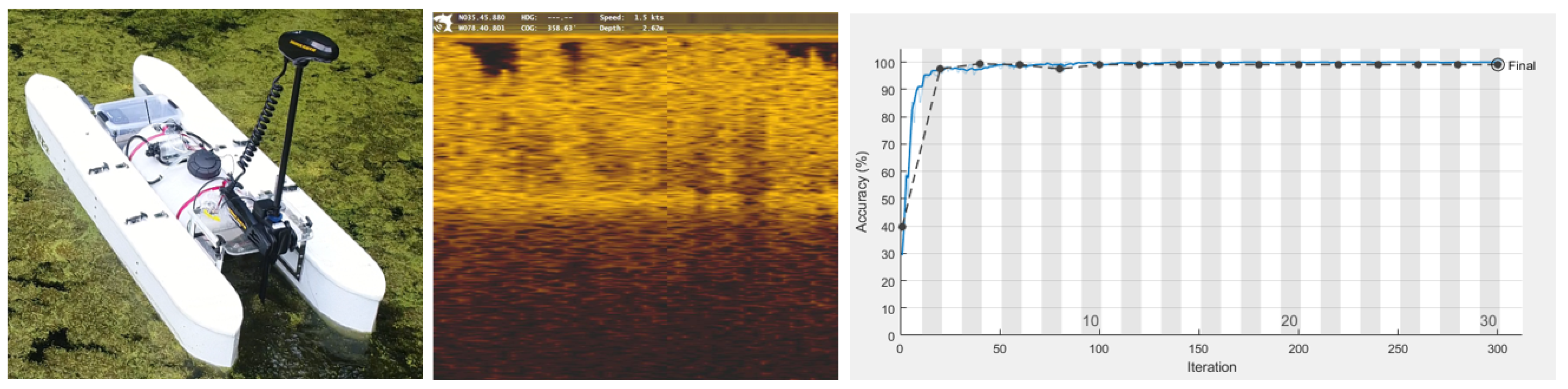
Aquatic resource management frequently relies on well-timed monitoring and mapping strategies to gauge the presence and abundance of AIPs. In the United States, boat-based point-intercept sampling protocols remain the standard for documenting the spatiotemporal patterns in the occurrence and distribution of AIPs within invaded waterbodies [15]. However, AIP assessments require a skilled survey crew and substantial time to complete a comprehensive survey, and the precision and scale of these surveys is highly dependent upon the time spent evaluating each sample point location. To overcome the aforementioned hindrances of point-intercept surveys, AIP practitioners are actively pursuing recent advances in off-the-shelf remote sensing and photogrammetric technologies, specifically sUASs (small Unmanned Aircraft Systems) and sonar-equipped aquatic drones. Recent work has focused on the development of a small fleet of fully autonomous boats (Figure 1) capable of subsurface hydroacoustic imaging and herbicide deployment (for vegetation control) [11]. These multihulled vehicles, with a single on-shore operating station, have been tested in a variety of weather conditions and have demonstrated reliable, accurate tracking performance with little to moderate wind (4.5 m/s, 10 mph), extended battery life (estimated at 8 or more hours), and operation speeds of up to 2.3 m/s. Machine learning classification algorithms, developed as a component of this research, achieved a classification accuracy of 99.06% after training on four fully submersed plant species categories (hydrilla, Cabomba caroliniana A. Gray (cabomba), Ceratophyllum demersum L. (coontail), or “other”). However, these algorithms could not effectively process data from floating vegetation or SAV at the surface of the water column (i.e., “topped out”), since the structure of the plant canopy was above the sensing view of the hydroacoustic sensor in these cases.

Despite the potential to reduce expenditures associated with AIP surveys, sUAS-based true-color (RGB) cameras and hydroacoustic (sonar) sensing technologies have limitations regarding the classification of SAV; neither is consistently proficient at producing robust, interpretable imagery with variable depth, turbidity, SAV biovolume (percent of water column occupied with SAV), and poor light conditions. However, each sensing technology does provide unique opportunities to overcome specific deficiencies of the other. For example, hydroacoustic sensors can provide a clear view of the lakebed (benthos) and are unimpeded by environmental factors such as sun glint and turbidity. Unfortunately, the spatial resolution of hydroacoustic sensing is low, limiting the ability to distinguish plant features and sense at, or near, the surface of the water column. Conversely, aerial RGB sensing provides high-resolution images of the upper portion of the water column but is highly impeded by environmental conditions, specifically water column turbidity, wave action (fetch), and sun glint.

Fusing the sensing capabilities of sUASs and aquatic drones could exploit the strengths of each modality for improved SAV classification accuracy. The objective of this work is to integrate neural networks, incorporating both hydroacoustic and aerial RGB imagery, for real-time classification of SAV. Methods will utilize transfer learning, via a ResNet-50 model, with weights pretrained on the ImageNet dataset.

2. Materials and Methods

2.1. Training Set Image Generation

Aerial RGB images were acquired during monthly surveys of Lake Mann (Orange County, FL, USA) and Lake Sampson (Bradford County, FL, USA) using a quadrotor-type unmanned aerial vehicle (UAV, SZ DJI Technology Co., Ltd., Shenzhen, China). Images from each survey were stitched into orthomosaic images of each lake using commercial software (DroneDeploy, San Francisco, CA, USA). The orthomosaic images were then downloaded with a ground sampling distance (GSD) of 3 cm and processed using the Mapping toolbox of MATLAB R2021a (MathWorks, Natick, MA, USA). Each orthomosaic and associated GPS positional data were converted into an array of indexable RGB pixel values. Figure 2 shows the fully processed orthomosaic of one survey on Lake Mann. The monthly surveys of Lake Mann and Lake Sampson included hydroacoustic imaging in concert with the RGB image collection. Hydroacoustic data collection was conducted using a boat-mounted Lowrance sonar unit (Navico, Egersund, Norway) integrated with GPS (±2 m accuracy) and the transducer set at 10 pings per second at 200 kHz with a 12° cone aimed in the nadir position. Individual hydroacoustic images were generated from sonar data, as in [11].

Aquatic vegetation was identified at the species level via point grid surveys, with SAV destructively sampled using a modified four-tine rake on an extendable pole at each georeferenced point. Abundances were scored qualitatively with a rank of 1–3 based on “rake fullness” according to the protocol developed by Hauxwell et al. [16]. Data attributes were transferred via cellular network communication and stored electronically. The point intercept data were partitioned into three main groups: those noted to contain hydrilla, those that contained aquatic species without hydrilla, and those with no aquatic vegetation. Each set of georeferenced points was processed via a MATLAB script to find the nearest neighbor of the RGB geospatial data. Finally, 256 × 256 images were cropped from the RGB grid, centered at the indexes found to be closest to the point grid locations. Labels were generated for each image: “HYDR” for images of point grid locations where hydrilla was found, “OTHER” for images that contained aquatic vegetation but not hydrilla, and “NONE” for images that contained no aquatic vegetation. Data processing in this manner yielded approximately 1000 images per each corresponding orthomosaic/point-grid-survey and required less than 10 min.

2.2. Neural Network Training

Network training was conducted using a multistage approach. First, convolutional neural networks were trained for classification individually on data for RGB images and hydroacoustic images. Of the total image pairs generated, 15% were allocated for testing. The remaining 85% of image pairs were partitioned into 80% for training and 20% for validation. Following [6], a transfer learning approach was employed to enable training of a network with a large number of weights without substantial overfitting. For training, the TensorFlow Keras framework was utilized due to its popularity, ease of development, and the availability of pretrained networks for transfer learning. A ResNet-50 model with weights pretrained on the popular ImageNet dataset was selected as the basis for transfer learning. The convolutional weights were loaded, while the final, multilevel perceptron layer that performs classification on the extracted features was replaced. The pretrained multilevel perceptron layer was replaced with a feature classification pipeline consisting of 2D average pooling, feature flattening, fully connected layers of dimensions 1000 × 10 and 10 × 3, and a final output Softmax layer. During training, the preloaded convolutional weights were frozen, to prevent any changes being made during backpropagation. Training was conducted for a minimum of 25 epochs using the Adam optimizer with a learning rate of 0.001 and early stopping and dropout to lessen overfitting. Figure 3 shows training and validation loss curves for RGB and hydroacoustic neural network training.

The datasets generated for both the aerial RGB images and the hydroacoustic images were unbalanced, with a disproportionate number of images from the “OTHER” class. Using standard log losses for training, the network would likely tend to overpredict the “OTHER” class to minimize training loss. In response to similar unbalanced datasets in computer vision applications, Lin et al. introduced the concept of focal loss, a modification to the standard log loss formulation, $FL\left(p_t\right)=-{\left(1-p_t\right)}^{\gamma }log\left(p_t\right)$, where $p_t$ is the argmax probability [17]. This modification provides a simple method for addressing class imbalance, as the loss contribution of each image in the training set decreases as the prediction confidence increases. Thus, as the network learns to confidently predict classes that make up larger portions of the training set, it becomes increasingly difficult to decrease training loss by increasing accuracy for those classes. For training purposes, focal loss was implemented with $\gamma =5$.

In order to effectively test the fusion of information from hydroacoustic and aerial UAV sensors, a combined dataset must be built that consists of hydroacoustic images and UAV RGB images taken at the same GPS location on the same day. Again, MATLAB was used to generate a set of matching UAV RGB and hydroacoustic images, with test data selected across a range of data collection dates. The RGB dataset was partitioned into a roughly 15% set of test data. For each label (HYDR, NONE, and OTHER), each collection date was selected. Hydroacoustic and RGB image data were read into MATLAB from the dataset, filtered to only select images from the specified date. For each RGB image, the image GPS location was compared against the location for each hydroacoustic image, and distances between candidate pairs were minimized for final RGB/hydroacoustic image pairing. Figure 4 shows examples of paired RGB/hydroacoustic images for test set data. Empirical inspection of the generated pairs of RGB/hydroacoustic images indicates accurate pairing. Aerial RGB images with a clear view of emergent hydrilla are paired with hydroacoustic images that show vegetation reaching the top of the water column. The results stay broadly the same as the plant height observed in hydroacoustic images decreases. As plant height recesses down the water column, the clarity of vegetation in aerial RGB images decreases.

2.3. Multi-Sensor Classification

After generation of test datasets, techniques for fusion of information from aerial RGB and hydroacoustic imagery were evaluated. ResNet-50 networks were trained independently for RGB and hydroacoustic image classification with identical output structures. The independently trained networks were then ensembled to generate the final output. Classic ensemble methods, such as bagging, rely on training multiple neural networks on subsets of the training data and using test-time voting amongst networks to determine the final output. Due to the relatively small training dataset size, partitioning the training data to train multiple models for aerial RGB and hydroacoustic data becomes infeasible. A second technique, stacking, also involves training multiple networks on the subsets of training data. In a stacking approach, multiple base models are trained, after which a fully connected network learns how to fuse the output of these base models. However, this approach requires that a set of validation data be withheld to train the fully connected output model [18]. Because of this, stacking, like bagging, requires larger datasets than were available.

With classic, data-intensive techniques largely infeasible, simpler methods for ensembling of the two networks were considered. First, a simple unweighted average of the two network outputs with the maximum value (TensorFlow “argmax”) of the prediction vector was taken to generate a classification. Secondly, a Monte Carlo dropout (MC Dropout) ensemble was evaluated. MC Dropout presents a means to take advantage of the ensemble properties of the dropout regularization scheme in order to estimate network uncertainty at inference time [19]. In MC Dropout, the dropout procedure of applying a binomial mask to network neurons is applied at inference time as well as training time. The stochastic nature of neuron masking renders the inference process stochastic and enables an estimate of the uncertainty to be generated by performing multiple inferences on the same input data. Weighting of the log-inverse of model uncertainty has shown success in previous work for ensembling of CNN outputs [20]. Third and finally, a logic-based model utilizes knowledge of the advantages and disadvantages of each sensor type. A set of conditional statements is evaluated and used to generate final predictions from the output of each neural network.

3. Results

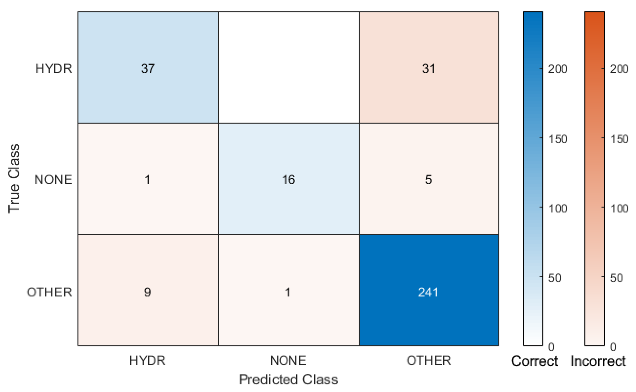
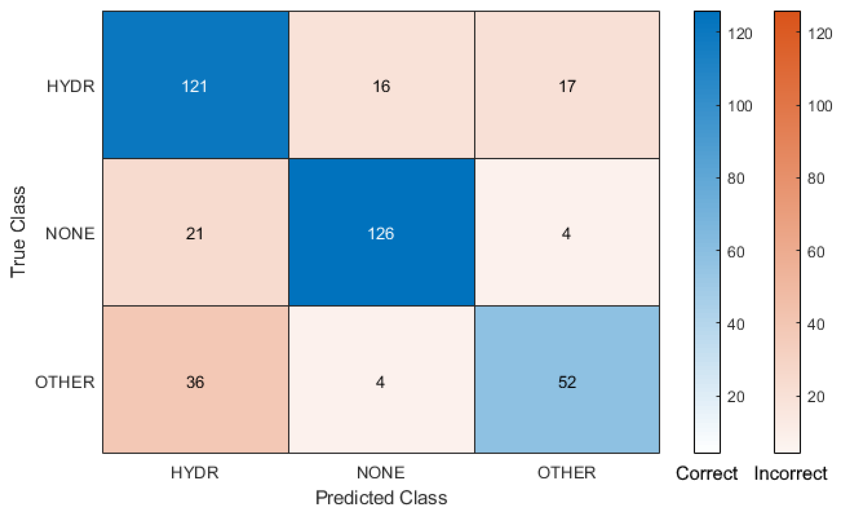
Classification performance was evaluated for the hydroacoustic and RGB ResNets and each of the different fusion methodologies. Figure 5 shows the confusion matrix resulting from initial training of the ResNet on hydroacoustic imagery. While the network achieves overall test set accuracy of 86%, it exhibits an obvious bias towards the “OTHER” class, largely due to class imbalances in the dataset. Moreover, the network exhibits obvious difficulty distinguishing between instances of hydrilla and other subaquatic species. This is illustrated by the poor recall score of 54.4% percent for hydrilla, and the precision score of 78.7%. However, in the limited test data, the network exhibits strong discriminatory performance between images with presence of SAV and those with no SAV present. The network exhibits 72.7% recall, but crucially 94.1% precision for the “NONE” class. These results fall in line with the expected. Hydroacoustic imagery is excellent at detecting the presence of submerged objects but gives relatively low image resolution, making detection of distinguishing features between species difficult.

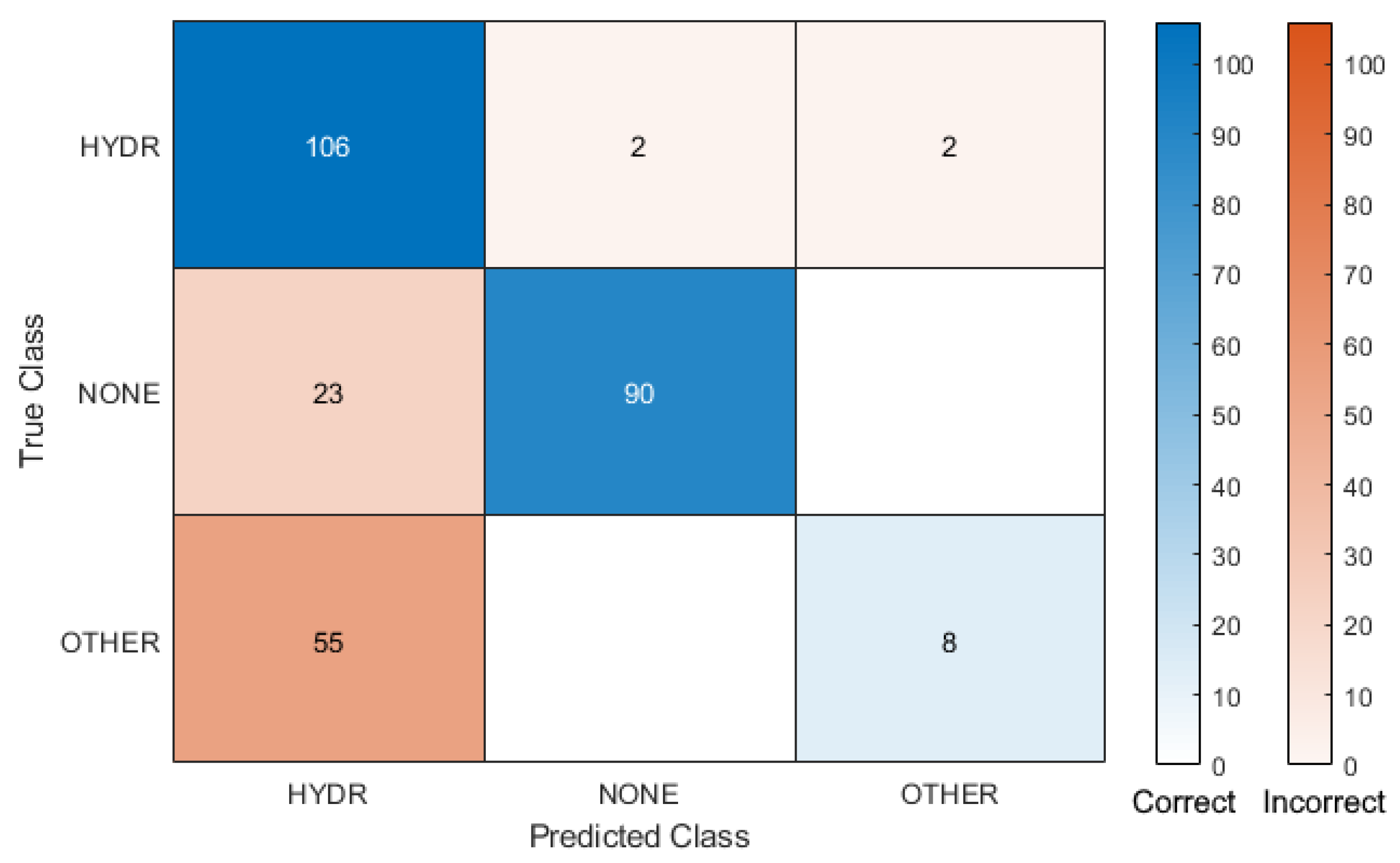
Figure 6 shows the confusion matrix generated on test data from a ResNet trained on aerial RGB imagery. The network achieves overall test accuracy of 75%, significantly worse than the performance seen when utilizing the hydroacoustic imagery. However, crucial to overall performance is the relative distribution of error between classes and the individual precision and recall scores. The network achieves 78.6% recall for hydrilla, meaning that it correctly identified 78.6% of the test images labeled as hydrilla, as compared to 54.4% recall for hydrilla when utilizing hydroacoustic data. Once again, these results fall in line with the expected. The relatively high resolution of aerial RGB pictures allows for identification of SAV near the top of the water column. Misclassifications between images labeled as “HYDR” and those labeled none occur when the turbidity of the water prevents SAV from being visually present in aerial images.

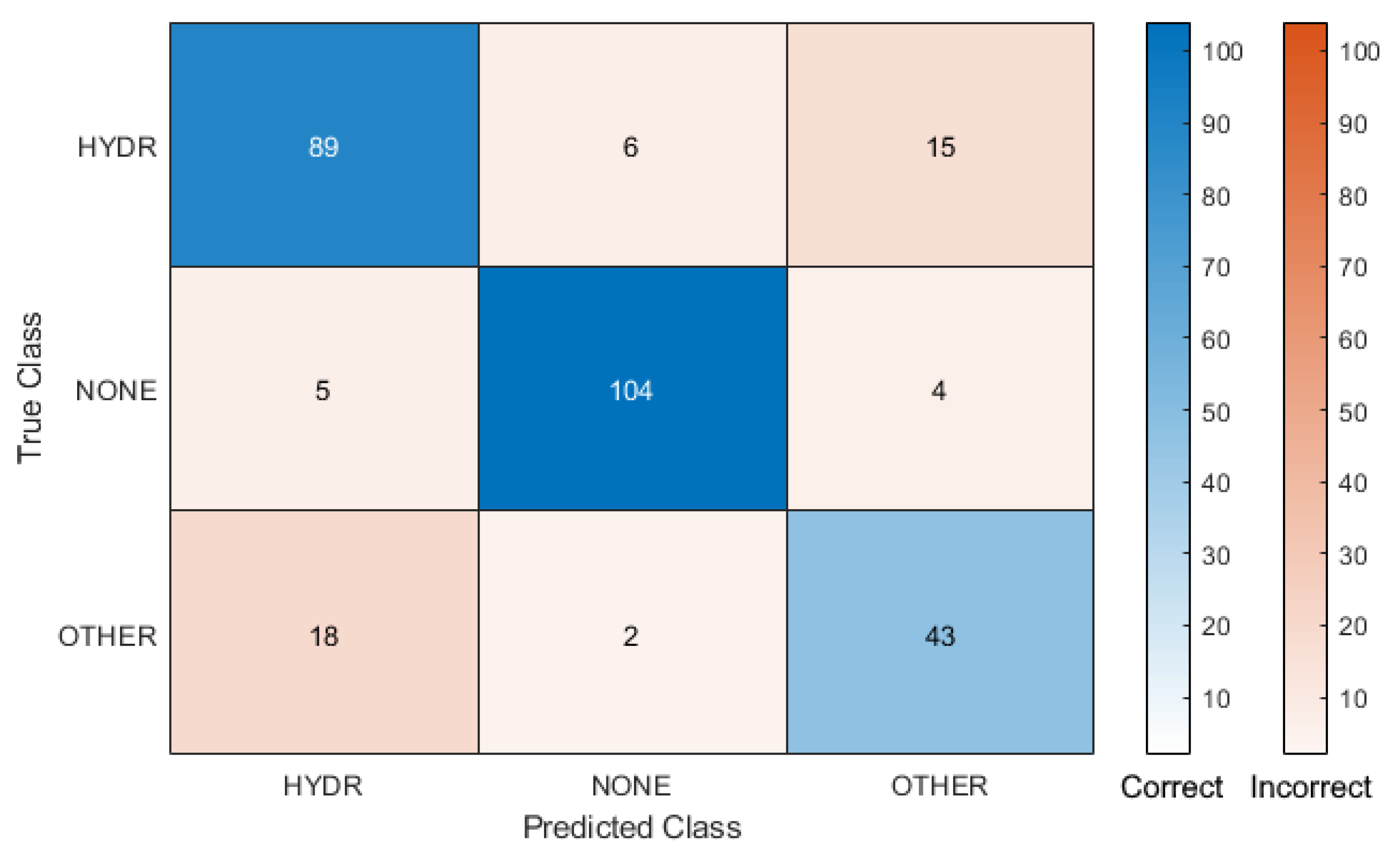
Figure 7 shows the confusion matrix generated by a simple, average-type bagging ensemble of the aerial RGB and hydroacoustic imagery. The ensemble has excellent recall performance for instances of hydrilla, but otherwise performs poorly in terms of precision. Moreover, the network performs poorly in terms of recall for both the “NONE” and “OTHER” classes. Examination of the test set confusion matrix for the hydroacoustic imagery alone reveals the tendency to predict any image with the presence of SAV as “HYDR”, hence the tendency in an average-based prediction model to overpredict instances of “HYDR.”

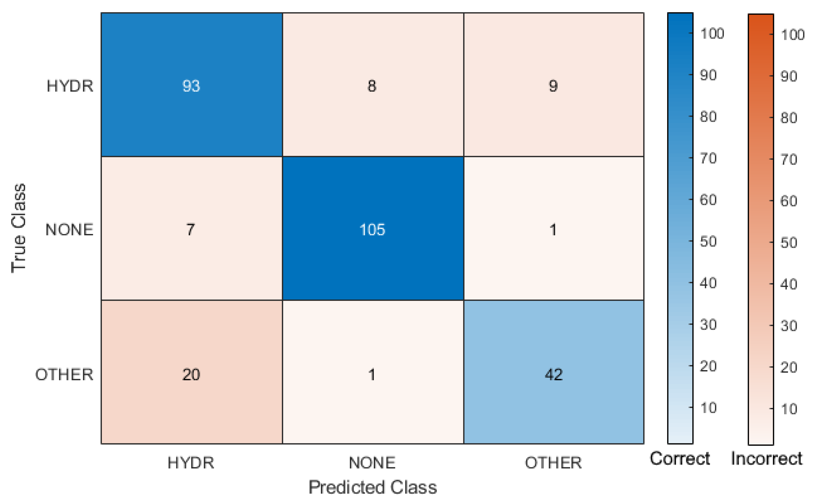
Figure 8 shows the confusion matrix generated by log-inverse uncertainty weighting for predictions generated by an MC Dropout type network. Results are nearly identical to those generated by the simple average ensemble. Again, the tendency of the hydroacoustic-based pipeline to confidently overpredict instances of the “HYDR” class results in an ensemble that, based on a weighted average, tends to overpredict “HYDR.”

Finally, Figure 9 and Figure 10 show the result of a logic-based approach to ensembling the two image types. The pure logic ensemble utilizes the vertical profile of the water column and robustness to turbidity of hydroacoustic imagery to accurately predict the presence or absence of SAV through the “NONE” classification. If SAV is detected through the hydroacoustic image, aerial RGB imagery is utilized to classify the present species as either “HYDR” or “OTHER.” The logic/MC combination follows the same procedure but applies the Monte Carlo dropout approach to predictions before applying the logical procedure. Both logic-based approaches vastly outperformed the weighted averaging approaches presented earlier, with overall test set classification accuracy reaching 84% for the logic/MC approach. In addition, precision and recall performance were generally improved across all classes (

Table 1. Precision/recall and overall accuracy for each of the approaches.

		HYDR	NONE	OTHER	Overall Accuracy
Hydroacoustic ResNet	Recall	54.4%	72.7%	96.0%	86.2% *
	Precision	78.7%	94.1%	87.0%
RGB ResNet	Recall	78.6%	83.4%	56.5%	75.3%
	Precision	68.0%	86.3%	71.2%
Average Ensemble	Recall	97.3%	82.3%	12.7%	72.7%
	Precision	58.8%	98.9%	80.0%
MC Dropout	Recall	96.4%	79.6%	12.7%	71.3%
	Precision	57.6%	97.8%	80.0%
Logic Ensemble	Recall	80.9%	92.0%	68.3%	82.5%
	Precision	79.5%	92.9%	69.4%
Logic/MC Ensemble	Recall	84.5%	92.9%	66.7%	83.9%
	Precision	77.5%	92.1%	80.8%

* Despite high overall accuracy, note the disparity in recall between HYDR and OTHER, due to oversampling of the OTHER class.

).

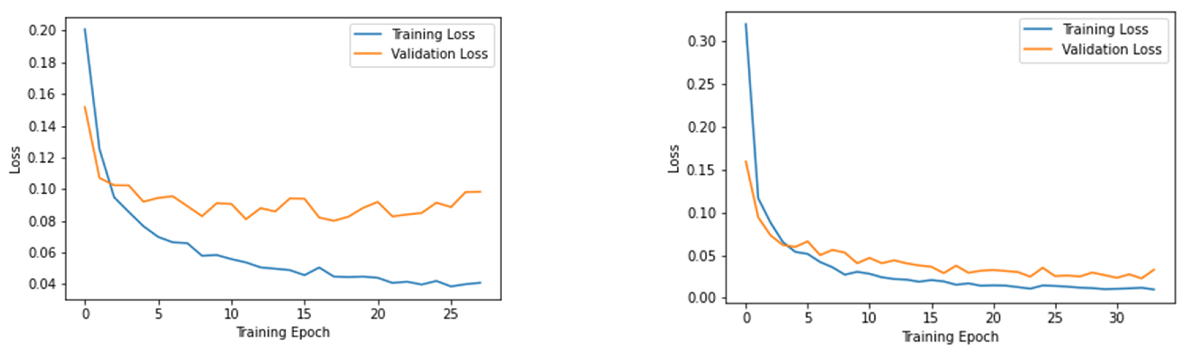
To assess performance with another network architecture, network training and testing were repeated for the six approaches above with the DenseNet model. Identical training and test datasets and methods were used for both the ResNet and DenseNet models. The DenseNet architecture yielded lower or nearly equal (within 0.3%) overall accuracy for all but the average ensemble approach (DenseNet average overall accuracy 69.0% vs. 70.9% for ResNet). In five out of six approaches, the DenseNet model produced lower classifications of HYDR (average 14.6% fewer) and higher classifications of NONE (average 8.3% higher) and OTHER (average 16.3% higher) compared to the ResNet model.

4. Discussion and Conclusions

Results indicate that sensor fusion can improve the automated classification of SAV relative to the performance provided by each of the individual sensing modalities. Acoustic imaging provided high precision in detecting the absence of SAV at all depths (NONE class), while neural networks trained on RGB images better distinguished hydrilla from other SAV. When ensembling outputs from the two modalities, applying logic provided the most notable improvement in classification accuracy. While not tested for statistical significance, combining the MC Dropout approach with logic provided a slight improvement to overall accuracy.

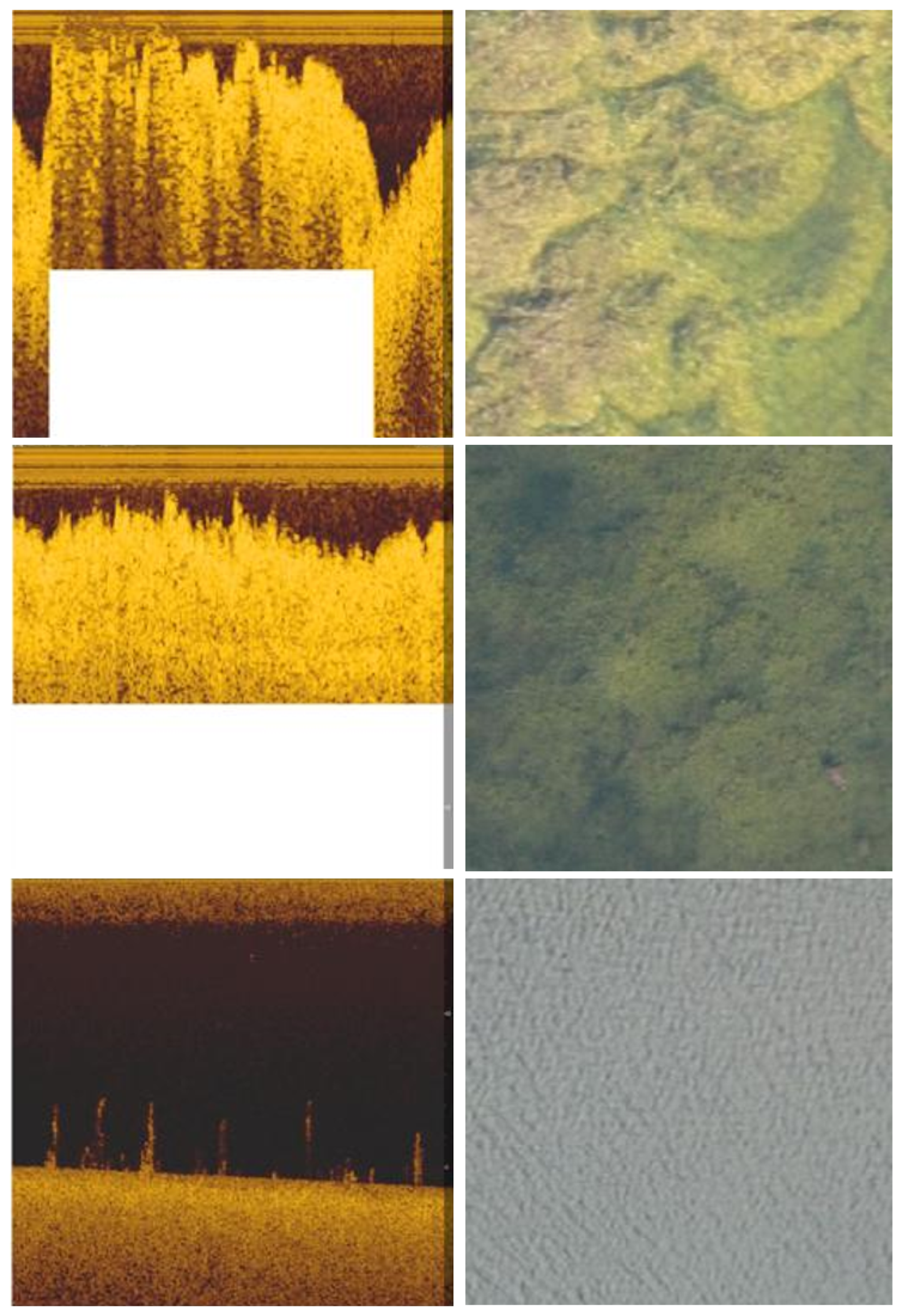
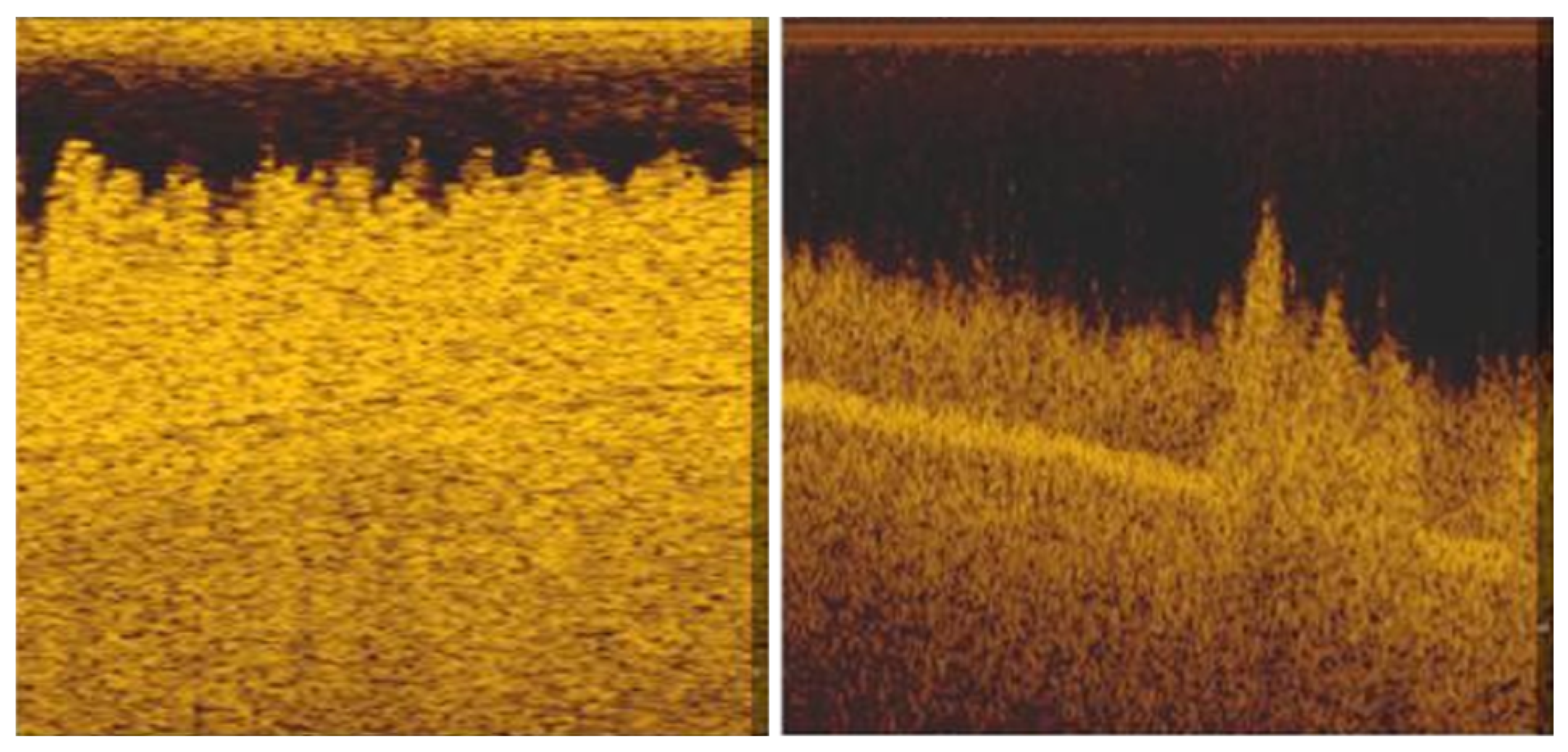
One area of particular interest was the tendency of the hydroacoustic imagery to overpredict instances of the “HYDR” class in test set data. Figure 11 shows representative images selected from the training data for the “HYDR” class images and test data selected from the “OTHER” class images.

In both images, the lake bottom is visually distinguishable, as well as vertical growth of bands of SAV beginning at the lake bottom. Due to the image resolution of hydroacoustic imagery and lack of color information available, little information is present in either image that can be used to distinguish between each species. Because of this, it is plausible that the hydroacoustic network learns to classify images fitting the form described above as “HYDR,” leading to frequent misclassifications. Aerial RGB imagery helps to remedy the lack of identifying information present in hydroacoustic images due to its much higher pixel resolution and the presence of color, shape, and depth information present in the feature-rich RGB spectrum. The result of the fusion of information is a network that is able to robustly detect the presence or absence of SAV across the range of water column heights, while also providing relatively high-accuracy classification of SAV near the top of the water column. However, there exists a range in the water column where classification accuracy performs poorly. When factors such as lake depth, turbidity, sun glint, wave action, and plant height render the SAV difficult to view from aerial imagery, hydroacoustic data are able to effectively identify the presence of SAV but often fail to distinguish between species. 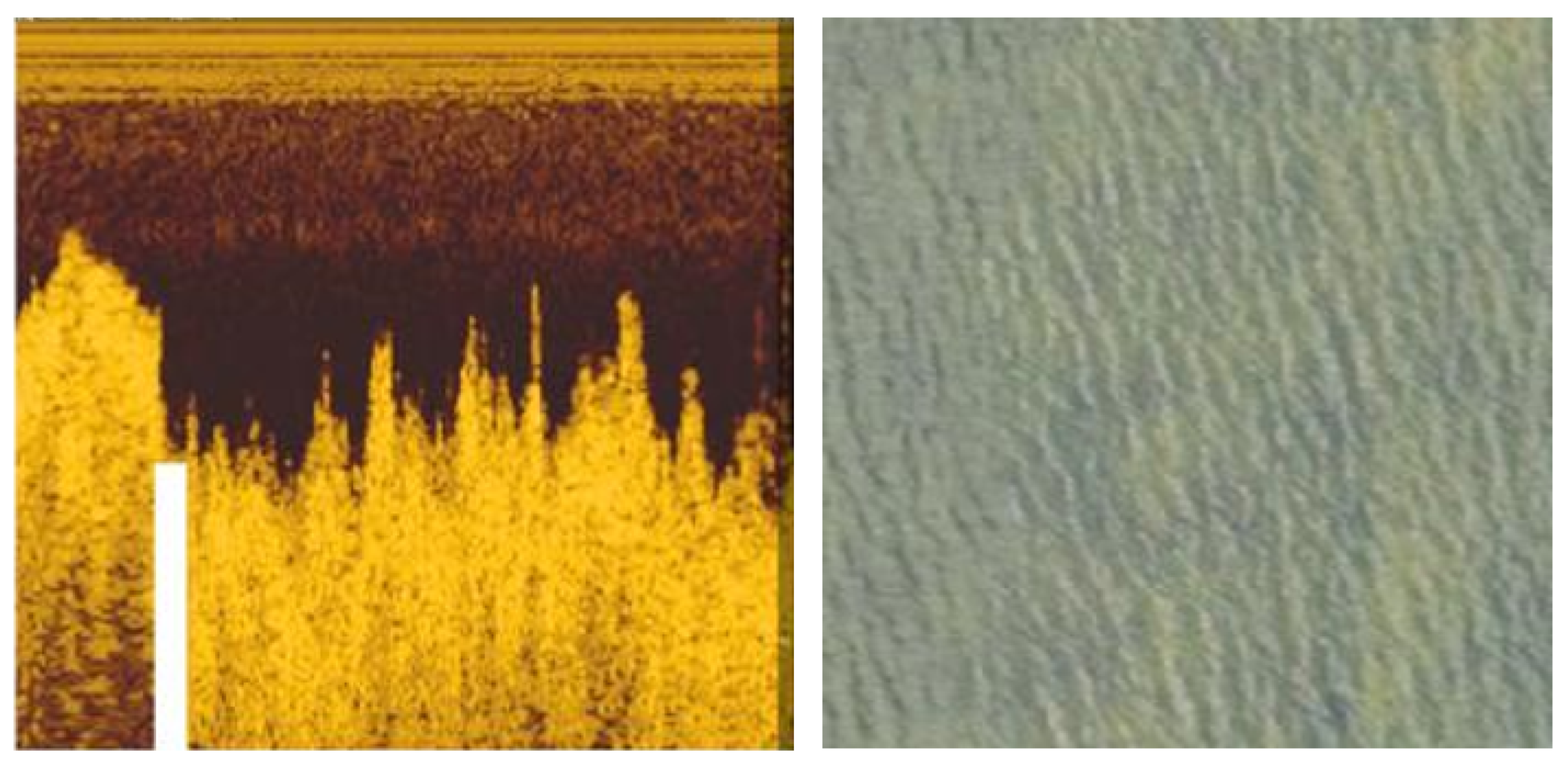Figure 12 shows an example of test set misclassification, where SAV obscured partially by wave action and plant depth is identified but misclassified.

Clearly, the growth of hydrilla is still present in the aerial RGB image. However, the features of the hydrilla growth used by the RGB-based neural network to perform classification are distorted as light passes through the water column. Consequently, the combined network is unable to consistently generate the correct classification of “HYDR” for the image pair shown.

While current classification performance still leaves room for improvement, the multi-sensor fusion approach for classification of subaquatic plant species demonstrates the potential to increase generalization and improve classification performance. Current fusion of aerial RGB imagery and hydroacoustic imagery exhibits classification performance that decreases as a function of increasing water turbidity and plant depth within the water column. However, all sensor data required for classification performance (hydroacoustic and RGB) are currently collected during a typical mapping operation. Addition of a third sensor, such as high-definition RGB images taken below the water surface, could provide the supplementary information needed to provide accurate classification in deeper water outside of the littoral zones. Alternatively, utilization of hydroacoustic systems with higher-definition imaging capabilities could potentially provide the same benefits, while maintaining the same runtime computational complexity and data collection burdens.

At the time of this publication, real-time classification utilizing the sensor fusion concept of this paper is currently under development. This methodology utilizes a Windows laptop running MATLAB and Python scripts, for data processing and classification, and a wireless SD card (Toshiba FlashAir, Toshiba, Tokyo, Japan) to transmit sonar log data from the sonar head unit to the laptop. UAV-based RGB images are captured asynchronously, prior to classification, and copied to the laptop hard drive. Tests to date indicate that sonar data collection and processing and sensor fusion classification can be performed in real time; however, transmission of sonar log data via the wireless SD card is currently inconsistent.

References

1. Cybenko, G. Approximation by superpositions of a sigmoidal function. Math. Control Signals Syst. 1989, 2, 303–314. [Google Scholar] [CrossRef]
2. Krizhevsky, A.; Sutskever, I.; Hinton, G.E. Imagenet classification with deep convolutional neural networks. Adv. Neural Inf. Process. Syst. 2012, 5, 1106–1114. [Google Scholar] [CrossRef]
3. Szegedy, C.; Liu, W.; Jia, Y.; Sermanet, P.; Reed, S.; Anguelov, D.; Erhan, D.; Vanhoucke, V.; Rabinovich, A. Going deeper with convolutions. In Proceedings of the IEEE Conference on Computer Vision and Pattern Recognition, Boston, MA, USA, 7–12 June 2015; pp. 1–9. [Google Scholar]
4. He, K.; Zhang, X.; Ren, S.; Sun, J. Deep residual learning for image recognition. In Proceedings of the IEEE Conference on Computer Vision and Pattern Recognition, Las Vegas, NV, USA, 26 June–1 July 2016; pp. 770–778. [Google Scholar]
5. Zhuang, F.; Qi, Z.; Duan, K.; Xi, D.; Zhu, Y.; Zhu, H.; Xiong, H.; He, Q. A comprehensive survey on transfer learning. Proc. IEEE 2020, 109, 43–76. [Google Scholar] [CrossRef]
6. Olsen, A.; Konovalov, D.A.; Philippa, B.; Ridd, P.; Wood, J.C.; Johns, J.; Banks, W.; Girgenti, B.; Kenny, O.; Whinney, J.; et al. DeepWeeds: A multiclass weed species image dataset for deep learning. Sci. Rep. 2019, 9, 2058. [Google Scholar] [CrossRef] [PubMed]
7. Rostami, M.; Kolouri, S.; Pilly, P.; McClelland, J. Generative continual concept learning. In Proceedings of the AAAI Conference on Artificial Intelligence, New York, NY, USA, 7–12 February 2020; Volume 34, pp. 5545–5552. [Google Scholar]
8. Jha, S.; Schiemer, M.; Zambonelli, F.; Ye, J. Continual learning in sensor-based human activity recognition: An empirical benchmark analysis. Inf. Sci. 2021, 575, 1–21. [Google Scholar] [CrossRef]
9. Ashfahani, A.; Pratama, M. Autonomous deep learning: Continual learning approach for dynamic environments. In Proceedings of the 2019 SIAM International Conference on Data Mining, Calgary, AB, Canada, 2–4 May 2019; Society for Industrial and Applied Mathematics: Philadelphia, PA, USA, 2019; pp. 666–674. [Google Scholar]
10. Li, D.; Liu, S.; Gao, F.; Sun, X. Continual learning classification method with new labeled data based on the artificial immune system. Appl. Soft Comput. 2020, 94, 106423. [Google Scholar] [CrossRef]
11. Patel, M.; Jernigan, S.; Richardson, R.; Ferguson, S.; Buckner, G. Autonomous robotics for identification and management of invasive aquatic plant species. Appl. Sci. 2019, 9, 2410. [Google Scholar] [CrossRef] [Green Version]
12. Houlahan, J.E.; Findlay, C.S. Effect of invasive plant species on temperate wetland plant diversity. Conserv. Biol. 2004, 18, 1132–1138. [Google Scholar] [CrossRef]
13. Gettys, L.A.; Haller, W.T.; Petty, D.G. Biology and control of aquatic plants. In A Best Management Practices Handbook: Third Edition; Aquatic Ecosystem Restoration Foundation: Marietta, GA, USA, 2014. [Google Scholar]
14. Pimentel, D.; Zuniga, R.; Morrison, D. Update on the environmental and economic costs associated with alien-invasive species in the United States. Ecol. Econ. 2005, 52, 273–288. [Google Scholar] [CrossRef]
15. Madsen, J.D. Point intercept and line intercept methods for aquatic plant management. APCRP Technical Notes Collection (TN APCRP-M1-02). U.S. Army Engineer Research and Development Center, Vicksburg, MS. 1999. Available online: https://apps.dtic.mil/sti/citations/ADA361270 (accessed on 27 April 2022).
16. Hauxwell, J.; Knight, S.; Wagner, K.; Mikulyuk, A.; Nault, M.; Porzky, M.; Chase, S. Recommended Baseline Monitoring of Aquatic Plants in Wisconsin: Sampling Design, Field and Laboratory Procedures, Data Entry and Analysis, and Applications; PUB SS-1068; Wisconsin Department of Natural Resources: Madison, WI, USA, 2010. [Google Scholar]
17. Lin, T.Y.; Goyal, P.; Girshick, R.; He, K.; Dollár, P. Focal loss for dense object detection. In Proceedings of the IEEE International Conference on Computer Vision, Venice, Italy, 22–29 October 2017; pp. 2980–2988. [Google Scholar]
18. Ganaie, M.A.; Hu, M. Ensemble deep learning: A review. arXiv 2021, arXiv:2104.02395. [Google Scholar]
19. Gal, Y.; Ghahramani, Z. Dropout as a bayesian approximation: Representing model uncertainty in deep learning. In Proceedings of the International Conference on Machine Learning, New York City, NY, USA, 19–24 June 2016; pp. 1050–1059. [Google Scholar]
20. Laakom, F.; Raitoharju, J.; Iosifidis, A.; Nikkanen, J.; Gabbouj, M. Monte Carlo Dropout Ensembles for Robust Illumination Estimation. In Proceedings of the 2021 International Joint Conference on Neural Networks (IJCNN), Shenzhen, China, 18–22 July 2021; IEEE: Piscataway, NJ, USA, 2021; pp. 1–7. [Google Scholar]
Figure 1. Autonomous aquatic drone designed and fabricated for identification of invasive aquatic plant species (left); example hydroacoustic image of hydrilla (center); deep learning classification accuracy as a function of training iterations (right). From Patel et al., 2019 [11].
Robotics 11 00068 g001
Figure 2. Orthomosaic of Lake Mann (Orange County, FL, USA) at 3 cm ground sampling distance (GSD), acquired on 9 February 2021.
Robotics 11 00068 g002
Figure 3. Loss curves for ResNet training of RGB images (left) and hydroacoustic images (right).
Robotics 11 00068 g003
Figure 4. Top: RGB and hydroacoustic images of hydrilla at the top of the water column. Middle: hydrilla in the middle of the water column. Bottom: no SAV present. Note: solid white areas in hydroacoustic images represent regions in which hydroacoustic data are not present due to automatic depth ranging of the sonar unit.
Robotics 11 00068 g004
Figure 5. Hydroacoustic ResNet confusion matrix for test images.
Robotics 11 00068 g005
Figure 6. RGB ResNet confusion matrix for test images.
Robotics 11 00068 g006
Figure 7. Average ensemble confusion matrix for test images.
Robotics 11 00068 g007
Figure 8. MC Dropout confusion matrix for test images.
Robotics 11 00068 g008
Figure 9. Logic ensemble confusion matrix for test images.
Robotics 11 00068 g009
Figure 10. Logic/MC ensemble confusion matrix for test images.
Robotics 11 00068 g010
Figure 11. Left: HYDR training image. Right: OTHER test image.
Robotics 11 00068 g011
Figure 12. Left: Hydroacoustic image of misclassified test set. Right: RGB image of same test point.
Robotics 11 00068 g012