Article

Elasto-Geometrical Model-Based Control of Industrial Manipulators Using Force Feedback: Application to Incremental Sheet Forming

LGCGM, INSA Rennes, University of Rennes, 20 Avenue des Buttes de Cöesmes, CEDEX, 35043 Rennes, France
*
Author to whom correspondence should be addressed.
Robotics 2022, 11(2), 48; https://doi.org/10.3390/robotics11020048
Submission received: 18 February 2022 / Revised: 30 March 2022 / Accepted: 7 April 2022 / Published: 12 April 2022
(This article belongs to the Special Issue Industrial Robotics in Industry 4.0)

Abstract

:
This paper aims to improve the positioning accuracy of serial industrial manipulators using force feedback in manufacturing processes by implementing an elasto-geometrical model-based control. Initially, the real-time position control strategy using a force feedback to elastically correct the Tool Center Point (TCP) pose of serial industrial manipulators is detailed. To continue, an efficient model structure identification and calibration is proposed to shorten the elasto-geometrical modeling process. The Virtual Joint Method (VJM) is chosen to iterate and complete the robot stiffness modeling. This method considers that the elastic deformations are only localized at the joints of the robot. An appropriate and original test-model approach allows a minimum of optimization iterations to find the best compromise between complexity and accuracy of the modeling. The proposed approach is illustrated in detail by the Stäubli TX200 robot modeling. Finally, the reliability and responsiveness of the developed control framework is then evaluated through experimental tests in an Incremental Sheet Forming (ISF) context. An average improvement of 70% in trajectory-tracking accuracy is achieved during these tests. Overall, the high accuracy and responsiveness of the developed system demonstrate a promising potential for deploying industrial manipulators to a cost-effective manufacturing processes in industry 4.0 .

Graphical Abstract

1. Introduction

Current research in manufacturing processes for Industry 4.0 is enhancing Computer-Aided Manufacturing (CAM) techniques to lower the environmental, human time and investment cost of producing a good-quality part [1]. For this purpose, the research field is transitioning from relying exclusively on traditional CNC machines toward using much more versatile and affordable industrial manipulators. In process conditions (e.g., Friction Stir Welding (FSW), Incremental Sheet Forming (ISF), machining or any robotic manufacturing process), the interaction between the tool and its environment brings up the challenge of accurate robot positioning. Indeed, the trajectory of the tool during CAM has to be precisely and accurately controlled to produce the desired part from its Computer-Aided Design (CAD) model. When a given wrench is applied on the tool, the elastic deformation of the machine lowers the global positioning accuracy, especially for industrial serial manipulators undergoing high process loads.
To cope with external wrenches and compensate for the elastic deformation of a robot, several methods are used, each suited to different industrial applications:
  • Robot category upgrade;
  • Absolute pose feedback control;
  • Force control;
  • Model-based compensation.
The first method is to directly change the machine used to overdesign its stiffness characteristics. By upgrading the category of the robot with regard to its payload capacity, the elastic deformation will decrease for the same range of wrenches applied [2].
The second method is to implement an absolute position feedback control, usually relying on external sensors [3,4,5]. Most commonly, the tool is tracked by an exteroceptive sensor (for instance, a laser tracker [6], an encoder [7] or a 3D camera [8,9]), and the position feedback enables real-time compensation for the robot’s inaccuracy. This method achieves up to a 70% accuracy improvement by using a laser tracker with heavy-duty robots [6]. Another use of position feedback is to perform deformation-tracking impedance control coupled with an Extended Kalman Filter [10]. Other research studies use proprioceptive sensors such as double encoders on each joint to measure the angular displacement before and after the motorized body [11,12]. This technique only compensates for the elasticity of the actuated joints and implies a specific robotic design to integrate the second encoder on each joint.
The third method is a force control loop which uses the common force sensor present in most robots to actively control the output force applied by the tool in one or multiple directions [13]. For specific cases such as FSW, this can help stabilize the process and increase its reliability [14]. However, this method only works for hybrid control scenarios when a given DoF is force-controlled, while the environment constrains its position [15,16]. More generally, without a force input, the present study takes the wrench applied on the tool as an environmental constraint with its effect to be compensated.
The fourth method is a model-based compensation, where prior knowledge of the machine’s behavior is needed. Although a geometrical calibration of a loaded robot can virtually correct those imperfections by adding extra geometrical parameters or modifying existing ones [17,18,19,20,21,22], it does not correspond to the physical behavior of the manipulator. Indeed, there is no proportionality between the force input and the deformation of the machine, so it is only valid for a constant load scenario. To better describe the machine’s behavior, an elasto-geometrical model is needed to proportionally link the deformation of the robot with the applied wrench. This type of model needs a calibration phase by applying external wrenches and measuring the resulting elastic deformations [23].
To estimate the deformation of a machine due to an external wrench applied on its End Effector (EE), the three main modeling approaches are Finite Element Analysis (FEA), Matrix Structural Analysis (MSA) and the Virtual Joint Method (VJM).
  • Currently, FEA models are the most accurate since they model each point of the machine with a high resolution. However, they require a significant amount of calculation time as well as parameters often only accessible by the manufacturer during the design phase of the structure [24,25].
  • MSA models are based on the Euler–Bernoulli beam theory. They are well-suited for simple and slender geometrical structures used for parallel manipulators [26,27]. This method allows the description of the behavior of the joints using an appropriately located stiffness matrix setting up the radial, axial, radial rotational and axial rotational stiffnesses of each joint.
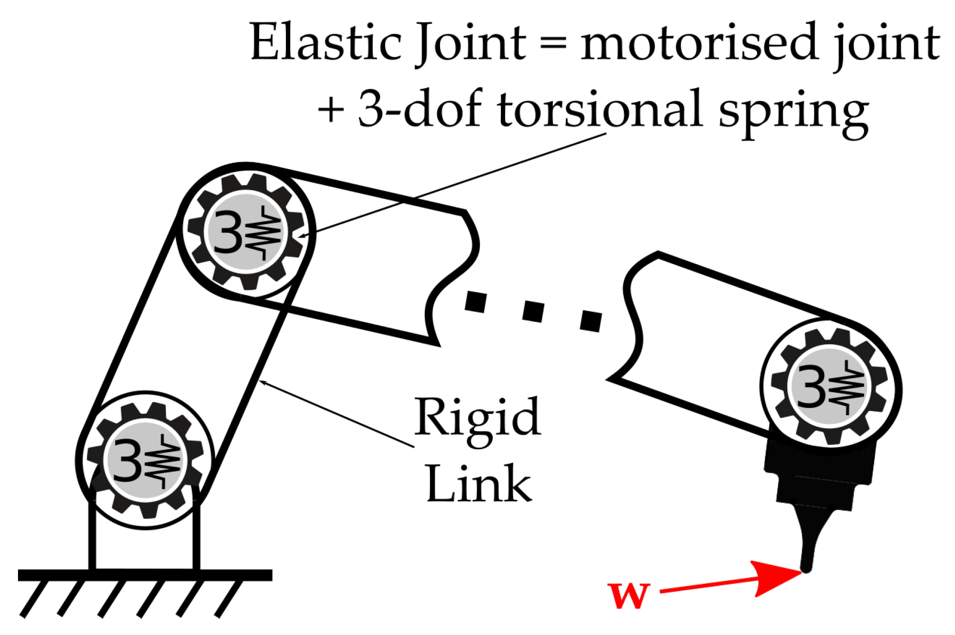
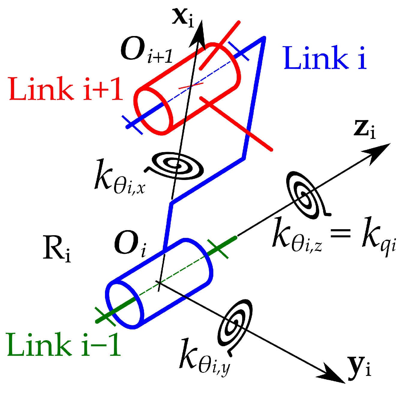
  • A special case of MSA is the VJM, also called lumped-stiffness modeling, where the elastic deformations are only localized at the joints [28]. Indeed, several research works have demonstrated that for industrial anthropomorphic robots, deflection errors are mainly due to joint elasticity [29]. Furthermore, for the sake of simplicity, the elasticity of each joint is usually modeled by a single torsional spring located along its motorized axis to integrate the elastic deformations of the structure, the joint and the actuator [30].
In the literature, two methods are traditionally used to identify the stiffness model parameters of a serial robot, either with a local axis-by-axis study or globally with a large set of measurement points in the robot workspace [29]. The first method consists of studying the independent elastic deformation of one joint for a known wrench to measure its independent stiffness. This variable links the angular displacement with the torque applied, and the procedure is repeated for each revolute joint [31]. The second method measures the tool cartesian displacement due to an external wrench on a large set of points before performing a root-mean-square regression to extract the stiffness values [32]. Either unpractical in real environment or too long to achieve, both methods also predefine the structure of the model which stays constant throughout the whole calibration process. Then, for correcting the trajectory based on the stiffness modeling, the machine’s deformation can be computed offline from a wrench prediction [33,34,35,36]. If the external wrenches cannot be predicted, an online force sensor is implemented [14,37].
The main objective of this article is to tackle the issue of low positioning accuracy of industrial manipulators due to their elastic deformation in processes involving interaction of the tool with its environment. The proposed methodology is based on three key features. The main contribution of this article is the practical implementation of those key features combined for the ISF process:
  • The first feature is the development of an efficient test-model approach to identify the model structure and calibrate the elastic parameters of an industrial serial robot. Using rigorous iterations, the elasto-geometrical model is identified and enhanced, aiming at the best compromise between complexity and accuracy before being validated during experimental tests.
  • The second feature is the implementation of an elasto-geometrical model-based position control loop with force feedback to elastically correct the Tool Center Point (TCP) pose of any serial robot.
  • The third feature is the validation of both the identification approach and the elastic correction strategy on a real ISF application.
The overall structure of this article follows the different steps of the research process. Firstly, the real-time control strategy of the industrial manipulator and its elastic correction are presented. Secondly, the identification of the robot elasto-geometrical model and its results are described. Thirdly, the control strategy is validated during several ISF process experiments using the Stäubli TX200 industrial robot. Finally, the last section presents results and discusses directions for future works.

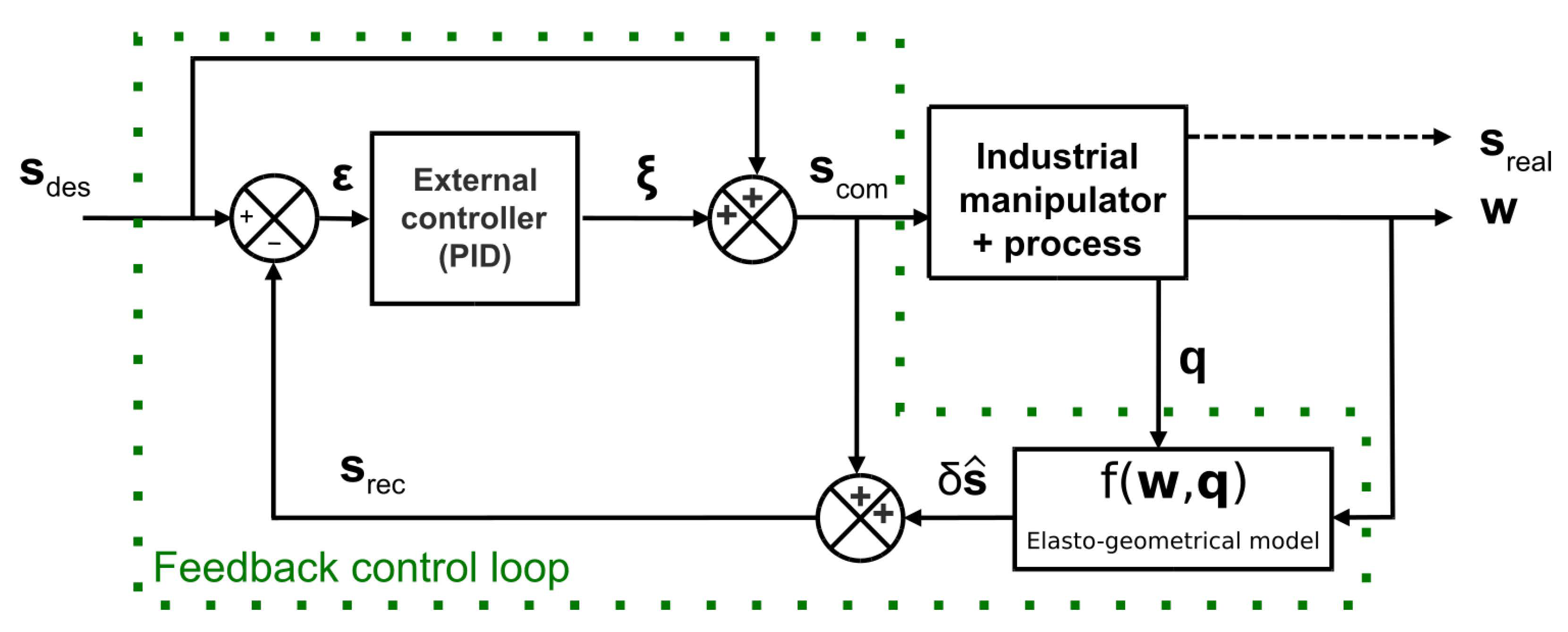
2. Force-Feedback Position Control Based on Elasto-Geometrical Modeling

In the following section, a model-based position control strategy of industrial manipulators is presented along the elasto-geometrical model on which it is based.

2.1. Position Control Strategy of Industrial Manipulators Using a Force-Feedback Loop

As presented in Figure 1, a model-based position control strategy with a force-feedback loop is depicted for industrial manipulators. To describe the motion of a serial industrial manipulator subject to an environmental wrench w , the robot structure is considered as a series of joints and links with the following attached frames:
  • R 0 = ( O 0 , x 0 , y 0 , z 0 ) is the base frame of the robot;
  • R t = ( O t , x t , y t , z t ) 
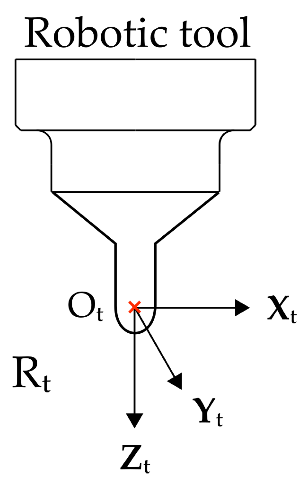
is the robot tool frame.
The point of interest is the TCP, the R t -frame origin O t at the center of the hemispherical tip of the tool (Figure 2). In the following equations, all vectors are expressed in the base frame R 0 if not specifically stated. The desired cartesian pose of O t is:
s d e s = 0 s t = 0 p t 0 ϕ t = g ( q ) ,
where 0 p t = p x , p y , p z T represents the desired position vector and 0 ϕ t = ϕ x , ϕ y , ϕ z T the desired orientation vector of the tool frame R t ; s d e s is a function of the articular configuration q = q 1 q m T of the robot.
Let w be the wrench applied by the environment on the robot tool:
w = [ f x f y f z m x m y m z ] T .
Considering a rigid robot, this desired pose is sent and reached by the manipulator (configuration (a) in Figure 3).
In reality, an industrial manipulator presents an elastic deflection δ s measurable at the TCP, depending on the articular configuration q and the external wrench w :
δ s = 0 δ s t = 0 δ p t 0 δ ϕ t = f ( w , q ) ,
where 0 δ p t = δ p x δ p y δ p z T represents the position deflection vector of the TCP and 0 δ ϕ t = δ ϕ x δ ϕ y δ ϕ z T represents the angular deflection vector of the tool frame R t .
Therefore, the pose effectively reached by the TCP of the robot is s r e a l (configuration (b) in Figure 3), which can be computed as follows:
s r e a l = s d e s + δ s .
The presented control strategy estimates the elastic deflection δ s ^ by means of an elasto-geometrical model using the external wrench information w measured by a 6D force sensor mounted on the robot tool (Figure 1). This model-based reconstruction, described in Section 2.2, avoids the use of an absolute pose measurement system.
The closed-loop dynamics are defined by the tracking error equation:
ε = s d e s s ^ r e a l ,
with
s ^ r e a l = s c o m + δ s ^ .
s c o m is the corrected pose, the new setpoint fed to the robot controller, and s ^ r e a l is the reconstructed pose vector of the robot, estimation of its real position s r e a l under load. Finally, the corrected pose s c o m is expressed as follows:
s c o m = s d e s + ξ ,
where ξ corresponds to the pose correction vector defined as a function of the tracking error ε and the external control law parameters (proportional, derivative and integrator gains in case of a PID controller).

2.2. Elasto-Geometrical Modeling

The elasto-geometrical model developed to be used for elastic deflection estimation of a robot under external load is based on the VJM approach. In this paper, the hypothesis taken is that the elasticity of the manipulator solely resides in its elastic joints [24,28,29,38,39]. The result is a model of the robot as a series of nondeformable rigid links and flexible joints. A focus is made on modeling the elastic deformations of a robot undergoing an external wrench applied on its tool (Figure 4). By generalizing the term of elastic Degree of Freedom (eDoF), the lumped-stiffness identification method proposed in this paper allows us to obtain a scalable model with the aim of staying as close as possible to the physical behavior.
Let us consider an industrial serial manipulator with m motorized joints (hereafter named mDoF) and m + 1 rigid links. In addition to R 0 and R t defined previously, a local frame R i = ( O i , x i , y i , z i ) is defined, attached to the i t h rigid link ( i [ 1 , m ] ). Joint i connects links i 1 and i (Figure 5). It is to be noted that for elastic modeling purposes, the origin O i of coordinate frame R i is not necessarily located at the intersection point of the z i 1 - z i common normal and the joint i axis, as defined by the modified Denavit–Hartenberg (mDH) convention. While being placed on the joint i axis to respect the kinematic constraints, the modification of the placement of the center of the joint does not guarantee a minimal representation but allows us to have a representation as close as possible to the real features of the physical structure.
To deal with the full elasticity of each joint, the VJM approach is generalized by considering two complementary rotational eDoFs for each joint (Figure 5). Two additional torsional springs are then defined around axes orthogonal to the joint axis z i of each local frame R i , thus completing the usual one-eDoF-per-joint elastic model [25,28,29,30,40,41].
In the absence of coupling terms and for slow motions, the reaction torque τ i , j around the axis j { x , y , z } of joint i [ 1 , m ] is taken as a function of the rotational stiffness coefficient k θ i , j and the rotational elastic displacement δ θ i , j associated to that eDoF [42,43]:
τ i , j = k θ i , j δ θ i , j i , j .
The elastic displacement vector of the robot δ θ is defined as the concatenation of the small rotational displacements associated to all virtual eDoFs i , j :
δ θ = δ θ 1 , x δ θ i , j δ θ m , z T .
Generalized to the whole structure, the torque vector τ can then be expressed according to the articular stiffness matrix K θ and the angular displacement vector δ θ :
τ = K θ δ θ ,
where K θ is the articular stiffness matrix gathering all torsional stiffness parameters (each being associated to a specific eDoF). By neglecting the coupling terms between directions, K θ is considered diagonal:
K θ = d i a g ( k θ 1 , x k θ i , j k θ m , z ) .
For a given articular configuration, the relationship between the small rotational elastic displacements and the elastic displacements δ s at the TCP is expressed by means of the Jacobian matrix J as follows:
δ s = J δ θ ,
where the Jacobian matrix J is defined as:
J = x 1 × O 1 O t v i , j × O i O t z m × O m O t x 1 v i , j z m .
where v i , j is the vector associated with the considered eDoF i , j expressed in the robot base frame (so 0 x i , 0 y i or 0 z i ), and × denotes the screw product.
Assuming low process speeds (under 1 m/min [14]), the mapping between the generated torque vector τ acting on the different virtual eDoFs and the external wrench w acting on the robot tool is represented by the following equations:
τ = J T w = τ 1 , x τ i , j τ m , z T .
By combining Equations (10), (12) and (14), one obtains the following equation:
δ s = J K θ 1 J T w .
Finally, by inserting Equation (15) into Equation (6), the reconstructed pose s ^ r e a l becomes:
s ^ r e a l = s d e s + ( J · K θ 1 · J T ) w + ξ .
In practice, not all stiffness parameters are needed to accurately model the behavior of the robot, depending on its architecture and dimensions. A trade-off between accuracy and complexity was researched to derive the best-fitting stiffness matrix K θ for the minimum number of eDoFs considered. Therefore, the effectiveness of the correction will depend on the number of these elasto-geometrical parameters and the quality of their calibration. A detailed example of the elasto-geometrical model identification is presented in Section 3.

3. Elasto-Geometrical Model Identification and Calibration

In this section, an efficient model structure identification and calibration is carried out. The robot elasto-geometrical model is identified and calibrated using an appropriate coupled test-model approach with the minimum number of measurement configurations (Figure 6). In this approach, the only hypothesis taken is the premise of the VJM approach: the elasticity of the robot is modeled only in its joints. To identify the joint torsional stiffnesses, the robot was placed in specific articular configurations where a given external wrench applied on the robot EE using a tension cable was able to generate a torque onto the minimum number of joint axes [31]. The different tests allowed a progressive enhancement of the model structure and an iterative calibration of the stiffness parameters to increase modeling accuracy, starting from a classical one-eDoF-per-joint configuration [28,38,39]. A compromise between complexity and accuracy is to be found to make it usable in a real industrial robotic application.

3.1. Refinement of the Elasto-Geometrical Model of the Stäubli TX200

The proposed elasto-geometrical model identification was implemented on the Stäubli TX200 robot, a 6-mDoF anthropomorphic serial robot with a payload capacity of 130 kg. It is to be noted that the robot was not symmetrical, the arm being offset with a U-shaped design (Figure 7). To identify and calibrate the elasto-geometrical model, the robot was loaded with a cable whose tension and direction could be manually controlled. An ATI Omega-160 6-DoF load cell was used to measure the wrench applied by the cable tension on the robot EE (point O E E ), and an API Radian laser tracker was used to measure the cartesian position of point O E E . In the following tests, the orientation was not measured nor used in the calibration of the model; nevertheless, the model estimated the full elastic deflection in position and orientation.
Let us first consider the specific configuration depicted in Figure 7. The robot articular configuration is q = 0 p i 2 0 0 0 0 T and the wrench applied on its EE were set to w = 0 f y 0 0 0 0 T with the maximum value being f y = 1400 N. It is noteworthy here that the first actuated joint was primarily solicited. It is, however, important to carefully examine the elastic behavior of the other joints of the robot. The global elastic response of the robot was evaluated based on the displacements of three points, M 1 , M 2 and M 3 , attached to the robot structure as shown in Figure 7 and measured with the API laser tracker. Figure 8 and Figure 9 show the displacements measured along the x 0 -axis and the y 0 -axis, respectively. As one can see, a significant displacement along the x 0 -axis can be observed, specifically at measurement points M 2 and M 3 . It is also important to observe the nonproportionality of the displacement along the y 0 -axis with respect to the distance of the measurement points from the center of the robot base frame O 1 . The experimental outcomes clearly illustrate that the robotic arm does not exhibit a simple rigid-body motion in rotation about the first actuated joint. There is a nonnegligible flexibility at the robot arm elbow.
Using a one-eDoF-per-joint model would result in a consequent error on the elastic model prediction along the x 0 -axis (Figure 8) and a physical misinterpretation of the experimental results in the y 0 direction (Figure 9). It is thus necessary to introduce an additional torsional stiffness on the third joint, while shifting the center O 3 of the joint along the z 3 -axis by 400 mm. The mDH parameter table associated to the kinematic chain of the robot arm was thus enhanced by an additional parameter δ r 3 describing this translation. The torsional joint stiffness value k θ 3 , x was evaluated from the EE displacement along the x 0 -axis, the robot geometric parameters and the force applied on it. After calibration of this stiffness parameter, the EE elastic displacement measured along the y 0 -axis allows the calibration of the torsional stiffness coefficient k θ 1 , z .
The complete model resulting from this identification process clearly improves the elastic displacement prediction compared to a one-eDoF-per-joint model (Figure 8 and Figure 9). It should be noted that in both models, the following displacement along the x 0 -axis measured at point M 1 is not perfectly predicted. Further experimental analysis in this configuration has shown that this displacement is due to the robot baseplate tilting around the y 0 -axis. This elastic effect is not taken into account in this study but could be added to improve accuracy in future works.
To complete the model structure identification and calibration of the TX200 elasto-geometrical model, four additional configurations are required (Table A1 and Table A2). Each specific articular configuration relates to a given wrench w with a gradual evolution of its components. The resulting independent torsional joint-stiffness parameters representing the physical stiffness elements of the actual structure are given in Table 1. A physically-representative elasto-geometrical model is then easily set up from the model structure identification and iterative axis-by-axis calibration process. It is important to note that the joint six stiffness is neglected in the proposed model as the wrist is not stressed around the z 6 -axis in the studied ISF application.

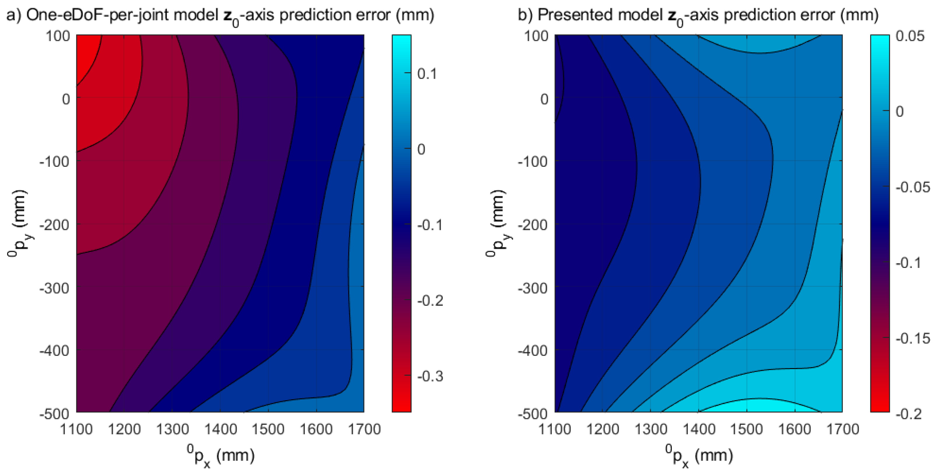
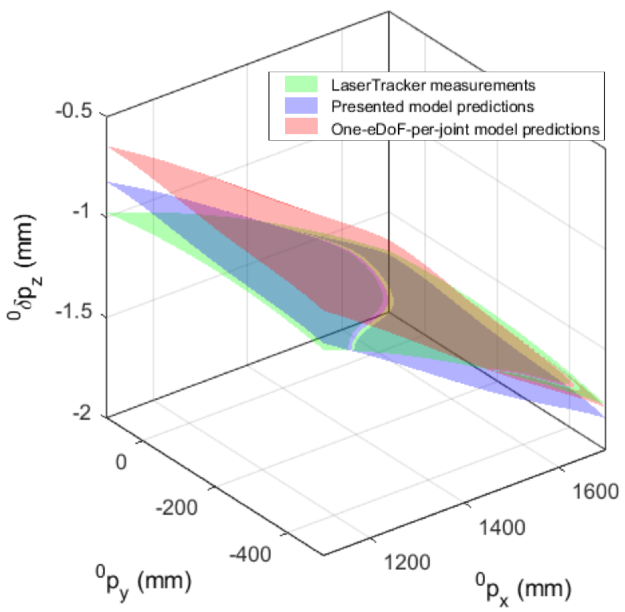
3.2. Validation of the TX200 Elasto-Geometrical Model

To verify the global elasto-geometrical model accuracy, the EE elastic displacements that this model allows us to predict were compared with those measured experimentally. This was accomplished by using two sets of measurements performed with loads of 600 N and 1100 N applied by the use of deadweights attached to the robot EE. The results are respectively shown on Figure 10 and Figure 11 for the 600 N case and on Figure 12 and Figure 13 for the 1100 N case. The accuracy of the position after calibration was tested on 200 poses regularly distributed over a 0.6 × 0.6 m ( 0 p z = 0.1 m) horizontal grid centered on the work area that was used for the ISF application (Section 4). Compared to the results obtained with the one-eDoF-per-joint elastic model, the proposed enhanced elasto-geometrical model allows for a better prediction of the EE vertical elastic displacements. By comparing the model predictions and the laser tracker measurements, the one-eDoF-per-joint elastic model gives a prediction of the elastic behavior with a maximum deviation of 0.18 and 0.34 mm and a RMS deviation of ± 0.16 and ± 0.11 mm over the studied workspace for the 600 and 1100 N loads, respectively (Figure 11a and Figure 13a). The addition of an extra eDof and the shifting of joint three origin allows better accuracy for loads of 600 and 1100 N. For the proposed model, the maximum error was 0.08 and 0.16 mm, and the RMS error was ± 0.04 and ± 0.05 mm over the same workspace for the 600 and 1100 N loads, respectively (Figure 11b and Figure 13b). The prediction accuracy of the proposed model is compatible with ISF requirements within a prototyping context [27].
A second validation of the elasto-geometrical model was made over a 0.25 -m-initial-radius spiral trajectory in which the robot EE was loaded with a 600 N deadweight-type force (Figure 14a). The continuous trajectory had a length of 2.7 m, the EE motion speed was 10 mm/s, and the raw laser tracking data were gathered at 50 Hz. The plane in which the spiral was located was 0.2 m above the working area used for the ISF application (Section 4), resulting in 0 p z = 0.3 m. As one can see in Figure 14b, the presented model confirms an accurate prediction of the elastic behavior over a given trajectory.

4. Application to Forming Processes: ISF Experiment

The performance and effectiveness of the proposed real-time force-feedback model-based control of industrial manipulators were evaluated and verified through some experimental tests in an ISF context. ISF is a cost effective die-less forming process for small batch production, traditionally used for customization or prototyping as an alternative to conventional stamping or deep drawing [44]. The material is incrementally pushed down by a simple tool, usually a hemispherical punch, to form the part step-by-step from its CAD model [45]. Many developments of the technology happened in the past 20 years [46], and the process can be used for several applications, for example to form parts in the medical and aviation sectors [36]. Recently, research trends are pushing toward a Robotized Incremental Sheet Forming (RISF) variant with the goal of enhancing the effective workspace, the dimensions of the manufactured parts and the versatility of the process [45]. The industrial manipulator is mounted with the forming tool on its flange to perform the desired forming trajectory. The main drawback of using such a machine is that the robot elastically deforms itself under the wrench generated by the process at the tool/sheet contact (Section 2.2) [33]. Hence, the tool trajectory stresses the robot structure in all directions all along the path. The level of forces induced by the process evolves along the trajectory and is multifactorial, making it difficult to predict [27]. The ISF process is therefore controlled by a TCP pose set-point.

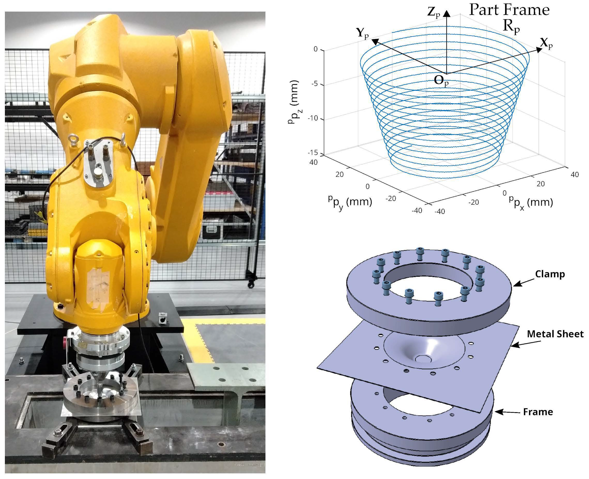
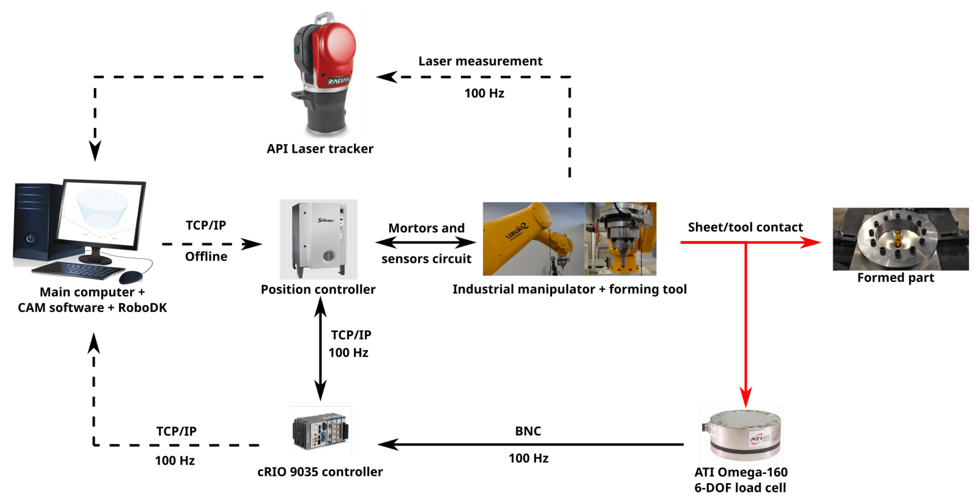
4.1. Experimental Setup

The Stäubli TX200 robot was used to form a 1-mm thickness metal sheet (Aluminium 5086 grade) with a forming tool which was a 15-mm diameter hemispheric punch blocked in rotation. The clamping system was composed of a circular blank holder screwed on a rigid frame (Figure 15). To ensure repeatability of the test, the formed metal sheets were placed in a similar manner with a fixed rolling direction and clamped with the same torque for all 12 screws.
The target toolpath was a 40-mm diameter frustum cone of 45° wall angle (Figure 15). The 3D complex path was defined in the part frame R p = ( O p , x p , y p , z p ) with O p of position coordinates [1500 0 183 ] T mm, expressed in the robot base frame. This central point of the trajectory corresponded to a robotic articular configuration of [ 0 49.7 89.3 0 41 0 ] T deg. Mineral oil was used as lubricant to avoid excessive friction at the tool/sheet contact.
This trajectory was firstly simulated using FEA following the procedure of [33]. Because of the continuous evolution of the z-coordinate along the frustum cone trajectory, no sudden force peak was imposed on the tool, which can be the case for trajectories with discontinuities. The influence of the dynamics is not assessed in the framework of this paper but different operating speeds (1, 2, 5 and 10 mm/s) were tested without any influence or visible dynamic effect, following the previous works tested on ISF. The chosen feed rate value of the tool was 10 mm/s, resulting in a total process time of 500 s. Supplementary Material includes a video of the tests performed at LGCGM.

4.2. Hardware Implementation of the Experimental Tests
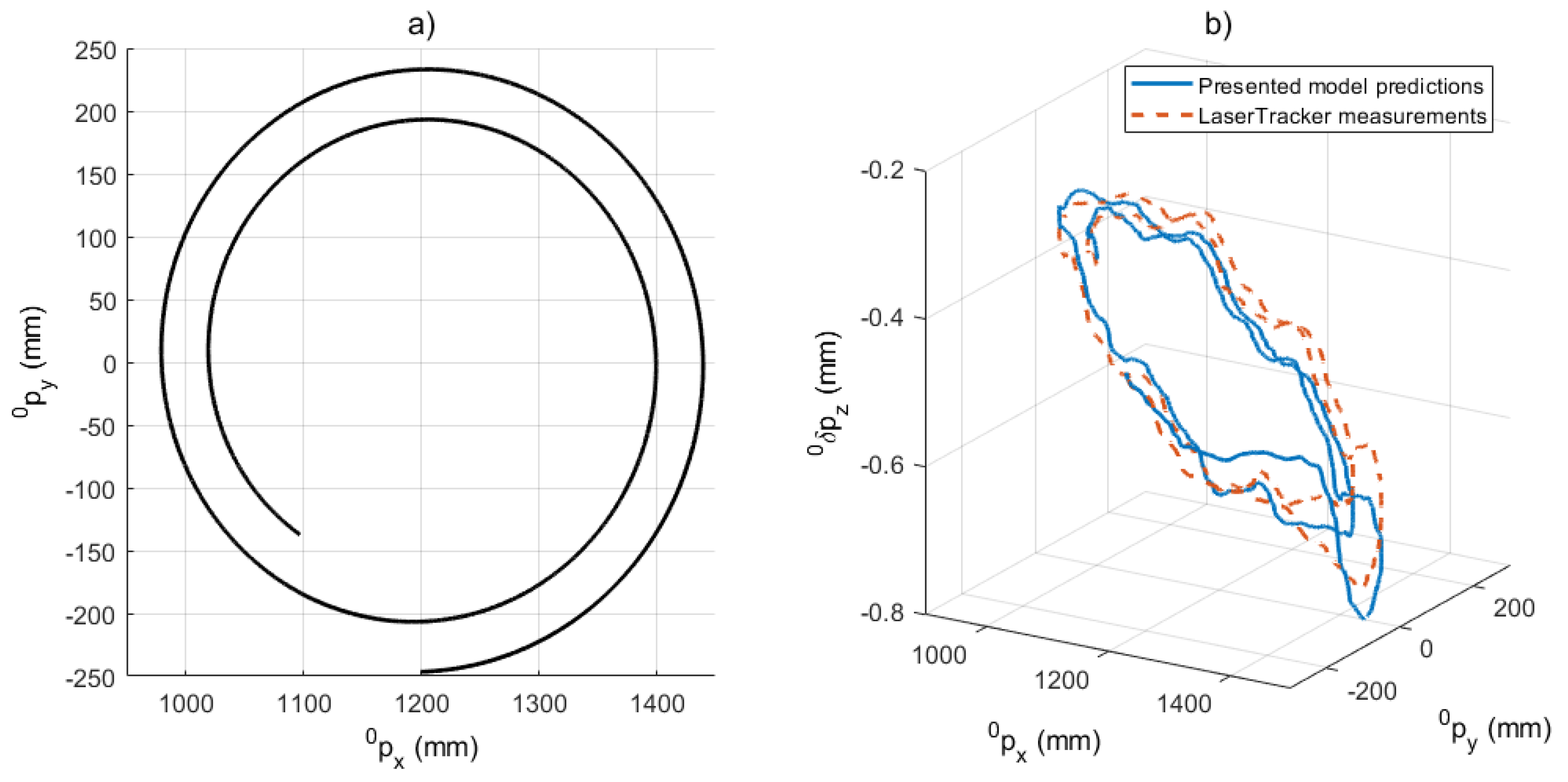
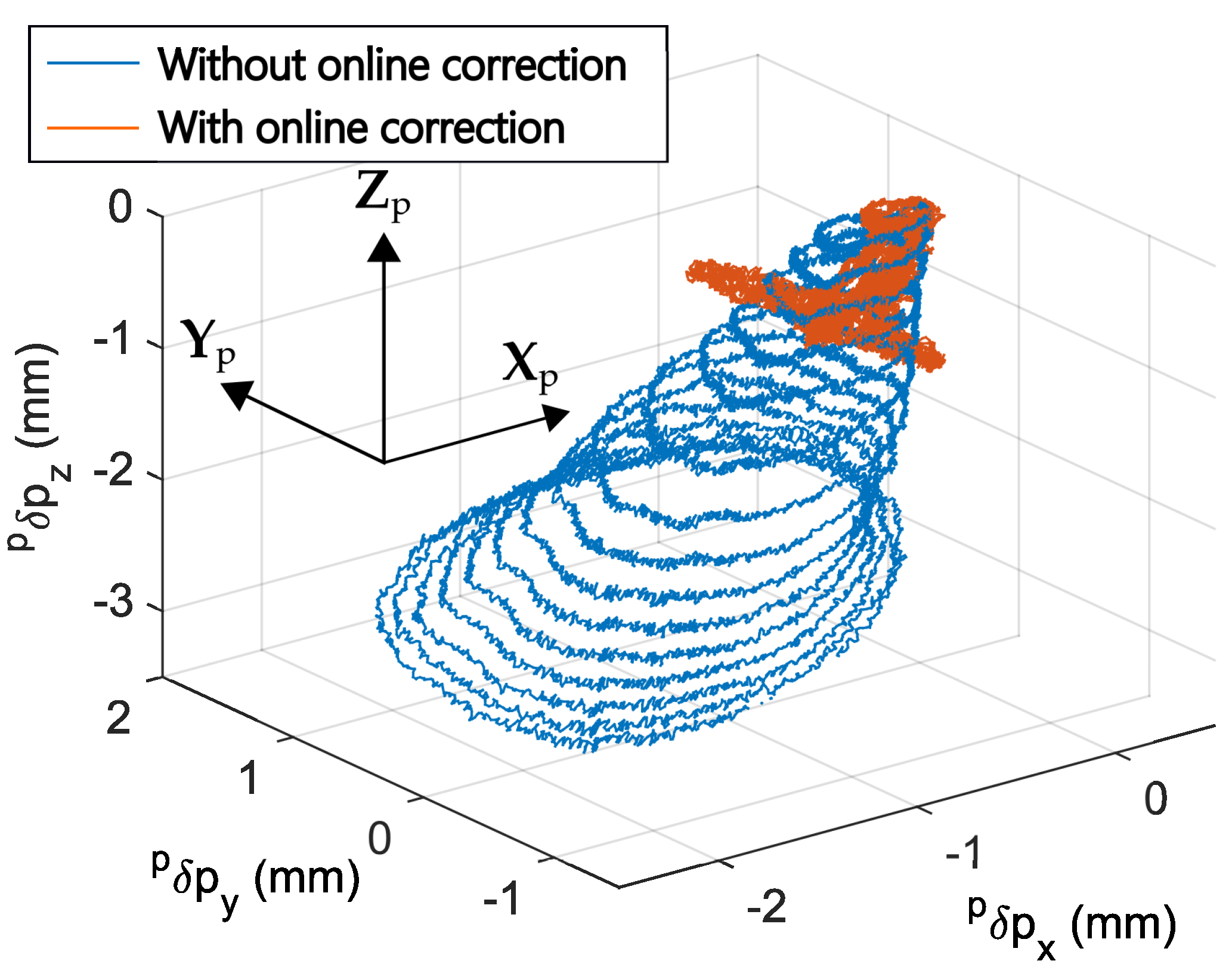
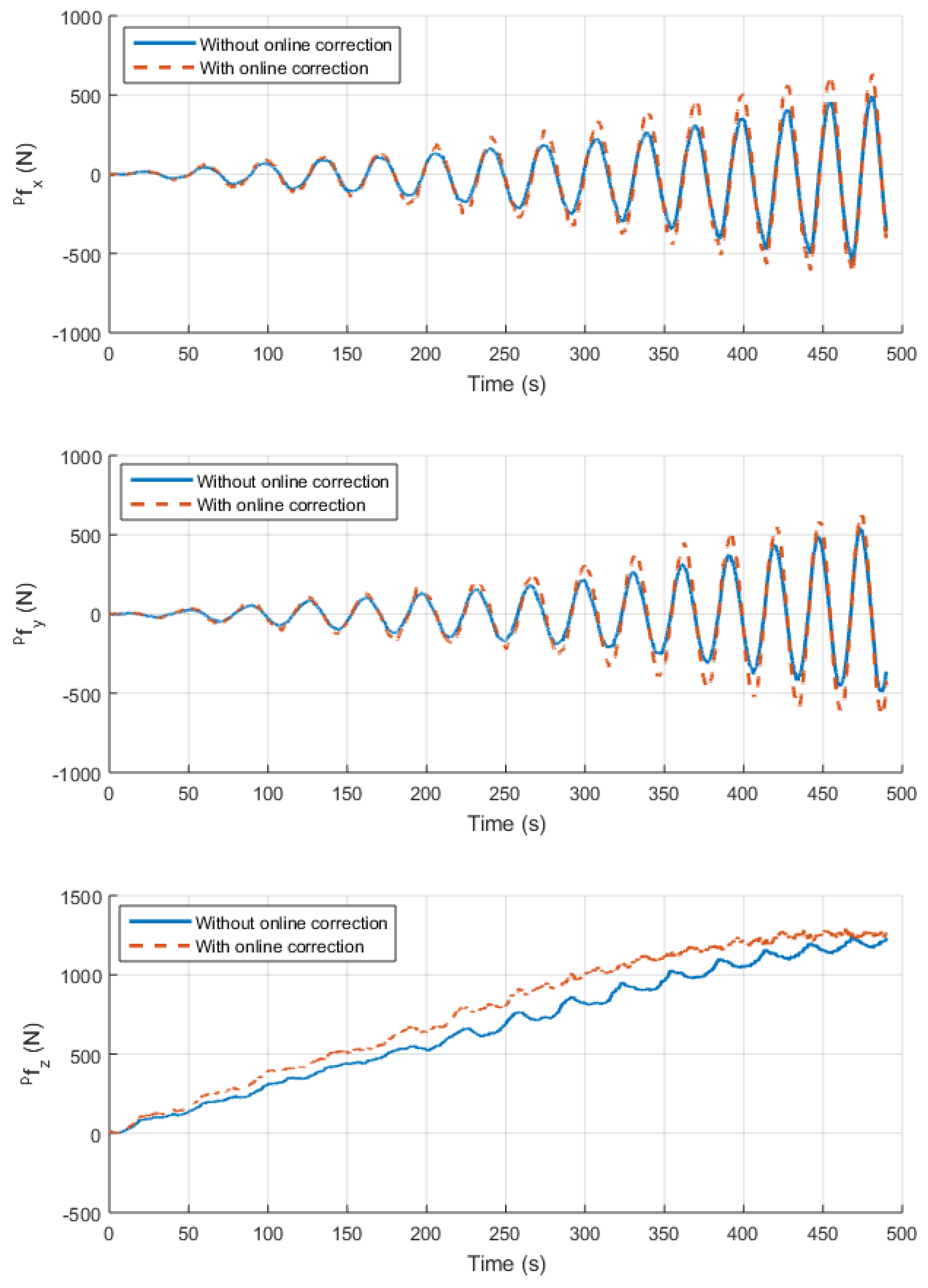
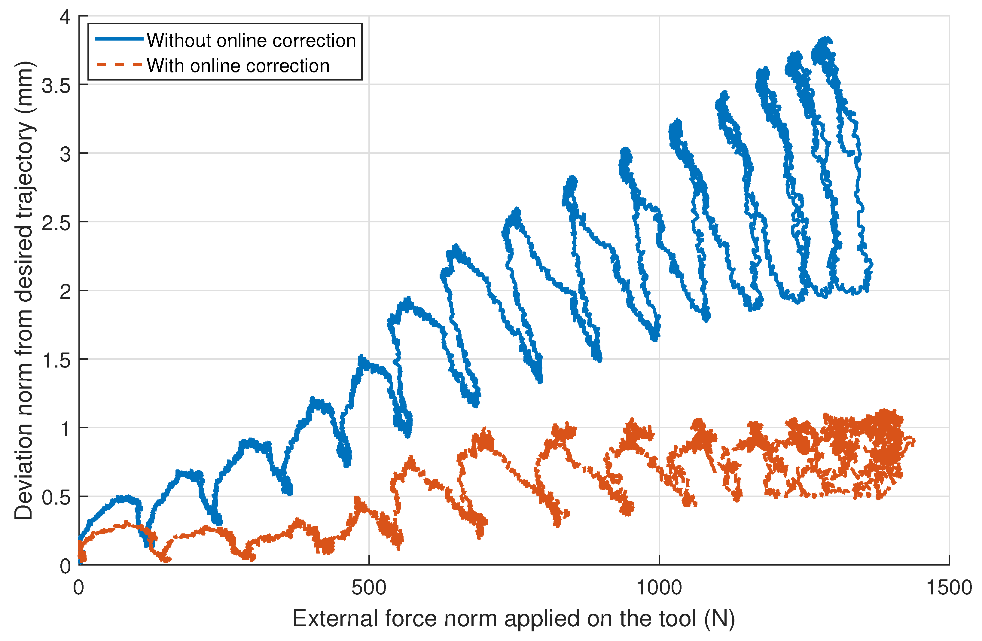
A schematic view of the real-time pose control system, developed and proposed in this study, is shown in Figure 16. As can be seen, the tool-path trajectory is computed offline from the part CAD model via a CAM software. RoboDK software was then used to convert motion planning into instructions in the Stäubli-specific robot-controller-programming language VAL 3 . The robot program was sent offline to the robot C S 8 internal controller via a TCP/IP file transfer protocol. The control algorithm was deployed in a National Instruments CompactRIO controller using the programming language LABVIEW . Two NI9215 modules collected data from the six channels of the ATI Omega-160 6-DoF load cell to determine the external wrench w acting on the forming tool. The measurement sampling frequency was set at 100 Hz.
In the LABVIEW environment, the data were processed by the external control loop (Section 2.1) to reconstruct s ^ r e a l based on the elasto-geometrical model (Equation (16)) and then compute the pose correction ξ . The resulting correction vector was sent directly to the robot internal controller through the TCP/IP protocol at a frequency of 100 Hz. This communication was compatible with the CS8 industrial robot controller, running at a fixed internal frequency of 250 Hz. Path corrections were handled online by the robot controller via the Alter function pack available in the VAL 3 language. Alter functions allowed the robot trajectory to be modified from the external controller data at the frequency of 250 Hz. During the forming process, the real tool path was measured using the API Radian laser tracker, only to validate the control strategy. An online monitoring of the process control application was then performed.
Concerning the external controller, Equation (17) was used for computing the correction vector ξ , with gains found empirically.
ξ ( t ) = K c ( ε ( t ) + 1 T i 0 t ε ( τ ) d τ + T d d ε ( t ) d t )
with K c = 0.8 , T i = 0.048 s and T d = 0.012 s .
From the FEA simulation of the process, maximum force values were used to compute the maximum correction during the trajectory. Knowing the maximum value of this correction, a verification of the system’s response was performed and the chosen PID gains allowed a response with satisfying performances. Moreover, an antiwindup algorithm and a correction limiter were added to the control loop. This way, the correction vector ξ was guaranteed to be bounded in a certain range.

4.3. Results

Figure 17 yields a readable spatial visualization of the position accuracy along the forming tool path using or not using the online correction. In the case of a perfect machine, all deviation points should be on the (0,0,0) coordinates, highlighting no elastic deformation along the three axes x p , y p , and z p . As one can see from Figure 17, a significant deviation between the desired and measured paths can be identified without online correction (blue curve). These errors are not compatible with the ISF process requirements. The robot trajectory was corrected efficiently using the online model-based control, resulting in a more centered and closer set of deviation points.
For further details, Figure A1 plots the deviation along the x p -, y p -, and z p -axes, and the norm of the deviation in position separately in the plane ( O p , x p , y p ) for the whole trajectory is noted. It is important to note that the deviation is not distributed uniformly along the path due to the resulting forces of the process (Figure 18). Obviously, this error increases in function of the TCP position along the z p -axis. In fact, the closer the tool is to the center of the frustum cone, the higher the forming forces. For this trajectory, the effort levels go up to 1200 N without online correction in the z p direction and up to 500 N along the x p - and y p -axes. For this level of force, the maximum value of the error norm is about 3.84 mm at the end of the trajectory.
A clear improvement of the global trajectory-tracking accuracy is highlighted when the online correction is applied, with a maximum value of the error norm of 1.13 mm (Figure A1). The model-based control strategy leads to a significant increase in the overall forming force to compensate for the low stiffness of the robot and brings the static equilibrium position of the TCP back to the desired trajectory (Figure 18). While applying the presented control strategy during the cone-forming experiment, the accuracy of the tool path was improved by 70 %, validating the process requirements.

5. Discussion

The forming tests prove that the presented control strategy allows an accurate position control for industrial applications such as RISF. An obvious improvement is visually highlighted in Figure 17, with the deviation from the desired trajectory corresponding to the trajectory-tracking error. Over this frustum cone trajectory, the maximum value of the trajectory-tracking error norm of 1.13 mm for a 1500 N norm load gives promising results. One feature of the results is that with the presented correction, loads above 600 N in norm rapidly worsen the accuracy, exceeding a trajectory-tracking error norm of 0.5 mm. This is even more visible when this deviation is displayed as a function of the external force norm, both measured at the robot TCP (Figure 19). It shows that after this first step, the elastic online correction keeps the deviation under a certain threshold even though a higher force norm is applied on the tool. In contrast, without online correction, the deviation keeps diverging with an increasing force norm.
The remaining error is mainly due to the structure identification and calibration of the elasto-geometrical model, keeping some room for further improvements. In the end, the validation of the presented model is successful, but some limits are visible from the number of considered eDoFs when a high wrench is applied. For example, the elastic displacement of point M 1 depicted in Figure 7 is not captured by the present model. A new iteration will probably have to thoroughly include the elastic behavior of the robot baseplate.
Obviously, this control strategy leads to an increase in the overall forming force to compensate for the elasticity of the robot, without instability of the loop or overshoot (Figure 18). The measured forces for the corrected trajectory seem to have similar ranges and trends as the ones applied by a CNC machine in the same setup [33]. It should nevertheless be kept in mind that the control method may lead to exceeding the payload capacity of the robot.
Future research should focus on increasing the operating speed to study the dynamic effects during forming, both for the control part and the elasto-geometrical modeling part. With such potential improvements, a foreseeable future for RISF is clear within tomorrow’s industry 4.0 , enabling its use for manufacturing small-batch parts, with less need for resources and energy than conventional deep drawing, while maintaining a high level of complexity and personalization of the manufactured parts.

6. Conclusions

In this paper, the absolute positioning accuracy of industrial serial manipulators was studied. A model-based control strategy was described and implemented, relying only on a force feedback for correcting the tool pose of a robotic arm (Section 2). This constraint corresponds to a real industrial cell configuration, where absolute pose tracking is often too complex or expensive to implement, whereas force control is usually a basic feature.
To compensate for the elastic deformation implied by the external wrench, an elasto-geometrical model was identified following the VJM approach. With this general approach, the full elasticity of each robotic joint is taken into account. The physical model of robots was thoroughly studied to only select the eDoFs highly influencing the tool pose accuracy. Using an efficient coupled test-model approach for identifying this model, a series of tests is needed to derive a minimum set of elastic parameters. This approach, scalable to any serial manipulator, updates the model structure after each test until a trade-off between accuracy and complexity is reached with respect to the requirements of the targeted application. This efficient identification approach was demonstrated on the Stäubli TX200 robot with a minimum number of identified stiffness parameters to ensure a good-quality prediction of the elastic deformation (Section 3).
The force-feedback model-based pose control strategy was validated through real robotic ISF tests (Section 4). The obtained results highlight a tracking accuracy improvement of 70% for the online-corrected trajectory compared to the noncorrected trajectory during a 15-mm-deep frustum cone-forming path with loads up to 1500 N in norm.
This gain in positioning accuracy improves the robot’s capabilities and allows the robotization of production processes such as ISF to manufacture parts with geometric constraints in tomorrow’s industry 4.0 .

Supplementary Materials

The following video presenting the ISF process tests performed at LGCGM is available online at https://www.mdpi.com/article/10.3390/robotics11020048/s1.

Author Contributions

Conceptualization, M.J., E.C., D.D. and S.G.; methodology, M.J., E.C., D.D.; software, M.J.; investigation, M.J., E.C., D.D., S.G.; writing—original draft preparation, M.J., D.D.; writing—review and editing, E.C., S.G.; supervision, E.C. All authors have read and agreed to the published version of the manuscript.

Funding

The authors would like to thank the European Union and the Brittany Region (FEDER funding) for their financial support allowing the purchase of specific equipment used in this work.

Data Availability Statement

The data presented in this study is contained in the article itself. Upon request to the corresponding author, Supplementary Material is available.

Conflicts of Interest

The authors declare no conflict of interest.

Abbreviations

The following symbols and acronyms are used in this manuscript:
CAMComputer-Aided Manufacturing
CADComputer-Aided Design
CNCComputer Numerical Control
FSWFriction-Stir Welding
ISFIncremental Sheet Forming
RISFRobotized Incremental Sheet Forming
VJMVirtual-Joint Method
MSAMatrix Structural Analysis
FEAFinite Element Analysis
TCPTool center Point
EEEnd-Effector
DoFDegree of Freedom
mDoFMotorized Degree of Freedom
eDoFElastic Degree of Freedom
mDHModified Denavit–Hartenberg
PIDProportional-Integral-Derivative
RMSRoot-Mean-Square

Appendix A

Table A1. Identification and calibration of the TX200 elasto-geometrical model.
Step 1 : Identification of k θ 1 , z and k θ 3 , x   q = [ 0 π 2 0 0 0 0 ] T   w = [ 0 f y 0 0 0 0 ] T
Robotics 11 00048 i001
Step 2 : Identification of k θ 2 , z   q = [ 0 0 π 2 0 0 0 ] T   w = [ f x 0 0 0 0 0 ] T
Robotics 11 00048 i002
Step 3 : Identification of k θ 3 , z q = [ 0 0 π 2 0 π 2 0 ] T   w = [ 0 0 f z 0 0 0 ] T
Robotics 11 00048 i003
Table A2. Identification and calibration of the TX200 elasto-geometrical model.
Step 4 : Identification of k θ 5 , z q = [ 0 π 2 0 0 π 2 0 ] T   w = [ f x 0 0 0 0 0 ] T
Robotics 11 00048 i004
Step 5 : Identification of k θ 4 , z   q = [ 0 0 3 π 4 0 π 2 0 ] T   w = [ 0 f y 0 0 0 0 ] T
Robotics 11 00048 i005
Figure A1. Deviation from nominal trajectory in mm along the x p -axis (a); the y p -axis (b); the z p -axis (c); and in norm (d); without online correction (left) and with online correction (right).
Robotics 11 00048 g0a1

References

  1. Roveda, L.; Piga, D. Sensorless environment stiffness and interaction force estimation for impedance control tuning in robotized interaction tasks. Auton. Robots 2021, 45, 371–388. [Google Scholar] [CrossRef]
  2. Klimchik, A.; Ambiehl, A.; Garnier, S.; Furet, B.; Pashkevich, A. Comparison Study of Industrial Robots for High-Speed Machining. In Mechatronics and Robotics Engineering for Advanced and Intelligent Manufacturing; Springer International Publishing: Cham, Switzerland, 2017; pp. 135–149. [Google Scholar] [CrossRef]
  3. Wang, X.; Wang, A.; Wang, D.; Wang, W.; Liang, B.; Qi, Y. Repetitive Control Scheme of Robotic Manipulators Based on Improved B-Spline Function. Complexity 2021, 2021, 1–15. [Google Scholar] [CrossRef]
  4. Duan, J.; Gan, Y.; Chen, M.; Dai, X. Adaptive variable impedance control for dynamic contact force tracking in uncertain environment. Robot. Auton. Syst. 2018, 102, 54–65. [Google Scholar] [CrossRef]
  5. Flacco, F.; De Luca, A.; Sardellitti, I.; Tsagarakis, N.G. On-line estimation of variable stiffness in flexible robot joints. Int. J. Robot. Res. 2012, 31, 1556–1577. [Google Scholar] [CrossRef]
  6. He, Z.; Zhang, R.; Zhang, X.; Chen, Z.; Huang, G.; Zhou, A. Absolute Positioning Error Modeling and Compensation of a 6-DOF Industrial Robot. In Proceedings of the International Conference on Robotics and Biomimetics (ROBIO), Dali, China, 6–8 December 2019; pp. 840–845. [Google Scholar] [CrossRef]
  7. dos Santos, W.M.; Siqueira, A.A. Optimal impedance via model predictive control for robot-aided rehabilitation. Control Eng. Pract. 2019, 93, 104177. [Google Scholar] [CrossRef]
  8. Santos, L.; Cortesao, R. Computed-Torque Control for Robotic-Assisted Tele-Echography Based on Perceived Stiffness Estimation. IEEE Trans. Autom. Sci. Eng. 2018, 15, 1337–1354. [Google Scholar] [CrossRef]
  9. Schempp, C.; Schulz, S. High-Precision Absolute Pose Sensing for Parallel Mechanisms. Sensors 2022, 22, 1995. [Google Scholar] [CrossRef] [PubMed]
  10. Roveda, L.; Vicentini, F.; Tosatti, L.M. Deformation-tracking impedance control in interaction with uncertain environments. In Proceedings of the 2013 IEEE/RSJ International Conference on Intelligent Robots and Systems, IEEE, Tokyo, Japan, 3–7 November 2013; pp. 1992–1997. [Google Scholar] [CrossRef]
  11. Mikhel, S.; Popov, D.; Mamedov, S.; Klimchik, A. Advancement of Robots With Double Encoders for Industrial and Collaborative Applications. In Proceedings of the IEEE Conference of Open Innovations Association (FRUCT), Bologna, Italy, 13–16 November 2018; pp. 246–252. [Google Scholar] [CrossRef]
  12. Mikhel, S.K.; Klimchik, A.S. Stiffness Model Reduction for Manipulators with Double Encoders: Algebraic Approach. Nelineinaya Dinamika 2021, 17, 347–360. [Google Scholar] [CrossRef]
  13. Dai, Y.; Xiang, C.; Qu, W.; Zhang, Q. A Review of End-Effector Research Based on Compliance Control. Machines 2022, 10, 100. [Google Scholar] [CrossRef]
  14. Guillo, M.; Dubourg, L. Impact & improvement of tool deviation in friction stir welding: Weld quality & real-time compensation on an industrial robot. Robot. Comp.-Integr. Manuf. 2016, 39, 22–31. [Google Scholar] [CrossRef]
  15. Roveda, L.; Forgione, M.; Piga, D. Robot control parameters auto-tuning in trajectory tracking applications. Control Eng. Pract. 2020, 101, 104488. [Google Scholar] [CrossRef]
  16. Karamali Ravandi, A.; Khanmirza, E.; Daneshjou, K. Hybrid force/position control of robotic arms manipulating in uncertain environments based on adaptive fuzzy sliding mode control. Appl. Soft Comput. 2018, 70, 864–874. [Google Scholar] [CrossRef]
  17. Li, B.; Tian, W.; Zhang, C.; Hua, F.; Cui, G.; Li, Y. Positioning error compensation of an industrial robot using neural networks and experimental study. Chin. J. Aeronaut. 2021, 35, 346–360. [Google Scholar] [CrossRef]
  18. Alici, G.; Shirinzadeh, B. A systematic technique to estimate positioning errors for robot accuracy improvement using laser interferometry based sensing. Mech. Mach. Theory 2005, 40, 879–906. [Google Scholar] [CrossRef]
  19. Zhang, J.; Wang, X.; Wen, K.; Zhou, Y.; Yue, Y.; Yang, J. A simple and rapid calibration methodology for industrial robot based on geometric constraint and two-step error. Ind. Robot 2018, 45, 715–721. [Google Scholar] [CrossRef]
  20. Santoni, F.; Angelis, A.D.; Skog, I.; Moschitta, A.; Carbone, P. Calibration and Characterization of a Magnetic Positioning System Using a Robotic Arm. IEEE Trans. Instrum. Meas. 2019, 68, 9. [Google Scholar] [CrossRef]
  21. Jia, Y.; Zhang, X.; Wang, Z.; Wang, W. Intelligent Calibration of a Heavy-Duty Mechanical Arm in Coal Mine. Electronics 2020, 9, 1186. [Google Scholar] [CrossRef]
  22. Shen, H.; Meng, Q.; Li, J.; Deng, J.; Wu, G. Kinematic sensitivity, parameter identification and calibration of a non-fully symmetric parallel Delta robot. Mech. Mach. Theory 2021, 161, 104311. [Google Scholar] [CrossRef]
  23. Kamali, K.; Bonev, I. Optimal Experiment Design for Elasto-Geometrical Calibration of Industrial Robots. IEEE/ASME Trans. Mechatron. 2019, 24, 2733–2744. [Google Scholar] [CrossRef]
  24. Doukas, C.; Pandremenos, J.; Stavropoulos, P.; Foteinopoulos, P.; Chryssolouris, G. On an Empirical Investigation of the Structural Behavior of Robots. Procedia CIRP 2012, 3, 501–506. [Google Scholar] [CrossRef] [Green Version]
  25. Huynh, H.N. Robotic Machining Development and Validation of a Numerical Model of Robotic Milling to Optimise the Cutting Parameters. Ph.D. Thesis, University of Mons, Mons, Belgium, 2019. [Google Scholar]
  26. Deblaise, D.; Hernot, X.; Maurine, P. A systematic analytical method for PKM stiffness matrix calculation. In Proceedings of the 2006 IEEE International Conference on Robotics and Automation, ICRA IEEE, Orlando, FL, USA, 15–19 May 2006; pp. 4213–4219. [Google Scholar] [CrossRef]
  27. Belchior, J.; Leotoing, L.; Guines, D.; Courteille, E.; Maurine, P. A Process/Machine coupling approach: Application to Robotized Incremental Sheet Forming. J. Mater. Process. Technol. 2014, 214, 1605–1616. [Google Scholar] [CrossRef] [Green Version]
  28. Pashkevich, A.; Klimchik, A.; Chablat, D. Enhanced stiffness modeling of manipulators with passive joints. Mech. Mach. Theory 2011, 46, 662–679. [Google Scholar] [CrossRef] [Green Version]
  29. Marie, S.; Courteille, E.; Maurine, P. Elasto-geometrical modeling and calibration of robot manipulators: Application to machining and forming applications. Mech. Mach. Theory 2013, 69, 13–43. [Google Scholar] [CrossRef] [Green Version]
  30. Klimchik, A.; Furet, B.; Caro, S.; Pashkevich, A. Identification of the manipulator stiffness model parameters in industrial environment. Mech. Mach. Theory 2015, 90, 1–22. [Google Scholar] [CrossRef] [Green Version]
  31. Abele, E.; Weigold, M.; Rothenbücher, S. Modeling and Identification of an Industrial Robot for Machining Applications. CIRP Annals 2007, 56, 387–390. [Google Scholar] [CrossRef]
  32. Kamali, K.; Joubair, A.; Bonev, I.A.; Bigras, P. Elasto-geometrical calibration of an industrial robot under multidirectional external loads using a laser tracker. In Proceedings of the 2016 IEEE International Conference on Robotics and Automation (ICRA), IEEE, Stockholm, Sweden, 16–21 May 2016; pp. 4320–4327. [Google Scholar] [CrossRef]
  33. Belchior, J.; Guillo, M.; Courteille, E.; Maurine, P.; Leotoing, L.; Guines, D. Off-line compensation of the tool path deviations on robotic machining: Application to incremental sheet forming. Robot. Comput.-Integr. Manuf. 2013, 29, 58–69. [Google Scholar] [CrossRef] [Green Version]
  34. Giraud-Moreau, L.; Belchior, J.; Lafon, P.; Lotoing, L.; Cherouat, A.; Courtielle, E.; Guines, D.; Maurine, P. Springback Effects During Single Point Incremental Forming: Optimization of the Tool Path. AIP Conf. Proc. 2018, 1960, 160009. [Google Scholar] [CrossRef]
  35. Chang, Z. Analytical modeling and experimental validation of the forming force in several typical incremental sheet forming processes. Int. J. Mach. Tools Manuf. 2019, 140, 62–76. [Google Scholar] [CrossRef]
  36. Kumar, S.P.; Elangovan, S.; Mohanraj, R.; Boopathi, S. Real-time applications and novel manufacturing strategies of incremental forming: An industrial perspective. Mater. Today Proc. 2021, 46, 8153–8164. [Google Scholar] [CrossRef]
  37. Coutinho, F.; Cortesão, R. Online stiffness estimation for robotic tasks with force observers. Control Eng. Pract. 2014, 24, 92–105. [Google Scholar] [CrossRef]
  38. Dumas, C.; Caro, S.; Chérif, M.; Garnier, S.; Furet, B. A methodology for joint stiffness identification of serial robots. In Proceedings of the 2010 IEEE/RSJ International Conference on Intelligent Robots and Systems, IEEE, Taipei, Taiwan, 18–22 October 2010; pp. 464–469. [Google Scholar] [CrossRef]
  39. Dumas, C.; Caro, S.; Cherif, M.; Garnier, S.; Furet, B. Joint stiffness identification of industrial serial robots. Robotica 2012, 30, 649–659. [Google Scholar] [CrossRef] [Green Version]
  40. Huynh, H.N.; Riviere-Lorphevre, E.; Verlinden, O. Multibody modelling of a flexible 6-axis robot dedicated to robotic machining. In Proceedings of the 5th Joint International Conference on Multibody System Dynamics (IMSD), Lisbon, Portugal, 24–28 June 2018. [Google Scholar]
  41. Huynh, H.N.; Assadi, H.; Dambly, V.; Rivière-Lorphèvre, E.; Verlinden, O. Direct method for updating flexible multibody systems applied to a milling robot. Robot. Comput.-Integr. Manuf. 2021, 68, 102049. [Google Scholar] [CrossRef]
  42. Alici, G.; Shirinzadeh, B. Enhanced stiffness modeling, identification and characterization for robot manipulators. IEEE Trans. Robot. 2005, 21, 554–564. [Google Scholar] [CrossRef] [Green Version]
  43. Dumas, C.; Caro, S.; Garnier, S.; Furet, B. Joint stiffness identification of six-revolute industrial serial robots. Robot. Comput.-Integr. Manuf. 2011, 27, 881–888. [Google Scholar] [CrossRef] [Green Version]
  44. Martins, P.; Bay, N.; Skjoedt, M.; Silva, M. Theory of single point incremental forming. CIRP Annals 2008, 57, 247–252. [Google Scholar] [CrossRef]
  45. Behera, A.K.; de Sousa, R.A.; Ingarao, G.; Oleksik, V. Single point incremental forming: An assessment of the progress and technology trends from 2005 to 2015. J. Manuf. Process. 2017, 27, 37–62. [Google Scholar] [CrossRef] [Green Version]
  46. Duflou, J.R.; Habraken, A.M.; Cao, J.; Malhotra, R.; Bambach, M.; Adams, D.; Vanhove, H.; Mohammadi, A.; Jeswiet, J. Single point incremental forming: State-of-the-art and prospects. Int. J. Mater. Form. 2018, 11, 743–773. [Google Scholar] [CrossRef]
Figure 1. Block diagram of the force-feedback elasto-geometrical model-based control.
Robotics 11 00048 g001
Figure 2. Definition of the TCP and its attached frame R t .
Robotics 11 00048 g002
Figure 3. Deflection of the TCP due to the external wrench w applied on the tool: desired (a); real (b); configurations.
Robotics 11 00048 g003
Figure 4. Elastic joint architecture using the VJM approach.
Robotics 11 00048 g004
Figure 5. Virtual Joint Method stiffness model of the i t h joint.
Robotics 11 00048 g005
Figure 6. Flow chart of the coupled test-model approach used for identifying the elasto-geometrical model.
Robotics 11 00048 g006
Figure 7. Specific configuration for stiffness model structure identification and calibration of the Stäubli TX200 (top view): articular configuration q = [ 0 π 2 0 0 0 0 ] T ; external wrench w = [ 0 f y 0 0 0 0 ] T with the maximum value being f y = 1400 N.
Robotics 11 00048 g007
Figure 8. Elastic displacement δ p x measured for several points along the x 0 -axis and estimated by the one-eDoF-per-joint model and the presented model: articular configuration q = [ 0 π 2 0 0 0 0 ] T ; external wrench w = [ 0 f y 0 0 0 0 ] T with f y = 1400 N.
Robotics 11 00048 g008
Figure 9. Elastic displacement δ p y measured for several points along the x 0 -axis and estimated by the one-eDoF-per-joint model and the presented model: articular configuration q = [ 0 π 2 0 0 0 0 ] T ; external wrench w = [ 0 f y 0 0 0 0 ] T with f y = 1400 N.
Robotics 11 00048 g009
Figure 10. Comparison of 0 δ p z error for the presented model predictions (blue), one-eDoF-per-joint elastic model predictions (red) and experimental measurements (green) in a 0.6-by-0.6 meter square workspace plane with a vertical applied force of 600 N.
Robotics 11 00048 g010
Figure 11. Heatmaps of the deviation between the one-eDoF-per-joint model predictions and experimental measurements (a); and between the presented model predictions and experimental measurements (b); both for a vertical applied force of 600 N.
Robotics 11 00048 g011
Figure 12. Comparison of 0 δ p z error for the presented model predictions (blue), one-eDoF-per-joint elastic model predictions (red) and experimental measurements (green) in a 0.6-by-0.6 meter square workspace plane with a vertical applied force of 1100 N.
Robotics 11 00048 g012
Figure 13. Heatmaps of the deviation between the one-eDoF-per-joint model predictions and experimental measurements (a); and between the presented model predictions and experimental measurements (b); both for a vertical applied force of 1100 N.
Robotics 11 00048 g013
Figure 14. (a) Desired spiral trajectory; (b) Comparison of 0 δ p z error for the presented model predictions (continuous blue) and experimental measurements (dashed orange) along a spiral trajectory with a constant vertical load of 600 N.
Robotics 11 00048 g014
Figure 15. Position of the ISF setup inside the robotic cell (left); desired tool path and CAD model of the clamping system with a formed metal sheet (right).
Robotics 11 00048 g015
Figure 16. Schematic view of the real-time model-based force-feedback pose control.
Robotics 11 00048 g016
Figure 17. Deviation from desired trajectory measured at the TCP during the cone-forming experiment without and with online correction.
Robotics 11 00048 g017
Figure 18. External force along the x p -, y p - and z p -axes measured at the robot TCP during the cone-forming experiment without and with online correction.
Robotics 11 00048 g018
Figure 19. Trajectory-tracking error norm as a function of the external force norm (both measured at the robot TCP during the cone forming experiment without and with online correction).
Robotics 11 00048 g019
Table 1. Torsional stiffness parameters k θ i , j of the Stäubli TX200 ( 10 6   Nm · rad 1 ).
Joint 1Joint 2Joint 3Joint 4Joint 5Joint 6
k θ i , x --1.45---
k θ i , y ------
k θ i , z 2.321.762.040.090.02-
Publisher’s Note: MDPI stays neutral with regard to jurisdictional claims in published maps and institutional affiliations.

